Delay Analysis of Random Scheduling and Round Robin in Small Cell Networks

Abstract

We analyze the delay performance of small cell networks operating under random scheduling (RS) and round robin (RR) protocols. Based on stochastic geometry and queuing theory, we derive accurate and tractable expressions for the distribution of mean delay, which accounts for the impact of random traffic arrivals, queuing interactions, and failed packet retransmissions. Our analysis asserts that RR outperforms RS in terms of mean delay, regardless of traffic statistic. Moreover, the gain from RR is more pronounced in the presence of heavy traffic, which confirms the importance of accounting fairness in the design of scheduling policy. We also find that constrained on the same delay outage probability, RR is able to support more user equipments (UEs) than that of RS, demonstrating it as an appropriate candidate for the traffic scheduling policy of internet-of-things (IoT) network.

I Introduction

The paradigm shift from traditional macro cellular network to small cell networks is unrelenting, whereas more and more user equipments (UEs), including smartphones, tablets, and smartwatches, will be connected to the small access points (SAPs) [1]. Since the wireless spectrum is usually limited, there is inevitable contention among UEs for communication resource. At this stage, operators need to choose an appropriate traffic scheduling protocol to allocate resource among different UEs so as to meet the delay requirement [1]. Among the large number of proposed scheduling schemes [2], random scheduling (RS) and round robin (RR) are the most popular practical choices due to their low-implementation cost [3]. Even though, a full understanding on the respective delay performance of RS and RR is still essential to help devise insights and perform suitable design. While the delay performance of both schemes has been well understood in wired data networks [3], it remains in darkness from the perspective of wireless small cell networks because: $i$) the irregular deployment of SAPs leads to asymmetric UE performance, e.g., some UEs may succeed in capturing a large portion of resources than others because of their relative position in the network, and thus enjoy preferential treatment; $ii$) the shared nature of wireless channel results in the queuing evolution of any typical cell strongly interacted with its neighbors, which piles on analytical complications.

Most of the previous works only focus on one aspect of the issue [3, 4, 5, 6], i.e., they model only the temporal arrival of packets [3] or the spatial lotations [4, 5, 6], and thus fail to track the other. Recently, several attempts have been made to analyze delay in large-scale networks by modeling the spatial-temporal randomness [7, 8, 9, 10]. However, the results in [7] only give upper and lower bounds, that can be loose in light traffic condition, for the delay distribution, hence may fail to explicitly capture the interplay between spatial topology and temporal queuing evolution. While [8] attains a precise expression for the distribution of mean delay, the result holds for single UE per cell scenario, which do not allow one to investigate the effect of different scheduling policies. The model in [9, 10] consider uplink random access for multi-UE per cell and accounts for the intra-cell and inter-cell interference due to the scheduling policy. However, the results only analyze the RS and do not extend to other scheduling methods.

In this work, we take a complete treatment to the delay analysis in small cell networks under different traffic scheduling policies. Specifically, we model the locations of SAPs as homogeneous Poisson point process (PPP) where each cell has multiple associated UEs. The traffic arrivals are modeled as independent Bernoulli processes, and account for the retransmission of unsuccessfully delivered packets. By combining stochastic geometry with queueing theory, we derive accurate expressions for the mean delay distribution under both RS and RR protocols, allowing to compare them and to draw insightful conclusions.

II System Model

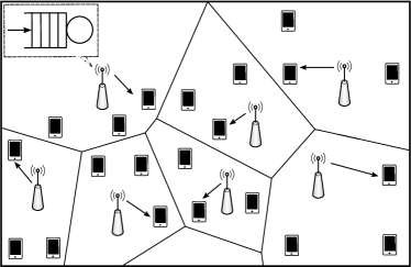
Figure 1: Example of a small cell network with random traffic arrivals.

We consider the downlink of a small cell network, as depicted in Fig. 1, that consists of randomly deployed SAPs. We model the spatial locations of SAPs as a homogeneous PPP $\Phi_{\mathrm{s}}$ with spatial density $\lambda_{\mathrm{s}}$. For notational simplicity, we assume each SAP has $K_{\mathrm{s}}$ associated UEs, who are uniformly distributed within the Voronoi cell it generated. All SAPs and UEs are equipped with single antenna, and every SAP transmits with power $P_{\mathrm{st}}$. We assume the channels between any pair of nodes to be narrowband and affected by two attenuation components, namely small-scale Rayleigh fading, and large-scale path loss.

We use a discrete time queuing system to model the traffic profile, and segment the time axis into slots with equal duration. We assume all queuing activities, i.e., packet arrivals and departures, take place at each time slot. For a generic UE, we model its packet arrivals as independent Bernoulli processes with rates $\xi\in[0,1]$ (packet/slot) [7, 9, 8]. We further assume that each node accumulates all incoming packets in an infinite-size buffer. At the beginning of any typical time slot, every node with a non-empty buffer initiates a transmission attempt. If the received signal-to-interference ratio (SIR) exceeds a predefined threshold, the transmission is successful and the packet can be removed from the queue, otherwise, the transmission fails and the packet remains in the buffer. We assume the feedback of each transmission, either success or fail, can be instantaneously aware by the SAPs such that they are able to schedule transmission at next time slot. Moreover, for those SAPs with empty buffers, they mute the transmissions to reduce power consumption and inter-cell interference.

In the following, we investigate two traffic scheduling protocols, i.e., random scheduling (RS) and round robin (RR), described as below [7].

II-1 Random Scheduling

During each time slot, every active SAP randomly selects one of its UEs to serve.

II-2 Round Robin

The SAPs arrange their UEs in a sequential order, and successively select one of the UEs to serve in each slot.

$$F^{\Phi}(u)=\frac{1}{2}-\frac{1}{\pi}\int_{0}^{\infty}\frac{1}{\omega}\mathrm{Im}\left\{u^{-j\omega}\left[1+\delta\sum_{k=1}^{\infty}\binom{j\omega}{k}\left(F^{\Phi}(\xi K_{\mathrm{s}})+\int_{\xi K_{\mathrm{s}}}^{1}\frac{\left(\xi K_{\mathrm{s}}\right)^{k}}{t^{k}}F^{\Phi}(dt)\right)\mathcal{Z}(k,\delta,\theta)\right]^{-1}\right\}d\omega$$ (6)

 

III Analysis

III-A Preliminaries

III-A1 Service Rate

Using the Slivnyak’s theorem [12], we can focus on a typical UE who locates at the origin and receives data from its tagged SAP at $x_{0}$. The corresponding service rate at time slot $t$ can then be written as

$$\mu_{x_{0},t}^{\Phi}=\mathbb{P}\left(\frac{P_{\mathrm{st}}h_{x_{0}}\|x_{0}\|^{-\alpha}}{\sum\limits_{x\in\Phi_{\mathrm{s}}\setminus x_{0}}{P_{\mathrm{st}}\zeta_{x,t}h_{x}}{\|x\|^{-\alpha}}}>\theta\Bigg{|}\Phi_{\mathrm{s}}\right),$$ (1)

where $h_{x}$ is the channel fading from SAP $x$ to the origin, $\alpha$ is the path loss exponent, $\theta$ the SIR decoding threshold, and $\zeta_{x,t}\in\{0,1\}$ represents an indicator showing whether an SAP located at $x\in\Phi_{\mathrm{s}}$ is transmitting at time slot $t$ (in this case, $\zeta_{x,t}=1$) or not (in this case, $\zeta_{x,t}=0$).

Due to the broadcast nature of wireless medium, the queuing status of each SAP is coupled with other transmitters and hence results in interacting queue [13]. Consequently, the SAP active state, $\zeta_{x,t}$, is both spatial and temporal dependent: The spatial locations determine how the SAPs interfere with each other, and the temporal traffic dynamic affects the queue evolution. Moreover, as a generic UE may see common interferencing SAPs in consecutive time slots, the system service rate is temporally correlated [14, 9, 15]. Such temporal correlation introduces memory to the queue and can highly complicate the analysis. In the following, we assume each link experiences independent service rate across time to maintain the mathematical tractability [9, 15].

III-A2 Mean Delay

In this paper, we adopt the mean delay, i.e., the average number of required slots for one successful packet transmission, as our performance metric. A formal definition is given as follows.

Definition 1

Let $A_{x}(T)$ be the number of packets arrived at a typical transmitter $x$ within period $[0,T]$, and $D_{i,x}$ be the number of time slots between the arrival of the $i$-th packet and its successful delivery. The mean delay is defined as

$$\mathbf{D}_{x}\triangleq\lim\limits_{T\rightarrow\infty}\frac{\sum_{i=1}^{A_{x}(T)}D_{i,x}}{A_{x}(T)}.$$ (2)

Note that $\mathbf{D}_{x}$ encapsulates the cross-network delay information as it is obtained by sampling at a random transmitter. Moreover, while $\mathbf{D}_{x}$ is defined via ergodic average, it is nevertheless a random variable because of the random service rate. Besides, the element $D_{i,x}$ in (2) refers to the total amount of time that the $i$-th packet is in the queuing system, both in the queue (caused by other accumulated unsent packets) and in the service (due to link failure and retransmission).

III-B Delay Analysis

This section details the main results of our work. First of all, we condition on the random service rate, and give an explicit form of the mean delay for RS protocol.

Lemma 1

Given the UE number $K_{\mathrm{s}}$, the arrival rate $\xi$, and the service rate $\mu^{\Phi}_{x_{0}}$, the mean delay at a typical SAP under RS is given by

$$\mathbf{D}_{x_{0}}^{\mathrm{RS}}=\left\{\!\!\!\begin{tabular}[]{cc}$\frac{1-\xi}{\frac{\mu^{\Phi}_{x_{0}}}{K_{\mathrm{s}}}-\xi}$,&if $\mu^{\Phi}_{x_{0}}/K_{\mathrm{s}}>\xi$,\\ +$\infty$,&if $\mu^{\Phi}_{x_{0}}/K_{\mathrm{s}}\leq\xi$.\end{tabular}\right.$$ (5)

and the queue non-empty probability is given by

$$\tau_{a}^{\mathrm{RS}}=\min\{{K_{\mathrm{s}}\xi}/{\mu^{\Phi}_{x_{0}}},1\}.$$ (6)

Proof:

See [7, 11] for a detail proof. ∎

The distribution of mean delay under RS protocol can be readily derived.

Theorem 1

The cumulative distribution function (CDF) of the mean delay under RS is given by

$$\mathbb{P}\left(\mathbf{D}_{x_{0}}^{\mathrm{RS}}\leq T\right) ={1-F^{\Phi}\left(\left(\frac{1-\xi}{T}+\xi\right)K_{\mathrm{s}}\right)}$$ (7)

where $F^{\Phi}(x)$ is given by the fixed-point equation (6) on top of this page, with $\delta=2/\alpha$, $\mathrm{Im}\{\cdot\}$ being the imaginary part of a complex number, and $\mathcal{Z}(k,\delta,\theta)$ written as

$$\mathcal{Z}(k,\delta,\theta)=\frac{(-1)^{k+1}\theta^{k}}{k-\delta}{}_{2}F_{1}(k,k-\delta;k-\delta+1,-\theta),$$ (7)

whereas ${}_{2}F_{1}(a,b;c,d)$ is the hypergeometry function [8].

Proof:

See [8] for a detail proof. ∎

The function given in (6) can be solved via an iterative approach, and low-computational-complexity approximation is available to boost up the convergent speed [8].

In regard to the RR protocol, we notice that each UE is scheduled to access the wireless channel in deterministic pattern. Hence, by conditioning on the service rate, we obtain an explicit form of mean delay as below.

Lemma 2

Given the UE number $K_{\mathrm{s}}$, the arrival rate $\xi$, and the service rate $\mu^{\Phi}_{x_{0}}$, the mean delay at a typical SAP under RR is given as

$$\mathbf{D}_{x_{0}}^{\mathrm{RR}}=\left\{\!\!\!\!\!\!\!\!\!\!\begin{tabular}[]{cc}&$\frac{1-{(K_{\mathrm{s}}+1)\xi}/{2}}{{\mu^{\Phi}_{x_{0}}}/{K_{\mathrm{s}}}-\xi}$ - $\frac{K_{\mathrm{s}}-1}{2}$, if $\mu^{\Phi}_{x_{0}}/K_{\mathrm{s}}>\xi$,\\ &+$\infty$, $\qquad\qquad\qquad$ if $\mu^{\Phi}_{x_{0}}/K_{\mathrm{s}}\leq\xi$.\end{tabular}\right.$$ (10)

and the queue non-empty probability is given by

$$\tau_{a}^{\mathrm{RR}}=\min\{{K_{\mathrm{s}}\xi}/{\mu^{\Phi}_{x_{0}}},1\}.$$ (11)

Proof:

See Appendix -A for a sketch of the proof. ∎

With the above result, the distribution of mean delay under RR can be derived subsequently.

Theorem 2

The CDF of the mean delay under RR is given by

$$\mathbb{P}\left(\mathbf{D}_{x_{0}}^{\mathrm{RR}}\leq T\right) ={1-F^{\Phi}\left(\left(\frac{1-\frac{(K_{\mathrm{s}}+1)}{2}\xi}{T+\frac{K_{\mathrm{s}}-1}{2}}+\xi\right)K_{\mathrm{s}}\right)}$$ (12)

where $F^{\Phi}(x)$ is given by (6).

Proof:

The proof is similar to that of Theorem 1. ∎

Remark 1

From Lemma 1 and Lemma 2, we note that when $\mu^{\Phi}_{x_{0}}/K_{\mathrm{s}}>\xi$, there is $\mathbf{D}_{x_{0}}^{\mathrm{RS}}-\mathbf{D}_{x_{0}}^{\mathrm{RR}}\!=\!\frac{K_{\mathrm{s}}-1}{2}\frac{\mu^{\Phi}_{x_{0}}}{\mu^{\Phi}_{x_{0}}-K_{\mathrm{s}}\xi}>0$. This observation confirms that RR outperforms RS in terms of delay regardless of traffic condition, which is in line with [7].

Remark 2

Take $T=1$ in the expressions of Theorem 1 and Theorem 2, we find that $\mathbb{P}\left(\mathbf{D}_{x_{0}}^{\mathrm{RS}}\leq 1\right)=\mathbb{P}\left(\mathbf{D}_{x_{0}}^{\mathrm{RR}}\leq 1\right)=0$, i.e., the UEs that are able to success without retransmission form a probabilistic null set in small cell networks.

Remark 3

When $T\gg 1$, we have $\mathbb{P}\left(\mathbf{D}_{x_{0}}^{\mathrm{RS}}>T\right)\approx F^{\Phi}(\xi K_{\mathrm{s}})+1/T$ and $\mathbb{P}\left(\mathbf{D}_{x_{0}}^{\mathrm{RR}}>T\right)\approx F^{\Phi}(\xi K_{\mathrm{s}})+1/T$, which reveals that the CDF of mean delay obeys fat tail property.

IV Simulation and Numerical Results

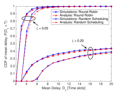
Figure 2: CDF of mean delay: Simulations vs Analysis.

We now give simulation results that validate the accuracy of our analysis, and numerical results to compare the performance of the employed scheduling schemes. Unless otherwise stated, we adopt the following system parameters [11, 7]: $\lambda_{\mathrm{s}}=10^{-4}\mathrm{m}^{-2}$, $P_{\mathrm{st}}=23$ dBm, $K_{\mathrm{s}}=3$, $\theta=0$ dB, $T_{0}=20$, and $\alpha=3.8$.

In Fig. 2, we plot the CDF of mean delay under two different traffic statistics, namely, light traffic (where $\xi=0.05$) and heavy traffic (where $\xi=0.20$). The figure shows a close match between simulations and analytical results, thus validates Theorem 1 and Theorem 2. Moreover, it can be seen that RR attains smaller mean delay than RS in both light and heavy traffic regime, which is consistent with Remark 1. Additionally, we note that the gain from RR is more pronounced under heavy traffic condition. Because when traffic profile grows, not only more newly arrived packets will build up the buffer, that incurs longer queuing delay, but more severely, more idle SAPs are activated and hence increases the interference, which results in longer transmission delay. Under such circumstance, a scheduling protocol that regulates network inputs and grants each UE a fair service opportunity is critical for delay performance. Hence, compared to RS that provides only random channel access, RR is able to achieve much better gain in delay via regulated access control.

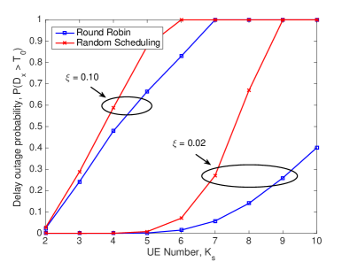
Figure 3: Delay outage probability versus per-cell UE number.

Fig. 3 depicts the delay outage probability, i.e., $\mathbb{P}(\mathbf{D}_{x}>T_{0})$, as a function of UE number, $K_{\mathrm{s}}$, per cell. This figure gives information about the scablility, which is crucial for internet-of-things (IoT) applications [9], of both scheduling protocols. We can see that while RR possesses a better scability than RS, the relative performance varies with the traffic conditions, namely: $i$) in the presence of light traffic, i.e., $\xi=0.02$, RR can support much more UEs with relatively small delay outage probability than that of RS; $ii$) in the medium to heavy traffic regime, i.e., $\xi=0.10$, the delay outage probabilities under the two scheduling policies tends to be more alike as UE number grows.

V Conclusion

In this paper, we conducted a study on the delay performance of small cell networks under random scheduling (RS) and round robin (RR) protocols. For networks where both topology and traffic arrivals are random, we analyzed the mean delay by accounting for effects from queuing, retransmissions, and spatial-temporal interactions. Our results confirmed that RR outperforms RS regardless of traffic condition, and the gain from RR is especially significant in the presence of heavy traffic, which demonstrates the importance of accounting fairness in the design of scheduling policy. Moreover, we found that by using RR, the network can support larger amount of UEs with relatively small delay outage probability than that of RS, hence appeals RR as a suitable candidate for scheduling protocols in IoT applications.

-A Sketch of Proof of Lemma 2

Under round robin, a typical UE is scheduled for transmission in every $K_{\mathrm{s}}$ slots. During the time slots when the UE is not scheduled, there is only packet arrivals, and the queue state transitioin matrix is given by

$$\mathbf{P}_{\mathrm{A}}\!=\!\begin{bmatrix}~{}1-\xi&\!\!\!\!\!\xi&\!\!0&\!\!\!\cdots&\!\!\!\!\!\cdots&\!\!\!\!\!\cdots&\!\!\!0&\!\!\!0&\!\!\!\cdots\ \\ ~{}0&\!\!\!\!\!1-\xi&\!\!\!\xi&\!\!\!0&\!\!\!\!\!\cdots&\!\!\!\!\!\cdots&\!\!\!0&\!\!\!0&\!\!\!\cdots\ \\ ~{}\vdots&\!\!\!\!\!\vdots&\!\!\!\vdots&\!\!\!\vdots&\!\!\!\!\!\ddots&\!\!\!\!\!\cdots&\!\!\!0&\!\!\!0&\!\!\!\cdots\ \\ ~{}0&\!\!\!\!\!0&\!\!\!0&\!\!\!0&\!\!\!\!\!\cdots&\!\!\!\!\!1-\xi&\!\!\!\xi&\!\!\!0&\!\!\!\cdots\ \\ ~{}\vdots&\!\!\!\!\!\vdots&\!\!\!\vdots&\!\!\!\vdots&\!\!\!\!\!\vdots&\!\!\!\!\!\vdots&\!\!\!\vdots&\!\!\!\vdots&\!\!\!\ddots\ \end{bmatrix}.$$

During the scheduled transmission slots, the queue state transition matrix can be written as follows

$$\mathbf{P}_{\mathrm{D}}\!=\!\begin{bmatrix}~{}1-\xi&\!\!\!\!\!\xi&\!\!\!\!\!0&\!\!\!\!\!\cdots&\!\!\!\!\!\cdots&\!\!\!\!\!\cdots&\!\!\!\!\!0&\!\!\!\!\!0&\!\!\!\!\!\cdots\ \\ ~{}\kappa_{2}&\!\!\!\!\!\kappa_{3}&\!\!\!\!\!\kappa_{1}&\!\!\!\!\!0&\!\!\!\!\!\cdots&\!\!\!\!\!\cdots&\!\!\!\!\!0&\!\!\!\!\!0&\!\!\!\!\!\cdots\ \\ ~{}0&\!\!\!\!\!\kappa_{2}&\!\!\!\!\!\kappa_{3}&\!\!\!\!\!\kappa_{1}&\!\!\!\!\!0&\!\!\!\!\!\cdots&\!\!\!\!\!0&\!\!\!\!\!0&\!\!\!\!\!\cdots\ \\ ~{}\vdots&\!\!\!\!\!\vdots&\!\!\!\!\!\vdots&\!\!\!\!\!\vdots&\!\!\!\!\!\ddots&\!\!\!\!\!\cdots&\!\!\!\!\!0&\!\!\!\!\!0&\!\!\!\!\!\cdots\ \\ ~{}0&\!\!\!\!\!0&\!\!\!\!\!0&\!\!\!\!\!0&\!\!\!\!\!\cdots&\!\!\!\!\!\kappa_{2}&\!\!\!\!\!\kappa_{3}&\!\!\!\!\!\kappa_{1}&\!\!\!\!\!\cdots\ \\ ~{}\vdots&\!\!\!\!\!\vdots&\!\!\!\!\!\vdots&\!\!\!\!\!\vdots&\!\!\!\!\!\vdots&\!\!\!\!\!\vdots&\!\!\!\!\!\vdots&\!\!\!\!\!\vdots&\!\!\!\!\!\ddots\ \end{bmatrix}$$

where $\kappa_{1}$, $\kappa_{2}$, and $\kappa_{3}$ are respectively given by

$$\kappa_{1} =\xi(1-\mu^{\Phi}_{x_{0}}),\quad\kappa_{2}=(1-\xi)\mu^{\Phi}_{x_{0}},$$ (13)

$$\kappa_{3} =(1-\xi)(1-\mu^{\Phi}_{x_{0}})+\xi\mu^{\Phi}_{x_{0}}.$$ (14)

Without loss of generality, we let the timing start from the moment the UE just been scheduled, hence, the queue transition matrix in a complete transmission round can be written as

$$\mathbf{P}_{\mathrm{T}}=\underbrace{\mathbf{P}_{\mathrm{A}}\times\mathbf{P}_{\mathrm{A}}\times\cdots\times\mathbf{P}_{\mathrm{A}}}_{K_{\mathrm{s}}-1}\times\mathbf{P}_{\mathrm{D}}$$ (15)

where the product is performed with respect to the regular matrix multiplication. Let $\mathbf{v}=\left(v_{1},v_{2},...\right)$ denote the steady state probability vector, then, in the steady state, we have

$${}\mathbf{v}\mathbf{P}_{\mathrm{T}} =\mathbf{v},$$ (16)

$$\sum_{i=0}^{\infty}v_{i} =1.$$ (17)

Solving the above system equation yields the individual elements $\{v_{i}\}_{i=0}^{\infty}$, the queue non-empty probability corresponds to $\tau^{\mathrm{RR}}_{x_{0}}=1-v_{0}$, and the mean delay can then be obtained as

$$\mathbf{D}_{x_{0}}^{\mathrm{RR}}=\sum_{i=0}^{\infty}iv_{i}+\frac{1}{\mu^{\Phi}_{x_{0}}}.$$ (18)

References

- [1] J. G. Andrews, S. Buzzi, W. Choi, S. V. Hanly, A. Lozano, A. C. K. Soong, and J. C. Zhang, “What will 5G be?” IEEE J. Sel. Areas Commun., vol. 32, no. 6, pp. 1065–1082, Jun. 2014.
- [2] M. Gerla and L. Kleinrock, “Flow control: A comparative survey,” IEEE Trans. Commun., vol. 28, no. 4, pp. 553–574, Apr. 1980.
- [3] E. L. Hahne, “Round-robin scheduling for max-min fairness in data networks,” IEEE J. Sel. Areas Commun., vol. 9, no. 7, pp. 1024–1039, Sep. 1991.
- [4] G. Zhang, T. Q. S. Quek, A. Huang, and H. Shan, “Delay and reliability tradeoffs in heterogeneous cellular networks,” IEEE Trans. Wireless Commun., vol. 15, no. 2, pp. 1101–1113, Feb. 2016.
- [5] M. Ding, D. L. Pérez, A. H. Jafari, G. Mao, and Z. Lin, “Ultra-dense networks: A new look at the proportional fair scheduler,” Available as arXiv: 1708.07961, 2017.
- [6] A. H. Jafari, D. López-Pérez, M. Ding, and J. Zhang, “Study on scheduling techniques for ultra dense small cell networks,” in Proc. of Vehicular Technology Conference (VTC Fall), Boston, MA, Sept. 2015, pp. 1–6.
- [7] Y. Zhong, T. Q. S. Quek, and X. Ge, “Heterogeneous cellular networks with spatio-temporal traffic: Delay analysis and scheduling,” IEEE J. Sel. Areas Commun., vol. 35, no. 6, pp. 1373–1386, Jun. 2017.
- [8] H. H. Yang and T. Q. S. Quek, “SIR coverage analysis in cellular networks with temporal traffic: A stochastic geometry approach,” Available as arXiv:1612.01276, 2018.
- [9] M. Gharbieh, H. ElSawy, A. Bader, and M.-S. Alouini, “Spatiotemporal stochastic modeling of IoT enabled cellular networks: Scalability and stability analysis,” IEEE Trans. Commun., vol. 65, no. 9, pp. 3585–3600, Aug. 2017.
- [10] ——, “A spatiotemporal model for the LTE uplink: Spatially interacting tandem queues approach,” in Proc. IEEE Int. Conf. Commun., Paris, France, May 2017, pp. 1–7.
- [11] H. H. Yang, G. Geraci, Y. Zhong, and T. Q. S. Quek, “Packet throughput analysis of static and dynamic TDD in small cell networks,” IEEE Wireless Commun. Lett., vol. 6, no. 6, pp. 742–745, Dec. 2017.
- [12] F. Baccelli and B. Blaszczyszyn, Stochastic Geometry and Wireless Networks. Volumn I: Theory. Now Publishers, 2009.
- [13] D. P. Bertsekas, R. G. Gallager, and P. Humblet, Data networks. Prentice-Hall International New Jersey, 1992, vol. 2.
- [14] M. Haenggi, “The meta distribution of the SIR in poisson bipolar and cellular networks,” IEEE Trans. Wireless Commun., vol. 15, no. 4, pp. 2577–2589, Apr. 2016.
- [15] G. Chisci, H. ElSawy, A. Conti, M.-S. Alouini, and M. Z. Win, “On the scalability of uncoordinated multiple access for the internet of things,” in Proc. of International Symposium on Wireless Communication Systems (ISWCS), Bologna, Italy, Aug. 2017, pp. 402–407.