DECam Survey for Low-Mass Stars and Substellar Objects in the UCL and LCC Subgroups of the Sco-Cen OB Association (SCOCENSUS)

Abstract

Using images taken with the Dark Energy Camera (DECam), the first extensive survey of low mass and substellar objects is made in the 15-20 Myr Upper Centaurus Lupus (UCL) and Lower Centaurus Crux (LCC) subgroups of the Scorpius Centaurus OB Association (Sco-Cen). Due to the size of our dataset (>2Tb) we developed an extensive open source set of python libraries to reduce our images, including astrometry, coaddition, and PSF photometry. Our survey consists of 29$\times$3 deg² fields in the UCL and LCC subgroups of Sco-Cen and the creation of a catalog with over 11 million point sources. We create a prioritized list of candidate for members in UCL and LCC, with 118 best and another 348 good candidates. We show that the luminosity and mass functions of our low mass and substellar candidates are consistent with measurements for the younger Upper Scorpius subgroup and estimates of a universal IMF, with spectral types ranging from M1 down to L1.

1 Introduction

Obtaining well-characterized samples of young low-mass objects (YLMOs), which includes low-mass stars and brown dwarfs, is needed for modeling the early evolution of low mass stars and substellar objects. This includes understanding how their circumstellar disks evolve, observationally constraining the initial mass function, and determining whether or not a separate formation mechanism is required to explain the formation of the lowest-mass objects. While spectral indicators of low surface gravity have been used to identify M and L dwarfs with large radii, likely due to youth (Kirkpatrick et al., 2008; Cruz et al., 2009; Faherty et al., 2013), a method for determining accurate ages of field YLMOs has remained elusive. The most successful method to age date YLMOs is to establish their membership in a young cluster or association, where the age of the stellar members can be used to estimate the age of the low mass stellar and substellar population (Luhman et al., 2000; Slesnick et al., 2004; Bihain et al., 2010; Sung & Bessell, 2010). While many young clusters have been surveyed down to the hydrogen burning limit, some even down to the deuterium burning limit, the number of substellar objects with ages between 10-20 Myr remains very limited, leaving a vital gap in our knowledge of star and planet formation.

One of the most important indirect observables of star formation is the initial mass function (IMF). The power-law that describes stellar objects with $m\geq 1M_{\odot}$ has not significantly changed since Salpeter (1955), which described the IMF as $\Phi\left(\log(m)\right)=Am^{-\Gamma}$, where $\Gamma\sim 1.35$ (Chabrier, 2003; Lada & Lada, 2003; Bastian et al., 2010; Krumholz, 2014; Dib, 2014). However, the characteristic mass that defines the turnover between 0.1-0.3 $M_{\odot}$ and the shape of the low mass stellar and substellar IMF is still under investigation (Bastian et al., 2010). Distinguishing between the most popular fits of the IMF: the power-law of Kroupa (2002), the log-normal form of Chabrier (2003), and the smoother tapered power-law of de Marchi et al. (2005); requires observations of substellar objects below 40-50 $M_{\textrm{Jup}}$. Part of the difficulty in measuring the IMF is that even when the mass of a population of stars and substellar objects is well constrained, what is measured is the present day mass function (PDMF), the current distribution of masses in an observed region. Often what is desired is to measure the creation function, the number of stars per unit volume that form in an infinitesimally small range or an infinitely small time interval (Miller & Scalo, 1979). In order to minimize the number of stars that have been ejected or kinematically evolved from a star-forming region, and the number of higher mass stars that have evolved off the main sequence and into end states of stellar evolution that are more difficult to observe, it is useful to observe young clusters and associations whose members can be identified by similar positions and kinematics (Chabrier, 2003; Lada & Lada, 2003; Reid & Hawley, 2005; Bastian et al., 2010; Krumholz, 2014).

Sco-Cen, the nearest OB association to the solar system, is comprised of the Upper Scorpius (Upper Sco), Upper Centaurus Lupus (UCL), and Lower Centaurus Crux (LCC) subgroups, with mean ages of $\sim$10, $\sim$16, and $\sim$16 Myr (Preibisch & Mamajek, 2008; Pecaut et al., 2012; Pecaut & Mamajek, 2016). Studies of the stellar and substellar populations of Sco-Cen have played an important role in our understanding of the evolution of star-forming regions, where research over the past decade has brought our picture of star formation in the region into focus (Hoogerwerf et al., 2001; Chatterjee et al., 2004; Preibisch & Mamajek, 2008; Feiden, 2016; Pecaut & Mamajek, 2016). Covering nearly 2000 deg², much of the stellar population of Sco-Cen was detected by de Zeeuw et al. (1999) and earlier surveys of OB stars. Efforts to find low mass and substellar members have been focused on the younger and more dense Upper Sco subgroup (Ardila et al., 2000), with very few M dwarfs found in the slightly older UCL and LCC subgroups. Given the typical ratio of $\sim$6 stars for every brown dwarf discovered in nearby star-forming clouds (Luhman & Mamajek, 2012), each square degree of UCL and LCC are likely to have only one or two substellar members and fewer than a dozen low mass stars, requiring a large survey to detect a statistically significant sample. For this reason we utilized the Dark Energy Camera (DECam, DePoy et al. 2008), an optical camera mounted on the prime focus of the Blanco 4-m telescope at Cerro Tololo with a 3 deg² field of view, capable of detecting $\sim$3 substellar objects per field. By combining DECam $izY$ photometry and astrometry with all-sky catalogs we were able to detect hundreds of new Sco-Cen candidates, including a few dozen objects likely to be substellar (see Section 4.2 for more on the complications of estimating mass for our candidates).

Until recently, stellar evolution models have tended to under-predict both the ages of lower mass stars and their luminosities (Bell et al., 2012; Pecaut et al., 2012; Kraus et al., 2015; David et al., 2016; Pecaut & Mamajek, 2016; Rizzuto et al., 2016). There were many theories regarding the cause of this discrepancy, including an improved understanding of opacities in low mass stellar atmospheres due to the formation of molecules (Hillenbrand et al., 2008), but the recent results of Feiden (2016) suggest that magnetic inhibition of convection causes the largest deviation between observations of K and M stars and the predictions of earlier models like Baraffe et al. (2015). While this has improved our understanding of pre-main sequence stellar evolution, the same cannot be said for their lower mass counterparts. Feiden (2016) has proven quite successful in predicting the properties of known members of Upper Scorpius, however the models are limited to stellar sources above 85 M${}_{\textrm{Jup}}$, leaving young low mass stars near the hydrogen burning limit and substellar objects without evolutionary models that match observations.

Observations of young clusters and associations are also useful in estimating the timescale in which gaseous disks dissipate, which is mass dependent and presently under debate. For example, Carpenter et al. (2006) and Luhman & Mamajek (2012) both investigated $\sim$10 Myr Upper Sco, with Carpenter et al. (2006) not finding any evidence for accretion disks in their sample of F and G stars and Luhman & Mamajek (2012) estimating that $<$10% of their B-G stars showed evidence of accretion. However, both surveys found an increased fraction of gaseous disks in K (Carpenter et al., 2006) and M (Carpenter et al., 2006; Luhman & Mamajek, 2012) stars in the same subgroup. A similar survey of F stars in the $\sim$5 Myr $\lambda$ Ori cluster by Hernández et al. (2009) also showed that accretion disks had all but vanished, while a number of F stars still displayed “moderate” 24$\mu$m excess, indicating the presence of debris disks. But mounting evidence is suggesting that lower mass stars and brown dwarfs can have accretion disks with much longer lifetimes. Barrado y Navascués et al. (2007) performed a survey of K- and M-type stars and found that accretion rates increased with later type stars, which could be indicative of gaseous disks. Reiners (2009) discovered a brown dwarf kinematically consistent with the $\sim$45 Myr-old Tuc-Hor association (2MASS J004135.39-562112.77; age from Bell et al., 2015). They estimate the mass of the brown dwarf to be under 60 M_Jup and as low as 35 M_Jup, at an age of $\gtrsim$15 Myr, indicating that accretion disks around substellar objects can last significantly longer that they do around higher mass stars. More recently, the discovery of an accretion disk around a 0.1 M_⊙ star in the 45 Myr Carina association by Murphy et al. (2017) indicates that even low mass stars might have longer-lived accretion disks than previously thought.

Once the gas has dissipated, the lifetime of the remaining debris disk is also not well understood. Hernández et al. (2009) also investigated the fraction of stars with disks (disk fraction) in $\lambda$ Ori and several other groups and determined that while lower mass stars did indeed appear to keep their primordial accretion disks longer, intermediate mass stars (B0-F0) had a much higher debris disk fraction. They also noticed that the disk fraction for intermediate mass stars appeared to increase with age, from $\sim$20% at $\sim$3 Myr, to $\sim$40% at $\sim$5 Myr, up to $\sim$50% at $\sim$10 Myr. They hypothesize that the explanation for the contrast in the debris disk fraction between low and intermediate mass stars, as well as the increased intermediate mass disk fraction with age, can be explained by a second generation of dust making a substantial contribution to the thickness of the disk. Understanding the fraction of YLMOs with debris disks for a wider range of masses in Sco-Cen will provide valuable insight into the later stages of disk evolution.

This paper presents the preliminary results of SCOCENSUS, a survey of UCL and LCC for low mass and substellar objects using DECam. This work includes a catalog of over 11 million point sources and a smaller catalog of photometrically and kinematically selected candidate members of the two subgroups. Future follow-up spectroscopy will be used to confirm membership and explore the properties of our candidates. Section 2 describes our observations, Section 3 discusses our procedure for selecting candidate members, Section 4 shows our calculation of the luminosity function of UCL and LCC and gives a preliminary estimation of the initial mass function, Section 5 investigates the presence of disks in our candidates, and Section 6 discusses our null result in detecting substellar members in the $\eta$-Cha complex.

2 Observations

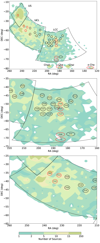
Figure 1: Density map of the known (stellar) Sco-Cen members in DECam fields observed in May 2015. Red circles mark fields observed in both 2013 and 2015 while black circles were only observed in 2015. The top plot shows all of Sco-Cen and the fields we observed while the middle and lower panels show UCL and LCC respectively, along with the names of the fields used in our survey (field names populate the “OBJECT” key in the DECam FITS headers and are listed for each source in our catalog).

Our survey uses observations taken with DECam, mounted at the prime focus of the Blanco 4-m telescope at Cerro Tololo Inter-American Observatory (CTIO). DECam has 60 or 61 2048$\times$4096 functioning CCDs (depending on the observation date) and a field of view (FOV) of $\sim$3 deg² (2.2 deg wide) with a 0.263 arcsec pixel^-1 resolution. Gaps between the rows and columns of CCDs are 201 pix ($\sim$53 arcsec) and 153 pix ($\sim$40.3 arcsec) respectively. The images were taken in the $izY$ filters (775, 925, 1000 nm central wavelengths respectively), where the $iz$ filters were designed to closely match SDSS $iz$ (762 nm, 913 nm respectively). Our images were taken during two separate runs: the first run on 2013 May 29-30, which was only photometric for 5 hours and a second run on 2015 May 26-27. We observed a total of 6 photometric fields in 2013 and 29 in 2015 (see Figure 1). Each science image was observed in each band for 7s, then 3 exposures using the same pointing in each filter as follows: 200s in $i$ and 30s in $zY$. For photometric calibration we also observed three SDSS fields centered at: (14:42:00,-00:04:50), (12:27:00,-00:04:50), (10:48:00,00:00:10). The calibration fields were observed once every 1-2 hours for 30s in $i$ and 15s in $zY$. The mean completeness limits for each filter are $i=21.8$, $z=20.4$, $Y=18.6$ mag with saturation at $i=12.6$, $z=12.4$, and $Y=11.6$ mag.

The DECam images were reduced using the steps described in more detail in Appendix A. Briefly, using the InstCal images produced by the DECam community Pipeline (Valdes et al., 2014), we stack the longer exposures in $izY$ individually for each CCD and combine the catalogs generated from the stacks with the 7s exposure catalogs in all three filters to create a master catalog of point sources. PSF photometry is performed on the individual CCDs and calibrated to the SDSS AB system (for $iz$) and UKIDSS Vega system (for $Y$) using the standard fields. An astrometric solution is derived for each CCD in 2013 and 2015 and the 6 fields observed in both epochs are compared to generate relative proper motions that are calibrated to Gaia observations (referred to as DECam proper motions for the remainder of this paper). All of the fields also have proper motions calculated by matching our catalog to the 2MASS (Skrutskie et al., 2006), DENIS (Epchtein et al., 1997), AllWISE (Wright et al., 2010), UCAC4 (Zacharias et al., 2013), USNOB 1.0 (Monet et al., 2003), and GAIA (Gaia Collaboration et al., 2016) catalogs (referred to as Sky proper motions for the remainder of this paper). Fields observed in both epochs have both DECam and Sky proper motions recorded in the final catalog.

3 SCOCENSUS Catalogs

The total number of point sources detected in the 2013 and 2015 DECam imagery was over 11 million, with $\sim$5 million sources detected in both $i$ and $z$ and $\sim$3 million detected in both $z$ and $Y$. For each source the full catalog contains the epoch, position, DECam $izY$ photometry, 2MASS $JHK_{s}$ photometry (when available), AllWISE photometry (when available), DENIS $IJK$ photometry (when available), Sky proper motions (see previous section), DECam proper motions (when available, see previous section), the name of the observed field, Sco-Cen subgroup of the field (Upper Sco, UCL, LCC), and various flags created in the execution of the pipeline. The full catalog is available on Vizier.

Our fields were taken at a variety of Galactic latitudes, causing the color-magnitude diagrams (CMDs) to suffer from increased reddeding at lower Galactic latitudes. In addition to the spatial separation between UCL and LCC, the clustering of ages illustrated in Figure 9 from Pecaut & Mamajek (2016) results in potentially different distances and ages for all of our DECam fields. As a result we perform our candidate selection on each field individually to select candidates and calculate their estimated properties.

3.1 Candidates

Candidate members in UCL and LCC are selected using photometric and kinematic cuts that appear to have a false positive rate of $\sim 5-6\%$. We first use our DECam photometry to select objects near isochrones created using the Baraffe et al. (2015) stellar evolution models calibrated with Allard et al. (2011) atmospheric models, eliminating all but $4.7\times 10^{-2}$% of the sources in our catalog. Next we select objects with proper motions consistent with Chen et al. (2011) estimates of UCL and LCC group velocities, dividing our candidates into “best”, “good”, and “no pm” categories based on their observed proper motions. Finally we use 2MASS photometry to remove M giants with similar $izY$ colors that occupy a different region in ($H-K_{s}$,$J-H$) color-color space than YLMOs (Cruz et al., 2009). The definition of our proper motion categories, a more thorough explanation of how we built our models and the procedure used to select candidates is described in Appendix B.

Once all of our cuts have been made, we are left with 118 best candidates in the fields observed in 2013 and 2015 and 348 more good candidates as defined in Appendix B. While our full catalog of candidates contains many more fields, we present a few tables with the most important fields for each candidate. Table LABEL:tab:candidates lists the observed properties for all of the candidates.

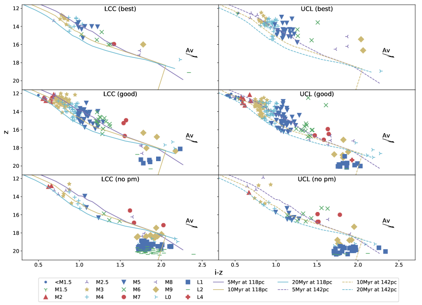
Figure 2: YLMO candidates in LCC (left) and UCL (right). Error bars have been omitted for clarity, as the errors for most sources are smaller than the size of the markers. The top row shows the sources observed in two epochs with proper motions and photometry consistent with membership in Sco-Cen. The middle row shows sources observed in only 2015 with proper motions and photometry consistent with Sco-Cen membership, and the bottom row shows objects observed in 2015 that are photometrically consistent with Sco-Cen membership but are not found in any existing all-sky catalog, and thus have no proper motion estimates. Due to a lack of proper motions and limited photometric bands (missing $JHK_{s}$ photometry makes it more difficult to rule out giants), most of the objects in the bottom row are expected to be non-members. See Appendix B for further information.

As described in Appendix B, we also derived estimates for the effective temperature, extinction, spectral type, and mass for all of the candidates. Table 1 shows the derived properties for all of the candidates in UCL and LCC. We use lower case letters and the heading “Spectral Template” to make it clear that our spectral types are photometric estimates and not based on observed spectra (however in Section 6 we show that our estimates appear to be within a subtype for all candidates that have observed spectra).

Table 1: Derived properties of low mass stellar and substellar candidates in UCL and LCC

id	$T_{eff}$	Av	Spectral	Mass
	(K)		Template	($M_{\odot}$)
Moolekamp 1	$3163^{+103}_{-103}$	$0.16^{+0.19}_{-0.11}$	m4	$0.16^{+0.04}_{-0.05}$
Moolekamp 2	$2763^{+73}_{-73}$	$0.15^{+0.19}_{-0.10}$	m6	$0.05^{+0.01}_{-0.01}$
Moolekamp 3	$3106^{+92}_{-92}$	$0.15^{+0.20}_{-0.09}$	m5	$0.13^{+0.06}_{-0.03}$
Moolekamp 4	$3081^{+71}_{-71}$	$0.19^{+0.19}_{-0.12}$	m5	$0.11^{+0.04}_{-0.01}$
Moolekamp 5	$2959^{+72}_{-72}$	$0.17^{+0.18}_{-0.11}$	m5	$0.07^{+0.02}_{-0.01}$

• Only the first five rows are shown; this table is available in its entirety in the electronic version of the journal

4 Luminosity and Mass Functions

4.1 Luminosity Functions in UCL and LCC

Before calculating the IMF it can be useful to first estimate the luminosity function (LF), which describes the distribution of absolute magnitudes of the observed cluster or association (the term “luminosity function” is a bit misleading as historically it has been a distribution and not a function that is calculated). For much of the 20th century, the calculation of absolute magnitudes for low mass stars in the field proved to be quite challenging (distance estimates based on parallax were accurate to $\lesssim$10 pc), leading to much disagreement and controversy regarding the abundance of M dwarfs and the shape of the LF (Reid & Hawley, 2005). For young clusters and associations, both the distance to the groups and approximate reddening are known from astrometric and spectral observations of their stellar populations and make the conversion of apparent to absolute magnitudes somewhat simpler.

This does not mean that the low mass LF is universal, as it can change dramatically in time. Allen et al. (2003) investigated how the LF changes in clusters as they age, simulating a cluster pulled from a Kroupa (2002) IMF and allowing the low mass stars and substellar objects to evolve using the Burrows et al. (2001) models. As brown dwarfs cease deuterium burning and begin to rapidly cool, their luminosities decrease and distinct peaks in the group’s luminosity function can be seen as brown dwarfs transition from star-like luminosities to planet-like luminosities (see Allen et al. 2003 for a description of the evolution of cluster luminosity up to 1 Gyr). Allen et al. (2003) compared observations of several young clusters and associations to simulations which exhibit agreement with a Kroupa-like power-law, with a low mass $\Gamma=0.5$. Rather than run a new set of stellar evolutionary models, we use the Ardila et al. (2000) observations of Upper Sco modeled by Allen et al. (2003) as a tool for comparison: due to the similar ages of Upper Sco, UCL, and LCC, as well as their origin in the same molecular cloud, there should not be a significant difference between their LF’s. The main source of error in our LF are uncertainties in the distance to the objects, where a difference between 100 pc and 200 pc gives a systematic error of $\sim$1.5 mag, while the mean uncertainty in apparent magnitude is $\sim$0.02 mag. To convert the Ardila et al. (2000) $I$ to SDSS $i$ we use the transformation $i-I=(0.247\textpm 0.003)*(R-I)$ from Jordi et al. (2006) (see Figure 3).

We also compare the $M_{J}$ luminosity function from UCL, LCC, and their combined LF in Figure 4. Here we see the importance in having a large number of sources to create the low mass LF in a meaningful way, as the $M_{J}$ LF for LCC sources observed in two epochs only has 38 best sources and is noticeably different from the UCL and combined LFs. Once a reasonable number of sources is included in the sample (for example the 80 best UCL sources) the LF has the same approximate shape regardless of the number of sources added or cuts used. This shows that while individual fields might show slight variations, the underlying mass function inferred from the LF is likely to be the same in all of Sco-Cen (Upper Sco, UCL and LCC).

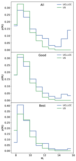
Figure 3: Comparison between the luminosity function measured using our UCL and LCC data and the luminosity function using Ardila et al. (2000) observations of Upper Sco, normalized so that each distribution has the same total number of stars in the magnitude range available to Ardila et al. (2000) (our observation range covers slightly brighter to significantly fainter objects), using the Jordi et al. (2006) offset of $0.329+0.29(R-I)$ to convert Ardila et al. (2000)’s $I$ to our SDSS calibrated $i$ magnitudes. The $x$ axis displays the absolute magnitude in $i$, calculated assuming distances of 145 pc, 142 pc, and 118 pc for Upper Sco, UCL, and LCC, respectively. The y axis is the fraction of the total sources in the group (or in this case subset of UCL, LCC, or Upper Sco) in a given luminosity bin. We see that all three sets of proper motion cuts described in Appendix B show excellent agreement with the Upper Sco luminosity function, although they do deviate from each other for sources fainter than 14 mag. We expect that this is due to interlopers in the top panel with no or poorly constrained proper motions.

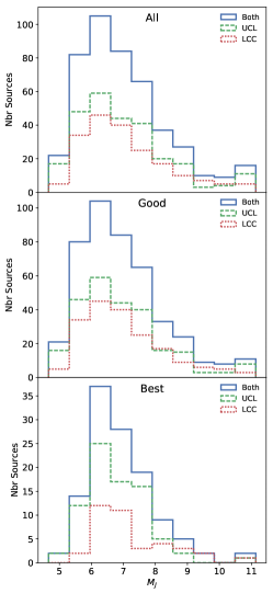
Figure 4: Comparison of the M_J luminosity functions for LCC, UCL, and their combined luminosity function. The top plot shows all of the candidates objects, the middle combines the good and best sources, and the bottom plot shows only the best sources.

4.2 Mass Functions in UCL and LCC

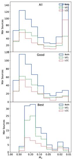
Figure 5: We compare the mass functions in UCL, LCC, and a combination of the two using the proper motion cuts. The best sample contains enough sources to likely be the most representative of the actual IMF and future work will investigate the anomalous excess in the good and “all” plots for $m<20M_{\textrm{Jup}}$.

Calculation of the mass function (MF) from a set of photometric observations is more prone to error/uncertainty as it cannot be calculated without the aid of evolutionary models. This is further complicated by known errors with most stellar evolution codes, which tend to predict younger ages for lower mass objects and older ages for higher mass stars (Bell et al., 2012; Pecaut et al., 2012; Kraus et al., 2015; David et al., 2016). Rizzuto et al. (2016) analyzed a population of G,K, and M-type binary systems in Upper Scorpius and estimated that while the G-type systems were consistent with $\sim$11 Myr ages, M dwarfs appeared to be much younger ($\sim$7 Myr), corresponding to an effective temperature over prediction of 100-300 K. They also note that while the majority of B-type stars in Upper Scorpius were consistent with an age of $\sim$11 Myr, a few B-type stars show evidence of being 6-9 Myr younger.

Pecaut & Mamajek (2016) analyzed the ages of 657 F, G, K, and M-type members in all three Sco-Cen subgroups. Instead of predicting the ages using a set of model isochrones, they use the observed luminosities of the stars to calculate an empirical isochrone. They assume that each subgroup has some mean age with an intrinsic age spread around the mean, corresponding to different star-forming events. Younger stars are more luminous, so for a given spectral type they equate the mean luminosity with the mean age and interpret a spread in luminosities as a spread in ages. This gave them an empirical isochrone, which they used to generate a chronological plot of the age distribution for the entire Sco-Cen association. As predicted by Rizzuto et al. (2016), they show that lower mass objects appear to have their ages underestimated by stellar and substellar models.

If the results of Rizzuto et al. (2016) and Pecaut & Mamajek (2016) are correct, the locations of our sources in color magnitude diagrams should make them appear younger (as a whole) than the mean ages of UCL and LCC. Looking back at Figure 2 we see that indeed they do, where very few objects apear older than 15 Myr, with a mean inferred isochronal age between 2-10 Myr and fainter sources appearing much younger than even the 1 Myr isochrone(not shown in Figure 2)). Feiden (2016) investigated the effects of magnetic fields on convection for a population of A-M stars in Upper Scorpius. He showed that simulations introducing a magnetic perturbation, with a peak magnetic energy density much less than the thermal energy density, inhibits convection in low mass stars, causing them to appear more luminous. Due to shrinking convection zones as the mass of a star increases, this effect decreases and all but vanishes for stars with masses above $\sim 1.2$ $M_{\odot}$.

Because Feiden’s models have a lower mass limit of 85 M${}_{\textrm{Jup}}$, there are no models covering our observed mass range that accurately match observations. For this reason one has to be careful how to interpret the results of our MCMC predictions of mass, age, and distance and respect the various caveats inherent within. The reason for calculating them at all is that the magnitudes in the BT-Settl atmospheric models (Allard et al., 2011) are given at the stellar surface, requiring an isochrone (or set of isochrones) to calibrate the radius at each T${}_{\textrm{eff}}$ to calculate an absolute magnitude. One might argue that fitting distance, age, A_V, mass, and $\log(g)$ is overkill just to get an effective temperature, but spectral results to be published in Moolekamp et al. (prep) following up on a few dozen objects show that our predictions of spectral class are accurate to within $\pm\frac{1}{2}$ a subclass (for most sources). Examination of Figure 2 also shows that predicted spectral classes for most sources transition smoothly from hotter to cooler sources for objects with measured proper motions and $JHK_{s}$ photometry. Unfortunately, slight changes in T${}_{\textrm{eff}}$, distance, mass, and age, create degeneracies in the photometry, making it much more difficult to calculate them with any degree of certainty.

Even if we were to have a set of models that could reasonably predict the mass of our sources using photometry alone, higher order corrections due to binary fraction and dynamical evolution can have a noticeable impact on the IMF, making a much more thorough study necessary to properly model the IMF in UCL and LCC. Instead we present preliminary results from our BHAC2015 (Baraffe et al., 2015) model comparisons in Figure 5 to qualitatively display the approximate MF using the best, good, and entire candidate lists (see Appendix B.2). Future work that includes spectroscopic observations and a mass-luminosity relation derived from spectroscopic binaries in Upper Scorpius will allow us to provide a more thorough estimate (Moolekamp et al., prep).

5 IR Excess in UCL and LCC

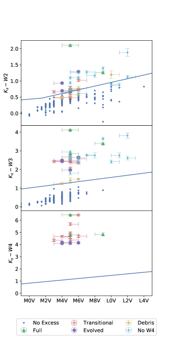
Figure 6: Color-color diagrams for 2MASS $K_{S}$ and AllWISE $W1$, $W2$, $W3$, and $W4$ compared with estimated T${}_{\textrm{eff}}$, compared to Baraffe et al. (2015) isochrones using the BT-Settl (Allard et al., 2011) atmospheric models (black solid line) and 2$\sigma$ cutoff (blue dashed line). Candidates have been categorized based on the observational criteria in Luhman & Mamajek (2012), with small dots representing sources that do not show excess indicative of circum-primary disks. Sources with error bars show an excess in all three WISE colors and are likely to have circum-primary disks (see Table 3).

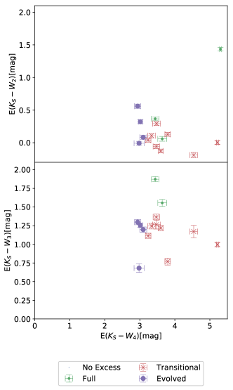
Figure 7: Color excess and estimated disk types for all objects with excess in all WISE bands

As mentioned in the introduction, 10-20 Myr is an important timeframe in the lifetime of circum-primary disks, where stars (and presumably substellar objects) can have disks in a wide range of evolutionary stages. For objects with optical spectra, the detection of disks can be performed by calculating the equivalent width of the H$\alpha$ feature (Barrado y Navascués & Martín, 2003) and using it to classify a star as a Classical or Weak T-Tauri Star (CTTS or WTTS). It is also possible to identify disks using IR photometry, where Espaillat et al. (2012) used Spitzer IRAC (Fazio et al., 2004) and WISE photometry to distinguish between full, transitional, evolved, debris, and no circumstellar disks. Photometric classification of disks uses IR photometry compared to K-band photometry, which is short enough to resemble photospheric flux and long enough to suffer from limited extinction, to estimate the excess color in a source compared to photospheric colors.

Table 2: Infrared excess and disk fractions for K-type and M-type member of UCL and LCC. Using the criteria described in Section 5, we show the fraction of K-type members from Pecaut & Mamajek (2016) and compare them to the M-type members in this paper. Note that the Pecaut & Mamajek (2016) sources have been spectroscopically confirmed with EW(H$\alpha$ measurements) while the M-type stars from this survey are candidate members with estimated spectral types and our estimated disk fractions should be viewed as lower bounds, as many of our sources do not have reliable $W3$ and $W4$ photometry (due to the small number of sources with reliable $W4$ photometry we do not include the percentage of sources with excess in $W4$ to avoid confusion).

Band/Disk Type	UCL		LCC
	K-type	M-type	K-type	M-type
W2	11/157 (7.0%)	14/246 (5.7%)	5/119 (4.2%)	12/175 (6.9%)
W3	9/157 (5.7%)	16/139 (11.5%)	4/118 (3.4%)	11/129 (13.2%)
W4	44/72	8/8	29/86	7/7
Full	8/157 (5.1%)	3/267 (1.1%)	4/118 (3.4%)	0/199 (0.0%)
Transitional	0/157 (0.0%)	4/267 (1.5%)	0/118 (0.0%)	4/199 (2.0%)
Evolved	1/157 (0.6%)	1/267 (0.4%)	0/118 (0.0%)	3/199 (1.5%)
Debris	24/157 (15.2%)	5/267 (1.9%)	14/118 (11.9%)	1/199 (0.5%)
No W4	–	6/267 (2.2%)	–	9/199 (4.5%)

Table 3: AllWISE photometry for sources with 2$\sigma$ excess in $K_{s}-W1$ $K_{s}-W2$, $K_{s}-W3$, $K_{s}-W4$ colors. Sources marked with a $\dagger$ show an excess in that color.

id	AllWISE id	Spectral Template	$K_{S}-W2$	$K_{S}-W3$	$K_{S}-W4$	Disk Type
			(mag)	(mag)	(mag)
Moolekamp 2	J121551.25-493734.8	M6	$0.36\pm 0.04$	$2.30\pm 0.07$$\dagger$	–	No W4
Moolekamp 13	J121610.32-521919.7	M6	$0.56\pm 0.03$$\dagger$	$1.92\pm 0.04$$\dagger$	$3.42\pm 0.09$$\dagger$	Evolved
Moolekamp 17	J122351.30-522413.4	M7	$0.61\pm 0.04$$\dagger$	$2.11\pm 0.05$$\dagger$	–	No W4
Moolekamp 45	J121925.27-562049.9	L2	$0.76\pm 0.11$$\dagger$	$2.69\pm 0.14$$\dagger$	–	No W4
Moolekamp 49	J122242.29-563611.5	M5	$0.41\pm 0.03$$\dagger$	$2.11\pm 0.03$$\dagger$	$4.09\pm 0.08$$\dagger$	Transitional
Moolekamp 73	J152649.42-355829.2	M5	$0.48\pm 0.03$$\dagger$	$2.72\pm 0.06$$\dagger$	–	No W4
Moolekamp 76	J152700.55-360113.3	M5	$0.21\pm 0.04$	$1.08\pm 0.15$$\dagger$	–	Debris
Moolekamp 91	J152842.76-362618.0	M5	$0.27\pm 0.04$	$2.26\pm 0.08$$\dagger$	$5.48\pm 0.11$$\dagger$	Transitional
Moolekamp 105	J152907.03-365551.8	M5	$0.46\pm 0.03$$\dagger$	–	–	Debris
Moolekamp 121	J153516.17-393746.3	L0	$0.70\pm 0.12$$\dagger$	–	–	Debris
Moolekamp 153	J154609.72-344827.9	M4	$0.22\pm 0.03$	$0.99\pm 0.05$$\dagger$	–	Debris
Moolekamp 167	J154745.85-351319.7	M5	$0.38\pm 0.03$	$1.70\pm 0.06$$\dagger$	$3.85\pm 0.14$$\dagger$	Evolved
Moolekamp 169	J154756.93-351434.9	M5	$0.83\pm 0.03$$\dagger$	$2.85\pm 0.02$$\dagger$	$5.17\pm 0.02$$\dagger$	Full
Moolekamp 180	J154816.78-352321.3	M9	$0.73\pm 0.03$$\dagger$	$2.86\pm 0.04$$\dagger$	$4.31\pm 0.11$$\dagger$	Full
Moolekamp 181	J154826.33-352544.3	M9	$0.80\pm 0.05$$\dagger$	$3.06\pm 0.06$$\dagger$	–	No W4
Moolekamp 185	J154525.41-353431.5	M5	$0.39\pm 0.03$$\dagger$	$2.45\pm 0.05$$\dagger$	–	No W4
Moolekamp 200	J154806.22-351548.5	M6	$0.41\pm 0.03$$\dagger$	$2.03\pm 0.03$$\dagger$	$6.11\pm 0.03$$\dagger$	Transitional
Moolekamp 224	J125232.27-563053.1	L0	$0.43\pm 0.04$	$1.96\pm 0.09$$\dagger$	–	No W4
Moolekamp 225	J124541.67-564312.0	M6	$0.57\pm 0.03$$\dagger$	$2.16\pm 0.06$$\dagger$	$4.24\pm 0.11$$\dagger$	Transitional
Moolekamp 248	J125423.62-531111.2	M4	$0.26\pm 0.03$	$2.23\pm 0.03$$\dagger$	$4.45\pm 0.07$$\dagger$	Transitional
Moolekamp 337	J123410.32-513042.3	L1	$0.64\pm 0.06$	$2.52\pm 0.13$$\dagger$	–	No W4
Moolekamp 347	J122651.99-523618.1	L2	$0.78\pm 0.05$$\dagger$	$2.27\pm 0.10$$\dagger$	–	No W4
Moolekamp 366	J123642.32-503613.2	M6	$0.57\pm 0.04$$\dagger$	$1.96\pm 0.06$$\dagger$	–	No W4
Moolekamp 369	J123938.39-504240.4	M6	$0.53\pm 0.04$$\dagger$	$1.84\pm 0.05$$\dagger$	–	No W4
Moolekamp 392	J120808.89-502655.9	M4	$0.43\pm 0.03$$\dagger$	$2.16\pm 0.04$$\dagger$	$3.91\pm 0.10$$\dagger$	Evolved
Moolekamp 396	J120624.51-505415.3	M4	$0.46\pm 0.03$$\dagger$	$2.02\pm 0.03$$\dagger$	$3.62\pm 0.06$$\dagger$	Evolved
Moolekamp 414	J122556.71-472154.7	M6	$0.31\pm 0.03$	$1.20\pm 0.05$$\dagger$	–	Debris
Moolekamp 449	J130515.48-502438.9	M5	$0.57\pm 0.03$$\dagger$	$2.11\pm 0.05$$\dagger$	–	No W4
Moolekamp 466	J131107.55-445553.1	M5	$0.43\pm 0.03$$\dagger$	$1.70\pm 0.05$$\dagger$	$4.57\pm 0.08$$\dagger$	Transitional
Moolekamp 524	J150703.47-440859.3	M5	$0.37\pm 0.04$$\dagger$	$1.43\pm 0.10$$\dagger$	–	No W4
Moolekamp 590	J143000.21-453045.3	M8	$0.55\pm 0.05$$\dagger$	$2.14\pm 0.14$$\dagger$	–	No W4
Moolekamp 597	J142844.81-455718.0	M6	$0.52\pm 0.06$$\dagger$	–	–	Debris
Moolekamp 602	J142429.95-462142.1	M3	$0.36\pm 0.03$$\dagger$	$2.12\pm 0.04$$\dagger$	$4.05\pm 0.11$$\dagger$	Transitional
Moolekamp 619	J140445.33-432348.4	M5	$0.52\pm 0.03$$\dagger$	$2.10\pm 0.05$$\dagger$	–	No W4
Moolekamp 630	J140020.08-440317.6	M5	$0.42\pm 0.04$$\dagger$	$2.54\pm 0.05$$\dagger$	$4.48\pm 0.13$$\dagger$	Full
Moolekamp 652	J140635.06-392640.9	M5	$0.34\pm 0.03$	$2.39\pm 0.04$$\dagger$	$4.34\pm 0.09$$\dagger$	Transitional

The X-ray and kinematic search of Sco-Cen performed by Mamajek et al. (2002) used 2MASS $K_{s}$-band IR excess and H$\alpha$ emission to search for accretion disks around K-type members of UCL and LCC, identifying only a single source out of 110 stellar candidates that displayed evidence of an optically thick accretion disk. More recently Pecaut & Mamajek (2016) used the Espaillat et al. (2012) classification scheme, combined with the Luhman & Mamajek (2012) observational criteria to estimate the disk fraction for K-type stars in UCL and LCC (they also had a few early M stars in their sample but not enough to provide a reasonable estimate of the disk fraction), where they identify 12 out of 275 stars K stars with a full disk, none with a transitional disk, and a single evolved disk. If estimates that lower mass stars can possess longer lived disks is correct, we should expect to find more disks around the M and L dwarfs in our sample.

We perform an analysis similar to Pecaut & Mamajek (2016), using the Espaillat et al. (2012) classification criteria and the Luhman & Mamajek (2012) observational criteria. $K_{S}$ photometry is taken from the 2MASS catalog and compared to AllWISE $W2$, $W3$, and $W4$ (in this mass regime excess in $K_{S}-W1$ due to the presence of a disk is negligible) for each source. We reject all sources with photometric errors $>0.2$ mag and visually inspect all remaining sources for nearby neighbors and other contaminants. Of the 466 good or best sources: 421 have reliable $W2$ photometry, 268 have $W3$, and only 15 have $W4$ photometry with errors $<0.2$ and no local contaminants. We characterize IR excess in our sample using the same criteria as Luhman & Mamajek (2012) used for Upper Sco, where an excess in $K_{S}-W2$ is defined by the lines connecting (B0, 0.19), (K0, 0.22), (M1.5, 0.47), and (M8.5, 0.87), $K_{S}-W3$ excess is defined by (B0, 0.18), (G8, 0.33), and (M9, 1.52), and $K_{S}-W4$ excess is bounded by (B0, 0.11), (K6, 0.57), and (M9, 1.4) (because some sources in our sample have estimated spectral types later than M9, we interpolate the last line segment for each color to L5). This is slightly different than the criteria used in Pecaut & Mamajek (2016), so we also re-analyze their sample of K stars in UCL and LCC for a more accurate comparison with our M dwarf candidates. Using the same excess boundaries as Luhman & Mamajek (2012) also allows us to use the same criteria to classify disks, where we classify a disk as “full” if E($K_{S}-W3$) > 1.5 and E($K_{S}-W4$) > 3.2, “transitional” if E($K_{S}-W3$) < 1.5 and E($K_{S}-W4$) > 3.2, “evolved” if E($K_{2}-W3$) > 0.5 and E($K_{S}-W4$) < 3.2, and “debris” if E($K_{S}-W3$) < 0.5 and E($K_{S}-W4$) < 3.2. Most of our sources do not have reliable $W4$ photometry, so we add an additional classification for our candidates with $K_{S}-W3$ > 0.5 but no reliable $W4$ photometry as “no $W4$”. Table 3 shows the $K_{s}-Wn$ colors for candidates showing an IR excess in one or more of the bands, with a $\dagger$ marking colors that show an excess from estimated photospheric colors, and the estimated disk type of each source using the criteria stated above.

Table 2 shows a comparison of IR excess and disk fractions from our survey of M dwarfs in UCL and LCC compared to Pecaut & Mamajek (2016) observations of K-type stars in the same subgroups (while the Pecaut & Mamajek (2016) sample contains roughly the same number of objects, due to stellar populations their sample is obtained over a much larger region of UCL and LCC). We find comparable IR excess in $W2$ for K- and M-type sources and while we seem to find a higher fraction of sources with $W3$ and $W4$ excess, we are biased to find a higher percentage of objects with excess since lower mass objects are less likely to have reliable photometry in those bands without excess flux. While we appear to find more transitional and evolved disks and fewer full and debris disks, excess calculations are highly dependent on spectral type and proper spectral classifications might correct our results. We expect to revisit this issue in more detail in a future paper once we have spectrally classified a large portion of our candidates.

6 Mass Segregation in $\eta$ Cha

In addition to the main subgroups of Sco-Cen: Upper Sco, UCL, and LCC, there are a number of nearby clusters kinematically linked to the Sco-Cen star-forming complex. Among these is the 11$\pm$3 Myr old $\eta$ Cha cluster (Bell et al., 2015), first discovered by Mamajek et al. (1999) using X-ray detections from ROSAT. At a distance of $\sim$95 pc, $\eta$ Cha has higher proper motions than the main Sco-Cen subgroups and has negligible reddening (Av$\sim$0 mag), making it easier to kinematically and photometrically select members. It is also a relatively compact cluster, almost entirely contained in a single DECam image (see Figure 1), with only 18 known members (Becker et al., 2013).

Table 4: Members detected in $\eta$ Cha by the SCOCENSUS pipeline. The Spectral Type is the spectral type as given in Luhman (2004), while the Estimated Sp Type Range is the predicted range of spectral types using MCMC and the Spectral Template is the most likely spectral type.

SCOCENSUS	2MASS	RECX	SpT	Estimated SpT Range	Spec. Template
100-9452	J08440914-7833457	16	M5.75	M6-M6	m6
100-24176	J08385150-7916136	17	M5.25	M5-M6	m5
100-40810	J08413030-7853064	14	M4.75	M4-M5	m5

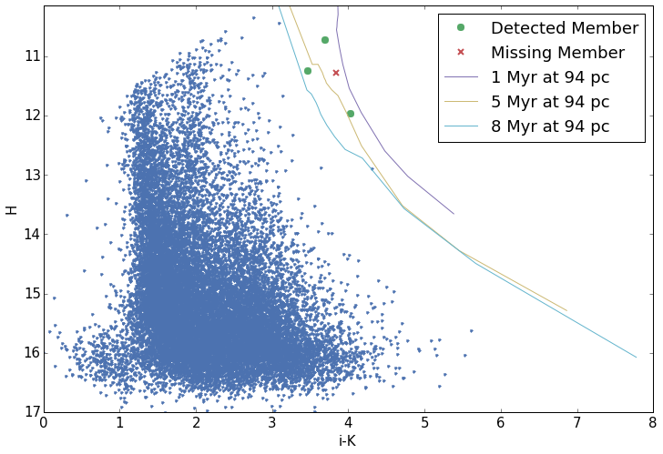
Figure 8: Color magnitude diagram for $\eta$ Cha field (F100). The green circles mark the $\eta$ Cha members that we detected and the red x is an M dwarf that was in between the CCD gaps in our 2015 images (the point is plotted using the magnitudes from Luhman (2004)). The predicted age range of $\eta$ Cha is $\sim$6-8 Myr but based on the discussion in Section 4.2, it seems likely that $\eta$ Cha is closer to the 11 Myr age predicted by Bell et al. (2015), since the Baraffe et al. (2015) models tend to underpredict the age of low mass stars.

Previous surveys of the region performed by Luhman (2004); Song et al. (2004); Lyo et al. (2006) have searched for substellar objects in $\eta$ Cha but no objects $\lesssim$0.1 M_⊙ were found within 1.5^∘. Murphy et al. (2010) extended the search in a wider survey with a radius of 5.5^∘, finding 4 “probable” and 3 “possible” members with estimated masses between 0.08 and 0.3 M_⊙. Becker et al. (2013) noted these results and attempted to reverse engineer the dynamical evolution of $\eta$ Cha assuming a universal IMF and the known positions of current members. By running a number of N body simulations using several sets of initial conditions, they concluded that it is very unlikely that $\eta$ Cha’s current configuration, with high mass stars concentrated toward the center and low mass stars in a surrounding halo, occurred by dynamical processes alone. Instead they conclude that the mass segregation in the region is most likely primordial.

To investigate this claim we took a single set of DECam images centered on $\eta$ Cha (field F100). We ran the images through the same pipeline used for our UCL and LCC fields and detected three M dwarfs: 2MASS J08440914-7833457, 2MASS J08385150-7916136, and 2MASS J08413030-7853064, all of which were detected by Luhman (2004) (they also detect an additional fourth M-dwarf that is not in our catalog, see Figure 8). The missing M dwarf fell between the gaps of our detector, as we did not dither our images in order to stack individual CCD’s. We did not detect any new brown dwarfs down to magnitudes $i=21.2$, $z=20.3$, $Y=18.6$ mag, including objects fainter than 2MASS and AllWISE, verifying that there are not likely to be any brown dwarfs within a 1.1^∘ radius of $\eta$ Cha.

This field also served as a valuable crosscheck for our pipeline. All three M dwarfs in our catalog were flagged as $\eta$ Cha candidates by our pipeline and the spectral types of the objects fall within the ranges of our predictions (see Table 4). We should note that these would be flagged as good and not best by our pipeline, since none of the sources have DECam and sky proper motions that are both consistent with Sco-Cen (two of the sources have underestimated $\mu_{\alpha}$ and the other fell between the detector gaps in 2013 and does not have a DECam proper motion). The detection and proper spectral typing of all of the known objects in our field of view serves as evidence that our photometry and astrometry are well calibrated.

7 Conclusion

We presented the results of a small scale $izY$ survey covering $\sim$87 deg² in the UCL and LCC subgroups of the Scorpius Centaurus OB association to search for low mass stars and substellar objects. Our observations include a catalog with over 11 million point sources and 466 candidate members of Sco-Cen, including an estimated 80-100 brown dwarfs detected in LCC and UCL based on isochronal models.

Our observations add to the growing body of evidence suggesting that models of PMS stars and young substellar objects are missing key physical processes that underestimate their luminosity in the near IR, causing them to predict much younger ages for lower mass objects. Nevertheless we show that the luminosity function in UCL and LCC is nearly identical to observations made by Ardila et al. (2000) in Upper Sco and that the IMF is consistent with observations of other young clusters.

We see IR excess indicative of circum-primary disks, with similar disk fractions to higher mass K-type stars presented in Pecaut & Mamajek (2016). There is some discrepancy in the exact classification, where we find more transitional and evolved disks and fewer full and debris disk. Spectral classification of our objects will reveal if this is a real effect or a result of small differences between our estimated spectral templates and the objects true spectral types.

While the initial results of this survey are encouraging, there is still much work to be done. Follow-up photometry is needed for objects below the completion limit of GAIA, 2MASS, and AllWISE to calculate proper motions for candidate L dwarfs ($m\lesssim$10-15 $M_{\textrm{Jup}}$). Using longer exposures in $zY$ bands it should also be possible to detect later L dwarfs if they exist in isolation, however in the absence of faint all-sky catalogs it will require multiple epoch photometry to generate reasonable proper motions (for example LSST). Follow-up photometry in $JHK_{s}$ will also allow the removal of giant interlopers in magnitude regions too faint for 2MASS detections. This will provide valuable constraints to our photometrically selected L dwarf candidates to allow us to probe the substellar IMF in a currently unexplored mass regime. Spectroscopic followup of our candidates has already begun and will help us understand any biases in our candidate selection and estimations of spectral type and mass, which can be used to derive a more precise model of the IMF in Sco-Cen.

Appendix A Image Reduction Pipeline

When this survey was started there was no reliable pipeline to reduce such a large volume of data that was also tunable for the precise measurements required to accurately calculate proper motions and PSF photometry in the galactic plane. In the meantime the LSST software stack has reached a higher level of maturity, especially with the addition of the new scarlet deblender (Melchior et al., prep), and is likely to outperform the data reduction described in this appendix. This appendix is still included to describe the reduction used in this paper and educate the reader curious about how to reduce survey data at scale.

The computational framework needed to conduct our survey consists of a collection of python libraries. Many of these libraries were developed by the the first author but extensive use was made of astropy (Astropy Collaboration et al., 2013) and its affiliated packages (including contributions to those packages made by the author). Because many of the challenges we faced will confront other groups both in the present and future, we decided to make our software open source and more general than necessary for our own use, but not as general as possible. This was done to save time and because anyone performing interesting research is likely to need slight modifications to the codes anyway and will likely need to fork our code and use their own version. The main framework and execution of the pipeline is handled by the datapyp package , written by the first author to enable users to run large pipelines so that when the inevitable crash occurs, users can easily modify the code and restart the pipeline at any previous (or future) step. It is also possible to run subsets of a pipeline, making it much easier to make improvements to image reduction and analysis portions of the pipeline. The vast majority of our pipeline is available as the astropyp package , which contains the general high-level image reduction procedures that might be useful to a wide variety of astronomers. Functions more specific to our own research can be found in the scocensus (SCOrpius CENtaurus SUbstellar Survey) package, which includes all of the scripts used to run our pipeline and select substellar objects from our final catalog (this package is currently private because our data is already public, but the software will be made public as well once our survey is complete).

A.1 Astrometry and Stacking

The limiting factor in calculating sky positions of DECam sources is the accuracy of the reference catalog used to generate the astrometric solution. While DECam has better than 20 mas astrometric precision (Bernstein, 2015), until the recent GAIA DR1 release (Gaia Collaboration et al., 2016), the best all-sky catalog that covered Sco-Cen in the magnitude range probed in exposures ranging from a few seconds to several minutes was 2MASS , which has >100 mas uncertainty in RA and DEC. Since the size of a DECam pixel is $\sim$262.7 mas/pixel, the error is nearly half a pixel, causing stacked images to have unnecessary noise (see Figure 9). Since our initial analysis, GAIA DR1 was published, however due to the success of our astrometric solution we have not modified our pipeline other than to use GAIA in the place of 2MASS as our reference catalog.

To improve the calculation of our proper motions we realized that it would be necessary to create our own astrometric solution to align exposures based on their image coordinates, not their world coordinates (see Section A.3). This solution is also useful for stacking our exposures as it allows us to create stacks with much smaller positional errors.

The basic astrometric solution is very similar to the one implemented in SCAMP, using the transformations described in Kaiser et al. (1999):

$$x_{r} =\sum_{l=0}^{l=N}\sum_{m=0}^{m=l}a_{lm}x^{l}y^{m}$$ (1)

$$y_{r} =\sum_{l=0}^{l=N}\sum_{m=0}^{m=l}b_{lm}y^{l}x^{m}$$ (2)

where $x_{r},y_{r}$ are the reprojected positions of a source (which can be any orthogonal 2D coordinate system), $x$ and $y$ are the source positions in the original image, $a_{lm}$ and $b_{lm}$ are the transformations polynomial coefficients, and $N$ is the order of the polynomial. So the problem reduces to solving for $a_{lm}$ and $b_{lm}$, which can be solved in a number of different ways. If we were guaranteed that all of our source and reference positions were accurate with well characterized errors, the best solution would be a $\chi^{2}$ minimization of the transformation polynomials. This not only depends on how well our pipeline chooses sources but also how high their proper motion is. Since brighter stars are more likely to be closer to us (and thus have higher proper motions), simply measuring the positional errors is not sufficient to achieve the best fit (since 2MASS doesn’t include proper motions and 90% of the GAIA sources in our fields lack proper motion measurements). We found that using Bayesian analysis with MCMC (using the method described in Hogg et al. 2010) does a slightly better job calculating the astrometric solution (by a few mas at most), but since MCMC requires significantly more time to run (remember we have to fit all 60 CCDs for each image), we found that in the end a $\chi^{2}$ fit with a few user-defined cuts is sufficient.

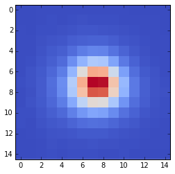
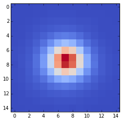
Figure 9: The same source from a stack using SCAMP and SWarp (left) vs a astropyp stack (right). By looking at a single source it is easier to see the improvement made to our PSF by stacking our images by using image coordinates.

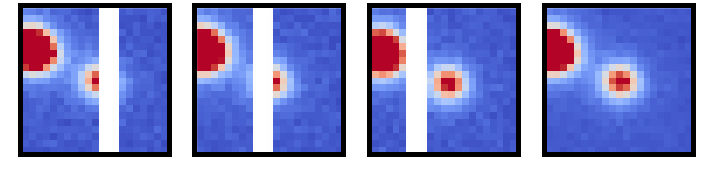
Figure 10: Elimination of bad pixels in the stack. The first three images from the left are single 200s exposures of a source that is bisected by a bleed trail on the CCD. The image on the right is taken from the stacks, which has no bad pixels since none of the images had overlapping data quality masks.

Since the exposures used to create our stacks are only slightly rotated and translated, a linear transformation is sufficient to create the astrometric solution. This is not true later in our pipeline when we compare images from different epochs and need a higher order polynomial to calculate proper motions (see Section A.3.3). Once the solution has been derived the pipeline creates a bivariate spline function to calculate flux as a function of pixel coordinates in the original images. The bivariate spline function is then used to map all of the pixels from the 3 images onto a common coordinate system (slightly larger than the reference image so that all 3 images are contained in their entirety).

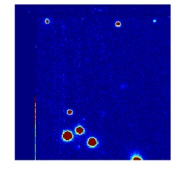
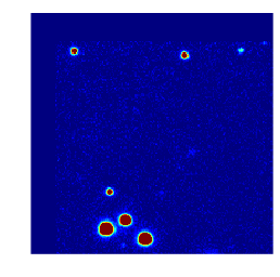
Figure 11: Stacked images using SCAMP and SWarp (top) vs astropyp (bottom). By combining images using image coordinates instead of the less accurate world coordinates (calibrated to GAIA) we are able to significantly improve the quality of our stacked images.

To minimize the effects of bad pixels, the data quality mask derived by the community pipeline is used to mask the image arrays. The mean of each unmasked pixel is used in the stack and any pixels that were masked in all 3 images are masked in the final image and added to a new data quality mask created for the stack. This allows us to save a large number of sources that are partially obstructed by non-overlapping bleed trails in all 3 images (see Figure 10). The final result is an image that has noticeably less noise than the stacks we built using SCAMP and SWarp (see Figures 9 and 11).

When the final GAIA source catalog is released in 2022, the process for reprojecting and stacking our images might be unnecessary, since GAIA aims to have better than 10mas errors (which is better than the errors on DECam image positions). It is even possible that GAIA DR1 may be a large enough improvement to render this procedure unnecessary, or at the very least computationally expensive for a minimal gain in accuracy (our stacks were built before the GAIA DR1 release, so we have yet to test using it to create new stacks). Otherwise this may be the best solution to stack images and calculate proper motions (see Section A.3 for more on calculating proper motions from an astrometric solution).

A.1.1 Windowed Positions

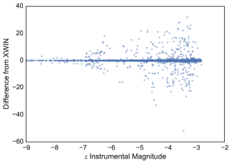
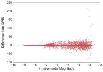
Figure 12: Difference in pixels between the x coordinate detected by SEP and the windowed coordinate XWIN for a single CCD (similar differences are seen with the y and YWIN positions). The shorter (30s) z band exposure has 230 of 2074 sources ($\sim$11%) with a change in position of more than 1" while the longer (200s) i band exposure has 1233 of 4716 sources ($\sim$26%) with a $>$1" coordinate change. Investigation of this effect appears to occur mostly in crowded fields or when a nearby neighbor is not detected by SEP, which is why we see more frequent bad windowed positions in the longer exposures.

Another important feature we added to our code was an improvement to the calculation of windowed positions by SEP/SExtractor (see subsection A.2). SExtractor windowed positions are improved source positions calculated using an iterative procedure to find the weighted average of a sources flux. Usually (for $\gtrsim$95% of detected sources) this is a much more accurate position but as you can see in Figure 12, for a small percentage of sources the windowed position can drift from one point source to a completely different object. Both SExtractor and SEP have flags to mark sources that fail to calculate windowed positions, but in crowded fields we have still observed a small percentage of sources that see their windowed position jump to a nearby brighter source. In order to correct these positions we ignore any windowed positions shifting by more than either an arcsecond or half the distance to the nearest neighbor, whichever is less. Any source whose windowed position is shifted by a larger amount uses its original SExtracted position with a “badwinpos” flag set in the final catalog to note that it has a less accurate position. When calculating the mean position (see Section A.3), observations with bad windowed positions are only used if the same source has a bad windowed position in all of the images in the same epoch, otherwise only the good windowed positions are used to calculate the catalog position.

A.2 Photometry

Source detection and aperture photometry is performed on individual CCDs using the SEP package, a python library derived from SExtractor, one of the fastest codes to detect point sources. The recent SExtractor port to python gives researchers more control over which functions are run, an easier interface to modify parameters, a better understanding of what SExtractor is doing, and more control over the format and contents of the output catalog.

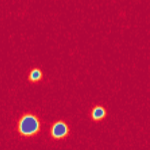
Figure 13: Sample tiles from CCDs S29 (left) and N31 (right) from the same DECam image. The significant distortion in the PSF is obvious to the eye and is the reason we perform PSF photometry on each CCD independently.

Once the sources have been detected the next step is to automatically select PSF stars. Beginning with the source catalog generated by SEP, we remove all sources that have a bad pixel anywhere in their aperture or any other abberation flagged by the DECam community pipeline data quality mask (for our stacks we only flag pixels that were bad in the stack, see Section A.1 for more on the bad pixel mask). To remove crowded stars we reject all sources that have a neighbor within 3 times the detection aperture radius. Although the CCDs near the edge of the DECam focal plane are distorted (See Figure 13), we found that eliminating all sources with a best fit elliptical aperture ratio $>$ 1.5 removes any galaxies or edge effects that may have been missed by the data quality mask without rejecting good data. Finally we eliminate all sources except those with a flux maximum $<$ 100 counts, as DECam is known to be nonlinear in this regime (Bernstein, 2015).

To create the PSF we use a similar procedure to the one implemented in DAOPHOT, loading a normalized subsampled image patch centered on each PSF source. In most cases the exact center of the source is not at the center of the patch, so all of the sources are recentered on the subpixel with the maximum flux, giving a slightly cleaner PSF than a PSF generated using the weighted average position. We then mask all of the pixels outside the circular aperture used for the PSF and store the pixelated PSF array as an astropy Fittable2DModel.

One way to perform PSF photometry is to divide the image into groups (or clusters) of sources, where sources with nearby neighbors are lumped into the same group and PSF photometry is performed on the entire group simultaneously (this is how DAOPHOT works). This can be computationally expensive for very crowded fields, especially in fields where nearly the entire CCD would be treated as a single group (such as in the Galactic plane). It can also lead to instances, if the variance is not accounted for sufficiently, where the brightest sources in a group can dwarf the other sources and ruin the fit for fainter stars.

Instead, we find all of the neighbors for each star that lie within 3 aperture radii ($\sim$10^′′). A patch from the data is extracted, subsampled, and re-centered on the source to be fit, using the same procedure used to generate the PSF. We then simultaneously fit the target source (the one the patch is centered on) as well as it’s neighboring sources (that are only partially contained in the patch). This allows for a much more accurate flux calculation and is also much faster, as fitting an entire group simultaneously often involves fitting a lot of pixels that are not part of one of the sources (although this can be minimized by masking the pixels outside the sources aperture radii). For very crowded images, where nearly all of the sources would be contained in a single group (and thus thousands of sources would need to be simultaneously fit), the group would have to be subdivided into overlapping patches anyway.

Figure 14: Distribution of magnitude errors for all 5+ million sources with observations in multiple bands (top) and $i$ magnitude error as a function of magnitude for the F120 field (bottom). $\sim$78% of $i$ band sources have better than 2% photometry and $\sim$93% have better than 5% photometry (the mean error is $\sim$ 2%). The errors in $zY$ are not quite as good, where both have $\sim$63% of sources better than 2% photometry and 79% better than 5% (with a mean of $\sim$3%).

To calculate the error for each source we look at the residual flux left over by subtracting the PSF model (with the best fit parameters) from the image patch inside the aperture. The error is then the ratio of residual flux to PSF flux, which for the majority of our sources is less than 2%. Figure 14 shows the percentage of sources with PSF error $<$ 2%, $<$5%, and bad sources (with error $>$5%) for the entire SCOCENSUS catalog and for a field calibrated with SDSS. By analyzing results on a select number of CCD images we determined that nearly all the sources with errors $>$5% are either galaxies, sources with high background flux due to very bright distant saturated stars, or unresolved binaries with slightly deformed shapes.

A.3 Calibration

A.3.1 Photometric Calibration

Once the images have been stacked, with instrumental PSF magnitudes calculated, it is still necessary to calibrate the magnitudes to a standard photometric system and calculate their proper motions. One popular way to calibrate DECam photometry is to use a DECam native system, fitting the stellar locus using a code like BIGMACS (Kelly et al., 2014). This method was used by the DES in (Melchior et al., 2015) but requires $g$ band photometry to fit the stellar locus, which we did not take.

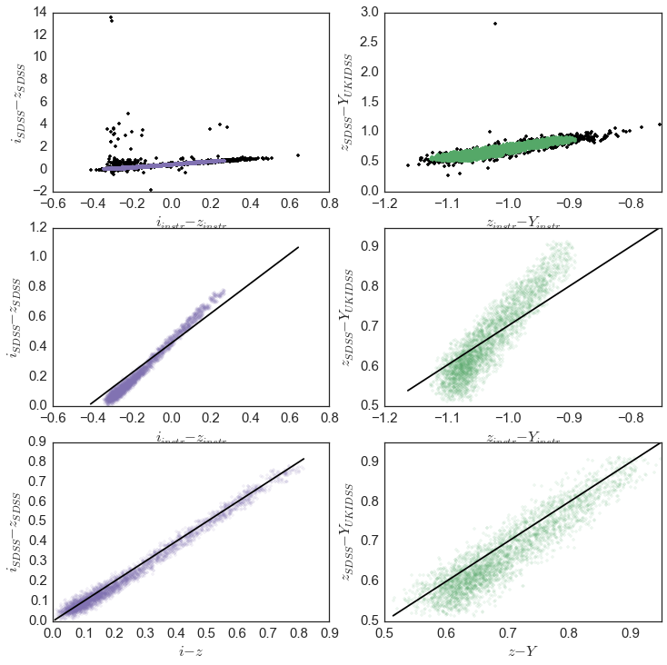
Figure 15: Corrections needed for $i-z$ colors (left column) and $z-Y$ colors (right column) to put DECam instrumental magnitudes on the SDSS AB photometric system (or $z_{SDSS}-Y_{UKIDSS}$ for $z-Y$). The top row shows all of the sources with good psf photometry with outliers removed before fitting the colors are shown in black. The middle row shows the difference between instrumental and SDSS magnitudes with a line with slope unity in black. The last row shows the same relationship after calibration, with a line with slope one in black.

Instead we calibrated our images by taking hourly exposures from standard regions covered by SDSS (for $iz$ bands) and UKIDSS (for $Y$ band). Using the InstCal images we performed PSF photometry on all 3 filters and selected only the isolated, high signal to noise sources (in 3 all bands) to use for calibration. Using astroquery (Ginsburg et al., 2013) we loaded the relevant portions of the SDSS and 2MASS catalogs from Vizier (Ochsenbein et al., 2000) and further restricted our calibration catalog by choosing only sources SDSS flagged as single sources (i.e. no binaries) with good stellar profiles. Unfortunately we neglected to take standard fields in Stripe 82, which is well calibrated and has flagged variable stars and other anomalous sources that could interfere with our calibration. This causes our SDSS fields to have several of sources with unusually large $i-z$ colors that we reject. Once again we used MCMC to remove outliers but found another method that was faster, in this case using the DBSCAN clustering algorithm (Ester et al. 1996; see Figure 15).

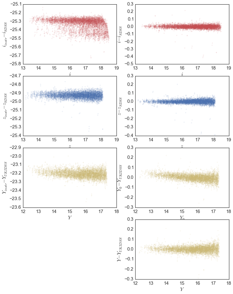
Figure 16: The left column shows the difference between DECam instrumental magnitudes and SDSS (and UKIDSS) magnitudes for matching sources. The right column shows the difference in magnitudes after calibration. In the case of the Y filter we show the difference without the extra magnitude-dependent term and with the magnitude-dependent term (bottom).

While the DECam filters were designed to approximately match the SDSS filters, slight differences in the total throughput and color variations over the FOV make it necessary to add a color correction to the photometric calibration (see Figure 15). To calibrate our colors we use the transformations outlined in Landolt (2007):

$$i_{SDSS}-z_{SDSS} =a+bC_{iz}$$ (3)

$$z_{SDSS}-Y_{UKIDSS} =c+dC_{zY}$$ (4)

where $a,b,c,d$ are coefficients used to make a linear transformation between the reference colors and the instrumental color indices $C_{iz},C_{zY}$ (colors outside the atmosphere), with

$$C_{iz} =i_{instr}-z_{instr}-k_{1}X-k_{2}C_{iz}X$$ (5)

$$C_{zY} =z_{instr}-Y_{instr}-k_{3}X-k_{4}C_{zY}X$$ (6)

where $i_{instr},z_{instr},Y_{instr}$ are the instrumental magnitudes, $k_{x}$ are the extinction coefficients, and $X$ is the airmass.

This allows us to calculate the magnitude of each source in the SDSS system:

$$i =i_{instr}-A_{i}X+Z_{i}+c_{i}(i_{SDSS}-z_{SDSS})$$ (7)

$$z =z_{instr}-A_{z}X+Z_{z}+c_{z}(i_{SDSS}-z_{SDSS})$$ (8)

$$z_{Y} =z_{instr}-A_{zY}X+Z_{zY}+c_{zY}(z_{SDSS}-Y_{UKIDSS})$$ (9)

where $i,z,Y$ are the calibrated magnitudes, $Z_{x}$ are the zero points, $A_{x}$ are the extinction coefficients, $c_{x}$ are the color coefficients, and $y_{0}$ is a magnitude dependent term $\sim$ 1.01 that will be discussed shortly. Since some of the fainter (and redder) sources may be detected in $z$ and $Y$ but not $i$ band images, we calculate a second $z$ magnitude, $z_{Y}$, which has its colors calibrated to the $z-Y$ color as opposed to the more accurate $i-z$. To calculate the coefficients we use all but one of the SDSS fields each night, using the last field as a test set to estimate our photometric errors and verify that we are not overfitting the data. Figure 16 shows the difference between our magnitudes and the SDSS $iz$ magnitudes.

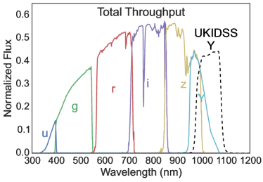
Figure 17: Total system throughput of the various DECam filters (solid lines) and the UKIDSS Y filter (dashed line). Note the extreme difference between DECam Y and UKIDSS Y.

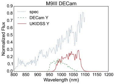
Figure 18: Sample M giant spectra from Pickles (1998). TiO bands and other features detected in UKIDSS Y and not DECam Y are likely the reason that our redder sources seem much fainter in the Y than UKIDSS even after calibration.

The remaining photometric task is to calibrate to UKIDSS $Y$, which is not as straightforward as determining $i$ and $z$. Figure 17 shows the throughput of the DECam filters and the UKIDSS Y filter. Not only is the central wavelength of the two filters different, the shapes of the filters are noticeably different and it is likely that a color calibration is not likely to capture the subtleties of differences in M dwarf spectra like TiO absorption (see Figure 18). If we calibrate Y using similar coefficients to $z_{Y}$ we notice that there appears to be a magnitude dependence in our calibration (possibly due to a blue leak in the Y filter described in Hewett et al. 2006). By modifying the $Y$ equation to

$$Y=M_{0}(Y_{instr}-A_{Y}X)+Z_{Y}+c_{Y}(z_{SDSS}-Y_{UKIDSS})$$ (10)

where $M_{0}\sim 1.01$ is a magnitude dependent term, we see that our calibration is much better but still less accurate than our $iz$ calibration. Properly modeling the difference between the DECam and UKIDSS Y-band throughput might allow us to obtain finer calibrations of our Y-band measurements but is not likely to produce enough of a benefit (for our analysis) to justify spending additional time on it. Figure 19 shows the RMS for all of the CCDs for a single night.

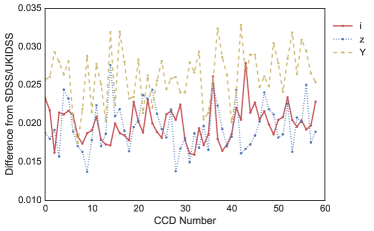
Figure 19: The RMS of the difference between our calibrated photometry and the corresponding magnitudes in SDSS (or UKIDSS for $Y$) for each CCD. Note: this ignores all sources where the difference in magnitude is $>0.1$ mag ($<$1% of the total sources in the field), since our analysis has shown that those are sources that are either variable or have poorly constrained colors in SDSS.

A.3.2 Reddening and Extinction

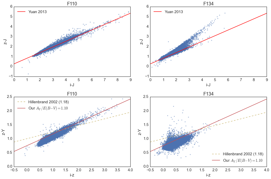
Figure 20: Comparison of reddening vectors calculated from $\frac{A_{i}}{E(B-V)}$, $\frac{A_{z}}{E(B-V)}$ and $\frac{A_{J}}{E(B-V)}$ from Yuan et al. (2013) and $\frac{A_{Y}}{E(B-V)}$ from Hillenbrand et al. (2002) with the reddened $\rho$ Ophiuchus field (F110) and a moderately reddened field in LCC (F134). While the Yuan et al. (2013) values match our observations, $\frac{A_{Y}}{E(B-V)}$ appears to be too high so we use the $\rho$ Ophiuchus field to estimate our $\frac{A_{Y}}{E(B-V)}=1.10$.

To properly estimate effective temperatures (Teff), luminosity functions, and mass functions, we require knowledge of the extinction in $izY$. Yuan et al. (2013) provides estimates for GALEX, SDSS, 2MASS, and WISE passbands, including $A_{i}/E(B-V)=1.71$, $A_{z}/E(B-V)=1.28$, and $A_{J}/E(B-V)=0.72$; while Hillenbrand et al. (2002) estimates $A_{Y}/A_{V}=0.38$ for UKIDSS Y (1.035 $\mu$m). Using our most reddened field, $\rho$ Ophiuchus (F110), and a moderately reddened field in LCC (F134), we measure the reddening vectors $(A_{z}-A_{J})/(A_{i}-A_{J})$ using the extinctions predicted by Yuan et al. (2013) and find good agreement with our observations (see Figure 20). Similarly we measure $(A_{z}-A_{Y})/(A_{i}-A_{z})$, using $A_{V}/E(B-V)=3.1$ from Whittet & van Breda (1980) to convert $A_{Y}/A_{V}$ to $A_{Y}/E(B-V)=1.18$, but find that it is inconsistent with our observations. By fitting the red sources in a $z-Y$ vs $i-z$ color-magnitude diagram (CMD), we estimate $A_{Y}/E(B-V)=1.10$ (see Figure 20).

A.3.3 Astrometric Calibration and Proper Motions

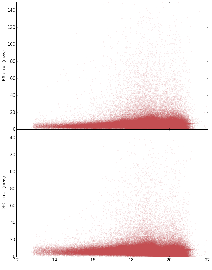
Figure 21: Positional errors in $izY$ in the final SCOCENSUS catalog in the F120 field. For all sources observed in 2015.4 the final position is the average windowed position extracted by SEP from 6 different images: $izY$ stacks and $izY$ short exposures. The errors shown are the RMS values of the measurements used to determine the mean position. For sources only observed in a single image (for example faint sources only detected in $i$ stacks), the mean RMS is used. This is likely to underestimate the errors for sources observed in a single filter but does not affect our analysis as we require $iz$ colors for our candidate selection, meaning all of our sources have a minimum of two measurements for each position.

To calculate mean positions and proper motions we use the same procedure outlined in Section A.1 to reproject exposures of the same field to a common reference frame. This time we combine the short exposures and stacks in all 3 filters for a total of 6 possible exposures of the same source in a given epoch and calculate the average of (x,y) image coordinates in the reference frame of the z-band stacks (which we determined to have the lowest $\chi^{2}$ error when projected onto the GAIA reference frame). This has to be done separately for each CCD and each pointing. We still do not project the $x$ and $y$ positions to a sky catalog yet, as we will reintroduce the >100 mas errors that we have worked carefully to avoid. Instead, for all of the fields observed in both 2013 and 2015, we reproject all of the 2013 image coordinates to the 2015 image coordinates. This allows us to estimate the relative proper motion of each source to within $\sim$10 mas/yr, (20 mas position uncertainties with a two year baseline). We then compare the proper motions we measured with sources in GAIA with proper motion calculations and (after discarding outliers) subtract the mean difference in RA and DEC, yielding an absolute proper motion on the GAIA DR1 reference system. Most likely due to the proximity of our fields to the Galactic plane, less than 10% of our observed sources have proper motions estimates in the GAIA DR1 catalog (Gaia Collaboration et al., 2016).

We also project our 2015 catalog to GAIA DR1 and match each source with observations in the GAIA, UCAC4, 2MASS, USNOB 1.0, and AllWISE catalogs. Although the position errors are much larger than the precision of the DECam image coordinates, sources detected in multiple catalogs with a large enough baseline can yield reasonable proper motions (though still not as accurate as our proper motions with both 2013 and 2015 observations). Figure 21 shows a sample of the internal RMS error for each source as a function of magnitude for the F120 field after calibration. With an RA RMS of 11.0 mas, and DEC RMS of 11.3 mas, the precision of our catalog positions is even better than the $\sim$20 mas precision of the DECam CCDs, with 94.8% of the sources having positional uncertainties less than 20 mas in RA and DEC.

Appendix B Candidate Selection

Our candidate selection is made in several steps of color, magnitude, and proper motion cuts to arrive at well-vetted lists of potential members. The final cuts were chosen iteratively, where our initial photometric cuts influenced our initial proper motion cuts, which allowed us to choose better photometric cuts, etc., until we arrived at a set of conditions that appear to eliminate the bulk of interlopers while discarding as few members as possible. This appendix describes in detail the final procedure used to select our candidates.

B.1 Color-Magnitude Cuts

The first (and most stringent) set of cuts we make is selection based on $i-z$ vs $z$ CMD positions. Figure 22 shows a subset of our survey that covers the $\rho$ Ophiuchus star forming region (to be analyzed in a future paper), where we clearly see substellar sources tracing out an isochrone in $i-z$ vs $z$ color-magnitude space. Unfortunately the UCL and LCC fields investigated in this survey contain a lower density of YLMOs and varying degrees of redenning in a single field of view (even though most of our LCC and UCL objects show $A_{\textrm{v}}<0.1$, background sources can be more strongly reddened). This causes color-magnitude space to become polluted with reddened objects, making it difficult to determine the isochrone for each field and select objects based on photometry alone (see Figure 23).

Figure 22: A subset of field F110 that covers the $\rho$ Ophiuchus star forming complex. We see that in a region with a small age and distance dispersion and nearly isotropic redenning, the members of the complex stand out from older background and foreground sources. The sources shown here are not included in this paper on UCL and LCC but will be analyzed in a future paper.

To make our color cuts we compare our models to the Allard et al. (2011) BT-Settl atmospheric models, using the Asplund et al. (2009) abundances to estimate the effective temperatures (T${}_{\textrm{eff}}$) of our sources. We create a linear interpolation function over the BT-Settl grid for SDSS $iz$, UKIDSS $Y$, and 2MASS $JHK_{s}$ as a function of T${}_{\textrm{eff}}$ and log($g$) (surface gravity). Because the observed magnitudes in the BT-Settl models are given at the stellar surface, they depend on the radius of each stellar/substellar source, which requires a set of isochrones for proper calibration. For this we use the BHAC2015 Baraffe et al. (2015) stellar evolutionary tracks, which allow us to match T${}_{\textrm{eff}}$ and log($g$) from the BHAC2015 isochrones to the BT-Settl atmospheric models. We then use the absolute $M_{J}$ magnitudes from BHAC2015 to calibrate the magnitudes in our BT-Settl grid, which can be converted into observed magnitudes by estimating the distance to our sources. It is regrettable that we require models for our photometric selection because, as was mentioned in the introduction, it is known that these models underestimate the flux for YLMOs at a given age. This means that while the age of UCL and LCC sources are expected to range from $\sim 11-25$ Myr (Pecaut & Mamajek, 2016), our data is better approximated by isochrones from 5-20 Myr. Since the distance to most UCL and LCC sources ranges from $\sim$100-200 pc (Chen et al., 2011), we use the 200 pc at 20 Myr isochrone as the lower magnitude limit for all sources with $i-z<1.7$. We do not have an upper magnitude limit, as sources redder than models predict are still likely to be interesting, and we accept all objects with $i-z\geq 1.7$, since the BHAC2015 models indicate that lower mass sources might become bluer and there are very few background contaminants this red (see Figure 23). After applying these color cuts only $4.7x10^{-2}\%$ of the sources from our full catalog remain as potential members.

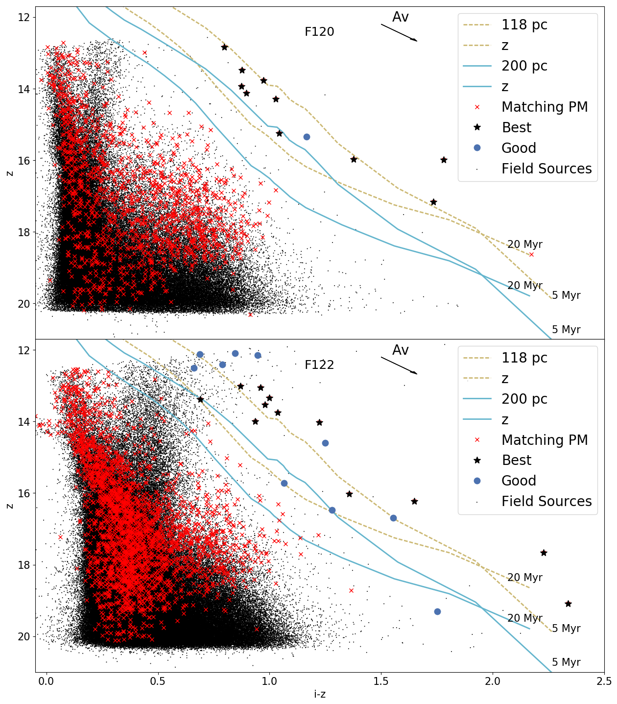
Figure 23: An example of an LCC field with negligible reddening (F120, top, with $b\sim 12.5$) and one 6 degrees closer to the Galactic plane with significant reddening (F122, bottom, $b\sim 6.6$). In F120 there is very little contamination from background sources between the 118 pc isochrones, where only a single object has proper motions consistent with LCC between the 200 pc isochrones. In the more reddened F122 there is a sizable number of interlopers for $z>14$ and 14 objects with similar proper motions between the 200 pc isochrones. These are more likely to be interlopers than actual members and illustrate the necessity to choose a more stringent boundary for our candidates.

B.2 Kinematic Cuts

Kinematic selection is performed by comparing our DECam and Sky proper motions (as defined in Section 2) with the average subgroup velocities predicted by Chen et al. (2011) for UCL and LCC, for all of our sources with errors $\leq 20$ mas/yr, giving us three different levels of cuts. Sources observed in 2013 and 2015 that pass all photometric cuts and have both DECam and Sky proper motions consistent with Sco-Cen are labeled best sources (these necessarily come from the F111, F112, F113, F120, F121, and F122 fields). Sources matching either DECam or Sky proper motions (but not both) are labeled good sources. Sources observed in a single epoch with no previous astrometric measurements, or proper motion errors $>20$ mas/yr, are flagged as having unconstrained proper motions and labeled as “no pm”. The majority of these are faint sources below the detection level in 2MASS, DENIS, AllWISE, and Gaia, so our faintest sources (spectral type L0 and below) only have proper motions in the fields observed in both epochs, but even those can frequently have (relatively) large errors.

Figure 24 shows the fraction of all sources in each image that have proper motions consistent with membership in Sco-Cen and the fraction of all sources in each image that have $iz$ photometry consistent with membership in Sco-Cen. Combining all of the fields together: 4.6% of all objects have Sky proper motions consistent with Sco-Cen, 4.7$\times 10^{-2}$% have $iz$ photometry consistent with Sco-Cen, and for objects observed in 2013 and 2015: 5.6% have DECam proper motions consistent with Sco-Cen and 0.96% have both Sky and DECam proper motions consistent with Sco-Cen.

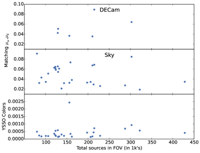
Figure 24: Fraction of all sources in each field with DECam proper motions (top), sky proper motions (middle), and photometry (bottom) consistent with YLMOs in UCL or LCC (depending on the field).

B.3 Photometric Model Fitting

Once we have applied the photometric and kinematic cuts we are left with 1680 candidate objects. Using DECam $izY$ and 2MASS $JHK_{s}$ we can estimate T${}_{\textrm{eff}}$, giving us a spectral class template, by using the BT-Settl and BHAC2015 model grid described in Section B.1. The easiest way to estimate T${}_{\textrm{eff}}$ is to estimate distance, log($g$), age, and A${}_{\textrm{V}}$, and use a least squares-like algorithm to calculate the best fit T${}_{\textrm{eff}}$. This is problematic, as UCL and LCC are known to vary in age from $\sim 11-25$ Myr (Pecaut & Mamajek, 2016) and in distance from $\sim 100-200$ pc (Chen et al., 2011), so using a mean age of 16 Myr and distance of 118 pc for LCC and 142 pc in UCL results in degeneracies that lead to large errors in our T${}_{\textrm{eff}}$ estimates. Using spectral followups on a subset of candidates to be published in a future paper (Moolekamp et al., prep) we compare the spectroscopic spectral types to our predictions obtained by fitting T${}_{\textrm{eff}}$ and find that we can do a much better job estimating spectral types using a Monte Carlo Markov Chain (MCMC).

We use the emcee (Foreman-Mackey et al., 2013) Markov Chain Monte Carlo (MCMC) package to sample the same theoretical grid discussed above and produce estimates of T${}_{\textrm{eff}}$, $\log(g)$, distance, extinction (A${}_{\textrm{V}}$), and mass. In addition to fitting extra parameters, comparing the spectral templates estimated by our MCMC algorithm shows much better agreement with our spectroscopic spectral types, so it is these MCMC derived parameters that we include in our final catalog.

B.4 Removing M Giants

Other than sources with unconstrained proper motions, the largest population of interlopers remaining in our candidate list are M giants which have similar $izY$ colors but very different $JHK_{s}$ colors. Removing these giant stars could have been performed before we fit the candidates to model photometry by assuming A${}_{\textrm{V}}\sim 0.1$ for UCL and LCC, which Pecaut & Mamajek (2016) show is a reasonable estimate. But because A${}_{\textrm{V}}$ is an output of our MCMC algorithm and the values we obtain appear reasonable, we use the estimated A${}_{\textrm{V}}$ for each source and the redenning vectors described in Section A.3.2 to remove all sources more than 0.25 mag from the ($H-K_{s}$,$J-H$) color-color positions predicted by the models. Our giant star cuts are based on the 5 Myr isochrone because there is very little difference in color-color space between the 5 and 10 Myr models and the 5 Myr isochrone contains photometry for lower mass objects, making it easier to eliminate redder giant stars. This is reasonable, as Figure 23 shows that many of our sources lie on or above the 5 Myr isochrone. Once all of our cuts have been applied we are left with a candidate list of mostly M dwarfs, with a large number of fainter objects with unconstrained proper motions that cannot be distinguished based on $izY$ colors alone, leaving us with 562 (163 with proper motions) candidates in LCC and 339 (234 with proper motions) in UCL.

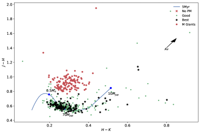
Figure 25: Color-color plot using 2MASS colors to separate M giants from M dwarfs. Sources with $J-H>0.25$ above the 5Myr isochrone are flagged as giants and eliminated. There are also a few sources with very strange $JHK_{s}$ colors ($H-K_{s}$<0 and $H-K_{s}>2$) that are not shown. The source flagged with no proper motion even though it has a 2MASS detection has a very high uncertainty in its proper motions ($>20$ mas) and is consistent with both Sco-Cen and zero proper motion.

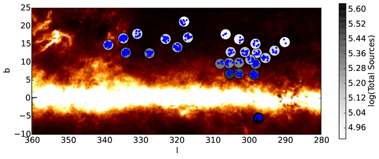
Figure 26: Location of new YLMO’s presented in this paper, in Galactic coordinates, plotted over the SFD dust map (Schlegel et al., 1998). The blue dots are the locations of YLMOs and the large circles are centered at the location of each field of view (not to scale), colored to show the total number of objects in the field. While the total number of sources unsurprisingly increases closer to the Galactic plane, the number of YLMO candidates is more strongly correlated to the number of stellar sources in the field (see Figure 27).

B.5 Estimating Contaminants

We saw in Figure 23 that fields near the Galactic plane can have a substantial number of reddened sources that appear photometrically similar to objects in Sco-Cen and it is necessary to ensure that they aren’t polluting our candidate list. Figure 26 shows that the number of sources in a field increases as it approaches the Galactic center, while the number of candidates in a field does not. This is displayed more quantitatively in Figure 27, where the number of YLMO candidates in a field is shown to be correlated with the number of higher mass stellar candidates in a field (roughly 8:3) and not the fields proximity to the Galactic plane. This gives us a preliminary check that our pipeline is correctly selecting candidates with minimal background contamination.

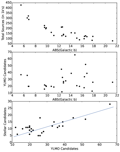
Figure 27: Comparison of the number of sources in a field and it’s proximity to the Galactic plane (top), the number of YLMO candidates and their proximity to the Galactic plane (middle), and the ratio of higher mass stellar candidates/members and YLMO candidates in each field. While the total number of objects in a field increases as it approaches the Galactic plane (top plot), the total number of YLMOs in a field does not (middle plot). Instead there is a much stronger correlation between the number of stellar candidates in a field and the number of YLMO candidates, where a line with $\frac{\textrm{number of YLMOs}}{\textrm{number of high mass stars}}=2.62$ is shown (bottom plot).

We also used spectroscopic follow-up of 17 objects performed using the ARCoIRIS spectrograph last summer to verify both the spectral class of our objects and signatures of low surface gravity that indicate young objects (as opposed to older main-sequence stars or M giants). Of the 17 observed objects, only 1 of them appears to be an older star. These objects were taken from both our “best” and “good” candidate lists, so we estimate that $\sim 5-6$% of our objects are likely to be interlopers. This estimate is also supported by our calculation that 5.6% of our sources have proper motions consistent with Sco-Cen, most of which are coincidental since $<<1\%$ are photometrically consistent (see Section B.2). This is only a rough estimate, as our brighter sources are likely to contain contamination due to reddened stars in the Galactic plane and our fainter substellar sources have larger errors in their proper motions. In the future, creating a model for reddened stars in the Galactic disk will give us a better understanding of the photometric contamination and allow us to provide a more accurate estimate of our background contamination.

References

- Allard et al. (2011) Allard F., Homeier D., Freytag B., 2011, in Johns-Krull C., Browning M. K., West A. A., eds, Astronomical Society of the Pacific Conference Series Vol. 448, 16th Cambridge Workshop on Cool Stars, Stellar Systems, and the Sun. p. 91 (arXiv:1011.5405)
- Allen et al. (2003) Allen P. R., Trilling D. E., Koerner D. W., Reid I. N., 2003, ApJ, 595, 1222
- Ardila et al. (2000) Ardila D., Martín E., Basri G., 2000, AJ, 120, 479
- Asplund et al. (2009) Asplund M., Grevesse N., Sauval A. J., Scott P., 2009, ARA&A, 47, 481
- Astropy Collaboration et al. (2013) Astropy Collaboration et al., 2013, A&A, 558, A33
- Baraffe et al. (2015) Baraffe I., Homeier D., Allard F., Chabrier G., 2015, A&A, 577, A42
- Barrado y Navascués & Martín (2003) Barrado y Navascués D., Martín E. L., 2003, AJ, 126, 2997
- Barrado y Navascués et al. (2007) Barrado y Navascués D., et al., 2007, ApJ, 664, 481
- Bastian et al. (2010) Bastian N., Covey K. R., Meyer M. R., 2010, ARA&A, 48, 339
- Becker et al. (2013) Becker C., Moraux E., Duchêne G., Maschberger T., Lawson W., 2013, A&A, 552, A46
- Bell et al. (2012) Bell C. P. M., Naylor T., Mayne N. J., Jeffries R. D., Littlefair S. P., 2012, MNRAS, 424, 3178
- Bell et al. (2015) Bell C. P. M., Mamajek E. E., Naylor T., 2015, MNRAS, 454, 593
- Bernstein (2015) Bernstein G., 2015, The quirks and qualities of DECam data, http://www.noao.edu/meetings/decam2015/files/GBernstein_DECam_Tucson.pdf
- Bihain et al. (2010) Bihain G., Rebolo R., Zapatero Osorio M. R., Béjar V. J. S., Caballero J. A., 2010, A&A, 519, A93
- Burrows et al. (2001) Burrows A., Hubbard W. B., Lunine J. I., Liebert J., 2001, Reviews of Modern Physics, 73, 719
- Carpenter et al. (2006) Carpenter J. M., Mamajek E. E., Hillenbrand L. A., Meyer M. R., 2006, ApJ, 651, L49
- Chabrier (2003) Chabrier G., 2003, PASP, 115, 763
- Chatterjee et al. (2004) Chatterjee S., Cordes J. M., Vlemmings W. H. T., Arzoumanian Z., Goss W. M., Lazio T. J. W., 2004, ApJ, 604, 339
- Chen et al. (2011) Chen C. H., Mamajek E. E., Bitner M. A., Pecaut M., Su K. Y. L., Weinberger A. J., 2011, ApJ, 738, 122
- Cruz et al. (2009) Cruz K. L., Kirkpatrick J. D., Burgasser A. J., 2009, AJ, 137, 3345
- David et al. (2016) David T. J., Hillenbrand L. A., Cody A. M., Carpenter J. M., Howard A. W., 2016, ApJ, 816, 21
- DePoy et al. (2008) DePoy D. L., et al., 2008, in Ground-based and Airborne Instrumentation for Astronomy II. p. 70140E, doi:10.1117/12.789466
- Dib (2014) Dib S., 2014, MNRAS, 444, 1957
- Epchtein et al. (1997) Epchtein N., et al., 1997, The Messenger, 87, 27
- Espaillat et al. (2012) Espaillat C., et al., 2012, ApJ, 747, 103
- Ester et al. (1996) Ester M., peter Kriegel H., Sander J., Xu X., 1996. AAAI Press, pp 226–231
- Faherty et al. (2013) Faherty J. K., Rice E. L., Cruz K. L., Mamajek E. E., Núñez A., 2013, AJ, 145, 2
- Fazio et al. (2004) Fazio G. G., et al., 2004, ApJS, 154, 10
- Feiden (2016) Feiden G. A., 2016, A&A, 593, A99
- Foreman-Mackey et al. (2013) Foreman-Mackey D., Hogg D. W., Lang D., Goodman J., 2013, PASP, 125, 306
- Gaia Collaboration et al. (2016) Gaia Collaboration et al., 2016, A&A, 595, A2
- Ginsburg et al. (2013) Ginsburg A., et al., 2013, Astroquery v0.1, 10.6084/m9.figshare.805208.v2
- Hernández et al. (2009) Hernández J., Calvet N., Hartmann L., Muzerolle J., Gutermuth R., Stauffer J., 2009, ApJ, 707, 705
- Hewett et al. (2006) Hewett P. C., Warren S. J., Leggett S. K., Hodgkin S. T., 2006, MNRAS, 367, 454
- Hillenbrand et al. (2002) Hillenbrand L. A., Foster J. B., Persson S. E., Matthews K., 2002, PASP, 114, 708
- Hillenbrand et al. (2008) Hillenbrand L. A., Bauermeister A., White R. J., 2008, in van Belle G., ed., Astronomical Society of the Pacific Conference Series Vol. 384, 14th Cambridge Workshop on Cool Stars, Stellar Systems, and the Sun. p. 200 (arXiv:astro-ph/0703642)
- Hogg et al. (2010) Hogg D. W., Bovy J., Lang D., 2010, preprint, (arXiv:1008.4686)
- Hoogerwerf et al. (2001) Hoogerwerf R., de Bruijne J. H. J., de Zeeuw P. T., 2001, A&A, 365, 49
- Jordi et al. (2006) Jordi K., Grebel E. K., Ammon K., 2006, A&A, 460, 339
- Kaiser et al. (1999) Kaiser N., Wilson G., Luppino G., Dahle H., 1999, ArXiv Astrophysics e-prints,
- Kelly et al. (2014) Kelly P. L., et al., 2014, MNRAS, 439, 28
- Kirkpatrick et al. (2008) Kirkpatrick J. D., et al., 2008, ApJ, 689, 1295
- Kraus et al. (2015) Kraus A. L., Cody A. M., Covey K. R., Rizzuto A. C., Mann A. W., Ireland M. J., 2015, ApJ, 807, 3
- Kroupa (2002) Kroupa P., 2002, Science, 295, 82
- Krumholz (2014) Krumholz M. R., 2014, Phys. Rep., 539, 49
- Lada & Lada (2003) Lada C. J., Lada E. A., 2003, ARA&A, 41, 57
- Landolt (2007) Landolt A. U., 2007, in Sterken C., ed., Astronomical Society of the Pacific Conference Series Vol. 364, The Future of Photometric, Spectrophotometric and Polarimetric Standardization. p. 27
- Luhman (2004) Luhman K. L., 2004, ApJ, 616, 1033
- Luhman & Mamajek (2012) Luhman K. L., Mamajek E. E., 2012, ApJ, 758, 31
- Luhman et al. (2000) Luhman K. L., Rieke G. H., Young E. T., Cotera A. S., Chen H., Rieke M. J., Schneider G., Thompson R. I., 2000, ApJ, 540, 1016
- Lyo et al. (2006) Lyo A.-R., Song I., Lawson W. A., Bessell M. S., Zuckerman B., 2006, MNRAS, 368, 1451
- Mamajek et al. (1999) Mamajek E. E., Lawson W. A., Feigelson E. D., 1999, ApJ, 516, L77
- Mamajek et al. (2002) Mamajek E. E., Meyer M. R., Liebert J., 2002, AJ, 124, 1670
- Melchior et al. (2015) Melchior P., et al., 2015, MNRAS, 449, 2219
- Melchior et al. (prep) Melchior P., Moolekamp F., Jerdee M., Armstrong B., Sun A., Bosch J., Lupton R., in prep., scarlet: Source separation in multi-band images by Constrained Matrix Factorization
- Miller & Scalo (1979) Miller G. E., Scalo J. M., 1979, ApJS, 41, 513
- Monet et al. (2003) Monet D. G., et al., 2003, AJ, 125, 984
- Moolekamp et al. (prep) Moolekamp F., Ancietti, Carlos Mamajek E., Luhman K., James D., Metchev S., in prep., ARCoIRIS Observations of New Substellar Objects in the LCC and UCL subgroups of Scorpius-Centaurus
- Murphy et al. (2010) Murphy S. J., Lawson W. A., Bessell M. S., 2010, MNRAS, 406, L50
- Murphy et al. (2017) Murphy S. J., Mamajek E. E., Bell C. P. M., 2017, preprint, (arXiv:1703.04544)
- Ochsenbein et al. (2000) Ochsenbein F., Bauer P., Marcout J., 2000, A&AS, 143, 23
- Pecaut & Mamajek (2016) Pecaut M., Mamajek E., 2016, MNRAS
- Pecaut et al. (2012) Pecaut M. J., Mamajek E. E., Bubar E. J., 2012, ApJ, 746, 154
- Pickles (1998) Pickles A. J., 1998, PASP, 110, 863
- Preibisch & Mamajek (2008) Preibisch T., Mamajek E., 2008, The Nearest OB Association: Scorpius-Centaurus (Sco OB2). p. 235
- Reid & Hawley (2005) Reid I. N., Hawley S. L., 2005, New light on dark stars : red dwarfs, low-mass stars, brown dwarfs, doi:10.1007/3-540-27610-6.
- Reiners (2009) Reiners A., 2009, ApJ, 702, L119
- Rizzuto et al. (2016) Rizzuto A. C., Ireland M. J., Dupuy T. J., Kraus A. L., 2016, ApJ, 817, 164
- Salpeter (1955) Salpeter E. E., 1955, ApJ, 121, 161
- Schlegel et al. (1998) Schlegel D. J., Finkbeiner D. P., Davis M., 1998, ApJ, 500, 525
- Skrutskie et al. (2006) Skrutskie M. F., et al., 2006, AJ, 131, 1163
- Slesnick et al. (2004) Slesnick C. L., Hillenbrand L. A., Carpenter J. M., 2004, ApJ, 610, 1045
- Song et al. (2004) Song I., Zuckerman B., Bessell M. S., 2004, ApJ, 600, 1016
- Sung & Bessell (2010) Sung H., Bessell M. S., 2010, AJ, 140, 2070
- Valdes et al. (2014) Valdes F., Gruendl R., DES Project 2014, in Manset N., Forshay P., eds, Astronomical Society of the Pacific Conference Series Vol. 485, Astronomical Data Analysis Software and Systems XXIII. p. 379
- Whittet & van Breda (1980) Whittet D. C. B., van Breda I. G., 1980, MNRAS, 192, 467
- Wright et al. (2010) Wright E. L., et al., 2010, AJ, 140, 1868
- Yuan et al. (2013) Yuan H. B., Liu X. W., Xiang M. S., 2013, MNRAS, 430, 2188
- Zacharias et al. (2013) Zacharias N., Finch C. T., Girard T. M., Henden A., Bartlett J. L., Monet D. G., Zacharias M. I., 2013, AJ, 145, 44
- de Marchi et al. (2005) de Marchi G., Paresce F., Portegies Zwart S., 2005, in Corbelli E., Palla F., Zinnecker H., eds, Astrophysics and Space Science Library Vol. 327, The Initial Mass Function 50 Years Later. p. 77 (arXiv:astro-ph/0409601)
- de Zeeuw et al. (1999) de Zeeuw P. T., Hoogerwerf R., de Bruijne J. H. J., Brown A. G. A., Blaauw A., 1999, AJ, 117, 354