Box counting dimensions of generalised fractal nests

Abstract

Fractal nests are sets defined as unions of unit $n$-spheres scaled by a sequence of $k^{-\alpha}$ for some $\alpha>0$. In this article we generalise the concept to subsets of such spheres and find the formulas for their box counting dimensions. We introduce some novel classes of parameterised fractal nests and apply these results to compute the dimensions with respect to these parameters. We also show that these dimensions can be seen numerically. These results motivate further research that may explain the unintuitive behaviour of box counting dimensions for nest-type fractals, and in general the class of sets where the box-counting dimension differs from the Hausdorff dimension.

1 Introduction

Research into rectifiability (eg. [Tri93]) has given some unexpected results in the differences between the Hausdorff dimension [Fed69, pg. 171] and the box counting dimension of some countable unions of sets and their smooth generalisations [Tri93, pg. 121-122], such as unrectifiable spirals. Recently, progress has been made in the application of the box counting dimension in the analysis of complex zeta functions, [LRŽ17]. We note especially the discovery of various interesting properties, including a relationship of Lapidus-style zeta functions with the Riemann zeta function and the generalisation of the concept of the box dimension to complex dimensions. Fractal nests, as presented and analysed in [LRŽ17], behave in an unexpected way with respect to the appropriate exponents. There are two general types of behaviour of fractal nests. The well understood type of behaviour of fractal nests concerns sets that locally resemble Cartesian products of fractals [LRŽ17, pg. 227], [ŽŽ05, Remark 6.]. In such sets, the dimension behaves naturally as the sum of the dimensions of “base” sets. What remains less understood are dimensions of fractal nests of centre type. In this case, the dimension is product-like in terms of dimensions of underlying elements, lacking an intuitive geometric interpretation.

This article focuses on a more classical approach to the box-counting dimension, giving examples that may further the understanding of how the box counting dimension behaves with respect to countable unions of similar sets. Whereas in [LRŽ17] and [ŽŽ05] the fractal nests studied are based on $(n-1)$-spheres (hyper-spheres), we study fractal nests $S_{\alpha}$ based on fractal subsets of box counting dimension $\delta$ of such spheres under similar scaling. Our results are compatible with the cited ones, having them as limit cases of full dimension, $\delta=(n-1)$; notably, the dimension are

$$\dim_{B}S_{\alpha}=\frac{\delta+1}{\alpha+1}$$

for the centre type and

$$\dim_{B}S_{\alpha}=\delta+\frac{1}{\alpha+1}$$

for the outer type. The proofs of these results hint at some more general geometric and topological properties.

This paper is divided into five sections. After this introduction we present the main concepts and results of this paper – a dimensional analysis of generalised fractal nests, followed by applications of these results to novel fractal sets with numerical examples. After that, we provide the proofs of our main results and in the final section we remark on some issues and problems that naturally arise from these investigations.

2 Generalised fractal nests

2.1 Box counting dimension

We start with the definition of the box counting dimension as stated in [Fal14, pg. 28] as the alternative definition. By an $\epsilon$-mesh in ${\mathbb{R}}^{n}$ we understand the partition of ${\mathbb{R}}^{n}$ into disjoint (except possibly at the border) $n$-cubes of side $\epsilon$.

Definition 1.

Let $S\subseteq{\mathbb{R}}^{n}$ be a bounded Borel set. By $N_{\epsilon}(S)$ we denote the number of such $n$-cubes of the $\epsilon$-mesh of ${\mathbb{R}}^{n}$ that intersect $S$. We define the upper (lower) box counting dimension of $S$ by

$$\overline{\dim}_{B}S =\inf\left\{\delta\,\Big{|}\,\epsilon^{\delta}N_{\epsilon}(S)\to 0\right\}.$$

$$\bigg{(}\underline{\dim}_{B}S =\sup\left\{\delta\,\Big{|}\,\epsilon^{\delta}N_{\epsilon}(S)\to+\infty\right\}\bigg{)}.$$

Example 1.

The unit $m$-cube $K_{m}=[0,1]^{m}\times\{0\}^{n-m}$ in ${\mathbb{R}}^{n}$ with $m\leq n$ has

$$\overline{\dim}_{B}K_{m}=\underline{\dim}_{B}K_{m}=m$$

because it intersects $\left\lceil\epsilon^{-1}\right\rceil^{m}$ $n$-cubes of side $\epsilon$. Hence, for various $\delta$ we have, as $\epsilon\to 0$,

$$\epsilon^{\delta}\left\lceil\epsilon^{-1}\right\rceil^{m}\to\begin{cases}0,\hbox{ for }\delta>m,\\ 1,\hbox{ for }\delta=m,\\ +\infty,\hbox{ for }\delta<m.\end{cases}$$

The box counting dimension of a set $S$ can be defined in terms of other counting functions, such as the maximum number of disjoint $\epsilon$-balls centred on points of $S$, the minimal number of $\epsilon$-balls needed to cover $S$, similar constructions in equivalent metrics, etc. [Fal14, pg. 30].

One important reformulation of the box counting dimension is the Minkowski-Bouligand dimension. It is formulated in terms of the Lebesgue measure in the ambient space and constructs a natural “contents” function at every dimension, in that regard similar to the Hausdorff dimension and measure.

As $\epsilon$-balls used here and in other literature correspond to the Euclidean metric, we need to compensate for the coefficient for volume of the ball characteristic to this metric and dimension,

$$\gamma_{x}=\frac{\pi^{\frac{x}{2}}}{\Gamma(\frac{x}{2}+1)}.$$

For further discussion of this coefficient and its use in the Minkowski-Bouligand dimension, see [Res13] and [KP99, Chapter 3.3].

Definition 2.

Let $S\subseteq{\mathbb{R}}^{n}$. For $\epsilon>0$, we define the $\epsilon$-Minkowski sausage of $S$ as the set

$$(S)_{\epsilon}=\left\{x\in{\mathbb{R}}^{n}\,|\,d(x,S)\leq\epsilon\right\}.$$

Let $\lambda$ be the Lebesgue measure on ${\mathbb{R}}^{n}$ and denote by $A^{n,d}_{\epsilon}(S)$ the ratio

$$A^{n,\delta}_{\epsilon}(S):=\frac{\lambda(S)_{\epsilon}}{\gamma_{n-\delta}\epsilon^{n-\delta}}.$$

We say that $d$ is the upper (lower) Minkowski-Bouligand dimension of $S$, $\overline{\dim}_{MB}S$ ($\underline{\dim}_{MB}S$) if

$$d =\inf\left\{\delta\,\Big{|}\,\lim_{\epsilon\to 0}A_{\epsilon}^{n,\delta}(S)=+\infty\right\}$$

$$\bigg{(}d =\sup\left\{\delta\,\Big{|}\,\lim_{\epsilon\to 0}A_{\epsilon}^{n,\delta}(S)=0\right\}\bigg{)}.$$

A classical result (eg. [Pes97, Ch. I.2], [Fal14, Prop. 2.4]) is that both upper and lower Minkowski-Bouligand dimensions are exactly equal to the corresponding upper and lower box counting dimensions, so we will only use the box-dimension notation for the discussed dimension.

Definition 3.

For $S\subseteq{\mathbb{R}}^{n}$, if $\underline{\dim}_{B}S=\overline{\dim}_{B}S=d$, we say that $S$ is of box counting dimension $d$, denoting

$$\dim_{B}S=d.$$

For $S$ of box-dimension $d$, we define the normalised upper (lower) Minkowski content of $S$ as

$${\mathcal{M}^{*}_{d}}(S) =\limsup_{\epsilon\to 0}A_{\epsilon}^{n,d}(S),$$

$$\bigg{(}{\mathcal{M}_{*d}}(S) =\liminf_{\epsilon\to 0}A_{\epsilon}^{n,d}(S))\bigg{)}.$$

We say that the set $S\subseteq{\mathbb{R}}^{n}$ of box-dimension $d$ is Minkowski-non-degenerate if ${\mathcal{M}^{*}_{d}}(S)<+\infty$ and ${\mathcal{M}_{*d}}(S)>0$ and denote

$$\dim_{B}S\equiv d.$$

Example 2.

As per the earlier discussion in Example 1, it is easy to show that $K_{m}\subseteq{\mathbb{R}}^{n}$ is of normalised Minkowski content (both upper and lower) equal to $1$ because

$$\frac{\lambda(K_{m})_{\epsilon}}{\epsilon^{n-m}}=\gamma_{n-m}+\sum_{k=0}^{m-1}\gamma_{n-k}\left(\frac{\epsilon}{2}\right)^{m-k}\!E^{(k)}_{m},$$

where $E_{m}^{(k)}$ is the number of $k$-edges of the $m$-cube.

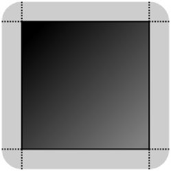
Figure 1: The Minkowski sausage of the unit square in ${\mathbb{R}}^{2}$.

In Figure 1, we have $E_{2}^{(0)}=4$ and $E_{2}^{(1)}=4$ and $\gamma_{0}=1$, $\gamma_{1}=2$ and $\gamma_{2}=\pi$, so we have $\lambda(K_{2})_{\epsilon}=\gamma_{0}+\frac{\epsilon}{2}\gamma_{1}E_{2}^{(1)}+\frac{\epsilon^{2}}{4}\gamma_{2}E_{2}^{(0)}=1+4\epsilon+\pi\epsilon^{2}$.

Example 3.

The set of points $E_{\alpha}=\{k^{-\alpha}\,|\,k\in{\mathbb{N}}\}$ for $\alpha>0$ is of box counting dimension $\frac{1}{1+\alpha}$, with normalised Minkowski contents (both upper and lower) equal to

$${\mathcal{M}_{d}}S=\left(\frac{2}{\alpha\sqrt{\pi}}\right)^{\frac{\alpha}{\alpha+1}}\!(\alpha+1)\,\Gamma\left(\frac{\alpha}{2(\alpha+1)}+1\right).$$

Figure 2: Sets $E_{\alpha}$ of unit normalised Minkowski contents for $\alpha\in\{0.2,0.4,\ldots,5.0\}$.

Figure 2 shows sets $E_{\alpha}$ of unit normalised Minkowski contents in dimensions ranging from $5/6$ at the bottom to $1/6$ in the top row.

2.2 Fractal analysis of $\alpha$-regular generalised fractal nests

Intuitively, an inner $\alpha$-regular fractal nest is the subset of the union of circles of radii $n^{-\alpha}$ where subsets per individual circle are homothetic to each other. The outer $\alpha$-regular fractal nest has radii of form $1-(k+1)^{-\alpha}$.

For a set $S\subseteq{\mathbb{R}}^{n}$ and $x\geq 0$ we denote by $(x)S$ the scaling of the set $S$ by $x$.

Definition 4.

Let $S\subseteq{\mathbb{S}}^{n-1}$ be a Borel subset of the unit sphere in ${\mathbb{R}}^{n}$. We define the $\alpha$-regular fractal nest of centre (outer) type as

$${\mathcal{F}}_{\alpha}S =\bigcup_{k=1}^{\infty}(k^{-\alpha})S$$

$$\bigg{(}{\mathcal{O}}_{\alpha}S =\bigcup_{k=1}^{\infty}(1-k^{-\alpha})S\bigg{)}.$$

Note that

$${\mathcal{F}}_{\alpha}\{1\}=E_{\alpha}$$

and

$${\mathcal{O}}_{\alpha}\{1\}=1-E_{\alpha},$$

where for a set $S$ the expression $1-S$ is defined as $\{1-x\,|\,x\in S\}$, with $E_{\alpha}$ defined in Example 3.

Theorem 1.

Let $S\subseteq{\mathbb{S}}^{n-1}$ be a Borel subset of the unit hyper-sphere in ${\mathbb{R}}^{n}$ such that

$$\dim_{B}S\equiv\delta\geq 0.$$

For every $\alpha>0$ the $\alpha$-regular fractal nest of centre type generated by $S$ has

$$\dim_{B}{\mathcal{F}}_{\alpha}(S)\begin{cases}\equiv\frac{\delta+1}{\alpha+1},\hbox{ for }\alpha\delta<1,\\ =\delta,\hbox{ for }\alpha\delta=1\\ \equiv\delta,\hbox{ for }\alpha\delta>1.\end{cases}$$

Theorem 2.

Let $S\subseteq{\mathbb{S}}^{n-1}$ be a Borel subset of the unit hyper-sphere in ${\mathbb{R}}^{n}$ such that

$$\dim_{B}S\equiv\delta\geq 0.$$

For every $\alpha>0$ that the $\alpha$-regular fractal nest of outer type generated by $S$ has

$$\dim_{B}{\mathcal{O}}_{\alpha}S\equiv\delta+\frac{1}{\alpha+1}.$$

The proofs of both theorems rely on the well-known technique of separating the “core” and the “tail” of the set, the “tail” part consisting of the well-isolated components, and the “core” of the remaining parts.

We take a novel approach to analysing the “core”, where we use the covering lemma (Lemma 5) to replace the components of the core with well-spaced sets without losing the asymptotic and hence dimensional properties, including Minkowski (non)-degeneracy.

3 Application of the generalised nest formulas

In this section, we show some applications of our main results to some known and some novel fractal sets.

3.1 Mapping $m$-cubes to $m$-spheres

Let $K_{m}\subset{\mathbb{R}}^{n}$ be a unit $m$-cube as defined in Example 1 with $m<n$. It is easy to show that for limited domains such as a unit $m$-cube, the mapping

$$\Phi_{n-1}\colon(x_{1},\ldots,x_{n-1})\mapsto( \cos x_{1},\sin x_{1}\cos x_{2},\ldots,$$

$$\sin x_{1}\sin x_{2}\cdots\sin x_{n-1})$$

is bi-Lipschitz.

Thus, any subset of the unit hyper-cube can be mapped to a corresponding set of equal dimension on the hyper-sphere. If we identify $K_{m}$ with its embedding into ${\mathbb{S}}^{n-1}$, applying Theorem 1 we have that

$$\dim_{B}{\mathcal{F}}_{\alpha}K_{m}=\frac{m+1}{\alpha+1}.$$

We note that this formula also applies to $m=0$. Also, for the outer nests, using Theorem 2 we have

$$\dim_{B}{\mathcal{O}}_{\alpha}K_{m}=m+\frac{1}{\alpha+1},$$

again, compatible with $m=0$.

3.2 $(\alpha,\beta)$-bi-fractals

Let $\alpha,\beta>0$. We can identify $E_{\beta}$ with its image on the unit circle of $\Phi_{1}$. Let $D_{\beta}$ be the union

$$D_{\beta}=\Phi_{1}\left(\frac{\pi}{4}(1-E_{\beta})\right)\cup\Phi_{1}\left(\frac{\pi}{4}(1+E_{\beta})\right)\subseteq{\mathbb{S}}^{1}.$$

We have that

$$\dim_{B}D_{\beta}=\frac{1}{1+\beta}.$$

We call the set ${\mathcal{F}}_{\alpha}D_{\beta}$ an $(\alpha,\beta)$-bi-fractal. Its dimension is given by Theorem 1 as

$$\dim_{B}{\mathcal{F}}_{\alpha}D_{\beta}=\frac{\beta+2}{(\beta+1)(\alpha+1)}.$$

(a) $\alpha\approx 0.35$

(b) $\alpha\approx 0.67$

(c) $\alpha\approx 1.00$

(d) $\alpha\approx 1.33$

Figure 3: $(\alpha,\beta)$-bi-fractals of dimension $3/4$

(a) $\dim_{B}{\mathcal{F}}_{\alpha}D_{\beta}\approx 0.25$

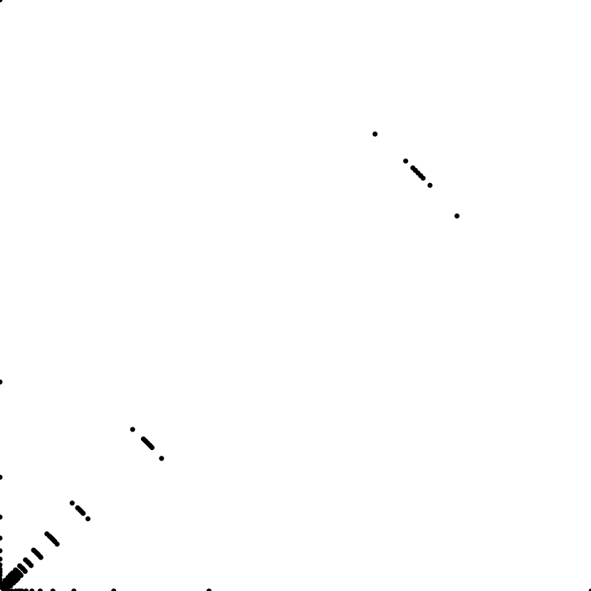
(b) $\dim_{B}{\mathcal{F}}_{\alpha}D_{\beta}\approx 0.5$

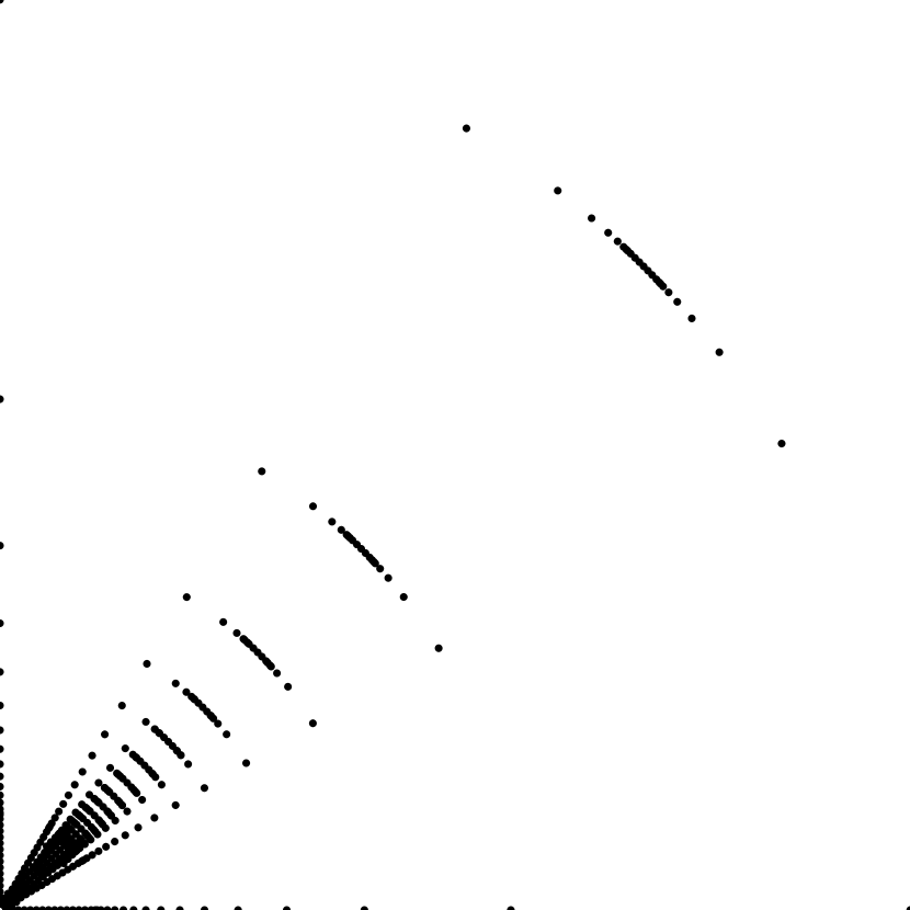
(c) $\dim_{B}{\mathcal{F}}_{\alpha}D_{\beta}\approx 0.75$

(d) $\dim_{B}{\mathcal{F}}_{\alpha}D_{\beta}\approx 1.00$

Figure 4: $(\alpha,\beta)$-bi-fractals of various dimensions.

3.3 Uniform Cantor nests

Intuitively, the uniform Cantor set ${\mathcal{C}}_{N}^{C}$ are Cantor sets “preserving” $N$ copies of themselves totalling $C$ in relative length in each iteration.

In [Fal14, pg. 71] uniform Cantor sets are defined in terms of the number of preserved copies $m$ and the relative gap $r$ (see 5). Modifying that definition to our notation, uniform Cantor sets are defined as follows.

Definition 5 (Uniform Cantor set, [Fal14]).

Let $N\geq 2$ be an integer and $0<r<\frac{1}{N}$. We define the set ${\mathcal{C}}_{n}^{r}$ as the set obtained by the construction in which each basic interval $I$ is replaced by $N$ equally spaced sub-intervals of lengths $r|I|$, the ends of $I$ coinciding with the ends of the extreme sub-intervals. The starting interval for ${\mathcal{C}}_{N}^{r}$ is $[0,1]$.

Figure 5: First four iterations of the uniform Cantor set ${\mathcal{C}}_{3}^{1/4}$.

For the standard Cantor set, ${\mathcal{C}}_{2}^{\frac{1}{3}}$ we have, as is shown in [LP93] and [FC07],

$$\dim_{B}{\mathcal{C}}_{2}^{\frac{1}{3}}\equiv\frac{\log 2}{\log 3},$$

with different upper and lower Minkowski contents,

$${\mathcal{M}^{*}_{d}}{\mathcal{C}}_{2}^{\frac{1}{3}}=\gamma^{-1}_{1-\log_{3}2}4\cdot 2^{-\log_{3}2}\approx 2.27,$$

and

$${\mathcal{M}_{*d}}{\mathcal{C}}_{2}^{\frac{1}{3}}=2\gamma^{-1}_{1-\log_{3}2}\log_{\frac{3}{2}}3\left(\log_{4}\frac{3}{2}\right)^{\log_{3}2}\!\approx 2.19.$$

An older proof of the following proposition can be found in [FC07], where the authors use the simpler formula for (both upper and lower) Minkowski contents omitting the normalising factor.

Proposition 1.

The set ${\mathcal{C}}_{N}^{r}\subseteq{\mathbb{R}}$ is Minkowski non-degenerate with box counting dimension

$$\dim_{B}{\mathcal{C}}_{N}^{r}\equiv-\frac{\log N}{\log r}=d.$$

The upper Minkowski content at the dimension $d$ is

$${\mathcal{M}^{*}_{d}}{\mathcal{C}}_{N}^{r}=2N\left(\frac{s}{2}\right)^{d}\frac{1-r}{1-Nr}\gamma_{1-d}^{-1}$$

and the corresponding lower Minkowski content is

$${\mathcal{M}_{*d}}{\mathcal{C}}_{N}^{r}=\frac{2}{1-d}\left(\frac{1-d}{2d}\right)^{d}\gamma_{1-d}^{-1}.$$

Again, we can use $\Phi_{1}$ to identify ${\mathcal{C}}_{N}^{r}$ with its image on $S^{1}$, and so we have

$$\dim_{B}{\mathcal{F}}_{\alpha}{\mathcal{C}}_{N}^{r}=\frac{1-\log_{r}N}{1+\alpha}$$

and

$$\dim_{B}{\mathcal{O}}_{\alpha}{\mathcal{C}}_{N}^{r}=\frac{1}{1+\alpha}-\log_{r}N.$$

(a) $\alpha\approx 0.33$

(b) $\alpha\approx 0.67$

(c) $\alpha\approx 1.00$

(d) $\alpha\approx 1.33$

Figure 6: ${\mathcal{F}}_{\alpha}{\mathcal{C}}_{3}^{r}$ nests of dimension $3/4$.

(a) $\dim_{B}{\mathcal{F}}_{\alpha}{\mathcal{C}}_{3}^{r}\approx 0.25$

(b) $\dim_{B}{\mathcal{F}}_{\alpha}{\mathcal{C}}_{3}^{r}\approx 0.50$

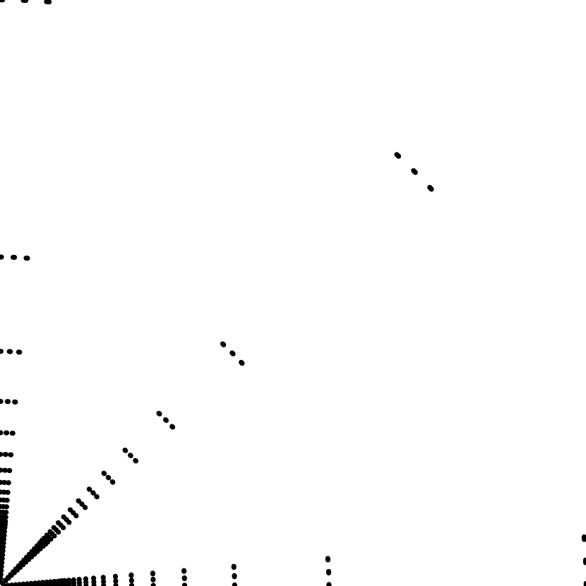
(c) $\dim_{B}{\mathcal{F}}_{\alpha}{\mathcal{C}}_{3}^{r}\approx 0.75$

(d) $\dim_{B}{\mathcal{F}}_{\alpha}{\mathcal{C}}_{3}^{r}\approx 1.00$

Figure 7: ${\mathcal{F}}_{\alpha}{\mathcal{C}}_{3}^{r}$ nests.

3.4 Numerical verification of the results

Since the main results of this article are asymptotic in nature, there is always a risk that we will not be able to reproduce such results in numerical computations. Luckily, as can be seen in figures 8 and 9 we can observe the dimensions to a reasonable accuracy.

We used the same algorithm for producing figures 3, 4, 6 and 7 and also for the explicit computation of the dimensions.

We use the same technique used in the proofs of the main results, in particular we use of Lemma 6 for producing numbers $m_{1}(\epsilon)$ (the number of isolated components, the “tail” of the fractal) and $m_{2}(\epsilon)$, the number of $2\epsilon$-separated elements that cover the “core” of the fractal nest.

For figures 3, 4, 6 and 7 we used a program written in the Python programming language (version 3.6) that outputs an encapsulated PostScript (eps) description of the fractal. PostScript is well-suited as a page description language since it allows for global scaling and setting of line width using the setlinewidth command that is defined in the standard as “up to two pixels” [Ado99, pg. 674] best approximation of the Minkowski sausage of half radius of the given parameter when rendered.

The figures themselves have the half of the line width parameter $\epsilon$ set at $1/300$ of the height and width of the picture.

For $(\alpha,\beta)$-bi-fractals, we first obtain the radius of the element of the nest using $r^{(1)}_{k}=k^{-\alpha}$ for $k\in\{1,\ldots,m_{1}(\epsilon)\}$ and $r^{(2)}_{k}=2k\epsilon$ for $k\in\{1,\ldots,m_{2}(\epsilon)\}$. Then, at each radius $r_{k}^{(i)}$ we draw the the set $D_{\beta}$ by the same construction, using $m_{1}\big{(}\frac{4\epsilon}{\pi r_{k}^{(i)}}\big{)}$ and $m_{2}\big{(}\frac{4\epsilon}{\pi r_{k}^{(i)}}\big{)}$, both with respect to the exponent $-\beta$ instead of $-\alpha$.

For uniform Cantor nests, we repeat the same initial part to obtain $r_{k}^{(i)}$, we use a standard recursive algorithm for describing segments of the Cantor set, where the number of iterations depends on the radius of the nest element, since we are interested only in segments that have gaps larger than $2\epsilon/r_{k}^{(i)}$.

In Figures 3 and 6 we show $(\alpha,\beta)$-bi-fractals ${\mathcal{F}}_{\alpha}D_{\beta}$ and uniform Cantor nests ${\mathcal{F}}_{\alpha}{\mathcal{C}}_{3}^{r}$ of fixed dimension $d=3/4$ and various $\alpha$ with $\beta$ and $r$ computed from

$$r =N^{-\frac{1}{\delta}}$$ (3.1)

$$\beta =\frac{1}{\delta}-1$$ (3.2)

$$\delta =d\alpha+d-1.$$ (3.3)

The constraint of the main result that $\alpha$ plays a role in the total dimension only if $\alpha\delta<1$ limits $\alpha$ to

$$\alpha\in\left\langle{\frac{1}{d}-1,\frac{1}{d}}\right\rangle$$ (3.4)

In Figures 4 and 7 we vary the total dimension $d\in\langle\frac{1}{4},1\rangle$ and we set

$$\alpha=\frac{1}{d}-\frac{1}{2}$$ (3.5)

so that $\alpha$ is always in the centre of the interval given in (3.4). Then we compute $\delta$ using (3.3), and finally we produce the parameters $\beta$ and $r$ from (3.2) and (3.1).

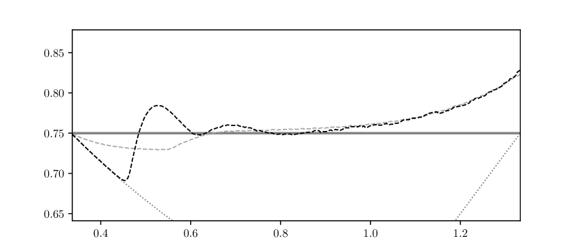
Figure 8: Relative error for numerical computation of the dimensions of ${\mathcal{F}}_{\alpha}D_{\beta}$ (grey dashed line) and ${\mathcal{F}}_{\alpha}{\mathcal{C}}_{3}^{r}$ (black dashed line) for fixed dimension $3/4$ (bold horizontal line).

For Figure 8 we fix the dimension of the whole fractal nest to be $3/4$ and we vary the parameter $\alpha$.

We compute the parameters $\beta$ for the $(\alpha,\beta)$-bi-fractal and $r$ for the ${\mathcal{F}}_{\alpha}{\mathcal{C}}_{3}^{r}$ Cantor nest. For ten different values of $\epsilon$ ranging from $2^{-25}$ to $2^{-10}$ we count the number $N_{\epsilon}$ of points necessary to draw the fractals. Using Python’s scikit-learn library [PVG⁺11], we find the slope for the linear regression of $\ln N_{\epsilon}$ against $-\ln\epsilon$.

As can be seen in Figure 8, the results of these computations come mostly within 10% precision, with relatively short execution time, finishing within minutes on a laptop computer. The falling dotted line at the left side of Figure 8 represents

$$\dim_{B}E_{\alpha}=\frac{1}{\alpha+1}$$

and the rising dotted line on the right side is $\delta$, the dimension of the set copied by the nest. The Cantor nests are sensitive in the beginning, following the $(\alpha+1)^{-1}$ curve. On the right-hand side, as we approach the Minkowski degenerate point when $\alpha=\delta^{-1}$ we should expect the error to grow, as it does.

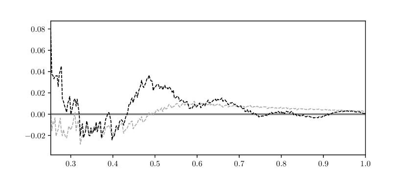
Figure 9: Numerical computation of the dimensions of ${\mathcal{F}}_{\alpha}D_{\beta}$ (grey dashed line) and ${\mathcal{F}}_{\alpha}{\mathcal{C}}_{3}^{r}$ (black dashed line) for varying dimensions.

In Figure 9, we display the relative error of the same method against a varying total box counting dimension, $d\in\left\langle 0.25,1\right\rangle$ as in figures 4 and 7, for $\alpha$ defined by (3.5).

Since $\alpha$ here is defined to be quite distant from $\delta^{-1}$ with

$$\alpha\delta=\frac{1}{2}-\frac{d}{4},$$

we expect the error to be relatively low, with Figure 9 showing the error under 5% for both types of nests.

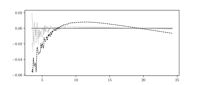
Figure 10: Relative deviations of $\ln N_{\epsilon}$ from linear regression with respect to $-\ln\epsilon$ for $(\alpha,\beta)$-bi-fractals of dimension $3/4$ with $\alpha=4/5$ (dashed grey line), $\alpha=4/3$ (dashed black line) and $\alpha=3$ (dotted grey line).

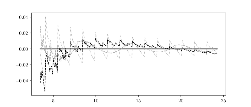
Figure 11: Relative deviations of $\ln N_{\epsilon}$ from linear regression with respect to $-\ln\epsilon$ for uniform Cantor nests of dimension $3/4$ with $\alpha=4/5$ (dashed grey line), $\alpha=4/3$ (dashed black line) and $\alpha=3$ (dotted grey line).

To see the behaviour more clearly, in figures 10 and 11 we show the relative deviations from linear regression for more detailed samples, with 300 samples for $\epsilon$ between $2^{-5}$ and $2^{-35}$. The dimension of the set is fixed at $3/4$.

For $\alpha=4/5$ and $\alpha=3$ in both figures the approximation of the dimension is very good, the numerically obtained dimension is between $0.751$ and $0.754$, while at the critical point (where we lose Minkowski-non-degeneracy, $\alpha=4/3$), the approximate dimension is around $0.82$. At the critical point, the relative error shows the most bias in both figures.

In figure 11 we can also observe the effects of uniform Cantor sets having distinct upper and lower Minkowski content, with visible oscillations of content at different scales.

4 Proofs of main results

In this section we prove the main results. After the introduction of the asymptotic notation we use and the lemmas necessary for the proof of theorems 1 and 2.

4.1 Asymptotic notation

In studying box counting dimensions, asymptotic notation is often useful. Here we opt for $\sim$-style notation, like in [Tri93] for mutually bounded sequences and functions, corresponding to $\Theta$ in classical big-Oh notation [Knu76].

Definition 6 (Sequence and function equivalence).

Let $a_{n}$ and $b_{n}$ be two positive sequences. We say that $a_{k}$ and $b_{k}$ are equivalent and denote it by

$$a_{k}\sim_{k}b_{k}$$

if there exists a number $M\geq 1$ such that for all $k\in{\mathbb{N}}$,

$$M^{-1}a_{k}\leq b_{k}\leq Ma_{k}.$$

Similarly, let $I$ be a set and let $f,g\colon I\to{\mathbb{R}}^{+}$. We say that $f$ and $g$ are equivalent on $I$, denoting

$$f(x)\sim_{x\in I}g(x)$$

if there exists a constant $M\geq 1$ such that for every $x\in I$ we have

$$M^{-1}g(x)\leq f(x)\leq Mg(x).$$

When the domain of equivalence is unambiguous, we will use only the symbol $\sim$ to denote the equivalence.

4.2 The lemmas and the proofs

Lemma 1.

Let $f,g\colon I\to{\mathbb{R}}$ and let $\phi\colon J\times{\mathbb{N}}\to I$ and $m\colon J\to{\mathbb{N}}$. If

$$f(x)\sim_{x\in I}g(x)$$

then

$$\sum_{k=1}^{m(x)}(g\circ\phi)(x,k)\sim_{x\in J}\sum_{k=1}^{m(x)}(h\circ\phi)(x,k).$$

Proof.

Let $x\in J$ and $k\in{\mathbb{N}}$. Since $f\sim_{I}g$ we have

$$M^{-1}(g\circ\phi)(x,k)\leq(f\circ\phi)(x,k)\leq M(g\circ\phi)(x,k).$$

for some $M\geq 1$. Taking the sum of parts of the inequality to $m(x)$, we get

$$M^{-1}\sum_{k=1}^{m(x)}(g\circ\phi)(x,k)\leq{} \sum_{k=1}^{m(x)}(f\circ\phi)(x,k)$$

$$\leq M\sum_{k=1}^{m(x)}(g\circ\phi)(x,k),$$

proving the lemma. ∎

The following Minkowski non-degeneracy condition is a useful intuition on what the box-counting dimension represents, namely that the ambient area of the Minkowski sausage is asymptotically equivalent to radius to the power of the “complementary” dimension of the ambient space.

Lemma 2.

Let $S\subseteq{\mathbb{R}}^{n}$ be such that $\dim_{B}S\equiv d$ and let $L>0$. Then that for $\epsilon\langle 0,L]$ we have

$$\lambda(S)_{\epsilon}\sim\epsilon^{n-d}.$$

Proof.

This is an direct consequence of $A_{\epsilon}^{n,d}$ being bounded from both above and below as $\epsilon\to 0$ and the fact that $\lambda(S)_{\epsilon}$ is continuous and monotonous as a function of $\epsilon$. ∎

Lemma 3.

Let $S\subseteq{\mathbb{R}}^{n}$ be a Borel set and let $x,\epsilon>0$. Then,

$$((x)S)_{\epsilon}=(x)(S)_{\frac{\epsilon}{x}}$$

and, consequently,

$$\lambda((x)S)_{\epsilon}=x^{n}\lambda(S)_{\frac{\epsilon}{x}}.$$

Proof.

Suppose $a\in((x)S)_{\epsilon}$. This is true if and only if

$$\inf_{b\in S}\|a-xb\|\leq\epsilon.$$

Since $x>0$, we get

$$\inf_{b\in S}\left\|{\frac{1}{x}}a-b\right\|\leq\frac{\epsilon}{x},$$

so $a\in((x)S)_{\epsilon}$ if and only if $x^{-1}a\in(S)_{\frac{\epsilon}{x}}$, which is equivalent to $a\in(x)(S)_{\frac{\epsilon}{x}}$, proving the lemma. ∎

Corollary 1.

Under the same assumptions, with $x\geq 1$ ($0<x\leq 1$) we have

$$\lambda(S)_{x\epsilon} \leq x^{n}\lambda(S)_{\epsilon}$$

$$\bigg{(}\lambda(S)_{x\epsilon} \geq x^{n}\lambda(S)_{\epsilon}\bigg{)}.$$

Lemma 4.

Let $S\subseteq{\mathbb{R}}^{n}$ be a Borel set and let $\epsilon>0$. For a sequence $a_{k}\sim_{k}1$,

$$\sum_{k=1}^{m}\lambda(S)_{\epsilon a_{k}}\sim_{m}m\lambda(S)_{\epsilon}.$$

Proof.

Since $M^{-1}\leq a_{k}\leq M$ for some $M\geq 1$, we have that

$$\lambda(S)_{\epsilon a_{k}}\leq\lambda(S)_{\epsilon M}\leq M^{n}\lambda(S)_{\epsilon},$$

and likewise for the lower bound, we have

$$\lambda(S)_{\epsilon a_{k}}\sim_{k}\lambda(S)_{\epsilon}.$$

Taking the sum of both sides from $1$ to $m$, we prove the lemma. ∎

Lemma 5 (Dense covering lemma).

Let $S\subseteq{\mathbb{R}}^{n}$ be a Borel set. Suppose that for every $\epsilon>0$ there is a set $I_{\epsilon}\subseteq{\mathbb{R}}^{+}$ and a (possibly infinite) sequence $a_{k}^{\epsilon}$, such that

$$I_{\epsilon}\subseteq(A^{\epsilon})_{\epsilon}\subseteq(I_{\epsilon})_{\epsilon}.$$

where $m(\epsilon)$ is the (possibly infinite) length of $a_{k}^{(\epsilon)}$ and $A^{\epsilon}=\{a_{k}\,|\,k\leq m(\epsilon)\}$. Then,

$$\lambda\left(\bigcup_{x\in I_{\epsilon}}(x)S\right)_{\epsilon}\sim\lambda\left(\bigcup_{k=0}^{m(\epsilon)}(a_{k}^{(\epsilon)})S\right)_{\epsilon},$$

with respect to $\epsilon$.

Proof.

The inclusions

$$I_{\epsilon}\subseteq(A^{\epsilon})_{\epsilon}\subseteq(I_{\epsilon})_{\epsilon}$$

imply, by triangle inequality,

$$(A^{\epsilon})_{\epsilon}\subseteq(I_{\epsilon})_{\epsilon}\subseteq(A^{\epsilon})_{2\epsilon}.$$

Hence,

$$\left(\bigcup_{x\in I_{\epsilon}}(x)S\right)_{\epsilon}\subseteq\left(\bigcup_{k=0}^{m(\epsilon)}(a_{k}^{(\epsilon)})S\right)_{2\epsilon},$$

and by monotonicity of the Lebesgue measure, and applying Corollary 1 we have

$$\lambda\left(\bigcup_{x\in I_{\epsilon}}(x)S\right)_{\epsilon}\leq 2^{n}\lambda\left(\bigcup_{k=0}^{m(\epsilon)}(a_{k}^{(\epsilon)})S\right)_{\epsilon}$$

By the same argument applied to $(A^{\epsilon})_{\epsilon}\subseteq(I_{\epsilon})_{\epsilon}$, we have

$$\lambda\left(\bigcup_{k=0}^{m(\epsilon)}(a_{k}^{(\epsilon)})S\right)_{\epsilon}\leq 2^{n}\lambda\left(\bigcup_{x\in I_{\epsilon}}(x)S\right)_{\epsilon},$$

proving the lemma. ∎

Lemma 6.

Let $\alpha>0$. For every $\epsilon>0$ there exist numbers $m_{1}(\epsilon)$ and $m_{2}(\epsilon)$ (denoted further by $m_{1}$ and $m_{2}$) satisfying:

$$(m_{1}+1)^{-\alpha}\!\!-(m_{1}+2)^{-\alpha}\! <\!2\epsilon\!\leq m_{1}^{-\alpha}\!\!-(m_{1}+1)^{-\alpha}$$

$$(m_{1}+1)^{-\alpha} \leq 2m_{2}\epsilon\leq m_{1}^{-\alpha}$$

such that

$$m_{1}(\epsilon)\sim m_{2}(\epsilon)\sim\epsilon^{\frac{-1}{1+\alpha}}.$$

Proof.

The existence of $m_{1}$ and the required asymptotic behaviour of $m_{1}$ follows from the fact that

$$n^{-\alpha}-(n+1)^{-\alpha}\sim_{n}n^{-(\alpha+1)}.$$

For $m_{2}$ we observe that $2\epsilon$ fits between $m_{1}^{-\alpha}$ and $(m_{1}+1)^{-\alpha}$, so we can construct

$$m_{2}(\epsilon)=\left\lceil\frac{(m_{1}(\epsilon)+1)^{-\alpha}}{2\epsilon}\right\rceil\leq\frac{(m_{1}+1)^{-\alpha}}{2\epsilon}+1.$$

Suppose $2\epsilon m_{2}>m_{1}^{-\alpha}$. Then

$$m_{1}^{-\alpha} <2\epsilon\left(\frac{(m_{1}+1)^{-\alpha}}{2\epsilon}+1\right)$$

$$=(m_{1}+1)^{-\alpha}+2\epsilon$$

$$\leq m_{1}^{-\alpha}$$

so we have arrived at a contradiction. ∎

Now we turn to the proofs of our main theorems.

Proof of Theorem 1.

Let $\epsilon>0$. We apply Lemma 6 to obtain the functions $m_{1}(\epsilon)$ and $m_{2}(\epsilon)$.

We define the $\epsilon$-tail, ${\mathrm{T}}_{\epsilon}(S)$ as the part of the nest consisting of $\epsilon$-isolated components,

$${\mathrm{T}}_{\epsilon}S=\bigcup_{k=1}^{m_{1}}{\mathrm{(}}k^{-\alpha})S,$$

and we define the $\epsilon$-core, ${\mathrm{C}}_{\epsilon}(S)$ as the remaining components

$${\mathrm{C}}_{\epsilon}S=\bigcup_{k>m_{1}}{\mathrm{(}}k^{-\alpha})S.$$

Now, we have that

$$\lambda\left({\mathcal{F}}_{\alpha}S\right)_{\epsilon}=\lambda\left({\mathrm{T}}_{\epsilon}S\right)_{\epsilon}+\lambda\left({\mathrm{C}}_{\epsilon}S\right)_{\epsilon}.$$

By construction, $2\epsilon m_{2}(\epsilon)$ is an upper bound on the Hausdorff distance of the limit set $\{0\}$ of the whole nest and the $\epsilon$-core.

First, we find the asymptotic behaviour of the core by computing

$$\lambda\left({\mathrm{C}}_{\epsilon}S\right)_{\epsilon}={} \lambda\left(\bigcup_{k>m_{1}}(k^{-\alpha})S\right)_{\epsilon}$$

$$\sim{}\lambda\left(\bigcup_{k=0}^{m_{2}}(2k\epsilon)S\right)_{\epsilon}$$ (4.1)

$$=\sum_{k=0}^{m_{2}}\lambda\left((2k\epsilon)S\right)_{\epsilon}$$

$$=\sum_{k=0}^{m_{2}}(2k\epsilon)^{n}\lambda(S)_{\frac{1}{2k}}$$ (4.2)

$$\sim{} \epsilon^{n}\sum_{k=0}^{m_{2}}k^{n}\cdot k^{\delta-n}\sim{}\epsilon^{n}\sum_{k=0}^{m_{2}}k^{\delta}$$ (4.3)

$$\sim{} \epsilon^{n}m_{2}^{1+\delta}\sim{}\epsilon^{n-\frac{\delta+1}{\alpha+1}},$$

applying Lemma 5 twice at step (4.1), first time to the infinite sequence of $k^{-\alpha}$ for $k>m_{1}$ and then to the finite sequence $2\epsilon k$. At step (4.2) we apply Lemma 3 and to obtain (4.3) we apply Proposition 2 and Lemma 1.

For the tail, we have

$$\lambda\left({\mathrm{T}}_{\epsilon}S\right)_{\epsilon} =\sum_{k=1}^{m_{1}}\lambda\left((k^{-\alpha})S\right)_{\epsilon}$$

$$=\sum_{k=1}^{m_{1}}k^{-n\alpha}\lambda(S)_{k^{\alpha}\epsilon}$$ (4.4)

$$\sim\sum_{k=1}^{m_{1}}k^{-n\alpha}\left(k^{\alpha}\epsilon\right)^{n-\delta}$$

$$\sim\epsilon^{n-\delta}\sum_{k=1}^{m_{1}}k^{-\alpha\delta},$$ (4.5)

where we apply Lemmas 1 and 3 at step (4.4) and Proposition 2 at step (4.5).

Now, if $\alpha\delta<1$, we have

$$\lambda\left({\mathrm{T}}_{\epsilon}S\right)_{\epsilon}\sim\epsilon^{n-\delta}m_{1}^{1-\alpha\delta}\sim\epsilon^{n-\frac{\delta+1}{\alpha+1}},$$

in which case we have

$$\dim_{B}F_{\alpha}(S)\equiv\frac{\delta+1}{\alpha+1}.$$

If $\alpha\delta>1$, we set $\beta=\alpha\delta-1$, and therefore the series $\sum_{k=1}^{\infty}k^{-\alpha\delta}$ converges, so we have

$$\lambda\left({\mathrm{T}}_{\epsilon}S\right)_{\epsilon}\sim\epsilon^{n-\delta},$$

and so the total area is

$$\lambda\left({\mathcal{F}}_{\alpha}S\right)_{\epsilon}\sim\epsilon^{n-\delta}+\epsilon^{n-\frac{\delta+1}{\alpha+1}}=\epsilon^{n-\delta}(1+\epsilon^{\frac{\beta}{\alpha+1}}),$$

proving

$$\dim_{B}F_{\alpha}(S)\equiv\delta.$$

In the case $\alpha\delta=1$ we have

$$\frac{\delta+1}{\alpha+1}=\delta$$

so for the total area we have

$$\lambda\left({\mathcal{F}}_{\alpha}S\right)_{\epsilon}\sim\epsilon^{n-\delta}(1-\ln\epsilon).$$

For any $\zeta>0$ we have

$$\frac{\lambda\left({\mathcal{F}}_{\alpha}S\right)_{\epsilon}}{\epsilon^{n-(\delta+\zeta)}}\sim\epsilon^{\zeta}(1-\ln\epsilon)\to 0$$

for the upper dimension and

$$\frac{\lambda\left({\mathcal{F}}_{\alpha}S\right)_{\epsilon}}{\epsilon^{n-(\delta-\zeta)}}\sim\epsilon^{-\zeta}(1-\ln\epsilon)\to+\infty,$$

for the lower dimension, proving

$$\dim_{B}F_{\frac{1}{\delta}}S=\delta,$$

a Minkowski-degenerate case. ∎

Proof of Theorem 2.

Let $\epsilon>0$. Again, we introduce $m_{1}$ and $m_{2}$ using Lemma 6. Also, as in the previous proof, we define the $\epsilon$-tail and $\epsilon$-core; the $\epsilon$-tail, ${\mathrm{T}}_{\epsilon}S$ as the part of the nest consisting of $\epsilon$-isolated components, and the $\epsilon$-core, ${\mathrm{C}}_{\epsilon}(S)$ as the remaining components.

Now, we have that

$$\lambda\left({\mathcal{O}}_{\alpha}S\right)_{\epsilon}=\lambda\left({\mathrm{T}}_{\epsilon}S\right)_{\epsilon}+\lambda\left({\mathrm{C}}_{\epsilon}S\right)_{\epsilon}.$$

For the tail, we compute

$$\lambda\left({\mathrm{T}}_{\epsilon}S\right)_{\epsilon} =\sum_{k=1}^{m_{1}}\lambda\left((1-k^{-\alpha})S\right)_{\epsilon}$$ (4.6)

$$=\sum_{k=1}^{m_{1}}\left(1-k^{-\alpha}\right)^{n}\lambda(S)_{\epsilon(1-k^{-\alpha})^{-1}}$$ (4.7)

$$\sim m_{1}\lambda(S)_{\epsilon}\sim\epsilon^{n-\delta-\frac{1}{\alpha+1}},$$ (4.8)

applying Lemma 3 at step (4.6) and Lemmas 1 and 4 at step (4.7).

For the core, we have

$$\lambda\left({\mathrm{C}}_{\epsilon}S\right)_{\epsilon}={} \lambda\left(\bigcup_{k>m_{1}}(1-k^{-\alpha})S\right)_{\epsilon}$$ (4.9)

$$\sim{} \lambda\left(\bigcup_{k=0}^{m_{2}}{(1-2k\epsilon})S\right)_{\epsilon}$$ (4.10)

$$=\sum_{k=0}^{m_{2}}(1-2k\epsilon)^{n}\lambda(S)_{\frac{\epsilon}{1-2k\epsilon}}$$ (4.11)

$$\sim{} m_{2}\lambda(S)_{\epsilon}\sim\epsilon^{n-\delta-\frac{1}{\alpha+1}},$$ (4.12)

by applying Lemma 5 at step (4.9), Lemma 3 at step (4.10). To apply Lemma 4 at step (4.11) we note that

$$1-m_{1}^{-\alpha}<1-2k\epsilon\leq 1$$

from the defining condition on $m_{2}$ (Lemma 6) on $m_{2}$. At step (4.12) we also apply Lemma 1.

Thus, we have shown that

$$\dim_{B}{\mathcal{O}}_{\alpha}S\equiv\delta+\frac{1}{\alpha+1}.$$

∎

5 Closing remarks and open problems

In this article we have shown that an $\alpha$-regular fractal nests based on a set $S$ of non-degenerate box counting dimension $\delta$, has dimensions

$$\dim_{B}({\mathcal{F}}_{\alpha}S)=\frac{\delta+1}{\alpha+1}\hbox{ or }\dim_{B}({\mathcal{F}}_{\alpha}S)=\delta$$

for nests of centre type, with $\alpha\delta<1$ for the first case and $\alpha\delta\geq 1$ for the second, and we have shown

$$\dim_{B}({\mathcal{O}}_{\alpha}S)=\delta+\frac{1}{\alpha+1}$$

for the outer type.

These results concur with examples given in [LRŽ17] for hyper-spheres ${\mathbb{S}}^{n-1}\subseteq{\mathbb{R}}^{n}$, where

$$\dim_{B}{\mathcal{F}}_{\alpha}{\mathbb{S}}^{n-1} =\max\left\{n-1,\frac{n}{\alpha+1}\right\},$$

$$\dim_{B}{\mathcal{O}}_{\alpha}{\mathbb{S}}^{n-1} =n-\frac{\alpha}{\alpha+1}.$$

We have also shown that for sets ${\mathcal{F}}_{\alpha}S_{\delta}$ of dimension $d$ based on Minkowski non-degenerate sets $S_{\delta}$ of dimension $\delta$ we have the following relations:

$$\alpha \in\left\langle{\frac{1}{d}-1,\frac{1}{d}}\right\rangle,$$

$$\delta =d\alpha+d-1.$$

These relationships allow us to study the efficacy of simpler numerical techniques for fractal sets presented in this article.

It is well known [Fal14, Fed69, Tri93] that the box counting dimension is not continuous with respect to countable unions. The exact behaviour in examples given here points to a subtler structure that explains the formulas for fractal nests.

For the outer type of nests, this has already been discussed in [ŽŽ05, Remark 6], but the behaviour of centre-type nests remains less well understood. The formula for the centre-type nests obtained here points to a multiplicative operation on the dimensions. Such behaviour of dimensions is well known mostly in vector spaces for tensor products. We propose here that there exists an abstract tensor-like product $\otimes$ on Borel sets such that

$${\mathcal{F}}_{\alpha}S\approx(S\times I)\otimes{\mathcal{F}}_{\alpha}\{1\}$$

with $\approx$ guaranteeing the existence of a bi-Lipschitz map between the sets. We expect the following to hold,

$$\dim_{B}(A\otimes B)=\dim_{B}A\cdot\dim_{B}B,$$

along with $\otimes$ being distributive with respect to Cartesian products (which behave additively).

Perhaps such a product could be found through an analogy between Lipschitz (or bi-Lipschitz) maps that don’t increase or preserve the box dimension, respectively, in uniform spaces [Bou91, Chapter 2] and linear maps in vector spaces, possibly using a kind of a smash product [Bre93, pg. 435].

References

- [Ado99] Adobe Systems Incorporated. PostScript language reference, third edition. Addison-Wesley, 1999.
- [Bou91] Nicolas Bourbaki. General topology. Chapters 1–4. Springer-Verlag, Heidelberg, 1991.
- [Bre93] Glen E Bredon. Topology and Geometry (Graduate Texts in Mathematics). Springer-Verlag, New York, 1993.
- [Fal14] Kenneth Falconer. Fractal Geometry: Mathematical Foundations and Applications, 3rd Edition. Wiley, Feb 2014.
- [FC07] Jiang Feng and Shirong Chen. The Minkowski content of uniform Cantor set. Acta Mathematica Scientia, 27(4):641–647, 2007.
- [Fed69] Herbert Federer. Geometric Measure Theory, volume 153 of Grundlehren der mathematischen Wissenschaften. Springer-Verlag, Berlin, 1969.
- [Knu76] Donald E Knuth. Big omicron and big omega and big theta. ACM Sigact News, 8(2):18–24, 1976.
- [KP99] Steven G. Krantz and Harold R. Parks. The Geometry of domains in space. Birkh’:auser, Boston, 1999.
- [LP93] Michel L Lapidus and Carl Pomerance. The Riemann zeta-function and the one-dimensional Weyl-Berry conjecture for fractal drums. Proceedings of the London Mathematical Society, 3(1):41–69, 1993.
- [LRŽ17] Michel L Lapidus, Goran Radunović, and Darko Žubrinić. Fractal zeta functions and fractal drums: higher-dimensional theory of complex dimensions. Springer, 2017.
- [Pes97] Yakov B Pesin. Dimension theory in dynamical systems: contemporary views and applications. University of Chicago Press, 1997.
- [PVG+11] F. Pedregosa, G. Varoquaux, A. Gramfort, V. Michel, B. Thirion, O. Grisel, M. Blondel, P. Prettenhofer, R. Weiss, V. Dubourg, J. Vanderplas, A. Passos, D. Cournapeau, M. Brucher, M. Perrot, and E. Duchesnay. Scikit-learn: Machine learning in Python. Journal of Machine Learning Research, 12:2825–2830, 2011.
- [Res13] Maja Resman. Invariance of the normalized Minkowski content with respect to the ambient space. Chaos, Solitons & Fractals, 57:123–128, 2013.
- [Tri93] Claude Tricot. Curves and fractal dimension. Springer-Verlag, New York, 1993.
- [ŽŽ05] Darko Žubrinić and Vesna Županović. Fractal analysis of spiral trajectories of some planar vector fields. Bulletin des Sciences Mathématiques, 129(6):457–485, 2005.