Hierarchical evolutive systems, fuzzy categories and the living single cell

Abstract

In this article, the theory of hierarchical evolutive systems of Ehresmann and Vandremeersch [Bull. Math. Bio. 49, 13-50 (1987)] is improved by considering the categories of the theory as fuzzy sets whose elements are the composite objects formed by the arrows and corresponding vertices of their embedded graphs. This way each category can be represented as a point in the states space $\left[0,1\right]^{N}$ $\subset$ $\mathbb{R}^{N}$. The introduction of a diffeomorphism, that acts in this context as a functor between categories, allows to define a measure preserving dynamical system. In particular, we apply this formalism to describe a living single cell. We propose for its state at a given time a hirerchical category with three levels (molecular, coarse-grained and cellular levels) related by adequate colimits. Each level involves the main functional and structural modules in which the cell can be partitioned. The time evolution of the cell is drived by a transformation which is a $N$-dimensional generalization of the Ricker map whose parameters we propose to be determined by requiring that, as hallmark of its behavior, the living cell to evolve at the edge of chaos. From the dynamical point of view this property manifests in the fact that the largest Lyapunov exponent is equal to zero. Since in a rather complete model of the living cell the huge number of involved parameters can make of the calculations a hard task, we also propose a toy model, with fewer parameters to be determined, which emphasizes the cellular fission.

1 Introduction

The efforts made to theoretically describe complex systems have a long history with a broad spectrum of results depending of the involved complexity[1]. In the most successful extreme we have the statistical physics of systems of many identical particles interacting among them via relatively simple forces[2, 3]. But, even for many physical systems, the difficulty of the problems is sometimes far beyond the applicability of statistical physics methods. In disciplines such as economics, social sciences and very particularly biological sciences, the troubles are generally worse being the possibility of applying accurate mathematical techniques almost null in most of the cases.

Perhaps the non physical areas in which there have been major advances in this sense are in the computer sciences. At this respect we must call the attention on the particular relationship between the dynamical systems theory and aspects of computation such as the computational capability in cellular autonoma[4, 5]. Of course, the Boltzmann´s dynamical foundation of statistical mechanics[2, 6] has already been showing us, for a long time now, the potentiality of the theory of dynamical systems to study complex systems.

In typical systems describing social or biological phenomena, we have diverse kinds of elements with their own properties and functions as well as the corresponding interactions among them. The elements number is not large enough as to apply the law of large numbers to them, so the statistical tools are in general not useful for studying these systems.

A convenient way to account for biological systems, within the philosophy of the general systems theory[7], is given by graphs, where the vertices are the diverse elements of the system and the arrows linking them the functional relations among these elements. This is the point of view taken by the Chicago school[8] in its relational theory of biological systems[9, 10]. The approach appeals to the categories theory[11] as the main mathematical tool. However the initial works in this direction consider just the basic notions of categories as well as their simplest constructions.

Subsequent work focused on the response to central questions about complex systems: the binding problem, the emergence problem and the hierarchy problem. A.C. Ehresmann  and J-P.Vandremeersch attempted to give answer to these and other fundamentals problems of complex systems in their theory of hierarchical evolutive systems[12, 13]. In this theory the state of the system under study at a given time is represented by a hierarchical category and its evolution along the time by a sequence of such categories. The passage from the state at a given time to another state in the sequence being governed by a functor. Each functor is determined by a list of objectives that transform the considered category into the new state by adding new elements, or eliminating others, or bounding previously unbound patterns and colimits, etc. These operations are mainly descriptive, a quantitative formulation of them being, in general, a very hard task. Thus, the application of the modern theory of dynamical systems in order to follow the evolution in time of complex systems, particularly biological systems, which are described using the hierarchical evolutive theory is not as direct as would be desirable.

In this article we try to close this gap by introducing the concept of fuzzy categories in the theory of Ehresmann  and Vandremeersch[13]. This way the states space X can be seen as the subset $\left[0,1\right]^{N}$ of  $\mathbb{R}^{N}$ ($\mathbb{R}=$ set of real numbers, $N=$ dimension of X), each point of X being a fuzzy category. Moreover we can define a smooth dynamical system where the dynamics are given by adequate diffeomorphisms so that all the concepts and techniques of the modern theory of dynamical systems can be applied. Thus, it will be possible to determine several quantities, such as the Lyapunov exponents, that will give us rich information about the systems dynamical behavior[14]. It is worth noticing that the abstract theory of dynamical systems in the context of categories has been already considered by diverse authors but, within a pure theoretic spirit, as a tool to relate different mathematical fields and concepts[15, 16].

In particular, in this work we focus into the application of the proposed formalism to describe some aspects of the living single cell. The theoretical study of the living single cell (specifically a minimal isolated bacterium) has deserved increasing attention in the last forty years. The efforts have mainly pointed out towards the development of models and mathematical methods that facilitate the computer simulation of one such a synthetic cell[17]. We can mention in this context the coarse-grained Cornell Escherichia coli B/r-A model[18]. In models posed at a coarse-grained level some finer details of interest can be incorporated in specific modules, so we can talk of hybrid models[19].

The idea of modular biology[20] is what predominates in the route towards the simulation of a whole-cell. The modules represent different types of processes inside the cell and each one is handled with an accurate mathematical tool. The integration of all the modules within a common framework is then essential in order to simulate the whole-cell behavior[21]. The results in this direction are very promising[22, 23].

In our fuzzy hierarchical categories approach we can contemplate different degrees of detail: from finer molecular patterns to coarse-grained patterns to patterns involving global cellular objects and functions. This is naturally accounted by colimit binding processes. Actually our strategy is in some sense the inverse one of that considered by bioinformaticians in their whole-cell simulations. Whereas they, in a modular approach, resort as much as it is possible to finer levels, we use the finer levels just to determine, by means of colimits, objects and relations at higher levels and try to describe their dynamics (reductionism vs. emergence[24]).

A crucial point in the dynamical description of the living cell using our fuzzy hierarchical categories is the assignation of the dynamics, say the diffeomorphisms that transform with time categories into categories. In principle the functional form of these maps, that account for the cell cycle, is unknown for us. To solve this difficulty we propose a high-dimensional generalization of the Ricker map[25] with its parameters determined by requiring that the resulting system dynamical behavior verifies fundamental issues. In the first place of the requirements we consider the putative fact that life develops at the edge of chaos[26, 27, 28], a regime that, from the point of view of the theory of dynamical systems, extends in between the ordered phase defined by period-2ⁿcycles and the unpredictable chaos. It is known that this behavior manifests as that the largest Lypunov exponent is zero. This should mean that the sensitivity to initial conditions as well other system dynamical properties, such as the rate of entropy increase, asymptotically follow a power law instead of an exponential one[29, 30, 31]. We additionally demand that the composition law between the category fuzzy elements be verified.

The paper is organized as follows. In the next section we introduce the fuzzy hierarchical categories. First we review the basic concepts of categories in general and hierarchical categories in particular as considered by Ehresmann  and Vandremeersch[12, 13]. Then the main definitions and properties of fuzzy sets as given by Zadeh[32] are shown for, finally, put both, the hierarchical categories and the fuzzy sets, together in order to define the fuzzy hierarchical categories, the main objects in our description. Section III is devoted to remember the principal concepts and definitions regarding the general theory of dynamical systems. The notion of maximum Lyapunov exponent is reviewed since it will be an important tool in our work. We also discuss the application, in general, of these ideas to probability spaces whose elements are the fuzzy hierarchical categories that we have introduced before. The dynamical theory for fuzzy hierarchical categories developed in previous Sections is used in Section IV to describe, in particular, the living single cell. We present a hierachical scheme for the category that represent the state of a single cell at a given time as a coarse-grained level pattern whose elements are colimits of patterns at a finer level. These patterns represents the main modules in which we consider the cell can be partitioned: mater and energy generation (metabolism), information storage (DNA), information translation (RNA) and information realization (proteins). In turn, the colimit of the coarse-grained pattern gives at the higher hierarchical level the single functional cell. We consider in our hierarchical model the possibility of binary fission. The diagram also help us to propose the parametrized map that transforms the categories with time and we discuss the parameters determination in order that the system evolves at the on-set of the chaos. In this Section we also consider a simplification of the original diagram that make easier the calculations. This diagram can be taken as a toy model of the real single cell.

2 Fuzzy hierarchical categories

This Section is devoted to introduce the main objects in our description of complex systems: the fuzzy hierarchical categories.

2.1 Categories

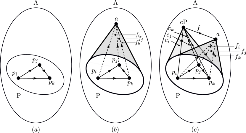
Figure 1: a) Pattern P in the category A; b) Collective link $\left(f_{i}\right)_{i\in\mathbf{I}}$ ($\mathbf{I=}\left\{i,j,k\right\}$) from the pattern P to the object $a$ in the category A; c) Colimit cP of the pattern P in the category A. The collective link from P to cP is $\left(c_{i}\right)_{i\in\mathbf{I}}$ ($\mathbf{I=}\left\{i,j,k\right\}$). We also show the collective link $\left(f_{i}\right)_{i\in\mathbf{I}}$ ($\mathbf{I=}\left\{i,j,k\right\}$) from the pattern P to the object a in the category A that binds into the unique link $f:$cP$\rightarrow$a such that $f_{i}=f\cdot c_{i}$ for each $i\in\mathbf{I}$.

We start considering categories in general. Following very close the work by Ehresmann  and Vandremeersch[13], we give a few definitions to introduce the subject.

Definition 1: A directed graph $G$ is a set of objects (vertices) and a set of arrows (directed edges) from a vertex $a$ to a vertex $b$, denoted by $f:a\rightarrow b$. Here $a$ is the source of the arrow $f$ and $b$ its target.

Definition 2:  A category $\mathbf{A}$ is a pair constituted of a graph and an internal law of composition on the graph. The law associates to successive arrows $f:a\rightarrow b$ and $g:b\rightarrow c$ a third ar$\operatorname{row}$ of the graph $h=g\cdot f:a\rightarrow c$ so that the following properties are verified:

i) Associativity. Given  $f:a\rightarrow b$, $g:b\rightarrow c$ and $h:c\rightarrow d$, the composites $\left(h\cdot g\right)\cdot f:a\rightarrow d$ and $h\cdot\left(g\cdot f\right):$ $a\rightarrow d$ are equal so we can unambiguously write $h\cdot g\cdot f:$ $a\rightarrow d$.

ii) Identity. For each vertex $a$ in the graph there is a closed arrow $i_{a}:a\rightarrow a$ called the identity of $a$. The identity is such that for any other arrow $f:a\rightarrow a$ is $f\cdot i_{a}:a\rightarrow a=$ $i_{a}\cdot f:a\rightarrow a$ $=f:a\rightarrow a$.

Definition 3: A pattern P in the category $\mathbf{A}$ (Fig. 1a) is a family $\left(p_{i}\right)_{i\in\mathbf{I}}$ of objects of $\mathbf{A}$ indexed by a finite set of indices $\mathbf{I}$. The objects $p_{i}$ are the components of the pattern and are such that, for each each pair of indices $\left(i\text{, }j\right)$ there is a set of links from $p_{i}$ to $p_{j}$ called the distinguished links.

Definition 4: Let P be a pattern in the category $\mathbf{A}$. A collective link from P towards an object $a$ of $\mathbf{A}$ (Fig.1b) is a family $\left(f_{i}\right)_{i\in\mathbf{I}}$ of individual links of $\mathbf{A}$ such that associated to each index $i$ of the pattern is a link $f_{i}$ from the component $p_{i}$ to $a$.

Definition 5: An object of a category $\mathbf{A}$ is called the colimit of a pattern P in $\mathbf{A}$ (denoted cP) (see Fig. 1c) if the following two conditions are satisfied:

i) there exists a collective link $\left(c_{i}\right)_{i\in\mathbf{I}}$ called the collective binding link ($c_{i}$ is the binding link from $p_{i}$ to cP );

ii) each collective link $\left(f_{i}\right)_{i\in\mathbf{I}}$ from the pattern P to any object $a$ of $\mathbf{A}$ binds into one and only one link $f$ from cP to $a$ which verifies the relations

$$f_{i}=f\cdot c_{i}\text{ for each index }i\in\mathbf{I}.$$

2.2 Hierarchical categories

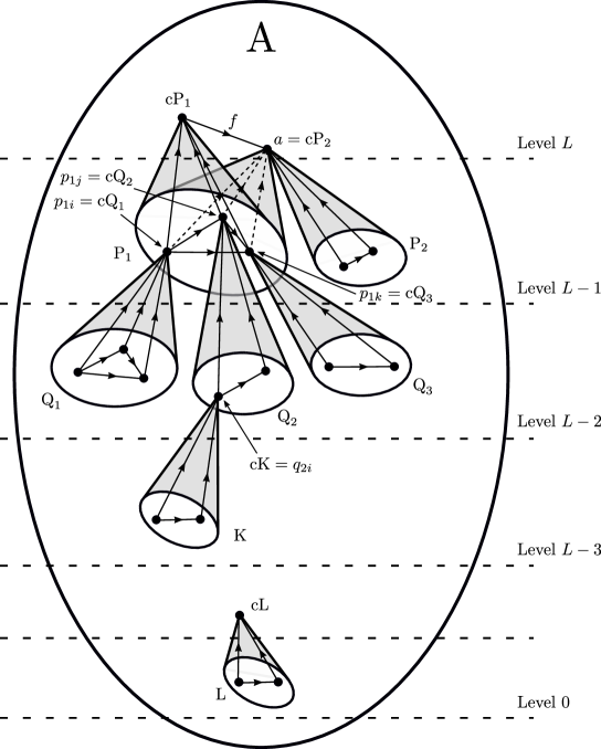
Figure 2: Hierarchical category.

Definition 6: A hierarchical category is a category $\mathbf{A}_{h}$ whose objects are partitioned into a finite sequence of levels $0,1,\cdots,L$ , in such a way that any object $a$ of the level $\ell+1$ is the colimit in $\mathbf{A}_{h}$ of at least one pattern P included in levels lower than $\ell+1$ (Fig. 2).

The previous definitions guarantee that the relations among the components at a given level are coherent with the relations among components at lower levels.

2.3 Fuzzy sets

2.3.1 Definition

We give a definition of fuzzy sets and some of their main properties[32].

Definition 7: Let $X$ be a collection of objects. We define a fuzzy set $\tilde{A}$ as a set of pairs:

$$\tilde{A}=\left\{\left(x,\mathbf{\chi}_{A}(x)\right)\text{: }x\in X\text{, }\mathbf{\chi}_{A}:X\rightarrow\left[0,1\right]\right\}.$$ (1)

The function $\mathbf{\chi}_{A}:X\rightarrow\left[0,1\right]$ is the membership (characteristic) function for the elements of $X$ in $A$.

2.3.2 Properties

a) Equality

$$\left(\tilde{A}=\tilde{B}\right)\Longleftrightarrow\forall x:x\in X\Longrightarrow\mathbf{\chi}_{A}(x)=\mathbf{\chi}_{B}(x).$$ (2)

b) Containment (inclusion)

$$\left(\tilde{A}\subset\tilde{B}\right)\Longleftrightarrow\forall x:x\in X\Longrightarrow\mathbf{\chi}_{A}(x)\leq\mathbf{\chi}_{B}(x).$$ (3)

c) Union

$$\tilde{C}=\left(\tilde{A}\cup\tilde{B}\right)\Longleftrightarrow\forall x:x\in X\Longrightarrow\mathbf{\chi}_{C}(x)=\max\left[\mathbf{\chi}_{A}(x)\text{, }\mathbf{\chi}_{B}(x)\right].$$ (4)

d) Intersection

$$\tilde{C}=\left(\tilde{A}\cap\tilde{B}\right)\Longleftrightarrow\forall x:x\in X\Longrightarrow\mathbf{\chi}_{C}(x)=\min\left[\mathbf{\chi}_{A}(x)\text{, }\mathbf{\chi}_{B}(x)\right].$$ (5)

e) Complement

$$\tilde{A}_{c}=\left\{\left(x,\mathbf{\chi}_{A_{c}}(x)\right)\text{: }x\in X\text{, }\mathbf{\chi}_{A_{c}}(x)=1-\mathbf{\chi}_{A}(x)\right\}.$$ (6)

f) Empty fuzzy set:

$$\tilde{\Phi}=\left\{\left(x,\mathbf{\chi}_{\Phi}(x)\right)\text{: }x\in X\text{ }\Longrightarrow\text{ }\mathbf{\chi}_{\Phi}(x)=0\right\}.$$

Definition 8: Two fuzzy sets are said disjoint if $\tilde{A}\cap\tilde{B}=\tilde{\Phi}$.

2.4 Fuzzy categories

We consider the case when each element $x$ of $X$ is an arrow $f$ together with its source $a$ and its target $b$. We denote this composite object as $a\overset{f}{\rightarrow}b$:

$$X:=\left\{a\overset{f}{\rightarrow}b:\text{ }a,b\text{ are objects (vertices), }f\text{ is an arrow (edge)}\right\}.$$ (7)

We assume that $\left|X\right|=N$ (large or even $\infty$) and define:

i) Equality of elements of $X$

$$\left(a\overset{f}{\rightarrow}b\right)=\left(a^{\prime}\overset{f^{\text{ }\prime}}{\rightarrow}b^{\prime}\right)\text{ iff }a=a^{\prime}\text{, }b=b^{\prime}\text{ and }f=f^{\text{ }\prime}.$$ (8)

ii) Composition (product) of elements of $X$: the product of $\left(a\overset{f}{\rightarrow}b\right)$ with $\left(b\overset{g}{\rightarrow}c\right)$ gives

$$\left(a\overset{f}{\rightarrow}b\right)\bullet\left(b\overset{g}{\rightarrow}c\right)=\left(a\overset{g\cdot f}{\rightarrow}c\right).$$ (9)

Within this context, we see that a category $\mathbf{A}$ can be considered as a subset of elements of $X$ (Eq. 7) together with the composition law (Eq. 9) for all the paths of length $2$, say for all the successive elements of the form $\left(a\overset{f}{\rightarrow}b\text{, }b\overset{g}{\rightarrow}c\right)$.

Definition 9: A category $\mathbf{A}$ is a fuzzy category (denoted $\mathbf{\tilde{A}}$) if:

i) each element $x=a\overset{f}{\rightarrow}b$ of $X$ (Eq. 7) is also an element of $\mathbf{A}$ and has associated a membership value $\mathbf{\chi}_{\mathbf{A}}\left(x\right)=\mathbf{\chi}_{\mathbf{A}}\left(a\overset{f}{\rightarrow}b\right)$.

ii) for each triple of elements of $X$ of the form $\left(a\overset{f}{\rightarrow}b\text{, }b\overset{g}{\rightarrow}c\text{, }a\overset{g\cdot f}{\rightarrow}c\right)$ is

$$\mathbf{\chi}_{\mathbf{A}}\left(a\overset{g\cdot f}{\rightarrow}c\right)=\min\left[\mathbf{\chi}_{\mathbf{A}}\left(a\overset{f}{\rightarrow}b\right)\text{, }\mathbf{\chi}_{\mathbf{A}}\left(b\overset{g}{\rightarrow}c\right)\right].$$ (10)

We denote with $\mathbf{\tilde{C}}$ the set of all the fuzzy categories generated from $X$ as defined in Eq.(7). We can think $\mathbf{\tilde{A}}$ as a $N$-dimensional point ($\mathbf{\tilde{A}\in}\left[0,1\right]^{N}\subset\mathbb{R}^{N}$ ) in the phase space $\mathbf{\tilde{C}}$:

$$\mathbf{\tilde{A}=}\text{ }\left(\mathbf{\chi}_{\mathbf{A}}(x_{1}),\text{ }\mathbf{\chi}_{\mathbf{A}}(x_{2}),\cdots,\mathbf{\chi}_{\mathbf{A}}(x_{N})\text{ }\right)$$ (11)

2.5 Fuzzy hierarchical categories

A fuzzy hierarchical category $\mathbf{\tilde{A}}_{h}$ is a hierarchical category $\mathbf{A}_{h}$ that, in addition, is fuzzy. We denote with $\mathbf{\tilde{C}}_{h}$ the set of all the fuzzy hierarchical categories.

A fuzzy hierarchical category of levels $0,1,\cdots,L$ can be written as the union of fuzzy sets (graphs) $\tilde{A}_{\ell\ell^{\prime}}$($\ell,\ell^{\prime}=0,1,\cdots,L$) which are disjoint by pairs:

$$\mathbf{\tilde{A}}_{h}=\bigcup\limits_{\ell,\ell^{\prime}}\tilde{A}_{\ell\ell^{\prime}},$$ (12)

with $\tilde{A}_{\ell\ell^{\prime}}\cap\tilde{A}_{kk^{\prime}}=\tilde{\Phi}$ for $(\ell,\ell^{\prime})$ $\neq(k,k^{\prime})$. The elements of $\tilde{A}_{\ell\ell^{\prime}}$ with membership $\mathbf{\chi}_{\tilde{A}_{\ell\ell^{\prime}}}(x)\neq 0$ are arrows that have their source at the level $\ell$ and their target at the level $\ell^{\prime}$. In particular the elements of $\tilde{A}_{\ell\ell}$ are arrows whose source and target are both contained in the same level $\ell$. It is worth mentioning that, in general, the graphs $\tilde{A}_{\ell\ell^{\prime}}$ are not categories because they could not verify internally the composition law.

3
Dynamical systems in fuzzy categories

3.1 Measure preserving dynamical system

First we remember the concept of measure preserving dynamical systems in general[14]. It is a quadruple $\left(\text{X},\mathcal{B},\mu,\mathcal{T}\right)$ consisting of

i) a probability space $\left(\text{X},\mathcal{B},\mu\right)$ where $\mu$ is a measure and $\mathcal{B}$ is the Borel $\sigma$-algebra on X.

ii) a $\mathcal{B}$-measurable $G$-action $\mathcal{T}=$ $\left(T^{g}:g\in G\right)$ so that  $T^{g}\mu=\mu$.

We apply this definition to the categories we have introduced. Thus, we have the quadruple $\left(\mathbf{\tilde{C}},\mathcal{B},\mu,\mathcal{T}\right)$ and consider $G=\mathbb{N}$ and monoid actions such that $T:\mathbf{\tilde{C}}\rightarrow\mathbf{\tilde{C}}$ assigns to the fuzzy category $\mathbf{\tilde{A}\in}\left[0,1\right]^{N}$ another fuzzy category $\mathbf{\tilde{B}\in}\left[0,1\right]^{N}$ (a map that transforms categories into categories is usually called a functor):

$$\mathbf{\tilde{B}=}T(\mathbf{\tilde{A}}).$$ (13)

The functor $T$ transforms the pairs $\left(x_{i},\mathbf{\chi}_{A}(x_{i})\right)\in$ $\mathbf{\tilde{A}}$ into the pairs $\left(x_{i},\mathbf{\chi}_{B}(x_{i})\right)\in\mathbf{\tilde{B}}$ with the new membership values depending of the old ones, say

$$\mathbf{\chi}_{\mathbf{B}}(x_{i})=T_{i}\left(\mathbf{\chi}_{\mathbf{A}}(x_{i});\text{ }\left\{\mathbf{\chi}_{\mathbf{A}}(x_{j})\right\}_{j\neq i}\text{ }\right)\text{ \ \ }i=1,2,\cdots,N,$$ (14)

in such a way that the composition law is conserved: if $\ \left(a\overset{g\cdot f}{\rightarrow}c\right)=\left(a\overset{f}{\rightarrow}b\right)\bullet\left(b\overset{g}{\rightarrow}c\right)$ so

$$\mathbf{\chi}_{\mathbf{A}}\left(a\overset{g\cdot f}{\rightarrow}c\right)=\min\left[\mathbf{\chi}_{\mathbf{A}}\left(a\overset{f}{\rightarrow}b\right)\text{, }\mathbf{\chi}_{\mathbf{A}}\left(b\overset{g}{\rightarrow}c\right)\right],$$ (15)

then also is

$$\mathbf{\chi}_{\mathbf{B}}\left(a\overset{g\cdot f}{\rightarrow}c\right)=\min\left[\mathbf{\chi}_{\mathbf{B}}\left(a\overset{f}{\rightarrow}b\right)\text{, }\mathbf{\chi}_{\mathbf{B}}\left(b\overset{g}{\rightarrow}c\right)\right],$$ (16)

or, symbolically, $T\left(x_{i}\bullet x_{j}\right)=T\left(x_{i})\bullet T(x_{j}\right)$.

3.2 Lyapunov characteristic numbers

The Lyapunov exponents are a measure of the sensitivity of the system dynamics to initial conditions[33]. In one dimensional systems there is just one and it can be expressed as the growth rate of the derivative of the transformation. In our case we must consider differentiation in higher dimensions. Also we must take into account that around a given point $\mathbf{\tilde{B}}$ there are directions where the map can be an expansion and others where it is a contraction.

We start introducing differentiation in higher dimensions. We assume that the map $T$ is continuously differentiable: $T\in$ $C^{1}$. The partial derivatives at a phase space point $\mathbf{\tilde{B}}$ can be condensed into a single matrix $DT_{\mathbf{\tilde{B}}}$ of the form

$$DT_{\mathbf{\tilde{B}}}=\left[\frac{\partial T_{i}(\mathbf{\tilde{B}})}{\partial\mathbf{\chi}_{\mathbf{A}}(x_{j})}\right]\text{ \ \ \ }\left(i,j=1,2,\cdots,N\right)$$ (17)

and

$$DT_{\mathbf{\tilde{B}}}^{k}=\left[\frac{\partial T_{i}^{k}(\mathbf{\tilde{B}})}{\partial\mathbf{\chi}_{\mathbf{A}}(x_{j})}\right]\text{ \ \ \ }\left(i,j=1,2,\cdots,N\right)$$ (18)

for the $k$th-iteration.

The directions of expansion and contraction at a point $\mathbf{\tilde{B}}$ can be taken as infinitesimal displacements of $\mathbf{\tilde{B}}$ known as tangent vectors. We can think of a tangent vector at $\mathbf{\tilde{B}}$ as the derivative of a curve through $\mathbf{\tilde{B}}$. Thus if $\gamma:\left(-\delta\text{, }\delta\right)$ $\rightarrow\mathbf{\tilde{C}}$ is a differentiable curve with $\gamma\left(0\right)=$ $\mathbf{\tilde{B}}$, then $\mathbf{v=}$ $\gamma^{\prime}\left(0\right)$ is a tangent vector at $\mathbf{\tilde{B}}$, usually denoted $\mathbf{v}_{\mathbf{\tilde{B}}}$. We call the set of all possible tangent vectors at $\mathbf{\tilde{B}}$ as the tangent space at $\mathbf{\tilde{B}}$ and write $\mathfrak{T}_{\mathbf{\tilde{B}}}\mathbf{\tilde{C}}$. To determine lengths of the vectors we consider the inner product on the tangent space $\left\langle\bullet\text{ },\bullet\right\rangle_{\mathbf{\tilde{B}}}:\mathfrak{T}_{\mathbf{\tilde{B}}}\mathbf{\tilde{C}\times}\mathfrak{T}_{\mathbf{\tilde{B}}}\mathbf{\tilde{C}\rightarrow\mathbb{R}}$ and define the Riemannian norm $\left\|\bullet\right\|_{\mathbf{\tilde{B}}}=\left\langle\bullet\text{ },\bullet\right\rangle_{\mathbf{\tilde{B}}}^{1/2}$.

Using the tangent vectors we can define directional derivatives $DT_{\mathbf{\tilde{B}}}\mathbf{v}$ whose $i$th-coordinate is given by

$$\left(DT_{\mathbf{\tilde{B}}}\mathbf{v}\right)_{i}=\sum\limits_{j=1}^{N}\left[\frac{\partial T_{i}(\mathbf{\tilde{B}})}{\partial\mathbf{\chi}_{\mathbf{A}}(x_{j})}\right]\mathbf{v}_{j}\text{ \ \ \ }\left(i=1,2,\cdots,N\right)$$ (19)

We already have the basic elements needed to define the Lyapunov characteristic numbers:

Definition 10: Let $T:\mathbf{\tilde{C}}\rightarrow\mathbf{\tilde{C}}$ (assumed as a diffeomorphism on $\mathbf{\tilde{C}}$) be the system dynamics and let $\left\|\bullet\right\|$ be the Riemannian norm on tangent vectors. For each $\mathbf{\tilde{B}\in}$ $\mathbf{\tilde{C}}$ and $\mathbf{v\in}$ $\mathfrak{T}_{\mathbf{\tilde{B}}}\mathbf{\tilde{C}}$, let

$$\lambda\left(\mathbf{\tilde{B}}\text{, }\mathbf{v}\right)=\lim_{k\rightarrow\infty}\frac{1}{k}\log\left\|DT_{\mathbf{\tilde{B}}}^{k}\mathbf{v}\right\|$$ (20)

whenever the limit exists.

For almost all states $\mathbf{\tilde{B}}$, the Multiplicative Ergodic Theorem of Oseledets[34] says that this limit exists for all $\mathbf{v\in}$ $\mathfrak{T}_{\mathbf{\tilde{B}}}\mathbf{\tilde{C}}$. Also it is shown that there exists a basis $\left(\mathbf{v}^{1},\mathbf{v}^{2},\cdots,\mathbf{v}^{s(\mathbf{\tilde{B}})}\right)$ of $\mathfrak{T}_{\mathbf{\tilde{B}}}\mathbf{\tilde{C}}$ such that

$$\sum\limits_{\alpha=1}^{s(\mathbf{\tilde{B}})}\lambda\left(\mathbf{\tilde{B}}\text{, }\mathbf{v}^{\alpha}\right)=\inf_{\Lambda}\sum\limits_{\alpha=1}^{s(\mathbf{\tilde{B}})}\lambda\left(\mathbf{\tilde{B}}\text{, }\mathbf{\tilde{v}}^{\alpha}\right)$$ (21)

where

$$\Lambda=\left\{\left(\mathbf{\tilde{v}}^{1},\mathbf{\tilde{v}}^{2},\cdots,\mathbf{\tilde{v}}^{s(\mathbf{\tilde{B}})}\right):\left(\mathbf{\tilde{v}}^{1},\mathbf{\tilde{v}}^{2},\cdots,\mathbf{\tilde{v}}^{s(\mathbf{\tilde{B}})}\right)\text{ is a basis of }\mathfrak{T}_{\mathbf{\tilde{B}}}\mathbf{\tilde{C}}\right\}$$

As $\mathbf{v}$ varies in $\mathfrak{T}_{\mathbf{\tilde{B}}}\mathbf{\tilde{C}}$, $\lambda\left(\mathbf{\tilde{B}}\text{, }\mathbf{v}\right)$ takes only values of the set $\left\{\lambda\left(\mathbf{\tilde{B}}\text{, }\mathbf{v}^{\alpha}\right)\right\}_{1\leq\alpha\leq s(\mathbf{\tilde{B}})}$. The number $\lambda\left(\mathbf{\tilde{B}}\text{, }\mathbf{v}\right)$ is called the Lyapunov characteristic number of the vector $\mathbf{v\in}$ $\mathfrak{T}_{\mathbf{\tilde{B}}}\mathbf{\tilde{C}}$ and the numbers $\lambda\left(\mathbf{\tilde{B}}\text{, }\mathbf{v}^{\alpha}\right)$, which depend only on the map $T$ and the point $\mathbf{\tilde{B}}$, are called the Lyapunov characteristic numbers of the map $T$ at $\mathbf{\tilde{B}}$.

We denote $\lambda\left(\mathbf{\tilde{B}}\text{, }\mathbf{v}^{\alpha}\right)=$ $\lambda_{\alpha}\left(\mathbf{\tilde{B}}\right)$, $1\leq\alpha\leq s(\mathbf{\tilde{B}})$ and assume

$$\lambda_{1}\left(\mathbf{\tilde{B}}\right)>\lambda_{2}\left(\mathbf{\tilde{B}}\right)>\cdots>\lambda_{s(\mathbf{\tilde{B}})}\left(\mathbf{\tilde{B}}\right)\text{.}$$ (22)

The largest $\lambda_{\alpha}\left(\mathbf{\tilde{B}}\right)$ will be called $\lambda_{\max}\left(\mathbf{\tilde{B}}\right)$: $\lambda_{1}\left(\mathbf{\tilde{B}}\right)=$ $\lambda_{\max}\left(\mathbf{\tilde{B}}\right)$.

4 Living single cell as a dynamical system in fuzzy hierarchical categories

4.1 General model

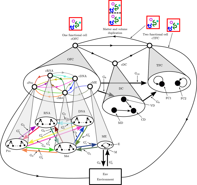
Figure 3: A hierarchical category to represent the living single cell (see text for explanation).

Most of the attempts done to describe single cells and bacteria from a theoretical and computational point of view[21, 22, 23], apply the modular cell biology approach[20]. In general, the description is at coarse-grained level and each module is treated with more detail (finer-level) using appropriate mathematical tools. The modules are finally integrated into a common computational frame[21].

In our description of the living single cell here we use instead the dynamical system theory for fuzzy hierarchical categories developed in previous Sections. The states of the cell are represented by fuzzy categories $\mathbf{\tilde{A}\in\tilde{C}=}\left[0,1\right]^{N}$ and we consider a dynamical system $\left(\mathbf{\tilde{C}},\mathcal{B},\mu,\mathcal{T}\right)$ with the action $\mathcal{T}=$ $\left(T^{n}:n\in\mathbb{N}\right)$. All the states $\mathbf{\tilde{A}}$ are supported by $X$ (Eq. 7) say, all they have the same elements $x=\left(a\overset{f}{\rightarrow}b\right)\mathbf{\in}X$ and differ among them in the membership degree of these elements (We call the vertices $a$ and $b$ the components and the composite objects $\left(a\overset{f}{\rightarrow}b\right)$ the elements of $\mathbf{\tilde{A}}$ or of their patterns).

In Fig. 3 we present the scheme we propose for the single cell which is valid for all the states (categories of $\mathbf{\tilde{C}}$) because, as was already mentioned, the different states distinguish themselves by just the membership degree of their elements. We can recognize three main levels.

The lower level (molecular level) shows five patterns labeled ME (for Matter and Energy); Met (for metabolism); DNA; RNA and Pro (for proteins). Except for ME in the other four patterns we have schematically drawn distinguished links among their components that, just for illustration, we have pictured with the same form. As we will see, the fine details at molecular and atomic level actually will be irrelevant for our analysis here. The pattern ME receives special attention because is through it that the cell relates with the environment, a relation that we want to emphasize. With DNA we mean all the information-carrying genetic apparatus, whereas RNA involves the whole translation machinery that transforms the genetic information into the complete set of ubiquitous polypeptides and proteins. On the other hand Met refers to the complex network of chemical reactions that get the molecules and energy necessary for the diverse modules can work.

The intermediate level (coarse-grained level) has three patterns denoted OFC (one functional cell); DC (duplicated cell) and TFC (two functional cells). The components of the pattern OFC are the colimits of the patterns at the lower level. We indicate in this figure the colimits with a small open circle. In all the cases the collective binding link from each pattern component to the corresponding colimit has been omitted in order to simplify the drawing.

The third level (cellular level) has only one pattern that consists of three components (cOFC, cDC, cTFC) which are just the colimits of the three patterns of the second level.

The patterns of a given level are related among them by mean of clusters whose definition we remember now[13]:

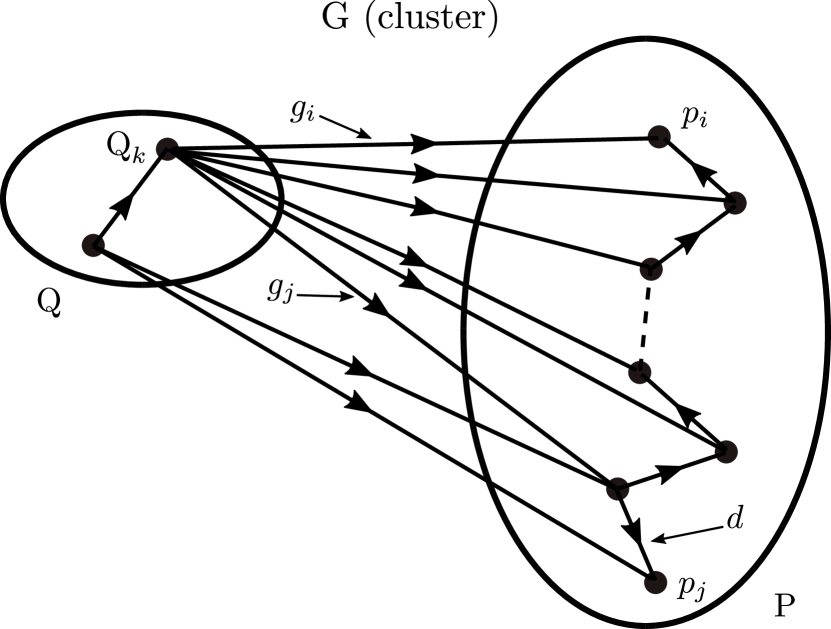
Figure 4: A cluster from the pattern Q to the pattern P.

Definition 11(see Fig.4). Given two patterns P and Q in a category, a cluster from Q to P is a maximal set of links between components of these patterns that satisfies the following conditions:

i) For each index $k$, the component Q_k of Q has at least one link to a component of P and  if there are several such links, they are correlated by a zigzag of distinguished links of P.

ii) The composite of a link of the cluster with a distinguished link of P (as $d$ in Fig. 4), or of a distinguished link of Q (v.g. the only one shown in Fig. 4) with a link of the cluster, also belongs to the cluster.

For simplicity, in Fig. 3, we have represented the whole set of links in each cluster with just a broad arrow labeled G${}_{\text{i}}$ and G${}_{\text{i}}^{\prime}$ (i $=0,1,2,\cdots,7$) and G${}_{8},$G₉ and G₁₀. Note that in correspondence with the clusters in a lower level we have links between the colimits of the corresponding patterns. In particular, in Fig. 3, the clusters between the pairs of patterns ME, Met, DNA, RNA and Pro have been drawn with different colors which are the same ones used for the links between colimits in the upper level.

In the APPENDIX A we explicit the elements considered in Fig. 3 for our model of living cell. The description is limited for simplicity to the intermediate and higher levels so that the collective binding links  $\left(c_{i}\right)_{i\in\mathbf{I}}$  from the patterns Met, DNA, RNA and Pro in the lower level to the corresponding colimits cMet, cDNA, cRNA and cPro, respectively, are not taken into account. In the same spirit we also ignore the internal structure of the clusters in the lower level. This means that we restrict ourselves to a coarse-grained description. This is a simplified version of the more realistic model we could hypothetically construct following the present approach (v.g. by introducing in detail the molecular level). Below we consider an even simpler version (toy model) that should make explicit calculations more accessible (Fig. 5).

Although the collective binding links  $\left(c_{i}\right)_{i\in\mathbf{I}}$  from the patterns OFC, CDF and TFC in the coarse-grained level to the corresponding colimits cOFC, cDC and cTFC, respectively, are not drawn in Fig. 3 they are explicitly considered in tables 2 - 7 of the APPENDIX A. Besides in tables 2 - 7 we take into account the possibility that between a source $a$ and a target $b$ be more than one arrow (which are differentiated with prime symbols). These elements mean either the indirect interaction between $a$ and $b$ via a third element $c$ or simply their direct interaction.

To give an explicit form for the map in Eq.14 that acts as the dynamic in our representation of the living single cell as a dynamical system, we previously define the subsets $\mathit{K}_{i}^{{\dagger}}$ and $\mathit{K}_{i}^{{\ddagger}}$ formed by those elements of the category that represents the cell which, in addition, are neighbors of the element $x_{i}$. We consider that a map $x_{r}$ is neighbor of the map $x_{i}$ if they have at least one vertex in common or, in other words, we take as neighbors of an element $\left(a\overset{f}{\rightarrow}b\right)$ all the elements which have at least one of $a$ and $b$ as source or target. In particular, we consider that each element is neighbor of itself. The subsets $\mathit{K}_{i}^{{\dagger}}$ and $\mathit{K}_{i}^{{\ddagger}}$ differ in that, whereas each element $x_{k}$ of $\mathit{K}_{i}^{{\ddagger}}$ can be expressed as product of two other elements $x_{k_{1}}$and $x_{k_{2}}$ of the category: $x_{k}=x_{k_{1}}\bullet x_{k_{2}}$,  the elements of $\mathit{K}_{i}^{{\dagger}}$ can not. Thus we take for the map:

$$\mathbf{\chi}_{\mathbf{B}}(x_{i}) =T_{i}\left(\mathbf{\chi}_{\mathbf{A}}(x_{i});\text{ }\left\{\mathbf{\chi}_{\mathbf{A}}(x_{j})\right\}_{j\neq i}\text{ }\right)\text{ \ }$$

$$=\left\{\begin{array}[c]{c}\text{ }\left(\sum\limits_{j\in\left\{j:\text{ }x_{j}\in\mathit{K}_{i}^{{\dagger}}\cup\mathit{K}_{i}^{{\ddagger}}\right\}}\varepsilon_{ij}\right)^{-1}\left(\text{\ }\sum\limits_{x_{j}\in\mathit{K}_{i}^{{\dagger}}}\varepsilon_{ij}r_{j}\mathbf{\chi}_{\mathbf{A}}(x_{j})\exp\left\{1-r_{j}\mathbf{\chi}_{\mathbf{A}}(x_{j})\right\}\right.\text{ \ \ \ \ \ \ \ \ \ \ \ \ \ \ \ \ \ \ \ \ \ \ \ \ \ \ \ \ \ \ \ \ \ \ \ \ \ \ \ \ \ \ \ \ \ \ \ \ \ }\\ \left.+\sum\limits_{x_{k}\in\mathit{K}_{i}^{{\ddagger}}}\varepsilon_{ik}r_{k}\min\left[\mathbf{\chi}_{\mathbf{A}}(x_{k_{1}}),\mathbf{\chi}_{\mathbf{A}}(x_{k_{2}})\right]\exp\left\{1-r_{k}\min\left[\mathbf{\chi}_{\mathbf{A}}(x_{k_{1}}),\mathbf{\chi}_{\mathbf{A}}(x_{k_{2}})\right]\right\}\right)\text{ \ \ \ \ \ \ \ \ \ \ \ \ \ \ \ \ \ \ \ \ \ \ \ \ \ \ }\\ \text{ \ \ \ \ \ \ \ \ \ \ \ \ \ \ \ \ \ \ \ \ \ \ \ \ \ \ \ \ \ \ \ \ \ \ \ \ \ \ if }x_{i}\text{ is not product of other two elements \ \ \ \ \ \ \ \ \ \ \ \ \ \ \ \ \ \ \ \ \ \ \ \ \ \ \ \ \ \ \ }\\ \min\left[\mathbf{\chi}_{\mathbf{B}}(x_{i_{1}}),\mathbf{\chi}_{\mathbf{B}}(x_{i_{2}})\right]\text{ \ \ \ \ \ \ \ \ \ \ \ \ \ \ \ \ \ \ \ \ \ \ \ \ \ \ \ \ \ \ \ \ \ \ \ \ \ \ \ \ \ \ \ \ \ \ \ \ \ \ \ \ \ \ \ \ \ \ \ \ \ \ \ \ \ \ \ \ \ \ \ \ \ \ \ \ \ \ \ \ \ \ \ \ \ \ \ \ \ \ \ \ \ \ \ \ \ \ \ \ \ \ \ }\\ \text{ \ \ \ \ \ \ \ \ \ \ \ \ \ \ \ \ \ \ \ \ if }x_{i}=x_{i_{1}}\bullet x_{i_{2}}\text{ \ \ \ \ \ \ \ \ \ \ \ \ \ \ \ \ \ \ \ \ \ \ \ \ \ \ \ \ \ \ \ \ \ \ \ \ \ \ \ \ \ \ \ \ \ \ \ \ }\end{array}\right.$$ (23)

where $i=1,2,\cdots,N$ and $\varepsilon_{ij}$ denotes the coupling between the element $x_{i}$ and its neighbor $x_{j}$. We see that Eq. 23 maps the domain $\left[0,1\right]^{N}$ into itself.

It is evident the resemblance of the map given by Eq. 23 with the Ricker map[25]. In fact, Eq. 23 can be thought of as a $N$-dimensional version of the one-dimensional Ricker map that additionally includes the composition law of fuzzy categories. We recall that the Ricker map (normalized in order to tranform into itself the interval $\left[0,1\right]$), say $x_{n+1}=rx_{n}\exp\left(1-rx_{n}\right)$ (see APPENDIX B) is in turn, a generalized version of the well known logistic-map[35] for population dynamics $x_{n+1}=ax_{n}\left(1-x_{n}\right)$. In both models, the population, initially small, has abundant resources to its disposal and grows. However, since the resources are limited, for a larger population the competition for food among its individuals causes that the death rate becomes higher than the birth rate and population decreases.

In our case the elements $x_{i}$ are the diverse activities and processes of the cell and the membership degree $\mathbf{\chi}_{\mathbf{A}}(x_{i})$ can be taken as a measure of their strength. For a given $x_{i}$,  when the membership values of itself and of its neighbors are small and increase we expect that they favour the process $x_{i}$ and then $\mathbf{\chi}_{\mathbf{B}}(x_{i})$ also grows. But, if these processes strengths follow growing beyond those values that allow a synchronized workings, then they become more a disturbance for $x_{i}$ than a positive contribution. A rough analogy of this situation can be found in the transit of a city crowded street. Each car individually can run at over say 150 Km/hour. However, given a car in the crowded street it is influenced by the others (particulary its neighbors) so will increase its velocity until an optimal one, say about 60 Km/hour, at which the car will move in harmony with the whole transit. If the chosen car or someone of its neighborhood increase the velocity over the optimal one then the considered car in particular and the transit in general will be perturbed in some way (vg. crashes) and, as a result, their velocity will diminish.

Our strategy consists, as we will discuss in next Subsection, into adjust the parameters in such a way that relevant aspects of the model (as describing a living cell) be fulfilled. However the huge number of parameters make any attempt in this direction a very hard task. To take an idea of the problem we remember that, in one, two and three dimensions, the logistic, Hénon and Lorenz classical dynamic maps have only one, two and three parameters, respectively. Dynamics in high dimensions with larger number of parameters are considered, for example, in ref. [36]

Any way, we consider that the model shown in Fig. 3 is still useful in the sense of providing a graphic description of a very complex system which, furthermore, can suggest simplified versions of the whole model (toy models) that allow to numerically study the single cell focusing into particular aspects of its behavior. In this spirit, in Fig. 5, we present a toy model of the living cell that emphasizes the binary fission. For this model, whose state space has dimension $N=4$, the map in Eq. 23 contains $n_{p}=14$ parameters to be determined: $r_{1}$, $r_{2}$, $r_{3}$, $r_{4}$, $\varepsilon_{11}$, $\varepsilon_{12}$, $\varepsilon_{14}$, $\varepsilon_{21}$, $\varepsilon_{22}$, $\varepsilon_{23}$, $\varepsilon_{24}$, $\varepsilon_{32}$, $\varepsilon_{33}$, $\varepsilon_{34}$ (see table 1 where we explicitly give the elements for the model of Fig. 5 together with their neighbors). The number of parameters for the model of Fig. 3, that has $N=108$ elements in each state (see tables 2 - 7 in the APPENDIX A), is several times greater than this. In Subsection C we reduce even more the number of parameters for the toy model by equaling some of the coupling parameters $\varepsilon_{ij}$.

4.2 Life and the edge of chaos

It is generally accepted that the notable stability of the living systems, say the capacity to support their temporal and spatial organization by adapting themselves to changes in the environment, is an indication that they evolve at the edge of chaos[26, 27, 28]. At the edge of chaos the system dynamics is characterized by the fact that the largest Lyapunov exponent is equal to zero. Within a hyperbolic dynamical systems framework, Pesin, Katok and Ruelle have proved that negative Lyapunov exponents correspond to global stable manifolds or contracting directions, and positive Lyapunov exponents correspond to global unstable manifolds or expanding directions[37, 38, 39]. In general, a zero exponent corresponds to a neutral direction, a situation that can be observed in partially hyperbolic diffeomorphisms[40, 41]. For these, the tangent bundle $TM$ can be split into three invariant continuous subbundles: $TM=E^{s}\oplus E^{c}\oplus E^{u}$, where $E^{s}$, $E^{u}$ denote the strongly stable and unstable (respectively) subspaces and $E^{c}$ the central subspace in which contractions and expansions are weaker. Under certain conditions has been proved that the largest Lyapunov exponent in this region is zero[42].

Thus, from the dynamical systems theory point of view, we take the largest Lyapunov exponent equal to zero as being the main characteristic of the living systems and use this property to determine the unknown parameters in the map of Eq. 23.

On the other hand, if we define $DT_{\mathbf{\tilde{B}}}^{k}$ (see Eq. 18) as the product of derivatives along the orbit:

$$DT_{\mathbf{\tilde{B}}}^{k}=DT_{\mathbf{\tilde{B}}_{k-1}}\cdots DT_{\mathbf{\tilde{B}}_{0}},$$ (24)

where $\mathbf{\tilde{B}}_{j}=T^{j}\left(\mathbf{\tilde{B}}\right)$, then Kingman´s subadditive ergodic theorem[43] says that $\lim_{k\rightarrow\infty}\frac{1}{k}\log\left(\left\|DT_{\mathbf{\tilde{B}}}^{k}\right\|\right)$ exists for almost all points $\mathbf{\tilde{B}}$. Besides, since[34]

$$\underset{k\rightarrow\infty}{\lim\sup}\frac{1}{k}\log\left\|DT_{\mathbf{\tilde{B}}}^{k}\mathbf{v}\right\|\leq\lim_{k\rightarrow\infty}\frac{1}{k}\log\left\|DT_{\mathbf{\tilde{B}}}^{k}\right\|,$$ (25)

we have for the largest Lyapunov exponent:

$$\lambda_{\max}\left(\mathbf{\tilde{B}}\right)=\lim_{k\rightarrow\infty}\frac{1}{k}\log\left\|DT_{\mathbf{\tilde{B}}}^{k}\right\|.$$ (29)

Therefore, according to our assumption, the condition of life at the edge of the chaos would imply that the right hand side of Eq. 29 is equal to zero.

In order to determine the $n_{p\text{ }}$parameters of the map in Eq.(23) we propose to solve the system of non linear equations $\lambda_{\max}\left(\mathbf{\tilde{B}}_{\alpha}\right)=0$ for $n_{i}$ initial states $\mathbf{\tilde{B}}_{\alpha}$ ($\alpha=1,2,\cdots,n_{i}$). Optimization technics such as genetic algorithms[44, 45] or the particle swarm optimization procedure[46] seem adequate to numerically find them by using as fitness functions these equations. Of course the condition $\lambda_{\max}\left(\mathbf{\tilde{B}}_{\alpha}\right)=0$ must be interpreted, from a numerical point of view, in the sense of Lyapunov exponent zero-crossing[47]. We must also mention the possibility that the diverse initial conditions $\mathbf{\tilde{B}}_{\alpha}$ ($\alpha=1,2,\cdots,n_{i}$) evolves towards distinct attractors, so we consider all the attractors as describing our cell if, for each $\mathbf{\tilde{B}}_{\alpha}$, the corresponding maximun Lyapunov exponent is zero.

4.3 Toy model for the cellular fission

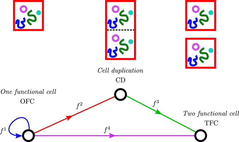
Figure 5: Toy model for the living single cell, with emphasis on the cellular fission, obtained as a drastic simplification of the more complete model of Fig. 3.

$x_{i}$	neighbors
$x_{1}=\text{OFC}\overset{f_{1}}{\rightarrow}\text{OFC}$	$x_{1},x_{2},x_{4}$
$x_{2}=\text{OFC}\overset{f_{2}}{\rightarrow}\text{CD}$	$x_{1},x_{2},x_{3},x_{4}$
$x_{3}=\text{CD}\overset{f_{3}}{\rightarrow}\text{TFC}$	$x_{2},x_{3},x_{4}$
$x_{4}=\text{OFC}\overset{f_{4}}{\rightarrow}\text{TFC}=x_{3}\bullet x_{2}$	$x_{1},x_{2},x_{3},x_{4}$

Table 1: Elements of the toy model of Fig. 5 and their neighbors.

In Fig. 5 we show the toy model we propose to describe, within our formalism, the cellular division of a bacterium[48],[49]. It approximately corresponds to the higher level in the hierarchical category displayed in Fig. 3 to represent a living single cell. Their elements, with the corresponding neighbors, are listed in table 1.

In the model, the element $x_{1}$= OFC $\overset{f_{1}}{\rightarrow}$ OFC accounts for the normal workings of a single cell. It includes all the operations that allow the cell functions along the whole life cycle. The element $x_{2}$= OFC $\overset{f_{2}}{\rightarrow}$ CD denotes the duplication of the bacterium chromosome and molecules as well as the mechanisms that double the bacterium size, all these resulting into the FtsZ ring formation and the divisome assembly. The element $x_{3}$= CD $\overset{f_{3}}{\rightarrow}$ TFC, on the other hand, is associated with the division or splitting of the living cell into two identical ones. Finally, $x_{4}$= OFC $\overset{f_{4}}{\rightarrow}$ TFC = $x_{3}\bullet x_{2}$ represents the composition of both, the cell matter-volume duplication and its separation into two daughters cells so describing, in a unique process, the transformation of a single bacterium into a pair of bacteria equal to that one.

At a given time our system is represented as a fuzzy category or, according to previous comments, as a point $\mathbf{\tilde{A}=}$ $\left(\mathbf{\chi}_{\mathbf{A}}(x_{1}),\mathbf{\chi}_{\mathbf{A}}(x_{2}),\mathbf{\chi}_{\mathbf{A}}(x_{3}),\mathbf{\chi}_{\mathbf{A}}(x_{4})\text{ }\right)$ $\mathbf{\in}$ $\left[0,1\right]^{4}$ (see Eq.11). We remember that the membership degree $\mathbf{\chi}_{\mathbf{A}}(x_{i})$ denotes the strength or powerful of the element (activity or process) $x_{i}$ ($i=1,2,3,4$).

The system evolves with time through a sequence of categories driven by the transformation given by Eq. (23) with the $n_{p}=14$ parameters

$$r_{1},r_{2},r_{3},r_{4},\varepsilon_{11},\varepsilon_{12},\varepsilon_{14},\varepsilon_{21},\varepsilon_{22},\varepsilon_{23},\varepsilon_{24},\varepsilon_{32},\varepsilon_{33},\varepsilon_{34}$$

taking values such that the system to be at the edge of the chaos so that the corresponding Lyapunov exponent, evaluated by Eq. 29, equals zero. Despite the drastic simplification, with respect to the general model of Fig. 3, implied by the toy model considered here, it even involves a number of parameters which is large enough as to make the associated dynamics very complex. In particular, the simultaneous determinations of the $n_{p\text{ }}$parameters of the map in Eq.(23) is still a hard task. So, here, in order to exemplify the kind of information we can extract from the model, we relax the requirement and demand that the condition $\lambda_{\max}\left(\mathbf{\tilde{B}}_{\alpha}\right)=0$ be fulfilled for just one initial condition. Thus we fix all the parameters except one, say $r_{3}$, to some reasonable values which are suggested by the analysis of the one-dimensional Ricker map and by the assumption that the membership value of the element $x_{i}$ at a given time instant, is mainly influenced by its membership value at the previous iteration and, at less extent, by the membership values of their neighbors also at the previous time instant. We specifically choose: $r_{1}=1.0$, $r_{2}=2.5$, $r_{4}=4.6$ . Besides, to simplify even more the model, we take all the diagonal coupling parameters equal to one and all the off-diagonal coupling parameters equal to $10^{-3}$: $\varepsilon_{ii}=1$ ($i=1,2,3$) and $\varepsilon_{ij}=\varepsilon=0.001$ ($i\neq j$; $i=1,2,3$; $j$ such that $x_{j}$ is neighbor of $x_{i}$). Finally, the parameter $r_{3}$ will be chosen by requiring that the system maximum Lyapunov exponent equals zero.

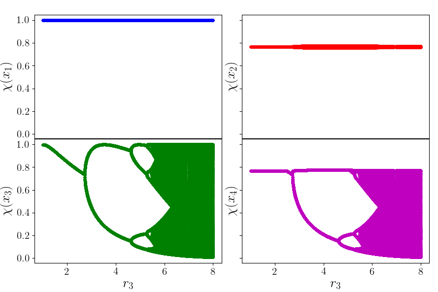
Figure 6: Bifurcation diagrams for $\mathbf{\chi}(x_{i})$ ($i=1,2,3,4$) as a function of $r_{3}$.

In Fig. 6 we show the bifurcation diagrams for $\mathbf{\chi}(x_{i})$ ($i=1,2,3,4$) as a function of $r_{3}$ with the remainder parameters fixed at the indicated values. The corresponding curve for the maximum Lyapunov exponent is given in Fig. 7.

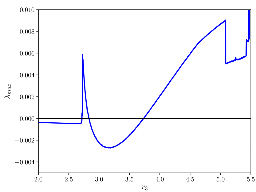
Figure 7: Maximum Lyapunov exponent $\lambda_{\max}$ as a function of the parameter $r_{3}$.

The bifurcation diagrams for $\mathbf{\chi}(x_{1})$ and $\mathbf{\chi}(x_{2})$ show a period-$2$ cycle along the considered range of $r_{3}$ values, the two branches being very near one of the other, specially in the case of $\mathbf{\chi}(x_{1})$. The diagram for $\mathbf{\chi}(x_{3})$ shows a richer structure with successive bifurcations corresponding to $2^{n}$-cycles ($n=1,2,3,...$). These bifurcations come faster and faster resulting into a cascade. Taking into account the small values we are considering for the off-diagonal coupling parameters $\varepsilon_{3j}$ is natural that this diagram to be very similar to that obtained for the one-dimensional Ricker map as a function of its parameters $r$ (see APPENDIX B). The diagram for $\mathbf{\chi}(x_{4})$, on the other hand, is determined by the composition law between $\mathbf{\chi}(x_{2})$ and $\mathbf{\chi}(x_{3})$.

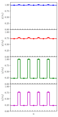
Figure 8: Discrete trajectories $\mathbf{\chi}(x_{i})$ ($i=1,2,3,4$) vs. $n$ (full circles). Solid lines: continuous representation.

¿From the Lyapunov exponent curve (Fig. 7), we take for the parameter $r_{3}$ the value $3.73$. Around this value, $\lambda_{\max}$ changes from being negative to positive, that is to say the system is at the edge of the chaos. With $r_{3}=3.73$ and the remainder parameters chosen as indicated before, we calculate the trajectories $\mathbf{\chi}(x_{i})$ ($i=1,2,3,4$) vs. $n$ ($n$ = number of iterations) determined, in our discrete representation, by the full circles of Fig. 8. In order to interpret this trajectories in terms of the biological phenomena in which we are interested, we represent the (continuous) temporal evolution of the $\mathbf{\chi}(x_{i})\acute{}s$ with the solid lines. We assume that the interval of time that demands the proper duplication is several times smaller than the time the cell needs to prepare itself for that event.

We observe that the four curves are periodic of period $2$. For $\mathbf{\chi}(x_{1})$ the variation within each period is very small. The same occurs for $\mathbf{\chi}(x_{2})$ although here the difference is most notable. Actually, the values $r_{1}=1.0$ and $r_{2}=2.5$ would correspond in the case of a single Ricker map (see Fig. 9b in the APPENDIX B) to a steady state (fixed point) at $\mathbf{\chi}(x_{1})\approx 1.0$ and $\mathbf{\chi}(x_{2})\approx$ $0.75$, respectively. The small variations, giving period-$2$ curves, are due to the coupling with the other elements in the generalized map of Eq. 23. We interpret this behavior of $\mathbf{\chi}(x_{1})$ as that the cell works practically at full along its life cycle. Most of the workings is addressed to prepare the bacterium to his division, so, although to a lesser strength, $x_{2}$ works almost constant too, increasing a little its power in the second part of the period. For $r_{3}=3.73$ the bifurcation diagram of the Fig. 9b in the APPENDIX B gives a period-$2$ cycle with the upper and lower values at about $0.95$ and $0.24$, respectively which are practically the values observed in Fig. 8 for $\mathbf{\chi}(x_{3})$, the effect of the coupling with the other elements being very small. The explanation we can give for the jump between the first and the second part of the period is that during the first part the divisome is not yet completely formed and the division works at full just in the second part. Finally $\mathbf{\chi}(x_{4})$, the curve that globally describe the binary fission, results of the composition of $\mathbf{\chi}(x_{2})$ and $\mathbf{\chi}(x_{3})$ taking, between both values, the minimum one so that it oscillates between $0.77$ and $0.23$.

5 Conclusions

In this work we have improved the theory of hierarchical evolutive systems of Ehresmann and Vandremeersch by adding the concept of fuzzy categories. This way each category $\mathbf{\tilde{A}}$ can be represented as a point in a states space $\left[0,1\right]^{N}$ $\subset$ $\mathbb{R}^{N}$ where $N$ is the space dimension. The coordinates of the points in this space are the membership values associated with the category components. Within this context, the state of the system under study at a given time is described by a hierarchical fuzzy category $\mathbf{\tilde{A}}_{h}$ where the element $x_{i}=a\overset{f_{i}}{\rightarrow}b$ represents the relation between the system components $a$ and $b$ mediated by the function $f_{i}$ and $\mathbf{\chi}_{\mathbf{A}}(x_{i})$ the strength or powerful of this relation at that time. In our discrete time description, the temporal evolution of the system is accounted by a sequence of fuzzy categories $\left\{\left(\mathbf{\tilde{A}}_{h}\right)_{n}\right\}_{n\in\mathbb{N}}$ all whose members have the same elements $x_{i}$ differing in their membership values $\mathbf{\chi}(x_{i})$ ($i=1,2,\cdots,N$), so that the functor that transforms the category $\left(\mathbf{\tilde{A}}_{h}\right)_{n}$ into the category $\left(\mathbf{\tilde{A}}_{h}\right)_{n+1}$ is determined by simply giving the maps that transform $\mathbf{\chi}_{\left(\mathbf{A}\right)_{n}}(x_{i})$ into $\mathbf{\chi}_{\left(\mathbf{A}\right)_{n+1}}(x_{i})$ say: $\mathbf{\chi}_{\left(\mathbf{A}\right)_{n+1}}(x_{i})=T_{i}\left(\mathbf{\chi}_{\left(\mathbf{A}\right)_{n}}(x_{i});\text{ }\left\{\mathbf{\chi}_{\left(\mathbf{A}\right)_{n}}(x_{j})\right\}_{j\neq i}\text{ }\right)$ ($i=1,2,\cdots,N$). If we consider for the $T_{i}\acute{}s$ adequate diffeomorphisms, then we can make contact with the theory of dynamical systems an use all its tools to describe the behavior of the system with time. In this manner a quantification of the hierarchical evolutive systems theory is achieved.

Here we have applied our formalism to describe the living single cell for which we propose a quite general hierarchical category to represent its state at a given time and have proposed as dynamics parametrized transformations $T_{i}$ based on the Ricker map. Also we suggest that the parameters be determined under the condition that the system evolves at the edge of the chaos, a property generally taken as hallmark of the life. To exemplify the theory we have drastically simplified the model into a toy model with dimension $4$ that emphasizes the cellular fission. However we think that the formalism is applicable to other biological phenomena as well as to diverse economic and social problems and, in general, to complex systems for which the ordinary mathematical tools are hard to use. Of course the choice of the maps to be used as dynamics and the conditions that determine the parameters will depend on the particular problem to be studied.

Acknowledgments

Support of this work by Universidad Nacional de La Plata, Universidad Nacional de Rosario and Consejo Nacional de Investigaciones Científicas y Técnicas of Argentina is greatly appreciated. C.M.C. and F.V. are a member and a researcher under contract, respectively, of CONICET.

APPENDIX A: Elements of the living cell model given by Fig. 3

In tables 2 - 7 we explicitly show the elements involved in the living single cell model drawn in Fig. 3. To make the presentation more clear we collect in table 2 the elements that relate the cell with the environment, in table 3 and 4, respectively, the elements of the patterns that determine the colimits cOFC and cDC, cTFC; in tables 5, 6 those involved in the cluster G${}_{\text{8}}$ and clusters G${}_{\text{9}}$, G${}_{\text{10}}$, repectively, and finally in table 7 the maps linking the colimits cOFC, cDC and cTFC which accounts for the binary fission.

Elements that differ in a prime symbol (non prime, prime, double prime) have the same source and target (and thus the same neighbors) but distinct maps. When it corresponds we have indicated the product of elements given by the composition law.

$x_{i}$	$x_{i}$
$x_{1}=\text{Env}\overset{f_{1}}{\rightarrow}\text{M}$	$x_{2}=\text{Env}\overset{f_{2}}{\rightarrow}\text{E}$
$x_{1}^{\prime}=\text{Env}\overset{f_{1}^{\prime}}{\rightarrow}\text{M}=x_{6}\bullet x_{2}$	$x_{2}^{\prime}=\text{Env}\overset{f_{2}^{\prime}}{\rightarrow}\text{E}=x_{5}\bullet x_{1}$
$x_{3}=\text{M}\overset{f_{3}}{\rightarrow}\text{Env}$	$x_{4}=\text{E}\overset{f_{4}}{\rightarrow}\text{Env}$
$x_{3}^{\prime}=\text{M}\overset{f_{3}^{\prime}}{\rightarrow}\text{Env}=x_{4}\bullet x_{5}$	$x_{4}^{\prime}=\text{E}\overset{f_{4}^{\prime}}{\rightarrow}\text{Env}=x_{3}\bullet x_{6}$
$x_{5}=\text{M}\overset{f_{5}}{\rightarrow}\text{E}$	$x_{6}=\text{E}\overset{f_{6}}{\rightarrow}\text{M}$
$x_{5}^{\prime}=\text{M}\overset{f_{5}^{\prime}}{\rightarrow}\text{E}=x_{2}\bullet x_{3}$	$x_{6}^{\prime}=\text{E}\overset{f_{6}^{\prime}}{\rightarrow}\text{M}=x_{1}\bullet x_{4}$
$x_{7}=\text{M}\overset{f_{7}}{\rightarrow}\text{cME}$	$x_{8}=\text{E}\overset{f_{8}}{\rightarrow}\text{cME}$
$x_{9}=\text{cPro}\overset{f_{9}}{\rightarrow}\text{Env}$

Table 2: Elements relating the cell and the environment.

$x_{i}$	$x_{i}$
$x_{10}=\text{cME}\overset{f_{10}}{\rightarrow}\text{cMet}$	$x_{11}=\text{cMet}\overset{f_{11}}{\rightarrow}\text{cME}$
$x_{12}=\text{cMet}\overset{f_{12}}{\rightarrow}\text{cDNA}$	$x_{13}=\text{cDNA}\overset{f_{13}}{\rightarrow}\text{cMet}$
$x_{12}^{\prime}=\text{cMet}\overset{f_{12}^{\prime}}{\rightarrow}\text{cDNA}=x_{19}\bullet x_{14}$	$x_{13}^{\prime}=\text{cDNA}\overset{f_{13}^{\prime}}{\rightarrow}\text{cMet}=x_{15}\bullet x_{18}$
$x_{12}^{\prime\prime}=\text{cMet}\overset{f_{12}^{\prime\prime}}{\rightarrow}\text{cDNA}=x_{21}\bullet x_{16}$	$x_{13}^{\prime\prime}=\text{cDNA}\overset{f_{13}^{\prime\prime}}{\rightarrow}\text{cMet}=x_{17}\bullet x_{20}$
$x_{14}=\text{cMet}\overset{f_{14}}{\rightarrow}\text{cRNA}$	$x_{15}=\text{cRNA}\overset{f_{15}}{\rightarrow}\text{cMet}$
$x_{14}^{\prime}=\text{cMet}\overset{f_{14}^{\prime}}{\rightarrow}\text{cRNA}=x_{18}\bullet x_{12}$	$x_{15}^{\prime}=\text{cRNA}\overset{f_{15}^{\prime}}{\rightarrow}\text{cMet}=x_{13}\bullet x_{19}$
$x_{14}^{\prime\prime}=\text{cMet}\overset{f_{14}^{\prime\prime}}{\rightarrow}\text{cRNA}=x_{23}\bullet x_{16}$	$x_{15}^{\prime\prime}=\text{cRNA}\overset{f_{15}^{\prime\prime}}{\rightarrow}\text{cMet}=x_{17}\bullet x_{22}$
$x_{16}=\text{cMet}\overset{f_{16}}{\rightarrow}\text{cPro}$	$x_{17}=\text{cPro}\overset{f_{17}}{\rightarrow}\text{cMet}$
$x_{16}^{\prime}=\text{cMet}\overset{f_{16}^{\prime}}{\rightarrow}\text{cPro}=x_{22}\bullet x_{14}$	$x_{17}^{\prime}=\text{cPro}\overset{f_{17}^{\prime}}{\rightarrow}\text{cMet}=x_{15}\bullet x_{23}$
$x_{16}^{\prime\prime}=\text{cMet}\overset{f_{16}^{\prime\prime}}{\rightarrow}\text{cPro}=x_{20}\bullet x_{12}$	$x_{17}^{\prime\prime}=\text{cPro}\overset{f_{17}^{\prime\prime}}{\rightarrow}\text{cMet}=x_{13}\bullet x_{21}$
$x_{18}=\text{cDNA}\overset{f_{18}}{\rightarrow}\text{cRNA}$	$x_{19}=\text{cRNA}\overset{f_{19}}{\rightarrow}\text{cDNA}$
$x_{18}^{\prime}=\text{cDNA}\overset{f_{18}^{\prime}}{\rightarrow}\text{cRNA}=x_{14}\bullet x_{13}$	$x_{19}^{\prime}=\text{cRNA}\overset{f_{19}^{\prime}}{\rightarrow}\text{cDNA}=x_{12}\bullet x_{15}$
$x_{18}^{\prime\prime}=\text{cDNA}\overset{f_{18}^{\prime\prime}}{\rightarrow}\text{cRNA}=x_{23}\bullet x_{20}$	$x_{19}^{\prime\prime}=\text{cRNA}\overset{f_{19}^{\prime\prime}}{\rightarrow}\text{cDNA}=x_{21}\bullet x_{22}$
$x_{20}=\text{cDNA}\overset{f_{20}}{\rightarrow}\text{cPro}$	$x_{21}=\text{cPro}\overset{f_{21}}{\rightarrow}\text{cDNA}$
$x_{20}^{\prime}=\text{cDNA}\overset{f_{20}^{\prime}}{\rightarrow}\text{cPro}=x_{16}\bullet x_{13}$	$x_{21}^{\prime}=\text{cPro}\overset{f_{21}^{\prime}}{\rightarrow}\text{cDNA}=x_{12}\bullet x_{17}$
$x_{20}^{\prime\prime}=\text{cDNA}\overset{f_{20}^{\prime\prime}}{\rightarrow}\text{cPro}=x_{22}\bullet x_{18}$	$x_{21}^{\prime\prime}=\text{cPro}\overset{f_{21}^{\prime\prime}}{\rightarrow}\text{cDNA}=x_{19}\bullet x_{23}$
$x_{22}=\text{cRNA}\overset{f_{22}}{\rightarrow}\text{cPro}$	$x_{23}=\text{cPro}\overset{f_{23}}{\rightarrow}\text{cRNA}$
$x_{22}^{\prime}=\text{cRNA}\overset{f_{22}^{\prime}}{\rightarrow}\text{cPro}=x_{16}\bullet x_{15}$	$\text{ }x_{23}^{\prime}=\text{cPro}\overset{f_{23}^{\prime}}{\rightarrow}\text{cRNA}=x_{14}\bullet x_{17}$
$x_{22}^{\prime\prime}=\text{cRNA}\overset{f_{22}^{\prime\prime}}{\rightarrow}\text{cPro}=x_{20}\bullet x_{21}$	$x_{23}^{\prime\prime}=\text{cPro}\overset{f_{23}^{\prime\prime}}{\rightarrow}\text{cRNA}=x_{18}\bullet x_{21}$
$x_{24}=\text{cME}\overset{f_{24}}{\rightarrow}\text{cME}$	$x_{25}=\text{cMet}\overset{f_{25}}{\rightarrow}\text{cMet}$
$x_{26}=\text{cDNA}\overset{f_{26}}{\rightarrow}\text{cDNA}$	$x_{27}=\text{cRNA}\overset{f_{27}}{\rightarrow}\text{cRNA}$
$x_{28}=\text{cPro}\overset{f_{28}}{\rightarrow}\text{cPro}$	$x_{29}=\text{cME}\overset{f_{29}}{\rightarrow}\text{cOFC}$
$x_{30}=\text{cMet}\overset{f_{30}}{\rightarrow}\text{cOFC}$	$\text{ }x_{31}=\text{cDNA}\overset{f_{31}}{\rightarrow}\text{cOFC}$
$x_{32}=\text{cRNA}\overset{f_{32}}{\rightarrow}\text{cOFC}$	$x_{33}=\text{cPro}\overset{f_{33}}{\rightarrow}\text{cOFC}$

Table 3: Elements of the patterns determining cOFC.

$x_{i}$	$x_{i}$
$x_{34}=\text{MD}\overset{f_{34}}{\rightarrow}\text{CD}$	$x_{35}=\text{VD}\overset{f_{35}}{\rightarrow}\text{CD}$
$x_{36}=\text{CD}\overset{f_{36}}{\rightarrow}\text{cDC}$	$x_{37}=\text{MD}\overset{f_{37}}{\rightarrow}\text{cDC}=x_{36}\bullet x_{34}$
$x_{38}=\text{VD}\overset{f_{38}}{\rightarrow}\text{cDC}=x_{36}\bullet x_{35}$	$x_{39}=\text{FC1}\overset{f_{39}}{\rightarrow}\text{FC1}$
$x_{40}=\text{FC2}\overset{f_{40}}{\rightarrow}\text{FC2}$	$x_{41}=\text{FC1}\overset{f_{41}}{\rightarrow}\text{cTFC}$
$x_{42}=\text{FC2}\overset{f_{42}}{\rightarrow}\text{cTFC}$

Table 4: Elements of the patterns determining cDC and cTFC.

$x_{i}$	$x_{i}$
$x_{43}=\text{cME}\overset{f_{43}}{\rightarrow}\text{MD}$	$x_{44}=\text{cME}\overset{f_{44}}{\rightarrow}\text{VD}$
$x_{45}=\text{cME}\overset{f_{45}}{\rightarrow}\text{CD}$	$x_{46}=\text{cMet}\overset{f_{46}}{\rightarrow}\text{MD}$
$x_{47}=\text{cMet}\overset{f_{47}}{\rightarrow}\text{VD}$	$x_{48}=\text{cMet}\overset{f_{48}}{\rightarrow}\text{CD}$
$x_{49}=\text{cDNA}\overset{f_{49}}{\rightarrow}\text{MD}$	$x_{50}=\text{cDNA}\overset{f_{50}}{\rightarrow}\text{VD}$
$x_{51}=\text{cDNA}\overset{f_{51}}{\rightarrow}\text{CD}$	$x_{52}=\text{cRNA}\overset{f_{52}}{\rightarrow}\text{MD}$
$x_{53}=\text{cRNA}\overset{f_{53}}{\rightarrow}\text{VD}$	$x_{54}=\text{cRNA}\overset{f_{54}}{\rightarrow}$
$x_{55}=\text{cPro}\overset{f_{55}}{\rightarrow}\text{MD}$	$x_{56}=\text{cPro}\overset{f_{56}}{\rightarrow}\text{VD}$
$x_{57}=\text{cPro}\overset{f_{57}}{\rightarrow}\text{CD}$

Table 5: Elements of the clusters G${}_{\text{8}}$.

$x_{i}$	$x_{i}$
$x_{58}=\text{MD}\overset{f_{58}}{\rightarrow}\text{FC1}$	$x_{59}=\text{MD}\overset{f_{59}}{\rightarrow}\text{FC2}$
$x_{60}=\text{VD}\overset{f_{60}}{\rightarrow}\text{FC1}$	$x_{61}=\text{VD}\overset{f_{61}}{\rightarrow}\text{FC2}$
$x_{62}=\text{CD}\overset{f_{62}}{\rightarrow}\text{FC1}$	$4x_{63}=\text{CD}\overset{f_{63}}{\rightarrow}\text{FC}$
$x_{64}=\text{cME}\overset{f_{64}}{\rightarrow}\text{FC1}$	$x_{65}=\text{cME}\overset{f_{65}}{\rightarrow}\text{FC2}$
$x_{66}=\text{cMet}\overset{f_{66}}{\rightarrow}\text{FC1}$	$x_{67}=\text{cMet}\overset{f_{67}}{\rightarrow}\text{FC2}$
$x_{68}=\text{cDNA}\overset{f_{68}}{\rightarrow}\text{FC1}$	$x_{69}=\text{cDNA}\overset{f_{69}}{\rightarrow}\text{FC2}$
$x_{70}=\text{cRNA}\overset{f_{70}}{\rightarrow}\text{FC1}$	$x_{71}=\text{cRNA}\overset{f_{71}}{\rightarrow}\text{FC2}$
$x_{72}=\text{cPro}\overset{f_{72}}{\rightarrow}\text{FC1}$	$x_{73}=\text{cPro}\overset{f_{73}}{\rightarrow}\text{FC2}$

Table 6: Elements of the clusters G${}_{\text{9}}$ and G${}_{\text{10}}$.

$x_{i}$	$x_{i}$
$x_{74}=\text{cOFC}\overset{f_{74}}{\rightarrow}\text{cDC}$	$x_{75}=\text{cDC}\overset{f_{75}}{\rightarrow}\text{cTFC}$
$x_{76}=\text{cOFC}\overset{f_{76}}{\rightarrow}\text{cTFC}$	$x_{77}=\text{cTFC}\overset{f_{77}}{\rightarrow}\text{cOFC}$
$x_{78}=\text{cTFC}\overset{f_{78}}{\rightarrow}\text{Env}$

Table 7: Elements accounting for the binary fission.

APPENDIX B: The Ricker map

In Fig. 9(a) we show the Ricker map normalized to transform the interval $\left[0,1\right]$ into itself, say

$$x_{n+1}=rx_{n}\exp\left(1-rx_{n}\right),$$

with the parameter $r$ taking the values used in the text. Fig. 9(b), on the other hand, shows the corresponding bifurcation diagram for $r\in\left[1,8\right]$.

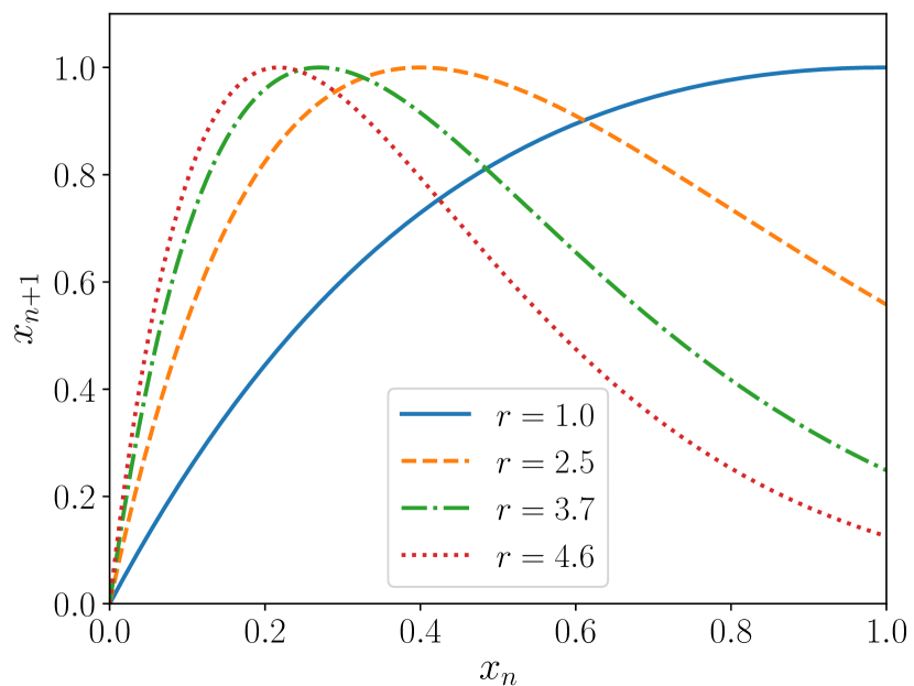
(a)

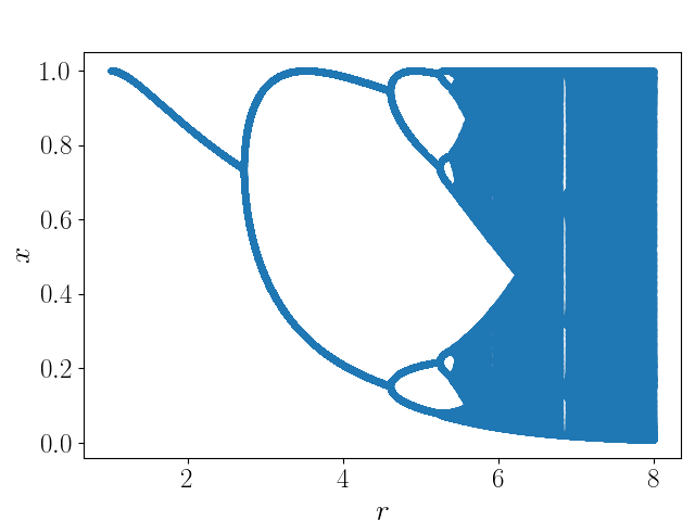
(b)

Figure 9: Panel a: Discrete trajectories $\mathbf{\chi}(x_{i})$ ($i=1,2,3,4$) vs. $n$ (full circles). Solid lines: continuous representation. Panel b: Bifurcation diagram for a single normalized Ricker map.

References

References

- [1] R. Badii, A. Politi, Complexity. Cambridge Nonlinear Science Series 6, Cambridge, UK: Cambridge University Press, 1997.
- [2] G. Gallavotti, Statistical mechanics, Springer-Verlag, Berlin Heidelberg, 1999.
- [3] J. Honerkamp, Estimation of Parameters, Springer Berlin Heidelberg, Berlin, Heidelberg, 2002, pp. 309–337. doi:10.1007/978-3-662-04763-7_8.
- [4] N. H. Packard, Complexity of growing patterns in cellular automata, Tech. rep., Princeton Univ. Inst. Adv. Stud., Princeton, NJ (Jan 1984).
- [5] M. Mitchell, J. P. Crutchfield, P. T. Hraber, Evolving cellular automata to perform computations: mechanisms and impediments, Physica D: Nonlinear Phenomena 75 (1) (1994) 361 – 391. doi:https://doi.org/10.1016/0167-2789(94)90293-3.
- [6] J. R. Dorfman, An Introduction to Chaos in Nonequilibrium Statistical Mechanics (Cambridge Lecture Notes in Physics), Cambridge University Press, 1999.
- [7] L. von Bertalanffy, General system theory: Foundations, development, applications (Penguin university books), Penguin, 1973.
- [8] N. Rashevsky, Topology and life: In search of general mathematical principles in biology and sociology, The bulletin of mathematical biophysics 16 (4) (1954) 317–348. doi:10.1007/BF02484495.
- [9] R. Rosen, A relational theory of biological systems, The bulletin of mathematical biophysics 20 (3) (1958) 245–260. doi:10.1007/BF02478302.
- [10] R. Rosen, A relational theory of biological systems ii, The bulletin of mathematical biophysics 21 (2) (1959) 109–128. doi:10.1007/BF02476354.
- [11] S. Eilenberg, S. MacLane, General theory of natural equivalences, Transactions of the American Mathematical Society 58 (2) (1945) 231–294.
- [12] A. Ehresmann, J.-P. Vanbremeersch, Hierarchical evolutive systems: A mathematical model for complex systems, Bulletin of Mathematical Biology 49 (1) (1987) 13 – 50. doi:https://doi.org/10.1016/S0092-8240(87)80033-2.
- [13] A. Ehresmann, J. Vanbremeersch, Memory Evolutive Systems; Hierarchy, Emergence, Cognition, Volume 4 (Studies in Multidisciplinarity), Elsevier Science, 2007.
- [14] A. Katok, B. Hasselblatt, Introduction to the Modern Theory of Dynamical Systems (Encyclopedia of Mathematics and its Applications), Cambridge University Press, 1996.
- [15] M. Behrisch, S. Kerkhoff, R. Pöschel, F. M. Schneider, S. Siegmund, Dynamical systems in categories, Applied Categorical Structures 25 (1) (2017) 29–57. doi:10.1007/s10485-015-9409-8.
- [16] G. Dimitrov, F. Haiden, L. Katzarkov, M. Kontsevich, Dynamical systems and categories, arXiv preprint arXiv:1307.8418 [math.CT].
- [17] B. P. Zeigler, R. Weinberg, System theoretic analysis of models: Computer simulation of a living cell, Journal of Theoretical Biology 29 (1) (1970) 35 – 56. doi:https://doi.org/10.1016/0022-5193(70)90117-7.
- [18] M. M. Domach, S. K. Leung, R. E. Cahn, G. G. Cocks, M. L. Shuler, Computer model for glucose-limited growth of a single cell of escherichia coli b/r-a, Biotechnology and Bioengineering 26 (3) (1984) 203–216. doi:10.1002/bit.260260303.
- [19] E. V. Nikolaev, J. C. Atlas, M. L. Shuler, Computer models of bacterial cells: from generalized coarsegrained to genome-specific modular models, Journal of Physics: Conference Series 46 (1) (2006) 322.
- [20] L. H. Hartwell, J. J. Hopfield, S. Leibler, A. W. Murray, From molecular to modular cell biology, Nature 402 (6761supp) (1999) C47–C52. doi:10.1038/35011540.
- [21] M. W. Covert, N. Xiao, T. J. Chen, J. R. Karr, Integrating metabolic, transcriptional regulatory and signal transduction models in escherichia coli, Bioinformatics 24 (18) (2008) 2044–2050. arXiv:/oup/backfile/content_public/journal/bioinformatics/24/18/10.1093_bioinformatics_btn352/2/btn352.pdf, doi:10.1093/bioinformatics/btn352.
- [22] J. Karr, J. Sanghvi, D. Macklin, M. Gutschow, J. Jacobs, B. Bolival, N. Assad-Garcia, J. Glass, M. Covert, A whole-cell computational model predicts phenotype from genotype, Cell 150 (2) (2012) 389 – 401. doi:https://doi.org/10.1016/j.cell.2012.05.044.
- [23] M. W. Covert, Simulating a living cell., Scientific American 310 (1) (2014) 44.
- [24] P. W. Anderson, More is different, Science 177 (4047) (1972) 393–396. arXiv:http://science.sciencemag.org/content/177/4047/393.full.pdf, doi:10.1126/science.177.4047.393.
- [25] W. E. Ricker, Stock and recruitment, Journal of the Fisheries Research Board of Canada 11 (5) (1954) 559–623. arXiv:https://doi.org/10.1139/f54-039, doi:10.1139/f54-039.
- [26] N. H. Packard, Adaptation toward the edge of chaos, Dynamic patterns in complex systems 212 (1988) 293–301.
- [27] S. A. Kauffman, The Origins of Order: Self-Organization and Selection in Evolution, Oxford University Press, 1993.
- [28] R. Hanel, M. Pöchacker, S. Thurner, Living on the edge of chaos: minimally nonlinear models of genetic regulatory dynamics, Philosophical Transactions of the Royal Society of London A: Mathematical, Physical and Engineering Sciences 368 (1933) (2010) 5583–5596. arXiv:http://rsta.royalsocietypublishing.org/content/368/1933/5583.full.pdf, doi:10.1098/rsta.2010.0267.
- [29] C. Tsallis, A. Plastino, W.-M. Zheng, Power-law sensitivity to initial conditions—new entropic representation, Chaos, Solitons & Fractals 8 (6) (1997) 885 – 891. doi:https://doi.org/10.1016/S0960-0779(96)00167-1.
- [30] V. Latora, M. Baranger, A. Rapisarda, C. Tsallis, The rate of entropy increase at the edge of chaos, Physics Letters A 273 (1) (2000) 97 – 103. doi:https://doi.org/10.1016/S0375-9601(00)00484-9.
- [31] A. Robledo, Generalized statistical mechanics at the onset of chaos, Entropy 15 (12) (2013) 5178–5222. doi:10.3390/e15125178.
- [32] L. A. Zadeh, Information and control, Fuzzy sets 8 (3) (1965) 338–353.
- [33] C. R. Robinson, Dynamical systems, CRC press, 1999.
- [34] I. Oseledets, A multiplicative ergodic theorem: Lyapunov characteristic numbers for dynamical systems, Transactions of the Moscow Mathematical Society 19 (1968) 197–231.
- [35] S. Strogatz, Nonlinear Dynamics and Chaos, Westview Press, Cambridge, Massachusetts, 2000.
- [36] D. Albers, J. Sprott, Routes to chaos in high-dimensional dynamical systems: A qualitative numerical study, Physica D: Nonlinear Phenomena 223 (2) (2006) 194 – 207. doi:https://doi.org/10.1016/j.physd.2006.09.004.
- [37] Y. B. Pesin, Characteristic lyapunov exponents and smooth ergodic theory, Russian Mathematical Surveys 32 (4) (1977) 55–114.
- [38] A. Katok, Lyapunov exponents, entropy and periodic orbits for diffeomorphisms, Inst. Hautes Études Sci. Publ. Math 51 (1) (1980) 137–173.
- [39] D. Ruelle, Characteristic exponents and invariant manifolds in hilbert space, Annals of Mathematics 115 (2) (1982) 243–290.
- [40] M. I. Brin, J. B. Pesin, Partially hyperbolic dynamical systems, Mathematics of the USSR-Izvestiya 8 (1) (1974) 177.
- [41] K. Burns, D. Dolgopyat, Y. Pesin, Partial hyperbolicity, lyapunov exponents and stable ergodicity, Journal of statistical physics 108 (5-6) (2002) 927–942.
- [42] G. Ponce, A. Tahzibi, Central lyapunov exponent of partially hyperbolic diffeomorphisms of 𝕋3, Proceedings of the American Mathematical Society 142 (9) (2014) 3193–3205.
- [43] J. M. Steele, Kingman’s subadditive ergodic theorem, Ann. Inst. H. Poincaré Probab. Statist 25 (1) (1989) 93–98.
- [44] D. E. Goldberg, Genetic Algorithms in Search, Optimization, and Machine Learning, Addison-Wesley Professional, 1989.
- [45] M. Mitchell, An Introduction to Genetic Algorithms (Complex Adaptive Systems), The MIT Press, 1996.
- [46] J. Kennedy, R. C. Eberhart, Particle swarm optimization, in: Proceedings of the 1995 IEEE International Conference on Neural Networks, Vol. 4, Perth, Australia, IEEE Service Center, Piscataway, NJ, 1995, pp. 1942–1948.
-
[47]
D. J. Albers, J. C. Sprott,
Structural stability and
hyperbolicity violation in high-dimensional dynamical systems, Nonlinearity
19 (8) (2006) 1801.
URL http://stacks.iop.org/0951-7715/19/i=8/a=005 - [48] E. Harry, L. Monahan, L. Thompson, Bacterial cell division: The mechanism and its precison, Vol. 253 of International Review of Cytology, Academic Press, 2006, pp. 27 – 94. doi:https://doi.org/10.1016/S0074-7696(06)53002-5.
- [49] J. D. Wang, P. A. Levin, Metabolism, cell growth and the bacterial cell cycle, Nature Reviews Microbiology 7 (11) (2009) 822–827.