Non-universality of the adiabatic chiral magnetic effect
in a clean Weyl semimetal slab

Abstract

The adiabatic chiral magnetic effect (CME) is a phenomenon by which a slowly oscillating magnetic field applied to a conducting medium induces an electric current in the instantaneous direction of the field. Here we theoretically investigate the effect in a ballistic Weyl semimetal sample having the geometry of a slab. We discuss why in a general situation the bulk and the boundary contributions towards the CME are comparable. We show, however, that under certain conditions the adiabatic CME is dominated by the Fermi arc states at the boundary. We find that despite the topologically protected nature of the Fermi arcs, their contribution to the CME is neither related to any topological invariant nor can generally be calculated within the bulk low-energy effective theory framework. For certain types of boundary, however, the Fermi arcs contribution to the CME can be found from the effective low energy Weyl Hamiltonian and the scattering phase characterising the collision of a Weyl excitation with the boundary.

I Introduction

Weyl semimetals (WSMs) are crystalline materials in which the low-energy electronic excitations are described by the Weyl Hamiltonian originating in the theory of massless relativistic fermions in four-dimensional space-time. Such materials were hypothesised more than three decades ago Nielsen and Ninomiya (1983), then in the course of the last decade several chemical compounds were investigated as candidates Murakami (2007); Wan et al. (2011); Xu et al. (2011); Burkov and Balents (2011); Weng et al. (2015); Huang et al. (2015) culminating in 2015 in photoemission experiments showing quasi-Weyl dispersion of elementary excitations in a semi-metal Xu et al. (2015); Lv et al. (2015a, b); Yang et al. (2015) (see also Refs. Hasan et al., 2017 and Armitage et al., 2017 for recent reviews). A typical WSM features an even number of singular points in its Brillouin zone in whose vicinity the effective single-particle Hamiltonian can be written as Hasan et al. (2017); Armitage et al. (2017)

$$\mathcal{H}_{\text{eff}}=\varepsilon_{\mathrm{diag}}(\bm{p})\mathbb{1}_{2\times 2}+\chi(\bm{p}-\bm{p}_{0})\hat{v}\bm{\sigma},$$ (1)

where $\bm{p}_{0}$ is the singular point called the “Weyl node”, $\bm{\sigma}=(\sigma^{x},\sigma^{y},\sigma^{z})$ is the “pseudospin”, which does not necessarily coincide with the electron’s spin, even though it behaves like a spin under the discrete spacetime symmetries and spatial rotations, and $\varepsilon_{\mathrm{diag}}=\varepsilon_{\textsc{w}}+\bm{v_{\mathbb{1}}}(\bm{p}-\bm{p}_{0})$ is a scalar part of the energy. We assume that the tensor $\hat{v}$ is positive definite which enables us to introduce the chirality number $\chi=\pm 1$ characterising each Weyl node. We shall call the nodes having $\chi=1$ right-chiral and those having $\chi=-1$ left-chiral.

A characteristic macroscopic signature of the Weyl spectrum is the hypothetical Chiral Magnetic Effect (CME). The CME was originally predicted in 1980 Vilenkin (1980) for ultra-relativistic plasmas, and later on it was discussed in the context of heavy-ion collisions Fukushima et al. (2008); Kharzeev and Son (2011); Kharzeev (2014), the early Universe Joyce and Shaposhnikov (1997); Boyarsky et al. (2012a, b, 2017), and relativistic magnetohydrodynamics in general Dvornikov and Semikoz (2015); Sigl and Leite (2016); Boyarsky et al. (2015). In its simplest form, the CME is a phenomenon by which an electric current develops in the direction of a static magnetic field applied to a system in thermal equilibrium. The CME requires that the system possesses an additional conserved parity-odd charge, which in the case of the Weyl Hamiltonian is the difference between the number of right-chiral and left-chiral particles. If the plasma is prepared in a thermal state such that the right-handed and the left-handed particles have different chemical potentials, $\mu_{\textsc{r}}$ and $\mu_{\textsc{l}},$ then the application of a magnetic field $\mathbf{B}$ should result in the current density $\bm{j}=(\mu_{\textsc{r}}-\mu_{\textsc{l}})\mathcal{C}\bm{B}$ where $\mathcal{C}=e^{2}/h^{2}c.$ Kharzeev (2014) (For simplicity, we restrict ourselves to a model with only two Weyl nodes throughout the paper.)

The newly discovered WSMs seem to be natural test beds for the observation of the CME. However such an experimental program is not without a problem. Indeed, in a realistic sample of a solid-state material the chirality quantum number is neither protected against impurity scattering nor preserved in collisions with the sample boundary. Therefore continuous external driving is required in order to maintain the imbalance $\mu_{\textsc{r}}-\mu_{\textsc{l}}\neq 0$  Vazifeh and Franz (2013); Yamamoto (2015). One way to achieve this is to apply an electric field $\bm{E}$ parallel to the magnetic field, $\bm{E}\parallel\bm{B}$. In such a case, the mechanism responsible for the driving is the chiral anomaly Adler (1969); Bell and Jackiw (1969), and it is believed to be the primary cause of the negative longitudinal magnetoresistance which is observed in transport experiments on WSMs Nielsen and Ninomiya (1983); Son and Spivak (2013); Burkov (2014); Li et al. (2016a); Zhang et al. (2016). It is worth noting, however, that the intrinsic effect of chiral anomaly can be masked by the other effects, e.g. related to the geometry of the measuring setup or the spatial variations of the sample conductivity, see Refs. Dos Reis et al., 2016 and Schumann et al., 2017. Moreover, the negative longitudinal magnetoresistance was claimed to be observed in 3D materials without any Weyl nodes Ganichev et al. (2001); Wiedmann et al. (2016); Li et al. (2016b, c); Liang et al. (2016); Luo et al. (2016); Assaf et al. (2017).

Another way to drive the system out of equilibrium is to make the magnetic field itself time-dependent, $\bm{B}(t)=\bm{B_{\textsc{AC}}}\cos\omega t$. Recent theoretical studies Chen et al. (2013); Goswami et al. (2015); Chang and Yang (2015); Ma and Pesin (2015); Zhong et al. (2016); Alavirad and Sau (2016) converge in their conclusion that in a clean infinite sample such a perturbation will lead to the CME of the form

$$\bm{j}=\mathcal{C}_{\textsc{cme}}\frac{e^{2}}{h^{2}c}b_{0}~{}\bm{B_{\textsc{AC}}}\cos\omega t,$$ (2)

where $b_{0}$ is the energy separation between the right-chiral and left-chiral Weyl nodes, $b_{0}=\varepsilon_{\textsc{wr}}-\varepsilon_{\textsc{wl}}$. Note that the proportionality coefficient on the right-hand side of Eq. (2) is frequency-independent, therefore the formula predicts the effect in the adiabatic $\omega\to 0$ limit. We shall call such a CME adiabatic.

In a realistic sample the applicability of Eq. (2) is limited by a number of factors. Arguably, the most important one is the rate $\Gamma$ of chirality relaxation due to the impurity scattering. In the frequency range $\omega/\Gamma\lesssim 1$ chirality relaxation should dominate therefore the CME should be suppressed. Another, less obvious limiting factor is the geometry of the sample. Any physical sample has a finite cross-section and a boundary. Eq. (2) implies that the total CME current is proportional to the cross-sectional area $S_{\perp}$ of the sample and therefore, one may be tempted to think that the boundary effects would be irrelevant in samples with large cross-sectional areas. This turns out not to be the case Pesin (2016); Baireuther et al. (2016); Ivashko and Cheianov (2017).

In particular, the analysis of Ref. Pesin, 2016 exploiting general symmetry constraints on the structure of the gradient expansion of the polarisation tensor implies that the contribution of the boundary layer to the CME current is always one half of the bulk contribution no matter how big the sample. An alternative approach Baireuther et al. (2016) based on microscopic analysis for a particular model of WSM arrives at a similar conclusion: the boundary contribution to the CME current is on the same order as the bulk contribution albeit the numerical coefficient is two rather than one half. These two results are quite remarkable in both their agreement as to the scale of the boundary effect, and their disagreement in regards to the numerical factor defining the actual value of the boundary current relative to the bulk. What is the reason for the discrepancy? The gradient expansion of kinetic coefficients used in Ref. Pesin, 2016 implicitly assumes that these coefficients are (quasi)local. For ballistic systems, however, the low-frequency response is known to be highly non-local, which can be seen already from the fact that the limits $\omega\to 0$ and $k\to 0$ do not commute, for an unbounded sample Ma and Pesin (2015); Zhong et al. (2016); Pesin (2016). ($k$ here is the wavevector of the magnetic field, for more details about the non-locality, see Ref. Ivashko and Cheianov, 2017.) For the gradient expansion to work in a finite-size sample the frequency of the magnetic field has to be much greater than $v/L$ where $v$ is the typical speed of an elementary excitation and $L$ is the typical size of the sample’s cross-section. In contrast, the approach of Ref. Baireuther et al., 2016 is valid in the opposite low-frequency (adiabatic) limit Ivashko and Cheianov (2017) outside the applicability range of the gradient expansion theory. In the present paper, we further investigate the boundary contribution to the CME current in the adiabatic limit in order to address the following questions a) Is the coefficient ${\mathcal{C}}_{B}=1$ in the boundary current $I_{B}={\mathcal{C}}_{B}(b_{0}e^{2}/h^{2}c)S_{\perp}B$ found in Ref. Baireuther et al., 2016 universal (possibly topologically protected)? b) If it is not, can it be nevertheless expressed in terms of the parameters of the effective low-energy theory including the Weyl Hamiltonian of the elementary excitations and the scattering matrix at the boundary? Our main finding is that the answer to both questions is generally “no” although under certain conditions the answer to question b) can be positive.

The paper is organized as follows. In Sec. II we discuss the methods that we use for the analysis of the adiabatic CME, and the particular set-up. In Secs. III and IV we discuss the contributions of the bulk and the boundary to the adiabatic CME in the framework of effective low-energy theory. In Sec. V, we take into account the contribution of boundary that is not captured by the effective theory, by using the same microscopic model as in Baireuther et al. (2016). In Sec. VI, we discuss our findings.

II Methods and setup

For definiteness, we consider a sample having the geometry of a slab which is infinite in the $y-z$ plane and has thickness $L_{\perp}$ in the $x$ direction. We assume that the sample is in the state of thermal equilibrium at temperature $T=0,$ and we denote the Fermi energy $\varepsilon_{\textsc{f}}.$ The oscillating magnetic field is applied along the $z$-axis.

It is worth noting that we consider a sample geometry which is slightly different from the geometry of an infinite cylinder with a compact base investigated in Ref. Baireuther et al., 2016. The original choice of Ref. Baireuther et al., 2016 was motivated by the considerations of numerical convenience in application of the following heuristic formula for the total electric current $I$ along the cylinder’s axis

$$I=\frac{eB_{\textsc{AC}}}{h}\sum\limits_{\nu}\int\limits_{\text{BZ}}dp~{}\theta(\varepsilon_{\textsc{f}}-\varepsilon_{\nu}(p))\frac{\partial^{2}\varepsilon_{\nu}(p)}{\partial B\partial p}.$$ (3)

Here $p$ is the quasimomentum along the magnetic field, which runs over the one-dimensional Brillouin zone (BZ) of the cylinder, $\nu$ is an additional index that characterizes the energy levels. In the recent paper Ivashko and Cheianov, 2017, Eq. (3) was derived from the first-principle quantum-mechanical linear-response theory, where it was shown that the formula is applicable only for the adiabatic driving, meaning that the driving frequency $\omega$ is much less than the spacing between any pair of energy levels associated with a non-vanishing matrix element of the velocity or the magnetic moment operators.

For the slab geometry considered here, the index $\nu$ comprises the quasimomentum $p^{y}$ along the $y$-axis and some additional discrete index $n.$ In this case the relevant matrix elements between the states having either different $p^{y}$ or different $p$ vanish due to the translational invariance in $y$ and $z$-directions. As a result, adiabaticity can be broken only in transitions between different $n$. Note that in the limit of large thickness, $L_{\perp}\to\infty$ the level spacing between the states of different $n$ collapses, which leads to the breakdown of adiabaticity. One of the ways to restore adiabaticity in such a limit is to apply a large static background magnetic field $B_{0}$, which we choose to be directed along the $z$-axis, such that the total field is $B=B_{0}+B_{\textsc{AC}}\cos\omega t$. While the bulk Landau levels are separated by finite energy gaps on the order $v\sqrt{eB_{0}\hbar/c}$ (see Sec. IV for more details), it is in principle possible that for some surface states there is one or more pair of levels with a significantly smaller energy spacing. However, we expect this to occur very rarely as we change $p^{y}$ for a fixed $p$, since at the same time, these pairs of states must be close to the Fermi energy, in order to contribute to the current (3). (This expectation of the rare crossings is confirmed by the numerical calculations for a particular model used below.)

The adiabatic regime has an obvious advantage from both analytical and numerical points of view. Namely, in order to find the current $I$ it is enough to know the single-particle energy spectrum $\varepsilon_{\nu}(p)$, while in the non-adiabatic regime we need to calculate additionally the off-diagonal matrix elements of the velocity and the magnetic moment operators Ma and Pesin (2015); Ivashko and Cheianov (2017).

In order to separate the bulk and the surface components of the current from Eq. (3), we use the result of Ref. Ivashko and Cheianov, 2017   The surface current is found from the following formula

$$I_{\text{surf}}=B_{\textsc{AC}}\frac{e^{2}}{2h^{2}c}S_{\perp}\int\limits_{\text{BZ}}dp\sum\limits_{n,\pm}\left(v_{n}^{z}~{}\text{Sgn}\,\frac{\partial\varepsilon_{n}}{\partial p^{y}}\right)\Big{|}_{\varepsilon_{n}=\varepsilon_{\textsc{f}}}\rho_{n}(p),$$ (4)

where $S_{\perp}=L_{\perp}L_{y}$ is the area of the sample cross-section, $v_{n}^{z}=\partial\varepsilon_{n}/\partial p$ is the group velocity along the magnetic field, the sum goes over the states localized at the right ($+$) and the left ($-$) boundaries, $\rho_{n}(p)=1$ if there exists a solution of $\varepsilon_{n}(p,p^{y})=\varepsilon_{\textsc{f}}$ for given $n$ and $p$, and $\rho_{n}(p)=0$ otherwise. (In order to deal with finite $S_{\perp}$, we have introduced a finite width $L_{y}$ in the $y$-direction, but we assume that this width is much larger that any other length scales in our problem.) The bulk current is given by the expression

$$I_{\text{bulk}}=\frac{e^{2}B_{\textsc{AC}}}{h^{2}c}S_{\perp}\sum\limits_{n}\sum\limits_{p_{\textsc{f}}}\frac{\partial\varepsilon_{n}(p_{\textsc{f}})}{\partial B}\text{Sgn}\,v^{z}_{n}(p_{\textsc{f}}),$$ (5)

where $\varepsilon_{n}(p)$ is the energy of the bulk levels, and we drop $p^{y}$ here owing to the fact that the bulk energy levels (Landau levels) are degenerate with respect to this quasimomentum. The sum goes over all solutions of the equation $\varepsilon_{n}(p_{\textsc{f}})=\varepsilon_{\textsc{f}}$. Note that both $I_{\text{bulk}}$ and $I_{\text{surf}}$ scale linearly with the area $S_{\perp}$.

Note that the surface CME contribution is different from the well-studied dia- or para-magnetic surface currents. First, the latter appear even in thermal equilibrium, in the absence of a time-dependent component $\delta\bm{B}$. Second, the total current through the cross-section calculated from dia-/para-magnetic current density $\bm{j}_{\text{eq}}=c~{}\bm{\nabla}\times\bm{(}\hat{\chi}_{\text{magn}}\bm{B})$ is zero. (Here $\hat{\chi}_{\text{magn}}$ is the magnetic susceptibility tensor.)

For our numerical analysis in Sec. (V), we employ the same microscopic model that was used in Ref. Baireuther et al., 2016, which is a four-band tight-binding model with the single-particle Hamiltonian

$$\mathcal{H}_{\text{lattice}}=\begin{pmatrix}\mathcal{H}_{11}&\mathcal{H}_{12}\\ \mathcal{H}_{12}^{\dagger}&\mathcal{H}_{22}\end{pmatrix},$$ (6)

where

$$\mathcal{H}_{11} = 2t(\sigma^{x}\sin p^{x}+\sigma^{y}\sin p^{y})+\frac{\beta^{z}}{2}\sigma^{z},$$ (7)

$$\mathcal{H}_{22} = -2t(\sigma^{x}\sin p^{x}+\sigma^{y}\sin p^{y})+\frac{\beta^{z}}{2}\sigma^{z},$$ (8)

$$\mathcal{H}_{12} = -it\sin p^{z}+M(\bm{p})-i\frac{\beta_{0}}{2}\sigma^{z},$$ (9)

$$M(\bm{p}) = M_{0}+t(3-\cos p^{x}-\cos p^{y}-\cos p^{z}).$$ (10)

Here, $t$ describes the nearest-neighbour hopping, $\beta_{0}$ and $\beta_{z}$ are parameters that violate the inversion $\mathcal{P}$ and time-reversal $\mathcal{T}$ symmetries, respectively, $\sigma^{x},\sigma^{y},$ and $\sigma^{z}$ are the pseudospin operators, $\bm{p}$ is the quasimomentum. Breaking $\mathcal{P}$ is required in order to have non-vanishing difference of energies $b_{0}=\varepsilon_{\textsc{wr}}-\varepsilon_{\textsc{wl}}$, and we are forced to break the time-reversal symmetry in order to deal with only two Weyl nodes. (The minimal number of nodes in presence of $\mathcal{T}$ is four Armitage et al. (2017).) The lattice has cubic unit cell, and for simplicity, we take the lattice spacing equal to 1, so that $\bm{p}$ is measured in units of $\hbar$.

III Adiabatic bulk CME in the effective theory

In this Section, we study the adiabatic CME current in the framework of effective theory. First, we recall that in an idealised model of a Weyl semimetal neglecting both the momentum dependence of the scalar part $\varepsilon_{\mathrm{diag}}(\bm{p})$ of the effective Hamiltonian (1) and the gradient corrections to the linear spectrum, the bulk contribution to the CME is suppressed in the presence of a background magnetic field $B_{0}$ Ivashko and Cheianov (2017). This can be seen from inspecting the dispersion relations of Landau levels Johnson and Lippmann (1949); Berestetskii et al. (1982) that enter Eq. (5),

$$\varepsilon_{n}-\varepsilon_{\textsc{w}}=\begin{cases}-\chi v^{z}\delta p,&(n=0)\\ \text{Sgn}\,n\cdot\sqrt{v_{z}^{2}\delta p^{2}+2|nv^{x}v^{y}|\frac{\hbar^{2}}{l_{\textsc{b}}^{2}}}.&(n\neq 0)\end{cases}$$ (11)

The index $n$ here is the number of the Landau level, which is the effective low-energy counterpart of the index $n$ introduced earlier in this paper, $\delta p=p-p^{z}_{0},$ $l_{\textsc{b}}=\sqrt{eB_{0}/\hbar c}$ is the magnetic length. Since the energy of the $n=0$ level does not depend on the magnetic field, this level does not contribute to the current $I_{\text{bulk}}$, according to Eq. (5). Although the spectrum of the $n\neq 0$ levels involves the magnetic field, their energies are even with respect to the difference $p-p^{z}_{0}$, which means that they do not contribute to the bulk current either.

The vanishing of the bulk CME in a simplified model is accidental and it is not protected against various deformations of the Hamiltonian. We identify the following main factors that might lead to a non-vanishing bulk current in a more realistic model. Firstly, Eq. (11) is only valid if the Landau quantization of energy levels is stronger than the finite-size quantization. This implies that the magnetic field $B_{0}$ needs to be strong enough to ensure the condition $l_{\textsc{b}}\ll L_{\perp}$. For weak background magnetic field violating this bound, the structure of energy levels becomes different, and an appreciable bulk current may develop, in agreement with Ref. Baireuther et al., 2016. Secondly, the minimal effective Hamiltonian (1) is applicable only in the long wavelength limit. Gradient corrections to this Hamiltonian will generally modify the dispersion relations in a way which will lead to a finite bulk CME current. We discuss such corrections in App. B, and present arguments as to why they are negligible under realistic assumptions. Finally, a violation of the assumption $\bm{v_{\mathbb{1}}}=\bm{0}$ may also lead to a bulk current within the chosen model. This can be easily seen, for instance, in the situation of $\bm{v_{\mathbb{1}}}\parallel\bm{B}.$ It can, however, be shown that in this situation non-vanishing contributions from different Weyl points cancel if the system as a whole possesses time-reversal symmetry. Our reason for working with a model breaking time-reversal symmetry is that we want to compare our results with Ref. Baireuther et al., 2016. It is purely accidental that in the parametric range used in Ref. Baireuther et al., 2016 the effective parameter $\bm{v_{\mathbb{1}}}$ turns out to be negligible thus emulating the effect of the time-reversal symmetry protected cancellation.

To conclude, the bulk adiabatic CME current is not related to the oscillating magnetic field in a universal way. Its material part, however, is small and its geometric part is controllable and can in principle be tuned to vanish.

IV Adiabatic boundary CME in the effective theory

Next, we turn to the analysis of the surface contribution (4) to the adiabatic CME trying to approach the problem from the bulk low-energy effective theory perspective. In order to describe a bounded system, one has to supplement the effective Hamiltonian in Eq. (1) with the boundary condition on the single-particle wavefunction $\psi$. The generic condition for a boundary located at $x=x_{\textsc{b}}$ has the form Witten (2015)

$$(\sigma^{y}\sin\Delta\phi+\sigma^{z}\cos\Delta\phi+1)\psi\Big{|}_{x=x_{\textsc{b}}}=0,$$ (12)

where $\Delta\phi$ has the meaning of the scattering phase shift at the surface. The effective low-energy theory offers no constraints on the parameter $\Delta\phi.$ The actual value of the phase shift depends on the microscopic detail of the boundary. In a sample having two boundaries, $x=\pm L_{\perp}/2$, each boundary is characterised by the condition (12) with its own value of $\Delta\phi$. Moreover, each Weyl node has its own scattering phase shift, which means that in our particular setup we have four independent phase shifts in total. In the rest of the text, we denote them as $\Delta\phi^{\pm}_{\textsc{l,r}}$, where the upper index corresponds to the $x=\pm L_{\perp}/2$ boundaries, while L (R) denotes the left- (right-)chiral node.

In the presence of a constant background field $B_{0}$ the eigenvalues of the system’s Hamiltonian can be classified by the $z$-projection of quasi-momentum $p$ and the eigenvalue $p^{y}$ of the operator of magnetic translations in the $y$-direction. As is usual in the theory of Landau quantization Brown (1964), an orbital characterised by a given $p^{y}$ is localised within a distance $l_{\textsc{b}}$ from the plane $x=p^{y}l_{\textsc{b}}^{2}/\hbar.$ The equation which defines the dispersion relation $\varepsilon=\varepsilon_{n}(p,p^{y})$ for the effective Hamiltonian (1) in the presence of a magnetic field and the boundary conditions (12) is quite cumbersome. However, in the limiting case we are interested in, $l_{\textsc{b}}\ll L_{\perp}$, it can be simplified to the following form

$$(\varepsilon-\varepsilon_{\textsc{w}}+\chi v^{z}\delta p)D_{\lambda/2-1}(\tilde{p}^{y})=\\ =\pm\sqrt{2}\chi\frac{v_{\perp}}{l_{\textsc{b}}}\tan\left(\frac{\Delta\phi^{\pm}}{2}\right)D_{\lambda/2}(\tilde{p}^{y}),$$ (13)

where the $\pm$ index is chosen depending on whether the orbital is localised near the $x=L_{\perp}/2$ or $x=-L_{\perp}/2$ boundary. Here, we have used the following notation: $\lambda\equiv\left((\varepsilon-\varepsilon_{\textsc{w}})^{2}-v_{z}^{2}\delta p^{2}\right)l_{\textsc{b}}^{2}/v_{\perp}^{2}$, $\tilde{p}^{y}\equiv\sqrt{2}p^{y}l_{\textsc{b}}/\hbar\pm L_{\perp}/\sqrt{2}l_{\textsc{b}}$, and $D_{\nu}(x)$ is the parabolic cylinder function NIS . We have also chosen $v^{x}=v^{y}=v_{\perp}$.

Note that Eq. (13) encodes the dispersion relation of both bulk and surface modes. For the states that are localized at the surface (within the length $\delta x\ll l_{\textsc{b}}$), in the absence of the magnetic field, turning on magnetic field does not affect the dispersion relation much. Generally, in a Weyl semimetal, there is at least one family of such surface states at the Fermi energy called the Fermi arc Hasan et al. (2017). By tuning $p^{y}$ at fixed $p$, such a surface branch continuously transforms into one of the bulk Landau levels showing no energy dependence on $p^{y}.$ This behaviour is illustrated in Fig. 1, where Eq. (13) is solved numerically for the $n=0$ state.

It was discussed in Ref. Ivashko and Cheianov, 2017 that the surface contribution (4) to the adiabatic CME originates in the inflow of electric charge from the bulk to the boundary, which for every given $p$ is similar to the Hall effect arising in two-dimensional systems Girvin (1999). In this picture, the chirality of the edge mode, which is defined as the sign of $\partial\varepsilon_{n}/\partial p^{y}$ at Fermi level, is linked to a topologically protected characteristic (Chern number) of the Weyl semimetal Armitage et al. (2017) in that both describe the direction of the inflow of charge (towards the boundary or away from it) at given value of $p.$ It is for this reason that the chirality of each edge mode enters as a multiplier in Eq. (4).

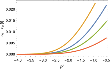
Figure 1: Dependence of the energy $\varepsilon_{n=0}$ on $\tilde{p}^{y}$ for a right-chiral electron in strong static magnetic field $B_{0}$, computed from Eq. (13). From top to bottom: $\Delta\phi_{\textsc{r}}^{-}=-2.3,-1.49,-0.7$, and $-0.2$. $p=p^{z}_{0}$, while the other parameters of the effective theory are the same as in Eq. (17). The states with $\tilde{p}^{y}\lesssim-3.5$ are completely localized within the bulk (Landau levels), the other states are localized at the boundary $x=-L_{\perp}/2$.

It follows from the above topological considerations that the support function $\rho_{n}(p)$ in Eq. (4) is non-vanishing as long as the momentum $p$ is inside the region of the one-dimensional projection of the Brillouin zone where the Chern number is finite (this region is approximately bounded by the positions of the two Weyl points). A significant part of this region lies outside the applicability range of the Weyl Hamiltonian, therefore there is no general reason to believe that the integral on the right-hand side of Eq. (4) can be calculated from the parameters of the effective low-energy theory. There still exists one noteworthy exception which is when the dispersion relation of Fermi arcs is separable, meaning that in the absence of magnetic field

$$\varepsilon_{0}(p,p^{y})=\mathcal{G}_{1}(p)+\mathcal{G}_{2}(p^{y}),$$ (14)

where $\mathcal{G}_{1,2}$ are some arbitrary functions. Here and below we choose the index $n=0$ for the branch of topologically non-trivial surface states. Indeed for $B_{0}=0$, the contribution of the surface states is insensitive to what happens outside the vicinity of the Weyl nodes. This is because according to Eq. (4), we get the integral of total derivative, which reduces to the difference of the boundary values of the function $\mathcal{G}_{1}$ at the points $p=p^{z}_{\textsc{wr}}$ and $p=p^{z}_{\textsc{wl}}$. These values themselves are fixed by the positions of the energies of the Weyl nodes $\varepsilon_{\textsc{wr}}$ and $\varepsilon_{\textsc{wl}}$, respectively, so that the partial contribution of the Fermi arc is

$$I^{\textsc{fa}}_{\text{surf}}(B_{0}=0)=\frac{e^{2}}{h^{2}c}B_{\textsc{AC}}S_{\perp}(\varepsilon_{\textsc{wr}}-\varepsilon_{\textsc{wl}}).$$ (15)

This is in agreement with Ref. Baireuther et al., 2016, where the contribution of these surface states to the total coefficient $\mathcal{C}_{\textsc{cme}}$ is argued to be equal to 1.

In case of non-vanishing $B_{0}$, the contribution to Eq. (4) beyond the effective theory remains unchanged, therefore the integral again reduces to the contribution from the states at the vicinity of the Weyl nodes. The latter is modified by the magnetic field albeit in a way that is completely defined by the low-energy effective theory. In order to specify Eq. (4) for this case, we note that within the effective theory, in the absence of the magnetic field, the energy of the Fermi arc is linear with respect to both $p$ and $p^{y}$ Witten (2015). It means that even in the case of $B_{0}\neq 0$, the separability holds both in the effective theory and in the ultraviolet complete theory, provided that the deviation from the Weyl node is large enough, $\delta p\gtrsim\Lambda_{0}$. Therefore, one can artificially split the integration region in Eq. (4) into two parts: the vicinities of the Weyl nodes, $\delta p\leq\Lambda$ ($\Lambda\gtrsim\Lambda_{0}$), and the rest. For the vicinities of the two Weyl nodes, we can still use the effective theory and we denote the result as $I_{\text{eff}}(\Lambda)$. Due to the linear dispersion, this contribution grows linearly with the cutoff $\Lambda$. In the remaining region, the separable relation (14) holds. The corresponding contribution is a linear function of $\Lambda$, which is equal to (15) at $\Lambda=0$, and its slope is opposite to that of $I_{\text{eff}}$. Since the total surface CME current is not sensitive to the choice of the cutoff $\Lambda$, we can formally set it to infinity:

$$I_{\text{surf}}=\lim\limits_{\Lambda\to\infty}\left(I_{\text{eff}}(\Lambda)-\Lambda\frac{dI_{\text{eff}}(\Lambda)}{d\Lambda}\right)+I^{\textsc{fa}}_{\text{surf}}(B_{0}=0).$$ (16)

For the actual calculation using Eq. (16) we have used the effective parameters of the bulk Hamiltonian

$$\varepsilon_{\textsc{wr}}=-\varepsilon_{\textsc{wl}}=4.9\times 10^{-2}t,\quad\varepsilon_{\textsc{f}}=0,$$ (17)

$$v^{z}=0.69t/\hbar,\quad v_{\perp}=2.0t/\hbar,\quad l_{\textsc{b}}=50,$$ (18)

and the two Weyl nodes share the same values of $v^{z}$ and $v_{\perp}$. Here $t$ is an arbitrary parameter that has dimension of energy. The specific choice of all these input parameters was done in order to compare them (see below) with the results of a particular microscopic calculation and with the results of Ref. Baireuther et al., 2016. We have found that even in the case of separable Fermi arcs, the resulting prefactor in (2) depends on the choice of $\Delta\phi$: for $\Delta\phi^{\pm}_{\textsc{r}}=-\Delta\phi^{\pm}_{\textsc{l}}=\pm 1.49$, $\mathcal{C}_{\textsc{cme}}=0.53$, while for $\Delta\phi^{\pm}_{\textsc{r}}=-\Delta\phi^{\pm}_{\textsc{l}}=\pm 2.3$, the result changes to $\mathcal{C}_{\textsc{cme}}=0.89$. (As before, the $+$ index corresponds to the boundary $x=L_{\perp}/2$, while the $-$ index corresponds to the other boundary.)

To conclude, the $\mathcal{C}_{\textsc{cme}}$ is not universal in the sense that it depends on both the bulk and the boundary parameters of the effective theory, even in the case of separable energy of Fermi arcs. As we have noted above, if the separability does not hold, the resulting current $I_{\text{surf}}$ involves microscopic details of the material beyond the information encoded in the parameters of the effective theory. Therefore, in order to understand whether the separability is a generic property of a WSM, in the following Section we study a microscopic model of such a material.

V Surface contribution in a microscopic theory

As we have established in the previous sections, the boundary CME is a significant effect, which under certain conditions dominates the longitudinal response of a WSM to the applied magnetic field. Although the Fermi arc states responsible for the effect are topologically protected, the magnitude of the boundary CME cannot be linked to any topological invariant. Moreover, the magnitude of the boundary CME is generally not fully determined by the parameters of the low-energy effective theory in the bulk material unless a special condition on the dispersion relation of the Fermi arc states is met. There is no obvious reason why this condition should hold for an arbitrary material interface therefore it is natural to assume that it is likely to be violated in a given experimental sample. Nevertheless, it is instructive to see how the condition breaks down in a particular microscopic model and what consequences this may have for the boundary CME.

To this end, we turn to the microscopic lattice Hamiltonian (6). The Bloch spectrum of the model contains one right-handed Weyl node located at $\bm{p}_{0}(\text{right})=(0,0,p^{z}_{\textsc{wr}})$, and one left-handed Weyl node located at $\bm{p}_{0}(\text{left})=-\bm{p}_{0}(\text{right}).$ The Bloch momentum $p^{z}_{\textsc{wr}}$ can be expressed in terms of the parameters of the Hamiltonian as described in Appendix A. By performing a unitary transformation from the original basis to the eigenbasis of the Hamiltonian at $\bm{p}=\bm{p}_{0}(\text{right})$, together with the linearisation with respect to $\bm{p}-\bm{p}_{0}(\text{right})$, the resulting effective Hamiltonian is

$$\mathcal{H}_{\text{R}}=\varepsilon_{\mathrm{diag}}(p^{z})\mathbb{1}_{2\times 2}+v_{\perp}(p^{x}\sigma^{x}+p^{y}\sigma^{y})+v^{z}(p^{z}-p^{z}_{\textsc{wr}})\sigma^{z}.$$ (19)

Here $\varepsilon_{\mathrm{diag}}(p^{z})=\varepsilon_{\textsc{wr}}+v_{\mathbb{1}}(p^{z}-p^{z}_{\textsc{wr}})$ and the relationships between the effective parameters and the parameters of the microscopic theory (6) are listed in Appendix A. The Hamiltonian (19) acts on the two-dimensional space which corresponds to the two gapless branches of the Hamiltonian’s Bloch spectrum near the Weyl point. The two remaining gapped branches have been dropped from the effective theory. Note that Eq. (19) has the same form as the effective Hamiltonian (1).

For the left-chiral node, a similar procedure leads to the same effective Hamiltonian (19), but with the replacement $(p^{z}_{\textsc{wr}},v^{z},\varepsilon_{\textsc{wr}})\to(-p^{z}_{\textsc{wr}},-v^{z},-\varepsilon_{\textsc{wr}})$. Note that the energies of the two Weyl nodes are equal in magnitude and have opposite signs, therefore the “symmetric” choice of the Fermi energy $\varepsilon_{\textsc{f}}=0$ results in equal density of oppositely charged carriers in the two Weyl pockets. For simplicity and in conformity with the reference study Baireuther et al., 2016, we limit our considerations to this symmetric situation.

For the actual numerical computations we have used one of the parameter sets from Ref. Baireuther et al., 2016, namely $\beta_{0}=0.1t$, $\beta^{z}=1.2t$, $M_{0}=-0.3t$, and $l_{\textsc{b}}=50$. By using the dictionary in Appendix A, one can see that this choice leads to the effective paramters listed in Eq. (17). The smallness of $\varepsilon_{\textsc{wr}}-\varepsilon_{\textsc{f}}$ ensures that the Fermi surfaces of the bulk states are close to the Weyl nodes, so that the effective theory describes the dynamics adequately. In addition, the parameter $v_{\mathbb{1}}^{z}$ turns out to be very small ($v_{\mathbb{1}}^{z}=-1.1\times 10^{-2}t/\hbar$), which results in accidental suppression of $I_{\text{bulk}}$ in a strong background field $B_{0}$ (see Sec. III).

We compute the energy spectrum of the bounded system, using the KWANT package Groth et al. (2014). This then serves as the input for the equation (4). Since we deal with a sample that is infinite in both $y$- and $z$-directions, we perform the dimensional reduction from three to one dimensions by replacing the operators $p$ and $p^{y}$ with corresponding good quantum numbers. We include the magnetic field by employing the standard Peierls substitution $\bm{p}\to\bm{p}-e\bm{A}/c$, and we choose the Landau gauge $\bm{A}=(0,Bx,0)$, which does not break the one-dimensional character of the problem. We have used 800 lattice sites in the $x$-direction, and checked that the doubling of this number does not change significantly any of the results presented below.

We have checked that the energy dispersion (11) for the Landau levels holds well and the deviations (beyond having non-zero $v_{\mathbb{1}}^{z}$) are in agreement with the dimensional analysis done in Appendix B.

We confirm that the boundary condition for the low-energy excitations that follows from the microscopic Hamiltonian (6) with the hard-wall boundaries indeed has the form (12). The extracted scattering phase-shifts turn out to be $\Delta\phi^{\pm}_{\textsc{r}}=-\Delta\phi^{\pm}_{\textsc{l}}=\pm 1.49$, which coincide with one of the two combinations that we used in Sec. IV. Futhermore, the numerical evaluation of the surface current (4) using KWANT gives the same value $\mathcal{C}_{\textsc{cme}}=0.53$ as we found in the effective theory. Surprisingly, we find that for the given set of parameters, the separability condition holds extremely well (within machine precision) in the microscopic theory, which explains the numerical agreement between the two results. Note that for the same set of parameters, the indicated value of the coefficient $\mathcal{C}_{\textsc{cme}}$ is close to the original finding $\mathcal{C}_{\textsc{cme}}\approx 1/2$ of Ref. Baireuther et al., 2016.

The next step is to see whether the result is robust against microscopic deformation of the boundary. We have modified the boundary by rescaling the $\beta_{0}$ parameter, $\beta_{0}\to 10\beta_{0}$, at the boundary sites of the 1D lattice. We have verified that such a modification does not affect the parameters of the bulk effective theory (19). At the same time, the phase-shifts changed significantly, $\Delta\phi^{\pm}_{\textsc{r}}=-\Delta\phi^{\pm}_{\textsc{l}}=\pm 2.3$. The resulting drastic change of the Fermi-arc dispersion is illustrated in Fig. 2. Apart from the quantitative modification of $\Delta\phi$, we have encountered a qualitative change: the separability condition for the Fermi arcs (Eq. (14)) is no longer satisfied. Thus, we conclude that the separability is rather an accidental property of the microscopic theory (6) with a specific boundary condition. The numerical diagonalisation for the modified boundary leads to $\mathcal{C}_{\textsc{cme}}=1.05$, which is quite different from the result for the original boundary. By recalling the result $\mathcal{C}_{\textsc{cme}}=0.89$ of the effective theory from Sec. IV (for the same phaseshifts $\pm 2.3$), we see that it is close to the finding within the microscopic theory, although the agreement between the two approaches is not that good anymore. This is a consequence of violating the separability condition and it makes the prediction of the effective theory unreliable.

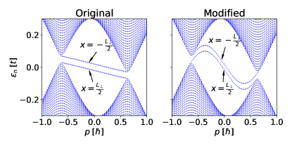
Figure 2: Energy spectrum for the original (left) and the modified boundaries (right) of the microscopic Hamiltonian (6). In both cases, surface states (Fermi arcs) form continuous lines connecting the Weyl nodes, but the shape of a given line is sensitive to the structure of the boundary. The parameters of the Hamiltonian are taken from Sec. V, $p^{y}=10^{-2}\hbar$, $B_{0}=0$. In order to illustrate the finite-size quantization of the energy bands, the number of lattice sites was decreased to 400.

VI Conclusion

In this paper, we have considered the adiabatic chiral magnetic effect (CME) in a WSM sample having a boundary. Generally, the contribution of the boundary to the CME current is on the same order as the bulk contribution, in particular both are proportional to the cross-sectional area of the sample. However we find that the boundary current can dominate in a presence of a strong static background magnetic field. This is true if the theory possesses a certain symmetry or if the parameters of the effective Hamiltonian are fine-tuned in a certain way, as is discussed in Sec. III.

We have found that there is no topological protection for such a boundary current and in general it cannot even be determined from the parameters of a bulk low energy effective theory. However, under a certain assumption (separability of the Fermi arc energy, Eq. (14)), the boundary current still can be expressed in terms of the parameters of the bulk effective theory alone (by which we mean the combination of the linearized Hamiltonian (1) and the boundary conditions (12)). Such an expression can be found in Eq. (16).

We have investigated the validity of the separability assumption in a particular microscopic model (6) used in Refs. Vazifeh and Franz, 2013 and Baireuther et al., 2016. This model accidentally has separable energy of the Fermi arcs, and the parameters of the Hamiltonian chosen in Ref. Baireuther et al., 2016 were so that the abovementioned fine-tuning takes place. This results in the surface current (16) being the only source for the adiabatic CME. However, we see that a deformation of the boundary layer in the model (6) both breaks the separability and makes Eq. (16) invalid. In conclusion, the adiabatic CME current in a bounded Weyl semimetal system is non-universal, but depends on the precise way one manufactures the boundaries of the sample.

Appendix A Relations between the parameters of the effective and the microscopic Hamiltonians

The effective parameters entering Eq. (19) are expressed via the original parameters of the microscopic Hamiltonian (6) as

$$v_{\perp}=2\sqrt{\frac{\beta_{z}^{2}-\beta_{0}^{2}}{\beta_{z}^{2}-4\varepsilon_{\textsc{wr}}^{2}}}$$ (20)

$$v_{\parallel}=\frac{\sqrt{\mathcal{K}}}{\beta_{z}^{2}-4\varepsilon_{\textsc{wr}}^{2}},$$ (21)

$$v_{\mathbb{1}}=-\frac{4\varepsilon_{\textsc{wr}}(1+M_{0})\sin p^{z}_{\textsc{wr}}+\beta_{0}\beta_{z}\cos p^{z}_{\textsc{wr}}}{\beta_{z}^{2}-4\varepsilon_{\textsc{wr}}^{2}},$$ (22)

where

$$\mathcal{K}=(4\varepsilon_{\textsc{wr}}(1+M_{0})\sin p^{z}_{\textsc{wr}}+\beta_{0}\beta_{z}\cos p^{z}_{\textsc{wr}})^{2}\\ +(\beta_{z}^{2}-4\varepsilon_{\textsc{wr}}^{2})(4(1+M_{0})^{2}\sin^{2}p^{z}_{\textsc{wr}}-\beta_{0}^{2}\cos^{2}p^{z}_{\textsc{wr}}).$$ (23)

Here, $p^{z}_{\textsc{wr}}$ is a positive solution of

$$\left(\frac{\beta_{0}}{\beta_{z}}\sin p^{z}_{\textsc{wr}}\right)^{2}+2(1+M_{0})\cos p^{z}_{\textsc{wr}}=2+2M_{0}+M_{0}^{2}-\frac{\beta_{z}^{2}-\beta_{0}^{2}}{4},$$ (24)

and the energy of right-chiral node is

$$\varepsilon_{\textsc{wr}}=-\frac{\beta_{0}}{\beta_{z}}\sin p^{z}_{\textsc{wr}}.$$ (25)

(For simplicity, we have set the hopping parameter equal to 1, $t=1$.)

Appendix B Higher-order corrections to the linearized effective Hamiltonian

By using the minimal effective Hamiltonian (1), we implicitly assume that the coupling to the magnetic field $B$ is captured completely by replacing the quasimomentum $\bm{p}=-i\hbar\bm{\nabla}$ with the operator $-i\hbar\bm{\nabla}-e\bm{A}/c$. However, since our particles have real spin $\bm{s}$ (as opposed to the pseudospin $\hbar\bm{\sigma}/2$), they are expected to have Zeeman coupling, which introduces the correction $\Delta\mathcal{H}_{\text{eff}}=-g\mu_{\textsc{b}}\bm{s}\bm{B}$, where $g$ is the $g$-factor and $\mu_{\textsc{b}}$ is the Bohr magneton. Then the energy gap between the two neighbouring Landau levels is of order of $v\hbar/l_{\textsc{b}}\sim e^{2}/l_{\textsc{b}}$, according to Eq. (11), while the corrections coming from the Zeeman coupling are expected to be suppressed by an additional factor $a_{\textsc{nn}}/l_{\textsc{b}}$, which is small for realistic fields $B\lesssim 10^{6}\;{\rm Gauss}\;$ that can be reached in laboratories in the foreseeable future. Here we have estimated the typical velocity $v$ of an electron and the crystalline lattice spacing $a_{\textsc{nn}}$ to be of order of the corresponding atomic units, $v\sim e^{2}/\hbar$, $a_{\textsc{nn}}\sim\hbar^{2}/m_{e}e^{2}$, which are not quite far from the results of the band-structure calculations for some WSMs Lee et al. (2015) and the direct X-ray diffraction measurements Boller and Parthé (1963); Xu et al. (2015). This irrelevance of Zeeman coupling is similar to what happens in graphene Goerbig (2011), although contrary to graphene, where the $g$-factor is not very far from the “bare” value $g=2$, see Ref. Zhang et al., 2006 we can have much larger $g$, which can in principle alter our conclusion. (In the estimate above, we assumed $g\sim 1$. For a similar discussion regarding the importance of the Zeeman coupling to WSMs, see Ref. Goswami et al., 2015.) Moreover, in materials with strong spin-orbit coupling such as the transition-metal monopnictides that were the first experimentally discovered WSMs Hasan et al. (2017), additional terms in the effective theory are allowed. One such term is $C_{b}\bm{B}\cdot\bm{b}$, where $\bm{b}=\bm{p}_{0}(\text{right})-\bm{p}_{0}(\text{left})$ is the momentum separation of the Weyl nodes. Also we neglect the higher-derivative corrections to the dispersion relation of a Weyl fermion, such as the quadratic term $\Delta\mathcal{H}_{\text{eff}}=C_{\text{2}}~{}(\bm{p}-\bm{p}_{0})^{2}/2m_{e}$, where $m_{e}$ is the “bare” electron mass. However, a similar kind of dimensional analysis reveals that in the absence of some “anomalously” large coupling constants $C_{b}$ and $C_{2}$, the resulting corrections are expected to be suppressed as well.

References

- Nielsen and Ninomiya (1983) H. B. Nielsen and M. Ninomiya, Physics Letters B 130, 389 (1983).
- Murakami (2007) S. Murakami, New Journal of Physics 9, 356 (2007).
- Wan et al. (2011) X. Wan, A. M. Turner, A. Vishwanath, and S. Y. Savrasov, Physical Review B 83, 205101 (2011).
- Xu et al. (2011) G. Xu, H. Weng, Z. Wang, X. Dai, and Z. Fang, Physical review letters 107, 186806 (2011).
- Burkov and Balents (2011) A. Burkov and L. Balents, Physical review letters 107, 127205 (2011).
- Weng et al. (2015) H. Weng, C. Fang, Z. Fang, B. A. Bernevig, and X. Dai, Physical Review X 5, 011029 (2015).
- Huang et al. (2015) S.-M. Huang, S.-Y. Xu, I. Belopolski, C.-C. Lee, G. Chang, B. Wang, N. Alidoust, G. Bian, M. Neupane, C. Zhang, et al., Nature communications 6 (2015).
- Xu et al. (2015) S.-Y. Xu, I. Belopolski, N. Alidoust, M. Neupane, G. Bian, C. Zhang, R. Sankar, G. Chang, Z. Yuan, C.-C. Lee, et al., Science 349, 613 (2015).
- Lv et al. (2015a) B. Lv, H. Weng, B. Fu, X. Wang, H. Miao, J. Ma, P. Richard, X. Huang, L. Zhao, G. Chen, et al., Physical Review X 5, 031013 (2015a).
- Lv et al. (2015b) B. Lv, N. Xu, H. Weng, J. Ma, P. Richard, X. Huang, L. Zhao, G. Chen, C. Matt, F. Bisti, et al., Nature Physics (2015b).
- Yang et al. (2015) L. Yang, Z. Liu, Y. Sun, H. Peng, H. Yang, T. Zhang, B. Zhou, Y. Zhang, Y. Guo, M. Rahn, et al., Nature physics 11, 728 (2015).
- Hasan et al. (2017) M. Z. Hasan, S.-Y. Xu, I. Belopolski, and S.-M. Huang, Annual Review of Condensed Matter Physics 8 (2017), 10.1146/annurev-conmatphys-031016-025225.
- Armitage et al. (2017) N. Armitage, E. Mele, and A. Vishwanath, (2017), http://arxiv.org/abs/1705.01111 .
- Vilenkin (1980) A. Vilenkin, Physical Review D 22, 3080 (1980).
- Fukushima et al. (2008) K. Fukushima, D. E. Kharzeev, and H. J. Warringa, Physical Review D 78, 074033 (2008).
- Kharzeev and Son (2011) D. E. Kharzeev and D. T. Son, Physical review letters 106, 062301 (2011).
- Kharzeev (2014) D. E. Kharzeev, Progress in Particle and Nuclear Physics 75, 133 (2014).
- Joyce and Shaposhnikov (1997) M. Joyce and M. Shaposhnikov, Physical Review Letters 79, 1193 (1997).
- Boyarsky et al. (2012a) A. Boyarsky, O. Ruchayskiy, and M. Shaposhnikov, Physical review letters 109, 111602 (2012a).
- Boyarsky et al. (2012b) A. Boyarsky, J. Fröhlich, and O. Ruchayskiy, Physical review letters 108, 031301 (2012b).
- Boyarsky et al. (2017) A. Boyarsky, A. Ivashko, and O. Ruchayskiy, in preparation (2017).
- Dvornikov and Semikoz (2015) M. Dvornikov and V. B. Semikoz, Physical Review D 91, 061301 (2015).
- Sigl and Leite (2016) G. Sigl and N. Leite, Journal of Cosmology and Astroparticle Physics 2016, 025 (2016).
- Boyarsky et al. (2015) A. Boyarsky, J. Fröhlich, and O. Ruchayskiy, Physical Review D 92, 043004 (2015).
- Vazifeh and Franz (2013) M. Vazifeh and M. Franz, Physical review letters 111, 027201 (2013).
- Yamamoto (2015) N. Yamamoto, Physical Review D 92, 085011 (2015).
- Adler (1969) S. L. Adler, Physical Review 177, 2426 (1969).
- Bell and Jackiw (1969) J. S. Bell and R. Jackiw, Il Nuovo Cimento A 60, 47 (1969).
- Son and Spivak (2013) D. Son and B. Spivak, Physical Review B 88, 104412 (2013).
- Burkov (2014) A. Burkov, Physical review letters 113, 247203 (2014).
- Li et al. (2016a) Q. Li, D. E. Kharzeev, C. Zhang, Y. Huang, I. Pletikosić, A. Fedorov, R. Zhong, J. Schneeloch, G. Gu, and T. Valla, Nature Physics (2016a), 10.1038/nphys3648.
- Zhang et al. (2016) C.-L. Zhang, S.-Y. Xu, I. Belopolski, Z. Yuan, Z. Lin, B. Tong, G. Bian, N. Alidoust, C.-C. Lee, S.-M. Huang, et al., Nature communications 7 (2016), 10.1038/ncomms10735.
- Dos Reis et al. (2016) R. Dos Reis, M. Ajeesh, N. Kumar, F. Arnold, C. Shekhar, M. Naumann, M. Schmidt, M. Nicklas, and E. Hassinger, New Journal of Physics 18, 085006 (2016).
- Schumann et al. (2017) T. Schumann, M. Goyal, D. A. Kealhofer, and S. Stemmer, arXiv preprint arXiv:1706.03172 (2017).
- Ganichev et al. (2001) S. Ganichev, H. Ketterl, W. Prettl, I. Merkulov, V. Perel, I. Yassievich, and A. Malyshev, Physical Review B 63, 201204 (2001).
- Wiedmann et al. (2016) S. Wiedmann, A. Jost, B. Fauqué, J. van Dijk, M. Meijer, T. Khouri, S. Pezzini, S. Grauer, S. Schreyeck, C. Brüne, et al., Physical Review B 94, 081302 (2016).
- Li et al. (2016b) Y. Li, Z. Wang, Y. Lu, X. Yang, Z. Shen, F. Sheng, C. Feng, Y. Zheng, and Z.-A. Xu, arXiv preprint arXiv:1603.04056 (2016b).
- Li et al. (2016c) Y. Li, L. Li, J. Wang, T. Wang, X. Xu, C. Xi, C. Cao, and J. Dai, Physical Review B 94, 121115 (2016c).
- Liang et al. (2016) T. Liang, S. Kushwaha, J. Kim, Q. Gibson, J. Lin, N. Kioussis, R. Cava, and N. Ong, arXiv preprint arXiv:1610.07565 (2016).
- Luo et al. (2016) Y. Luo, R. McDonald, P. Rosa, B. Scott, N. Wakeham, N. Ghimire, E. Bauer, J. Thompson, and F. Ronning, Scientific reports 6 (2016).
- Assaf et al. (2017) B. Assaf, T. Phuphachong, E. Kampert, V. Volobuev, G. Bauer, G. Springholz, L. de Vaulchier, and Y. Guldner, arXiv preprint arXiv:1704.02021 (2017).
- Chen et al. (2013) Y. Chen, S. Wu, and A. Burkov, Physical Review B 88, 125105 (2013).
- Goswami et al. (2015) P. Goswami, G. Sharma, and S. Tewari, Physical Review B 92, 161110 (2015).
- Chang and Yang (2015) M.-C. Chang and M.-F. Yang, Physical Review B 91, 115203 (2015).
- Ma and Pesin (2015) J. Ma and D. Pesin, Physical Review B 92, 235205 (2015).
- Zhong et al. (2016) S. Zhong, J. E. Moore, and I. Souza, Physical review letters 116, 077201 (2016).
- Alavirad and Sau (2016) Y. Alavirad and J. D. Sau, Physical Review B 94, 115160 (2016).
- Pesin (2016) D. Pesin, in Mathematical Methods in Electromagnetic Theory (MMET), 2016 IEEE International Conference on (IEEE, 2016) pp. 115–118.
- Baireuther et al. (2016) P. Baireuther, J. Hutasoit, J. Tworzydło, and C. Beenakker, New Journal of Physics 18, 045009 (2016).
- Ivashko and Cheianov (2017) A. Ivashko and V. Cheianov, (2017), https://arxiv.org/abs/1712.05613 .
- Note (1) We note that in Ref. \rev@citealpnumivashko2017adiabatic, the derivation was done for the geometry of a cylinder with a circular base. However, the generalization to the geometry of a slab is straightforward: one only needs to replace the momentum corresponding to the motion along the perimeter of the circle with the momentum , and to take into account that cylinder has only one boundary, while the slab has two. Additional factor in Eq. (4\@@italiccorr) is due to the fact that the inflow of the charge from the bulk to the boundary is splitted between the two boundaries. (For more details about the inflow mechanism, see Ref. \rev@citealpnumivashko2017adiabatic.).
- Johnson and Lippmann (1949) M. Johnson and B. Lippmann, Physical Review 76, 828 (1949).
- Berestetskii et al. (1982) V. B. Berestetskii, E. M. Lifshitz, and L. P. Pitaevskii, Quantum electrodynamics, Vol. 4 (Butterworth-Heinemann, 1982).
- Witten (2015) E. Witten, (2015), https://arxiv.org/abs/1510.07698 .
- Brown (1964) E. Brown, Physical Review 133, A1038 (1964).
- (56) “NIST Digital Library of Mathematical Functions,” http://dlmf.nist.gov/, f. W. J. Olver, A. B. Olde Daalhuis, D. W. Lozier, B. I. Schneider, R. F. Boisvert, C. W. Clark, B. R. Miller and B. V. Saunders, eds.
- Girvin (1999) S. M. Girvin, (1999), https://arxiv.org/abs/cond-mat/9907002 .
- Groth et al. (2014) C. W. Groth, M. Wimmer, A. R. Akhmerov, and X. Waintal, New Journal of Physics 16, 063065 (2014).
- Lee et al. (2015) C.-C. Lee, S.-Y. Xu, S.-M. Huang, D. S. Sanchez, I. Belopolski, G. Chang, G. Bian, N. Alidoust, H. Zheng, M. Neupane, et al., Physical Review B 92, 235104 (2015).
- Boller and Parthé (1963) H. Boller and E. Parthé, Acta Crystallographica 16, 1095 (1963).
- Goerbig (2011) M. Goerbig, Reviews of Modern Physics 83, 1193 (2011).
- Zhang et al. (2006) Y. Zhang, Z. Jiang, J. Small, M. Purewal, Y.-W. Tan, M. Fazlollahi, J. Chudow, J. Jaszczak, H. Stormer, and P. Kim, Physical review letters 96, 136806 (2006).