Intriguing Properties of Randomly Weighted Networks: Generalizing While Learning Next to Nothing

Abstract

Training deep neural networks results in strong learned representations that show good generalization capabilities. In most cases, training involves iterative modification of all weights inside the network via back-propagation. In Extreme Learning Machines, it has been suggested to set the first layer of a network to fixed random values instead of learning it. In this paper, we propose to take this approach a step further and fix almost all layers of a deep convolutional neural network, allowing only a small portion of the weights to be learned. As our experiments show, fixing even the majority of the parameters of the network often results in performance which is on par with the performance of learning all of them. The implications of this intriguing property of deep neural networks are discussed and we suggest ways to harness it to create more robust representations.

1 Introduction

Deep neural networks create powerful representations by successively transforming their inputs via multiple layers of computation. Much of their expressive power is attributed to their depth; theory shows that the complexity of the computed function grows exponentially with the depth of the net [1]. This renders deep networks more expressive than their shallower counterparts with the same number of parameters. Moreover, the data representation is more efficient from an information-theoretic point of view [2]. This has led to increasingly deeper network designs, some over a thousand layers deep [3].

Modern day architectures [4, 5, 3, 6] contain millions to billions of parameters [7] - often exceeding the number of training samples (typically ranging from tens of thousands [8] to millions [9]). This suggests that these networks could be prone to over-fitting, or are otherwise highly-overparameterized and could be much more compact; this is supported by network pruning methods, such as [10], which are able to retain network accuracy after removing many of the weights and re-training. Counter-intuitively, [11] have even shown that a network can be pruned by selecting an arbitrary subset of filters and still recover the original accuracy, hinting at a large redundancy in the parameter space. The large parameter space may explain why current methods in machine learning tend to be so data-hungry. Could be it that not all of the weights require updating, or are equally useful (this is suggested by [1])?

The common optimization pipeline involves an iterative gradient-based method (e.g. SGD), used to update all weights of the network to minimize some target loss function. Instead of training all weights, we suggest an almost extreme opposite: network weights are initialized randomly and only a certain fraction is updated by the optimization process. As our experiments show, while this does have a negative effect on network performance, its magnitude is surprisingly small with respect to the number of parameters not learned.

This effect holds for a range of architectures, conditions, and datasets, ruling out the option that it is specific to a peculiar combination thereof. We discuss and explore various ways of selecting subsets of networks parameters to be learned. To the best of our knowledge, while others have shown analytic properties of randomly weighted networks, we are the first to explore the effects of keeping most of the weights at their randomly initialized values in multiple layers. We claim that successfully training mostly-random networks has implications for the current understanding of deep learning, specifically:

1. Popular network architectures are grossly over-parameterized

2. Current attempts at interpreting emergent representations inside neural networks may be less meaningful than thought.

Moreover, he ability to do so opens up interesting possibilities, such as “overloading” networks by keeping a fixed backbone subset of parameters and re-training only a small set. This can be used to create cheap ensemble models which are nevertheless diverse enough to outperform a single model.

The rest of the paper is organized as follows. In Section 2 we describe related work. This is followed by a description of our method (Section 3), and an extensive set of experiments to limit the learned set of parameters in various ways. We end with some discussion and concluding remarks. For reproducibility, we will make code publicly available.

2 Related Work

Random Features

There is a long line of research revolving around the use of randomly drawn features in machine learning. Extreme Learning Machines show the utility of keeping some layer of a neural net fixed - but this is usually done only for one or two layers, and not within layers [12] or across multiple (more than two) layers. [13] has shown how picking random features has merits over matching kernels to the data. [14] have analytically shown useful properties of random nets with Gaussian weights. As mentioned in the work of [1], many of the theoretical works on deep neural networks assume specific conditions which are not known to hold in practice; we show empirically what happens when weights are selected randomly (and fixed) throughout various layer of the network and within layers.

Fixed Features

A very recent result is that of [15], showing - quite surprisingly - that using a fixed, Hadamard matrix [16] for a final classification layer does not hinder the performance of a classifier. In contrast, we do not impose any constraints on the values of any of the fixed weights (except drawing them from the same distribution as that of the learned ones), and evaluate the effect of fixing many different subsets of weights throughout the network.

Net Compression/Filter Pruning

Many works attempt to learn a compact representation by pruning unimportant filters: for example, compressing the network after learning [10, 17, 18, 11]; performing tensor-decompositions on the filter representations [19] or regularizing their structure to have a sparse representation [20]; and designing networks which are compact to begin with, either by architectural changes [21, 22], or by learning discrete weights , e.g. [23, 24].

Network Interpretability

There are many works attempting to dissect the representation learned within networks, in order to develop some intuition about their inner workings, improve them by “debugging” the representation or extract some meaningful explanation about the final output of the network. The work of [25] analyzes feature selectivity as network depth progresses. They also attempt to map the activities of specific filters back into pixel-space. Other methods mapping the output of the network to specific image regions has been suggested, either using gradient-based methods [26] or biologically inspired ones [27, 28]. Others either generate images that maximize the response of an image to a specific category [29]) or attempt to invert internal representations in order to recover the input image [30]. Another line of work, such as that of [31] shows how emergent representations relate to “interpretable” concepts. Some have tried to supervise the nets to become more interpretable [32]. The interpretability of a network is often defined by some correlation between a unit within the net and some concept with semantic meaning. As we keep most features random, we argue that (nearly) similarly powerful features can emerge without necessarily being interpretable. Admittedly, interpretability can be defined by examining a population of neurons, e.g. [33], but this kind of interpretation depends on some function which learns to map the outputs of a set of neurons to a given concept. In this regard, any supervised network is by construction interpretable.

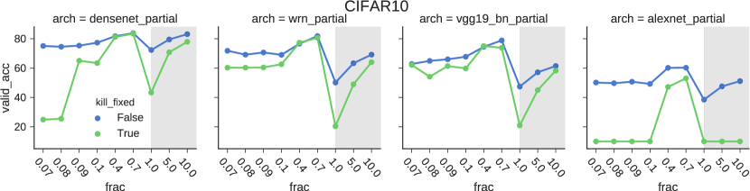
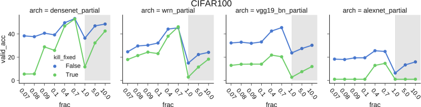
Figure 1: Training with only a few parameters (10 epochs): deep networks can generalize surprisingly well when only a small fraction of their parameters is learned. Y-axis is validation top-1% accuracy. Unshaded area specifies fraction of filters learned for at each convolutional layer. Shaded areas specify a fixed integer number of filters learned at each conv. layer. Blue lines represent training all except the specified frozen fraction. Green lines represent all but specified fraction of weights zeroed out.

3 Method: Learning Partial Networks

In standard settings, all weights of a neural network $N$ are learned in order to minimize some loss function $L$. Our goal is to test how many parameters actually have to be learned - and what effect fixing some of the parameters has on the final performance.

In this work we concern ourselves with vision-related tasks dealing with image classification, though in the future we intend to show it on non-vision (e.g, language) tasks as well. In this setting, the network is typically defined by a series of convolutional layers, interleaved by non-linearities (e.g, ReLU). The final layer is usually a fully-connected one, though it can be cast as a form of convolutional layer as well.

We proceed with some definitions. Let $\mathcal{W}$ be the set of all parameters of a network $N$. Assume $N$ has $n$ layers. All of our experiments can be framed as splitting $\mathcal{W}$ into two disjoint sets: $\mathcal{W}=\mathcal{W}_{f}\cup\mathcal{W}_{l}$. In each experiment we fix the weights of $\mathcal{W}_{f}$ and allow $\mathcal{W}_{l}$ to be updated by the optimizer. $\mathcal{W}_{f}$ are either randomly initialized or set to zero. $W_{l}=\cup_{i\in 1}^{n}w_{l,i}$ is a partition of $W_{l}$ into a selected set of weights $w_{l,i}$ for each layer $i\in\{1\dots n\}.$ Let $M_{i}\in\mathcal{R}^{O_{i}\times I_{i}\times k_{i}\times k_{i}}$ be the tensor defining the filters of layer $i$ of $N$, where: $O_{i}$ is the number of output channels (a.k.a number of filters), $I_{i}$ is the number of input channels, and $k_{i}$ is the kernel size.

For each convolutional layer, the corresponding $w_{l,i}$ defines a slice of some dimension of $M_{i}$:

• Slicing the first dimension this produces a subset of the filters, which will be learned: $f_{i,j}\subseteq\mathcal{F}{}_{i}$ where $\mathcal{F}{}_{i}$ is the set of filters of this layer.

• Slicing the second dimension, $w_{l,i}$ allows to learn only some of the incoming connections for each filter.

• Slicing the third and fourth dimensions $w_{l,i}$ allows to learn only some of the spatial locations of each filter.

We note that for layers with a bias term we do not split along any dimension other than the first. In addition, we keep fully-connected layers intact - we either learn them entirely or not at all.

For simplicity, we treat all filters in a homogeneous manner, e.g., no set of filters, such as “shortcut” filters used in resnets [6] is treated in a special way. In addition, selecting a subset of coefficients in some dimension is always implemented by choosing the first $p$ coefficients, where $p$ and the dimension depend on the specifics of the scenario we are currently testing. Admittedly, this could lead to suboptimal results (see below). However, the goal here is not to learn an optimal sparse set of connections (cf. [19, 20], but rather to show the power inherent in choosing an arbitrary subset of a given size.

Network training proceeds as usual, via back-propagation - only that the elements of $\mathcal{W}_{f}$ are treated as constants. We use Momentum-SGD with weight-decay for the optimization. Next, we describe various ways in to test how well the network converges to a solution for different configurations of $w_{l}$.

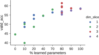
(a)

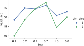
(b)

Figure 2: Training subsets of weights by slicing different dimensions of the weight tensor (densenet, one epoch) (a) fraction of total number of weights vs. selected dimension. dim_slice = 1: limiting output filters; 2: limiting input weights, 3,4: subsets of weights according to spatial location inside kernel. (b) fraction along selected dimension (<0) / size of slice along selected dimension (>=1) . Learning a subset of filters outperforms learning a subset of weights for each filter.

3.1 Splitting Network Parameters

As we cannot test all possible subsets of network parameters, we define a range of configurations to define some of them, as follows:

Fractional Layers: setting a constant fraction $p$ of filters of each layer $L$ of $N$, except the fully-connected (classification) layer. We do this for $p\in${$.07,.08,.09,.1,.4,.7\}$ (less than 0.07 will mean no filters for networks where $F_{0}=16$ e.g.., in WRN (wide resnets).

Integer number of filters: learning a constant integer $k\in\{1,5,10\}$ number of filters per layer. We show that learning a single filter in each layer leads to non-trivial performance for some architectures.

Single Layers: freezing all weights except those of a single block of layers. This is only for the wide and dense resnets. The blocks are selected as $\mathcal{W}_{l}\in\{conv_{1}block_{1},block_{2},block_{3},fc\}$ where $conv_{1}$ is the first convolutional layer, $block_{i}$ is one of 3 blocks of a wide-resnet with 28 layers and a widen factor of 4 or of a densenet with a depth of 100 and a growth-rate of 12.

Batch Normalization: we always use batch normalization layers if they are part of the original model. However, the BN layers also have optionally learnable parameters in addition to their running estimates of mean and variance. These are a multiplication $\gamma$ and bias term $\beta$ for each filter. Hence, the number of total weights in the BN layers amount to usually a few tens of thousands - dependent on the number of convolutional layers followed by BN layers and number of output channels for each. For example, in densenets this equals $\sim 24K$ parameters and $\sim 18K$ in WRN networks with a widen factor of 10.

Although BN layers are usually thought of as auxiliary layers to improve network convergence, we note that the benefits of learning the $\gamma,\beta$ parameters in a task dependent manner go beyond stabilization of the optimization process. This is exemplified by the work of [34] where the parameters of the BN layers are trained for each task. In our experiments, we take this a step further, to show what can be learned by tuning only the BN parameters of the network.

4 Experiments

We experiment with the CIFAR-10 and CIFAR-100 datasets [8] and several architectures: wide-residual networks, densely connected resnets, AlexNet, and VGG-19 (resp. [6, 35, 4, 5], as well as VGG-19 without batch-normalization (BN) [36]. For baselines, we modify a reference implementation. To evaluate many different configurations, we limit the number of training epochs for most of the experiments to 10 epochs (or even one epoch for some cases). In these cases, we also reduce the widening factor of the WRN to 4 from the default 10. For a few experiments we perform a full run (200 or 300 epochs, depending on network architecture).

All experiments were performed using an Ubuntu machine with a single Titan-X Pascal GPU, using the PyTorch deep-learning framework. Unless specified otherwise, models were optimized using Momentum-SGD.

4.1 Limiting Filter Inputs vs Outputs

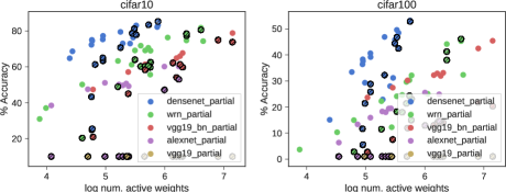
(a)

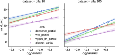
(b)

Figure 3: (a) Performance vs. absolute number of parameters (log scale), after training for 10 epochs. Much of the performance can be preserved by learning a relatively smaller no. of parameters, and even zeroing out the rest (thatched circles). densenet (blue) is very efficient in this sense, as it degrades most gradually with the decrease in the number of learned parameters. (b) fitting lines to performance vs. log fraction of learned parameters, this follows a logarithmic curve for various models.

As a first step, we establish in which dimension it is better to slice the filter tensor $M_{i}$ in each layer. Recall (Section 3) that learning a subset of the first dimension of $M_{i}$ translates to learning some of the filters but training all parameters for each filter (e.g., considering all inputs), while learning the second to fourth dimension means learning all filters but choosing some subset of the filter coefficients for each. Intuitively, allowing a subset of filters to be fully learned allows those learned filters to make full-use of the features in their incoming connections. On the other hand, learning all filters but selecting the same set of inputs for all of them to be fixed seems like a worse option, as this may cause important features to be “missed”; specifically, this can happen due to fixed bias term which cause the non-linearities to zero out the effect of these incoming features, rendering them “invisible” to subsequent layers.

We have tested this with the densenet [35] architecture on CIFAR-10, where we have sliced the convolutional layers along the four different dimensions and limited the number of epochs to just one. We tested this for a set fraction of each dimension, as well as a fixed-sized slice from each dimension, with a minimum of one element per slice. In Figure 2 (a) we plot the resulting performance vs the total number of parameters. For each dimension we set the minimal size of the selected slice to be 1. Because of this, slicing the third and fourth dimensions of $M_{i}$ results in a much larger number of learned parameters. In Figure 2 (b) we show results of learning slices of a given size along the first / second dimensions of $M_{i}$ for each layer.

Indeed, learning only a subset of the filters (dim_slice=1, blue) outperforms learning only a subset of the weights of each (dim_slice=2,green). As a result, all experiments hereafter will only demonstrate configurations involving subsets of filters (or entire layers).

4.2 Subsets of Filters

With the conclusion from the section above, we turn to experiment on various architectures and configurations, limiting ourselves to selecting a subset of filters, using the ways described in Section 3.1. We discuss the results below.

Figure 1 shows the top-1 accuracy after 10 training epochs. The best performer is densenets. AlexNet failed to learn for non-trivial fractions or for only a few filters per layer. Note the gap between the fixed weights and those zeroed-out. Zeroing out the weights effectively reduces the number of filters from the network. Using 70% of filters while zeroing the rest out achieves the same performance for densenets.

Shaded areas in Figure 1 specify learning a constant, integer number of filters at each layer. Interestingly, learning only a single filter per layer can result in a non-trivial accuracy. In fact, zeroing out all non-learned weight, resulting in a net with a single-filter per layer, still is able to do much above chance, around 45% on CIFAR-10 with resnets. VGG-19 without the BN layers failed to converge to performance better than chance for any of these settings.

Parameter Efficiency

Another view on the results can be seen in Figure 3 (a) which plots the performance obtained vs. the total number of parameters on a logarithmic scale. Even when zeroing out all non-learned parameters (thatched circles), densenets attain decent performance with less that 100K parameters, roughly an eighth of the original amount. We fit a straight line to the performance vs. the log of the fraction of learned parameters (Figure 3 (b)). The performance grows logarithmically with the number of parameters, with a larger slope (e.g., better utilization of added parameters for recent architectures (resnet, WRN).

Subsets of Layers

We learn only subsets of layers out of the layers specified and report the performance for each of these scenarios, for CIFAR-10 and CIFAR-100 and for the dense and wide residual networks. Table 4.2 summarizes this experiment. We see that a non-trivial accuracy can be reached by learning only a single of the layer subsets. Furthermore, in most cases learning the last, fully-connected layer on its own proves inferior to doing so with another layer. For example, with wide-resnets (WRN) learning the fc (fully connected) layer attains only 37% top-1 accuracy on CIFAR-10, much less than either than the 3 middle blocks. While the number of parameters in fc is indeed much lower, note that it grows linearly with the number of classes while that of the middle blocks remains constant (this is not seen directly in the table due to the additional weights of BN layers learned). From a practical point of view, this can indicate that when fine-tuning a single layer of a network towards a new task, the last layer is not necessarily the best one to choose. Nevertheless, fine-tuning an additional layer in the middle can prove useful as the additional parameter cost can be quite modest.

arch	Params	layer	Eff. Params	C10	C100
densenet	0.77- 0.8M	BN	24K	60.85	16.06
		$conv_{1}$	24.6K	64.76	15.08
		$block_{1}$	194K	73.02	22.89
		$block_{2}$	259K	72.95	28.00
		$block_{3}$	291K	76.33	31.18
		$fc$	27.4K / 58.3K	68.63	33.43
WRN	5.85- 5.87M	BN	7.2K	30.2	3.76
		$conv_{1}$	7.63K	30.93	3.67
		$block_{1}$	275K	61.19	12.23
		$block_{2}$	1.12M	76.32	25.07
		$block_{3}$	4.46M	74.31	32.35
		$fc$	9.77K / 32.9K	37.03	10.31

Table 1: Learning only a subset of layers (10 epochs): learning only the fully-connected layer usually proves inferior to learning one of the middle blocks (see $fc$ vs. $block_{i},i\in\{1,2,3\}$). Learning only the batch-norm (BN) layer results in non-trivial performance. Params: total parameters. Eff. Params: number of learned parameters. WRN: Wide-residual Networks.

Batch-Norm Layers

As mentioned in Section. 3.1 we tested network performance when learning only batch-normalization layers. This experiment was done for the wide and dense residual network. Learning only the parameters of the BN layers can in non-trivial performance using densenets, e.g. 60.85% for CIFAR-10 (vs 68.6 for BN+fc) and 30.2. For CIFAR-100 this is no longer the case, 16% vs 33.4%. Please refer to Table 4.2.

In addition, we compare the performance for various learned network fractions when batch-norm is turned on and off for WRN and densenets. This is summarized in Figure 4. We can see that when a small fraction of parameters ($\leq 0.1$, or a constant integer number of filters per layer) is used, BN layers make a big difference. However, starting from $0.4$ the difference becomes smaller. This is likely because the representative power introduced by the BN parameters becomes less significant as more parameters are introduced (i.e., learned by the optimizer).

In this figure, we also see the performance attainable by training 100% of the weights for each architecture (black dashed lines). Notably, using 70% percent of parameters induces little or no loss in accuracy - and for densenet, we can achieve the full-accuracy with 10 filters per layer. From this we see that there are various ways to distribute the fraction of parameters trained in the network to achieve similar accuracies.

Achieving high accuracy with as much as 40% filters learned is also consistent with the result we got on the full training runs (see below).

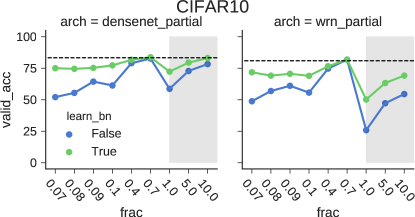
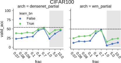
Figure 4: Learning different fractions of a network (10 epochs), with and without batch-norm layers. Batch-normalization accounts for much of the accuracy when the number of weights is reduced but become less significant when using a large (>40%) fraction of weights. Black dashed lines are for using all-weights with batch-norm.

Full Runs

We also ran full training sessions for WRN and densenet (200,300 epochs respectively) with a limited no. of parameters on CIFAR-10. Specifically, WRN , when 60% of the filters are arbitrarily zeroed out, achieve almost the baseline performance of 96.2%. Please refer to Table 2 for numerical results of this experiment. We note that when learning a single filter for each layer, densenets outperform WRN by a large gap, 85% vs 69% on CIFAR-10 and 59.7% vs 34.85 on CIFAR-100.

On CIFAR-100, the gap between the accuracy attained with a fraction of parameters vs all of them is larger when using a few parameter than on CIFAR-10. This is visualized in Figure 5.

Method	Fraction	Eff. Params $\times 10^{6}$	Perf	Perf$\dagger$
WRN	0.1	3.66	94.12	91.53
WRN	0.4	14.6	95.75	95.49
densenets	0.1	0.09	88.73	82.11
densenets	0.4	0.3	93.33	92.46

Table 2: Performance vs fraction of parameters learned on CIFAR-10 (full training, 200/300 epochs). $\dagger$ means performance when $w_{f}$ (fixed parameters) are all set to zero. Eff. Params means number of params updated in learning.

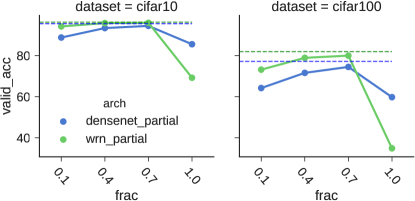
Figure 5: Learning only a fraction of weights, full runs: learning CIFAR-10 can be done effectively when most of the weights are fixed at their random initialized state(left). For CIFAR-100 a larger portion of parameters is needed (right). Green and blue dashed lines represent results with all weight learned for WRN, densenets respectively.

Tiny-ImageNet

% Params	Top-1 Accuracy %	# Params
10	21.75	.83M
40	30.13	2.58M
70	33.22	4.33M
100	35.54	6.1M

Table 3: Training partial models on the Tiny-ImageNet dataset.

Finally, we perform a larger scale experiment. We choose the Tiny-ImageNet . This dataset is a variant of the larger ImageNet [9] dataset. It contains two-hundred image categories, with 500 training and 50 validation images for each. The images are downscaled to 64x64 pixels. In this experiment we use the recent YellowFin optimizer [37] for which we found there is less need for manual tuning than SGD. We train for a total 45 epochs, with an initial learning rate of 0.1, which is lowered by a factor of 10 after 15 and after 30 iterations. We use the WRN architecture with a widen-factor of 4. The same architecture was shown to perform quite reasonably well on another downs-scaled version of ImageNet in [34]. We train the fully-parameterized version, and partial versions with fractions of 0.1,0.4 and 0.7 of the filters in each conv. layer.

The results of this experiment are summarized in Table 3. The value of the fully-parameterized version (last row in the table) is of little importance. Note how with 70% of the parameters trained, we lose %2.3 in the top-1 accuracy, and another 3.1% for 40% of the convolutional layers.

4.3 Cheap Ensembles

Training a network while keeping most weights fixed enables the creation of “cheap” ensemble models that share many weights and vary only the remaining portion. For example, training a densenet model while learning only 10% of the weights requires roughly 90K new parameters for each such model. The total cost for e.g., an ensemble model of size 5 will be $.77+09*4=1.13M$ parameters, much less than training five independent models. But will the resulting ensemble be as diverse as five independently trained models? Using densenets and testing on CIFAR-10, we trained three ensemble models of 5 elements each. We first train a fully-parametrized model for one epoch and use it as a starting point to train each ensemble element for an additional epoch. In this experiment, we tried both the Adam [38] Optimizer and SGD and reported for each ensemble type the best of the two results.

We report for each ensemble the mean accuracy of elements, the accuracy attained averaging the ensemble’s predictions and the total number of learned parameters (except of the first fully-parametrized model). We trained ensembles of (a) fully parameterized models (Full) (b) models varying only by the fc layer (FC) and (c) models with a shared fraction $R$ of convolutional weights (Share-Conv-R). Table 4 summarizes the results. We see that fixing 10% (sharing 90%) of the parameters already outperforms re-training only the FC layers. A fully-parameterized ensemble indeed shows better variability in the solutions (leading to a better ensemble performance), though using some portion of shared conv. weights is not far below it, with significantly less weights.

Model Type	No. Params	Mean Accuracy	Ensemble Accuracy
FC	137K	68.5	70.25
Share-Conv-0.9	451K	69.9	71.14
Share-Conv-0.6	1.53M	71	73.54
Share-Conv-0.3	2.66M	71.3	75.47
Full	3.85M	71.7	76.35

Table 4: Ensemble models. Ensemble models with some convolutional weight sharing between elements perform similarly to independently trained models though being significantly more compact. Relearning some of the conv. weights

4.4 Weight Magnitudes

We perform an analysis of the magnitude distribution of the weights within learned vs. fixed layers. This is motivated by the observation that relatively small weights can lead to better generalization bounds [39, 40]. We analyze the magnitudes of the weights of the convolutional layers of the experiment in the above Section 4.2 (on the Tiny-ImageNet dataset). For each convolutional layer, we record the mean of the absolute weight value and the variance of the weights. For layers with fixed weights, we report this value as well. The mean and variance of the fixed weights is determined by the random initialization.

We plot the results in Figure 6. The magnitudes of training only 10% of the convolutional weights stand out as being relatively high. For training 40%, 70% and 100% (all weights), the magnitudes seem to be distributed quite similarly, with 70% and 100% being nearly indistinguishable. If the average magnitude of weights is indeed any indication of the generalization capacity of the network, in this context it seems to be consistent with the rest of our findings, specifically the performance of the partially trained nets as seen in Table 3.

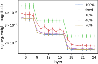
Figure 6: Weight distribution across convolutional layers as a function of the percentage of learned convolutional weights. The mean value of any fraction above 40% of trained parameters is stable and similar to that of a fully-trained network. “Fixed” is simply the distribution of randomly-initialized weights.

5 Discussion

We have demonstrated that learning only a small subset of the parameters of the network or a subset of the layers leads to an unexpectedly small decrease in performance (with respect to full learning) - even though the remaining parameters are either fixed or zeroed out. This is contrary to common practice of training all network weights. We hypothesize this shows how over-parameterized current models are, even those with a relatively small number of parameters, such as densenets. We have tested a large number of configurations of ways to limit the subsets of learned network weights. This choice of subset has a large impact on the performance of the resulting network. Some network architectures are more robust to fixing most of their weights than others. Learning is also possible with an extremely small number of filters learned at the convolutional layers, as little as a single filter for each of these layers. Three simple applications of the described phenomena are (1) cheap ensemble models, all with the same “backbone” fixed network, (2) learning multiple representations with a small number of parameters added to each new task and (3) transfer-learning (or simply learning) by learning a middle layer vs the final classification layer. We intend to explore these directions in future work, as well as testing the reported phenomena on additional, non-vision related tasks, such as natural language processing or reinforcement-learning.

References

- [1] M. Raghu, B. Poole, J. Kleinberg, S. Ganguli, and J. Sohl-Dickstein, “On the expressive power of deep neural networks,” arXiv preprint arXiv:1606.05336, 2016.
- [2] R. Shwartz-Ziv and N. Tishby, “Opening the Black Box of Deep Neural Networks via Information,” arXiv preprint arXiv:1703.00810, 2017.
- [3] K. He, X. Zhang, S. Ren, and J. Sun, “Identity mappings in deep residual networks,” in European Conference on Computer Vision. Springer, 2016, pp. 630–645.
- [4] A. Krizhevsky, I. Sutskever, and G. E. Hinton, “Imagenet classification with deep convolutional neural networks,” in Advances in neural information processing systems, 2012, pp. 1097–1105.
- [5] K. Simonyan and A. Zisserman, “Very deep convolutional networks for large-scale image recognition,” arXiv preprint arXiv:1409.1556, 2014.
- [6] S. Zagoruyko and N. Komodakis, “Wide Residual Networks.” CoRR, vol. abs/1605.07146, 2016.
- [7] N. Shazeer, A. Mirhoseini, K. Maziarz, A. Davis, Q. Le, G. Hinton, and J. Dean, “Outrageously large neural networks: The sparsely-gated mixture-of-experts layer,” arXiv preprint arXiv:1701.06538, 2017.
- [8] A. Krizhevsky and G. Hinton, “Learning multiple layers of features from tiny images,” 2009.
- [9] O. Russakovsky, J. Deng, H. Su, J. Krause, S. Satheesh, S. Ma, Z. Huang, A. Karpathy, A. Khosla, M. Bernstein et al., “Imagenet large scale visual recognition challenge,” International Journal of Computer Vision, vol. 115, no. 3, pp. 211–252, 2015.
- [10] H. Li, A. Kadav, I. Durdanovic, H. Samet, and H. P. Graf, “Pruning filters for efficient convnets,” arXiv preprint arXiv:1608.08710, 2016.
- [11] D. Mittal, S. Bhardwaj, M. M. Khapra, and B. Ravindran, “Recovering from Random Pruning: On the Plasticity of Deep Convolutional Neural Networks,” 2018.
- [12] G. Huang, G.-B. Huang, S. Song, and K. You, “Trends in extreme learning machines: A review,” Neural Networks, vol. 61, pp. 32–48, 2015.
- [13] A. Rudi and L. Rosasco, “Generalization properties of learning with random features,” in Advances in Neural Information Processing Systems, 2017, pp. 3218–3228.
- [14] R. Giryes, G. Sapiro, and A. M. Bronstein, “Deep Neural Networks with Random Gaussian Weights: A Universal Classification Strategy?” arXiv preprint arXiv:1504.08291, 2015.
- [15] E. Hoffer, I. Hubara, and D. Soudry, “Fix your classifier: the marginal value of training the last weight layer,” arXiv preprint arXiv:1801.04540, 2018.
- [16] K. J. Horadam, Hadamard matrices and their applications. Princeton university press, 2012.
- [17] S. Han, H. Mao, and W. J. Dally, “Deep compression: Compressing deep neural networks with pruning, trained quantization and huffman coding,” arXiv preprint arXiv:1510.00149, 2015.
- [18] S. Han, J. Pool, J. Tran, and W. Dally, “Learning both weights and connections for efficient neural network,” in Advances in Neural Information Processing Systems, 2015, pp. 1135–1143.
- [19] B. Liu, M. Wang, H. Foroosh, M. Tappen, and M. Pensky, “Sparse convolutional neural networks,” in Proceedings of the IEEE Conference on Computer Vision and Pattern Recognition, 2015, pp. 806–814.
- [20] W. Wen, C. Wu, Y. Wang, Y. Chen, and H. Li, “Learning structured sparsity in deep neural networks,” in Advances in Neural Information Processing Systems, 2016, pp. 2074–2082.
- [21] F. N. Iandola, S. Han, M. W. Moskewicz, K. Ashraf, W. J. Dally, and K. Keutzer, “SqueezeNet: AlexNet-level accuracy with 50x fewer parameters and¡ 0.5 MB model size,” arXiv preprint arXiv:1602.07360, 2016.
- [22] A. G. Howard, M. Zhu, B. Chen, D. Kalenichenko, W. Wang, T. Weyand, M. Andreetto, and H. Adam, “Mobilenets: Efficient convolutional neural networks for mobile vision applications,” arXiv preprint arXiv:1704.04861, 2017.
- [23] O. Shayar, D. Levi, and E. Fetaya, “Learning Discrete Weights Using the Local Reparameterization Trick,” arXiv preprint arXiv:1710.07739, 2017.
- [24] M. Rastegari, V. Ordonez, J. Redmon, and A. Farhadi, “Xnor-net: Imagenet classification using binary convolutional neural networks,” in European Conference on Computer Vision. Springer, 2016, pp. 525–542.
- [25] M. D. Zeiler and R. Fergus, “Visualizing and understanding convolutional networks,” in European conference on computer vision. Springer, 2014, pp. 818–833.
- [26] B. Zhou, A. Khosla, A. Lapedriza, A. Oliva, and A. Torralba, “Learning deep features for discriminative localization,” in Computer Vision and Pattern Recognition (CVPR), 2016 IEEE Conference on. IEEE, 2016, pp. 2921–2929.
- [27] M. Biparva and J. Tsotsos, “STNet: Selective Tuning of Convolutional Networks for Object Localization,” in The IEEE International Conference on Computer Vision (ICCV), vol. 2, 2017.
- [28] J. Zhang, Z. Lin, J. Brandt, X. Shen, and S. Sclaroff, “Top-down neural attention by excitation backprop,” in European Conference on Computer Vision. Springer, 2016, pp. 543–559.
- [29] K. Simonyan, A. Vedaldi, and A. Zisserman, “Deep inside convolutional networks: Visualising image classification models and saliency maps,” arXiv preprint arXiv:1312.6034, 2013.
- [30] A. Mahendran and A. Vedaldi, “Understanding deep image representations by inverting them,” in Computer Vision and Pattern Recognition (CVPR), 2015 IEEE Conference on. IEEE, 2015, pp. 5188–5196.
- [31] D. Bau, B. Zhou, A. Khosla, A. Oliva, and A. Torralba, “Network Dissection: Quantifying Interpretability of Deep Visual Representations,” arXiv preprint arXiv:1704.05796, 2017.
- [32] Y. Dong, H. Su, J. Zhu, and F. Bao, “Towards interpretable deep neural networks by leveraging adversarial examples,” arXiv preprint arXiv:1708.05493, 2017.
- [33] R. Fong and A. Vedaldi, “Net2Vec: Quantifying and Explaining how Concepts are Encoded by Filters in Deep Neural Networks,” arXiv preprint arXiv:1801.03454, 2018.
- [34] S.-A. Rebuffi, H. Bilen, and A. Vedaldi, “Learning multiple visual domains with residual adapters,” arXiv preprint arXiv:1705.08045, 2017.
- [35] G. Huang, Z. Liu, K. Q. Weinberger, and L. van der Maaten, “Densely connected convolutional networks,” arXiv preprint arXiv:1608.06993, 2016.
- [36] S. Ioffe and C. Szegedy, “Batch normalization: Accelerating deep network training by reducing internal covariate shift,” in International Conference on Machine Learning, 2015, pp. 448–456.
- [37] J. Zhang, I. Mitliagkas, and C. Ré, “YellowFin and the Art of Momentum Tuning,” arXiv preprint arXiv:1706.03471, 2017.
- [38] D. Kingma and J. Ba, “Adam: A method for stochastic optimization,” arXiv preprint arXiv:1412.6980, 2014.
- [39] P. L. Bartlett, “For valid generalization the size of the weights is more important than the size of the network,” in Advances in neural information processing systems, 1997, pp. 134–140.
- [40] P. Zhou and J. Feng, “The Landscape of Deep Learning Algorithms,” arXiv preprint arXiv:1705.07038, 2017.