Entropic bounds between two thermal equilibrium states

Abstract

The positivity conditions of the relative entropy between two thermal equilibrium states $\hat{\rho}_{1}$ and $\hat{\rho}_{2}$ are used to obtain upper and lower bounds for the subtraction of their entropies, the Helmholtz potential and the Gibbs potential of the two systems. These limits are expressed in terms of the mean values of the Hamiltonians, number operator, and temperature of the different systems. In particular, we discuss these limits for molecules which can be represented in terms of the Franck–Condon coefficients. We emphasize the case where the Hamiltonians belong to the same system at two different times $t$ and $t^{\prime}$. Finally, these bounds are obtained for a general qubit system and for the harmonic oscillator with a time dependent frequency at two different times.

I Introduction

The states of quantum systems are described either by vectors $|\psi\rangle$ in a Hilbert space ${\cal H}$ Dirac-book (pure states) and the corresponding wave functions $\psi(x)=\langle x|\psi\rangle$ Schroed1926 ; *Schroed19261 or by the density operators $\hat{\rho}$ acting in the Hilbert space Landau27 ; vonNeumann27 (mixed states). These states are associated to Hamiltonian system interactions with certain environments or external sources. The systems can consist of a constant number of particles or, due to the interactions, can have a varying number of particles. In view of this, there are mixed states with density operators in equilibrium, depending on such physical parameters as the temperatures and chemical potentials.

In quantum mechanics, one can find various characteristics of arbitrary pure and mixed states in terms of the von Neumann vonNeumannbook , Tsallis Tsallis , and Rényi entropies Renyi , as well as known equalities and inequalities; see, for example, Lieb ; *Lieb2; Ruskai ; *Ruskaie; Araki . On the other hand, the correlations of a system with an external source can be of such a form that it preserves the purity of the states but the system Hamiltonian depends on time; this means that the system energy changes due to the interchange with the external source, and this change is described by the time dependence of the Hamiltonian parameters.

The variations of the parameters may be either very slow or very fast with respect to the relaxation time of the system. In the case of a very fast change in the Hamiltonian parameters (instantaneous rate of change), the studied state, being either pure or mixed, just after the perturbation continues to be the same as it was before due to inertia. Thus, if the system was in the pure state with a given energy level, the wave function just after the perturbation does not change in spite of the fact that the Hamiltonian is modified. Similarly if the system was in a thermal equilibrium mixed state with the density operator $\hat{\rho}$, this operator is the same just after the instant Hamiltonian parameter variation, though the Hamiltonian itself is different.

Our generic approach is to study the bounds for the state characteristics making use of the relative entropy between two thermal states, concentrating the applications of the inequalities to the thermal equilibrium states and their possible changes. This is related to the developments of the studies of states associated with quantum thermodynamics. In fact, in recent years the analysis of the thermodynamic properties of the information (quantum and classical) has been the subject of several works huber ; parrondo ; maruyama ; esposito ; brandao ; skrzypczyk ; faist ; strasberg ; campisi ; mancino . In particular, the fundamental thermodynamical aspects of information as the second law, the Landauer principle and the Maxwell’s demon have been studied plenio ; maruyama ; esposito . In relation with the fundamental aspects of statistical mechanics, we stress that in Popescu2006 a general canonical principle has been proposed without using temporal or ensemble averages, which however can be easily connected to the standard statistical mechanics. How entanglement and coherence can be used to generate work has been the subject of Brandao2008 ; funo13 ; ren ; korzekwa16 . The problem of how the thermodynamic quantities as the internal energy, the entropy, and the Helmholtz potential behave as a system approach equilibrium has been of interest. These investigations have led to the definition of different inequalities regarding these quantities esposito ; figueroa ; julio .

In the previous works figueroa ; julio , we have analyzed the comparison between an arbitrary state with the density matrix $\hat{\rho}$ and a thermal equilibrium state $\hat{\sigma}=e^{-\hat{H}/T}/{\rm Tr}(e^{-\hat{H}/T})$ making use of the Tsallis and von Neumann relative entropies. This comparison was made in specific for a qubit system and a Gaussian state resulting in an inequality that relates the entropy of $\hat{\rho}$, the mean value ${\rm Tr}(\hat{\rho}\hat{H})$, and the partition function of the system $Z(\hat{H},T)={\rm Tr}(e^{-\hat{H}/T})$. The bounds for physical characteristics as the energy or entropy of quantum states play an important role since they determine the specific states which correspond on the extreme situation where the equality between the bound an the physical quantity of interest are equal. In our work figueroa it was shown that the distance, given the relative entropy expression, between the arbitrary state with density matrix $\hat{\rho}$ and the canonical thermal equilibrium state with Hamiltonian $\hat{H}$ provides the bound for the sum of the energy and the entropy (in dimensionless variables). Exactly on this bound the canonical Boltzmanian density matrix is realized as it was point out also in nouvo . The observation that the physical state of thermal equilibrium is related with the bound gives the motivation to study other bounds in quantum thermodynamics. In this work we study, using the relative entropy as a distance between the quantum states, the bounds for differences of entropies and free energies associated with states corresponding to different Hamiltonians and temperatures. Such bounds give the possibility to study the specific states which appear when the Hamiltonians depend on time. Specifically we are interested in how the system behaves when a sudden change in these parameters is done. Such situation takes place if the duration of the parameter change is smaller than the relaxation time of the system, e.g., in molecular spectroscopy such regime is associated with the Franck-Condon factors which are used to describe the vibronic structure of electronic lines in molecules if the transition takes place between the pure energy level states. We point out that the results from this research can be of importance in the field of quantum information thermodynamics.

In this work, we obtain new upper and lower limits of the difference of the entropy, the Helmholtz and Gibbs potentials between two different thermal equilibrium density matrices $\hat{\rho}_{1}$ and $\hat{\rho}_{2}$. Although these two states can be not related, we make special emphasis in the case where they describe the same system at two different times $t$ and $t^{\prime}$. As, in principle, the initial and final states may not have the same purity, one can think that the initial state with number operator $\hat{N}_{1}$ is in contact with an external source at temperature $T_{1}$, whose interaction yields an effective Hamiltonian $\hat{H}_{1}$ over the system. At some point, a change in the interaction $\hat{H}_{1}\rightarrow\hat{H}_{2}$, the number operator $\hat{N}_{1}\rightarrow\hat{N}_{2}$, and the temperatures $T_{1}\rightarrow T_{2}$ is done by the energy or particle transfer between the system and the external source, changing the thermodynamic properties of the system. It is important to stress that the expressions obtained can be applied to any type of change done to the system, i.e., if these changes are either quasistatic or not.

As examples, these bounds are studied for a general qubit system and the harmonic oscillator with a time-dependent frequency.

II Bounds between two systems interchanging energy

First, we discuss the case where the system is represented by the Hamiltonian $\hat{H}$ and the parameter $T$, and may interact with an external source only through energy exchanges. As it is known, the description of such a system can be done using the canonical ensemble. In this representation, any state given by the density operator $\hat{\sigma}=e^{-\hat{H}/T}/{\rm Tr}(e^{-\hat{H}/T})$ has the von Neumann entropy $S=-{\rm Tr}(\hat{\sigma}\ln\hat{\sigma})$. This entropy can also be expressed as $S=\langle\hat{H}\rangle/T+\ln Z(\hat{H},T)$, where the quantity $Z(\hat{H},T)={\rm Tr}(e^{-\hat{H}/T})$ is called the partition function while the parameter $T$ is the temperature. In this case, the operator $\hat{\sigma}$ describes a thermal equilibrium state (in a unit system where $\hbar=k=1$).

As we compare an arbitrary nonthermal equilibrium state $\hat{\rho}$ with $\hat{\sigma}$ using the nonnegative relative entropy nielsen ${\rm Tr}(\hat{\rho}(\ln\hat{\rho}-\ln\hat{\sigma}))$, one can notice that the entropy of the nonequilibrium system must satisfy the inequality $S<{\rm Tr}\,(\hat{\rho}\hat{H})/T+\ln Z(\hat{H},T)$, which can be used to distinguish the equilibrium state from the nonequilibrium one figueroa ; julio . Also, we point out that another inequality can be defined when the operator $\hat{H}$ and the temperature $T$ are replaced by an arbitrary observable $\hat{\mathcal{O}}$ and parameter $\lambda$, respectively, i.e., by doing the replacement $\hat{\sigma}\rightarrow e^{-\hat{\mathcal{O}}/\lambda}/{\rm Tr}(e^{-\hat{\mathcal{O}}/\lambda})$. Later on this idea will be used to find bounds for a grand canonical ensemble.

We consider two thermal equilibrium states described by the Hamiltonians and temperatures (or arbitrary parameters) ($\hat{H}_{1}$, $T_{1}$) and ($\hat{H}_{2}$, $T_{2}$), respectively,

$$\hat{\rho}_{1}=\frac{e^{-\beta_{1}\hat{H}_{1}}}{\textrm{Tr}\,(e^{-\beta_{1}\hat{H}_{1}})},\quad\hat{\rho}_{2}=\frac{e^{-\beta_{2}\hat{H}_{2}}}{\textrm{Tr}(e^{-\beta_{2}\hat{H}_{2}})}\,,$$ (1)

with $\beta_{1}=1/T_{1}$ and $\beta_{2}=1/T_{2}$. The difference of their entropies is given by the following expression:

$$S(\hat{H}_{2},T_{2})-S(\hat{H}_{1},T_{1})=\frac{1}{T_{2}}{\rm Tr}\,(\hat{\rho}_{2}\hat{H}_{2})-\frac{1}{T_{1}}{\rm Tr}(\hat{\rho}_{1}\hat{H}_{1})+\ln\left(\frac{Z(\hat{H}_{2},T_{2})}{Z(\hat{H}_{1},T_{1})}\right)\,.$$ (2)

This quantity can be evaluated if either the mean value of the Hamiltonians and the temperatures or the partition functions of both systems are known (as the mean value of the Hamiltonian can be obtained by differentiating the logarithm of the partition function ${\rm Tr}(\hat{\rho}\hat{H})=-\partial\ln Z(\hat{H},T)/\partial\beta$). On the other hand, it can be shown that, in view of the relative entropy, upper and lower bounds for the difference of the entropies $S(\hat{H}_{2},T_{2})-S(\hat{H}_{1},T_{1})$ between the two thermal equilibrium states can be obtained. To demonstrate this, the positivity conditions $\textrm{Tr}(\hat{\rho}_{1}\ln\hat{\rho}_{1}-\hat{\rho}_{1}\ln\hat{\rho}_{2})\geq 0$ and $\textrm{Tr}(\hat{\rho}_{2}\ln\hat{\rho}_{2}-\hat{\rho}_{2}\ln\hat{\rho}_{1})\geq 0$ are used. From these, the bounds for $S(\hat{H}_{2},T_{2})-S(\hat{H}_{1},T_{1})$ can be written as the following inequality:

$$\frac{1}{T_{2}}\left(E(\hat{H}_{2},T_{2})-\frac{\textrm{Tr}\,(e^{-\beta_{1}\hat{H}_{1}}\hat{H}_{2})}{Z(\hat{H}_{1},T_{1})}\right)\leq S(\hat{H}_{2},T_{2})-S(\hat{H}_{1},T_{1})\leq\frac{1}{T_{1}}\left(\frac{\textrm{Tr}(e^{-\beta_{2}\hat{H}_{2}}\hat{H}_{1})}{Z(\hat{H}_{2},T_{2})}-E(\hat{H}_{1},T_{1})\right)\,,$$ (3)

where $E(\hat{H},T)={\rm Tr}\,(e^{-\beta\hat{H}}\hat{H})/Z(\hat{H},T)$ is the mean value of the Hamiltonian. Adding and subtracting $E(\hat{H}_{1},T_{1})$ and $E(\hat{H}_{2},T_{2})$ to the left- and right-hand sides of the previous expression, respectively, we obtain the following result:

$$\frac{1}{T_{2}}\left(\Delta E-\frac{{\rm Tr}\,(e^{-\beta_{1}\hat{H}_{1}}\Delta\hat{H})}{Z(\hat{H}_{1},T_{1})}\right)\leq\Delta S\leq\frac{1}{T_{1}}\left(\Delta E-\frac{{\rm Tr}\,(e^{-\beta_{2}\hat{H}_{2}}\Delta\hat{H})}{Z(\hat{H}_{2},T_{2})}\right)\,,$$ (4)

with $\Delta E=E(\hat{H}_{2},T_{2})-E(\hat{H}_{1},T_{1})$, $\Delta\hat{H}=\hat{H}_{2}-\hat{H}_{1}$, and $\Delta S=S(\hat{H}_{2},T_{2})-S(\hat{H}_{1},T_{1})$. It is worth mentioning that the limits for the difference of the entropies are related to the mean values of the complementary Hamiltonians of each system. When both density matrices $\hat{\rho}_{1}$ and $\hat{\rho}_{2}$ belong to the same Hilbert space, i.e., when the Hamiltonians $\hat{H}_{1}$ and $\hat{H}_{2}$ are related by a transform that may be not unitary. The term ${\rm Tr}(e^{-\beta_{1}\hat{H}_{1}}\hat{H}_{2})/Z(\hat{H}_{1},T_{1})$ can be interpreted as the mean value of the Hamiltonian after the change $\hat{H}_{1}\rightarrow\hat{H}_{2}$, when the change is sudden and the system has no time to adapt. In this case, the state of the system $\hat{\rho}_{1}$ remains unchanged, e.g., when the relaxation time of the system is larger compared with the time when the change of the Hamiltonian occurs. This behavior is due to the fact that, after changing the Hamiltonian, the state determined by $\hat{H}_{1}$ and $T_{1}$ present an inertia that prevents it from change very quickly as stated by the adiabatic theorem of quantum mechanics. The other mean value ${\rm Tr}(e^{-\beta_{2}\hat{H}_{2}}\hat{H}_{1})/Z(\hat{H}_{2},T_{2})$ is the mean value of the Hamiltonian, when the system undergoes the change $\hat{H}_{2}\rightarrow\hat{H}_{1}$ and can be interpreted as a reversibility term. Also as the relative entropy between the two thermal states $\hat{\rho}_{1}$ and $\hat{\rho}_{2}$ measures the distance between the two states, it can be used to compare the different Hamiltonians $\hat{H}_{1}$ and $\hat{H}_{2}$ which define the two systems. It is also worth clarifying that the limits for the difference $\Delta S$ are only valid if the initial and final states are of thermal equilibrium, e.g., in the following situation: initially the system is kept in thermal equilibrium at $T_{1}$ with Hamiltonian $\hat{H}_{1}$ for all times $t<t_{1}$; at $t=t_{1}$, a change in the temperature and the interaction Hamiltonian is done until a certain time $t=t_{2}$. After this, the system is kept at temperature $T_{2}$, and interaction Hamiltonian $\hat{H}_{2}$ until it finally achieves thermal equilibrium. When these conditions are satisfied, the difference of the entropy (or free energy) between the two equilibrium states can be approximated using only the mean value of the Hamiltonian corresponding to the times just before and after an abrupt change in the conditions of the system is done. This implies that measuring the change on the mean value of the Hamiltonian before and after the change one can have a quick estimate of the difference of the thermodynamic quantities even before the systems reach equilibrium.

When the Hamiltonians $\hat{H}_{1,2}$ are written in terms of the kinetic and potential operators $\hat{H}_{j}=\hat{K}_{j}+\hat{V}_{j}$ ($j=1,2$), the bounds for the difference of the entropy can be expressed as: $(\langle\hat{K}_{2}\rangle_{2}+\langle\hat{V}_{2}\rangle_{2}-\langle\hat{K}_{2}\rangle_{1}-\langle\hat{V}_{2}\rangle_{1})/T_{2}\leq\Delta S\leq(\langle\hat{K}_{1}\rangle_{2}+\langle\hat{V}_{1}\rangle_{2}-\langle\hat{K}_{1}\rangle_{1}-\langle\hat{V}_{1}\rangle_{1})/T_{1}$ , with $\langle\hat{\mathcal{O}}_{j}\rangle_{k}={\rm Tr}(\hat{\rho}_{k}\hat{\mathcal{O}_{j}})$. In a situation where the kinetic energy does not change, the limits can be expressed as the difference of the mean values of the potential operators: $(\langle\hat{V}_{2}\rangle_{2}-\langle\hat{V}_{2}\rangle_{1})/T_{2}\leq\Delta S\leq(\langle\hat{V}_{1}\rangle_{2}-\langle\hat{V}_{1}\rangle_{1})/T_{1}$.

Furthermore, in view of (2) and (3), we can obtain bounds for the function $\ln(Z(\hat{H}_{2},T_{2})/Z(\hat{H}_{1},T_{1}))$ as follows:

$${\rm Tr}\left(\hat{\rho}_{1}\left(\frac{\hat{H}_{1}}{T_{1}}-\frac{\hat{H}_{2}}{T_{2}}\right)\right)\leq\ln\left(\frac{Z(\hat{H}_{2},T_{2})}{Z(\hat{H}_{1},T_{1})}\right)\leq{\rm Tr}\left(\hat{\rho}_{2}\left(\frac{\hat{H}_{1}}{T_{1}}-\frac{\hat{H}_{2}}{T_{2}}\right)\right)\,.$$ (5)

As the logarithm of the partition function is related to the Helmholtz potential $F(\hat{H},T)=-T\ln(Z(\hat{H},T))$, the previous equation allow us to obtain limits for the difference of the Helmholtz potential of both systems

$${\rm Tr}\left(\hat{\rho}_{1}\left(\frac{\hat{H}_{1}}{T_{1}}-\frac{\hat{H}_{2}}{T_{2}}\right)\right)\leq\frac{F(\hat{H}_{1},T_{1})}{T_{1}}-\frac{F(\hat{H}_{2},T_{2})}{T_{2}}\leq{\rm Tr}\left(\hat{\rho}_{2}\left(\frac{\hat{H}_{1}}{T_{1}}-\frac{\hat{H}_{2}}{T_{2}}\right)\right)\,.$$ (6)

These limits as well as the ones for the entropy depend only on the mean values of the Hamiltonians and the parameters $T_{1}$ and $T_{2}$.

When the Hamiltonian operators are written in terms of their eigenvalues and eigenvectors, i.e.,

$$\hat{H}_{1}=\sum_{j}\epsilon_{j}|\epsilon_{j}\rangle\langle\epsilon_{j}|\,,\quad\hat{H}_{2}=\sum_{l}\varepsilon_{l}|\varepsilon_{l}\rangle\langle\varepsilon_{l}|\,,$$

the two density matrices $\hat{\rho}_{1}$ and $\hat{\rho}_{2}$ can be expressed as $\hat{\rho}_{1}=\sum_{j}\mathcal{P}_{j}(T_{1})|\epsilon_{j}\rangle\langle\epsilon_{j}|$ and $\hat{\rho}_{2}=\sum_{l}\mathscr{P}_{l}(T_{2})|\varepsilon_{l}\rangle\langle\varepsilon_{l}|$, where $\mathcal{P}_{j}(T_{1})=e^{-\epsilon_{j}/T_{1}}/\sum_{j^{\prime}}e^{-\epsilon_{j^{\prime}}/T_{1}}$ and $\mathscr{P}_{l}(T_{2})=e^{-\varepsilon_{l}/T_{2}}/\sum_{l^{\prime}}e^{-\varepsilon_{l^{\prime}}/T_{2}}$ are the probabilities associated to the states $|\epsilon_{j}\rangle\langle\epsilon_{j}|$ and $|\varepsilon_{l}\rangle\langle\varepsilon_{l}|$, respectively.

The mean values of $\hat{H}_{1}$ and $\hat{H}_{2}$ are equal to ${\rm Tr}\,(\hat{\rho_{1}}\hat{H}_{1})=\sum_{j}\mathcal{P}_{j}(T_{1})\epsilon_{j}$ and ${\rm Tr(\hat{\rho_{2}}\hat{H}_{2})}=\sum_{l}\mathscr{P}_{l}(T_{2})\varepsilon_{l}$, while the mean values of the Hamiltonian, using the complementary system states, read

$${\rm Tr}(\hat{\rho}_{1}\hat{H}_{2})=\sum_{j,l}\mathcal{P}_{j}(T_{1})\varepsilon_{l}k_{jl}\,,\quad{\rm Tr}(\hat{\rho}_{2}\hat{H}_{1})=\sum_{j,l}\mathscr{P}_{j}(T_{2})\epsilon_{l}k_{lj}\,,$$ (7)

where the matrix elements $k_{jl}=|\langle\epsilon_{j}|\varepsilon_{l}\rangle|^{2}$ are known as the Franck–Condon factors when the states represent two electronic states in a molecular system. These factors have been calculated and simulated for several electronic transitions in molecules, e.g. a compilation of these factors for the hydrogen molecule ${\rm H}_{2}$ can be seen in fantz , and methods to obtain vibronic transition profiles in molecules have been studied in doktorov ; huh . Finally, the previous expressions for the mean value of the Hamiltonians are used to obtain the following bounds for the difference of the entropy

$$\frac{1}{T_{2}}\left(\sum_{j}\mathscr{P}_{j}(T_{2})\varepsilon_{j}-\sum_{jl}\mathcal{P}_{j}(T_{1})\varepsilon_{l}k_{jl}\right)\leq\Delta S\leq\frac{1}{T_{1}}\left(\sum_{jl}\mathscr{P}_{j}(T_{2})\epsilon_{l}k_{lj}-\sum_{j}\mathcal{P}_{j}(T_{1})\epsilon_{j}\right)\,.$$ (8)

In addition, using the same arguments, the difference of the Helmholtz potential is

$$\sum_{j}\mathcal{P}_{j}\epsilon_{j}/T_{1}-\sum_{jl}\mathcal{P}_{j}(T_{1})\varepsilon_{l}k_{jl}/T_{2}\leq\frac{F(\hat{H}_{1},T_{1})}{T_{1}}-\frac{F(\hat{H}_{2},T_{2})}{T_{2}}\leq\sum_{jl}\mathscr{P}_{j}(T_{2})\epsilon_{j}k_{jl}/T_{1}-\sum_{j}\mathscr{P}_{j}(T_{2})\varepsilon_{j}/T_{2}\,.$$ (9)

In the case where the two Hamiltonians have the same spectrum ($k_{ij}=\delta_{ij}$), $\Delta S$ will have as bounds the difference of mean value of the energy corresponding to the two different temperatures:

$$\frac{1}{T_{2}}\left(\sum_{j}(\mathscr{P}_{j}(T_{2})-\mathcal{P}_{j}(T_{1}))\varepsilon_{j}\right)\leq\Delta S\leq\frac{1}{T_{1}}\left(\sum_{j}(\mathscr{P}_{j}(T_{2})-\mathcal{P}_{j}(T_{1}))\epsilon_{j}\right)\,,$$

$$\sum_{j}\mathcal{P}_{j}(T_{1})(\epsilon_{j}/T_{1}-\varepsilon_{j}/T_{2})\leq\frac{F(\hat{H}_{1},T_{1})}{T_{1}}-\frac{F(\hat{H}_{2},T_{2})}{T_{2}}\leq\sum_{j}\mathscr{P}_{j}(T_{2})(\epsilon_{j}/T_{1}-\varepsilon_{j}/T_{2})\,.$$ (10)

The inequalities given in Eqs. (4), (6), and (9) allow us to study the behavior of a system that experience a sudden change, even if the period of time for this is very small compared with the relaxation time of the system. In those cases, the bounds of $\Delta S$ or the Helmholtz potential must be larger compared with a small change over time. Also these boundaries can be used as an approximation for $\Delta S$ or $F(\hat{H}_{1},T_{1})/T_{1}-F(\hat{H}_{2},T_{2})/T_{2}$ and have the convenience to only depend on the mean values of the Hamiltonians opposed to the analytic expressions whose also depend on the partition function.

III Bounds between two systems interchanging energy and
particles

It is possible to obtain an analogous expression for the bounds of the entropy on a system that interacts interchanging energy and particles with an external source. In order to describe this kind of systems, it is necessary to use the grand canonical ensemble in which a thermal equilibrium state is given by the following density matrix:

$$\hat{\sigma}=\frac{e^{\beta(\mu\hat{N}-\hat{H})}}{{\rm Tr}\,(e^{\beta(\mu\hat{N}-\hat{H})})}\,,$$

where $\mu$ is the chemical potential and $\hat{N}$ is the number operator of the different energy levels of the system. When using the positivity condition of the relative entropy between an arbitrary state given by the density matrix $\hat{\rho}$ and the equilibrium matrix $\hat{\sigma}$, the following new inequality for the von Neumann entropy $S=-{\rm Tr}(\hat{\rho}\ln\hat{\rho})$ is obtained

$$S\leq\ln(\mathscr{Z}(\hat{H},\hat{N},T,\mu))-\frac{1}{T}{\rm Tr}\,(\hat{\rho}(\mu\hat{N}-\hat{H})))\,,$$ (11)

where $\mathscr{Z}(\hat{H},\hat{N},T,\mu)={\rm Tr}\,(e^{\beta(\mu\hat{N}-\hat{H})})$ is the grand partition function. As in the canonical ensemble, the equality of the previous expression only occurs when the system is in thermal equilibrium. Therefore, this new inequality can be used to distinguish between equilibrium and nonequilibrium states in a general system.

As in the canonical case, the comparison between two different equilibrium states

$$\hat{\rho}_{1}=\frac{e^{\beta_{1}(\mu_{1}\hat{N}_{1}-\hat{H}_{1})}}{{\rm Tr}\,(e^{\beta_{1}(\mu_{1}\hat{N}_{1}-\hat{H}_{1})})}\,,\quad\hat{\rho}_{2}=\frac{e^{\beta_{2}(\mu_{2}\hat{N}_{2}-\hat{H}_{2})}}{{\rm Tr}\,(e^{\beta_{2}(\mu_{2}\hat{N}_{2}-\hat{H}_{2})})}$$

can be performed. The von Neummann relative entropy conditions ${\rm Tr}\,(\hat{\rho}_{1}\ln\hat{\rho}_{1}-\hat{\rho}_{1}\ln\hat{\rho}_{2})\geq 0$ and ${\rm Tr}\,(\hat{\rho}_{2}\ln\hat{\rho}_{2}-\hat{\rho}_{2}\ln\hat{\rho}_{1})\geq 0$ give rise to the following limits for the difference of the entropies $S(\hat{H}_{2},T_{2})$ and $S(\hat{H}_{1},T_{1})$:

$$\frac{1}{T_{2}}\left(\frac{{\rm Tr}\,(e^{\beta_{1}(\mu_{1}\hat{N}_{1}-\hat{H}_{1})}(\mu_{2}\hat{N}_{2}-\hat{H}_{2}))}{\mathscr{Z}(\hat{H}_{1},\hat{N}_{1},T_{1},\mu_{1})}-G(\hat{H}_{2},\hat{N}_{2},T_{2},\mu_{2})+{\rm Tr}\,(\hat{\rho}_{2}\hat{H}_{2})\right)\leq\Delta S\leq$$

$$\leq\frac{1}{T_{1}}\left(G(\hat{H}_{1},\hat{N}_{1},T_{1},\mu_{1})-{\rm Tr}(\hat{\rho}_{1}\hat{H}_{1})-\frac{{\rm Tr}\,(e^{\beta_{2}(\mu_{2}\hat{N}_{2}-\hat{H}_{2})}(\mu_{1}\hat{N}_{1}-\hat{H}_{1}))}{\mathscr{Z}(\hat{H}_{2},\hat{N}_{2},T_{2},\mu_{2})}\right),$$

where $G(\hat{H},\hat{N},T,\mu)={\rm Tr}\,(\hat{\rho}\hat{H})+T(\ln(\mathscr{Z}(\hat{H},\hat{N},T,\mu))-S(\hat{H},\hat{N},T,\mu))$ is the Gibbs potential. The term ${\rm Tr}\,(\hat{\rho}_{1}\hat{N}_{2})$ is interpreted as the new mean value of the number operator when the system undergoes the sudden changes $\hat{N}_{1}\rightarrow\hat{N}_{2}$ and $\hat{H}_{1}\rightarrow\hat{H}_{2}$. These sudden changes are thought to be faster than the relaxation time of the system, hence the state does not change. We notice that these limits can be used to estimate the entropy change of a system, having the convenience of depending on mean values of observable quantities; also it can be used to detect changes in the Hamiltonian, the number of particles or the temperature of the system even in the occurrence of a very fast transform. The previous inequality can also be used to obtain bounds for the logarithm of the ratio of the grand partition functions

$$\frac{1}{T_{1}}({\rm Tr}\,(\hat{\rho}_{1}\hat{H}_{1})-G(\hat{H}_{1},\hat{N}_{1},T_{1},\mu_{1}))+\frac{1}{T_{2}}{\rm Tr}\,(\hat{\rho}_{1}(\mu_{2}\hat{N}_{2}-\hat{H}_{2}))\leq\ln\left(\frac{\mathscr{Z}(\hat{H}_{2},\hat{N}_{2},T_{2},\mu_{2})}{\mathscr{Z}(\hat{H}_{1},\hat{N}_{1},T_{1},\mu_{1})}\right)\leq$$

$$\leq\frac{1}{T_{2}}(G(\hat{H}_{2},\hat{N}_{2},T_{2},\mu_{2})-{\rm Tr}\,(\hat{\rho}_{2}\hat{H}_{2}))-\frac{1}{T_{1}}{\rm Tr}(\hat{\rho}_{2}(\mu_{1}\hat{N}_{1}-\hat{H}_{1}))\,.$$

To see some applications of these inequalities, we present briefly the case of a general qubit system.

IV Qubit system

In recent years, the study of qudit systems has been of great importance due to its use in quantum information, in particular, the study of the qubit system and its interaction with different environments. In this section, we present the entropic inequalities between two different qubit systems.

The study discussed in the previous section is used to present the entropy bounds between two different qubit systems generated by the Hamiltonians $\hat{H}_{1}$ and $\hat{H}_{2}$ and described by the density matrices $\hat{\rho}_{1}$ and $\hat{\rho}_{2}$ of Eq. (1), which are expressed in terms of the Bloch vectors for the corresponding systems, i.e.,

$$\hat{H}_{1}=\frac{1}{2}\left(\begin{array}[]{cc}h_{0}+h_{3}&h_{1}-ih_{2}\\ h_{1}+ih_{2}&h_{0}-h_{3}\end{array}\right),\quad\hat{H}_{2}=\frac{1}{2}\left(\begin{array}[]{cc}\mathfrak{h}_{0}+\mathfrak{h}_{3}&\mathfrak{h}_{1}-i\mathfrak{h}_{2}\\ \mathfrak{h}_{1}+i\mathfrak{h}_{2}&\mathfrak{h}_{0}-\mathfrak{h}_{3}\end{array}\right),$$ (12)

where $\mathbf{h}=(h_{1},h_{2},h_{3})$ and $\boldsymbol{\mathfrak{h}}=(\mathfrak{h}_{1},\mathfrak{h}_{2},\mathfrak{h}_{3})$ are the Bloch vectors of $\hat{H}_{1}$ and $\hat{H}_{2}$, respectively, while $h_{0}$ and $\mathfrak{h}_{0}$ are the traces of the Hamiltonians. Here we have use the Bloch representation of the states although some other representations can be used as the ones presented in dodonov1 ; Chernega2017 .

The entropy for each system is a function of the norm of the Bloch vector of the Hamiltonian and the temperature; it reads

$$S(|\mathbf{h}|,T_{1})=\frac{1}{2}\left(\ln 2+\ln\left(1+\cosh\left(\frac{|\mathbf{h}|}{T_{1}}\right)\right)-\frac{|\mathbf{h}|}{T_{1}}\tanh\left(\frac{|\mathbf{h}|}{2T_{1}}\right)\right)\,.$$

The corresponding expression for $S(|\boldsymbol{\mathfrak{h}}|,T_{2})$ can be obtained making the substitution $\mathbf{h}\rightarrow\mathfrak{h}$ and $T_{1}\rightarrow T_{2}$. The mean value of the Hamiltonian is

$$E(\hat{H}_{1},T_{1})=\frac{1}{2}\left(h_{0}-|\mathbf{h}|\tanh\left(\frac{|\mathbf{h}|}{2T_{1}}\right)\right),$$ (13)

while the mean value of the Hamiltonian $\hat{H}_{2}$ seen in the complementary system $\hat{\rho}_{1}$ is

$$\textrm{Tr}\,(\hat{\rho}_{1}\hat{H}_{2})=\frac{1}{2|\mathbf{h}|}\left(|\mathbf{h}|\mathfrak{h}_{0}-\mathbf{h}\cdot\boldsymbol{\mathfrak{h}}\tanh\left(\frac{|\mathbf{h}|}{2T_{1}}\right)\right)\,.$$

Using these expressions, one can write the upper and lower bounds for the difference of the entropy as

$$\frac{|\boldsymbol{\mathfrak{h}}|}{2T_{2}}\left(\cos\theta\tanh\left(\frac{|\mathbf{h}|}{2T_{1}}\right)-\tanh\left(\frac{|\boldsymbol{\mathfrak{h}}|}{2T_{2}}\right)\right)\leq S(|\boldsymbol{\mathfrak{h}}|,T_{2})-S(|\mathbf{h}|,T_{1})\leq$$

$$\leq\frac{|\mathbf{h}|}{2T_{1}}\left(\tanh\left(\frac{|\mathbf{h}|}{2T_{1}}\right)-\cos\theta\tanh\left(\frac{|\boldsymbol{\mathfrak{h}}|}{2T_{2}}\right)\right),$$ (14)

where $\theta$ is the angle between the two Bloch vectors $\mathbf{h}$ and $\boldsymbol{\mathfrak{h}}$.

By differentiating the upper and lower bounds with respect to $\theta$, we see that the lower bound has a minimum value when $\theta=\pi$ and a maximum when $\theta=0$, while the upper bound has a minimum at $\theta=0$ and a maximum at $\theta=\pi$. From these extreme values it is possible to see that the limits are closer to the exact value of $\Delta S$ when the upper bound has a minimum, and the lower bound has a maximum ($\theta=0$), and present the largest difference comparing with the exact value when the upper bound has a maximum and the lower bound has a minimum ($\theta=\pi$). Then one can conclude that the Hamiltonians $\hat{H}_{1}$ and $\hat{H}_{2}$ which give rise to thermal equilibrium states (at the same temperature $T$), with the same von Neumann entropy ($\Delta S=0$), are the ones that have parallel Bloch vectors and the ones, which give rise to a maximum difference of the entropy between them, have antiparallel Bloch vectors.

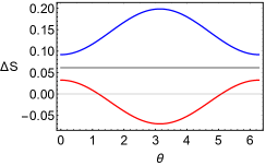
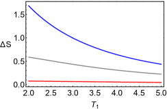
Figure 1: Upper (blue) and lower (red) bounds for the difference of entropies $\Delta S$ (a) as a function of the angle between the Bloch vectors $\theta$ between two thermal equilibrium states with temperature $T_{1}=10$ and (b) as a function of temperature $T_{1}$ with fixed $\theta=\pi/4$. In both cases, we assume $T_{2}=15$, $|h|=\sqrt{61}$, and $|\mathfrak{h}|=\sqrt{17}$. The gray curves correspond to the analytic result.

In fig. 1, the upper and lower bounds of $\Delta S$ are shown for a qubit system as a function of the angle $\theta$ between the Bloch vectors $\mathbf{h}$ and $\boldsymbol{\mathfrak{h}}$. One can see that these limits have a minimum value when the Bloch vectors are parallel and a maximum when they are antiparallel as previously discussed. In fig. 1, the plot of $\Delta S$ is shown as a function of temperature $T_{1}$ with fixed $T_{2}$. Here, one can see that the difference between the bounds and the analytic curve in gray goes down as the temperature increases. This is due to the fact that, as the temperature increases the density matrices $\hat{\rho}_{1}$ and $\hat{\rho}_{2}$ become more and more similar to the most mixed state $\mathbf{I}/2$ (e.g., a spin system where the probability of being up and down is the same), independently of the Hamiltonians $\hat{H}_{1}$ and $\hat{H}_{2}$.

V Harmonic oscillator with a time-dependent frequency

The time dependent harmonic oscillator husimi has been a paradigmatic model in quantum mechanics dodonov . This kind of oscillator may have exact solutions and can be used to obtain statistical properties of the electromagnetic field as antibunching and squeezing mandal . Additionally, a scheme to calculate the Franck–Condon factors for two one-dimensional harmonic oscillators have been studied in octavio .

In this section, the study of the bounds for the harmonic oscillator with a time dependent frequency is presented making use of the time dependent invariant operators of the Hamiltonian, although other different methods can be used e.g. using the Heisenberg operators at two different times. The Hamiltonians are given at two different times, i.e., $\hat{H}_{1}=\hat{H}(t)$ and $\hat{H}_{2}=H(t^{\prime})$. The Hamiltonian of the system is

$$\hat{H}(t)=\frac{1}{2}(\hat{p}^{2}+\omega^{2}(t)\hat{q}^{2})\,,$$ (15)

which has a the time dependent invariant operator $\hat{A}(t)=i(\epsilon(t)\hat{p}-\dot{\epsilon}(t)\hat{q})/\sqrt{2}$, with $\epsilon(t)$ being a solution of the classical equation $\ddot{\epsilon}(t)+\omega^{2}(t)\epsilon(t)=0$ with the initial conditions $\epsilon(0)=1$, $\dot{\epsilon}(0)=i$. This operator satisfies the bosonic commutation relation $[\hat{A}(t),\hat{A}^{\dagger}(t)]=1$ implying the property $\dot{\epsilon}(t)\epsilon^{*}(t)-\epsilon(t)\dot{\epsilon}^{*}(t)=2i$.

From this it is possible to define the integral of motion operator $\hat{A}^{\dagger}(t)\hat{A}(t)$, which has the eigenfunctions

$$\phi_{n}(x,t)=\left(\frac{\epsilon^{*}(t)}{2\,\epsilon(t)}\right)^{n/2}\frac{e^{i\frac{\dot{\epsilon}(t)}{2\,\epsilon(t)}x^{2}}}{\sqrt{n!\,\epsilon(t)\pi^{1/2}}}\,H_{n}\left(\frac{x}{|\epsilon(t)|}\right)\,.$$ (16)

These eigenfunctions form a complete orthonormal set at any time, i.e., $\int dx\,\phi_{m}^{*}(x,t)\phi_{n}(x,t)=\delta_{nm}$, and satisfy also the closure condition $\sum_{n}\phi_{n}^{*}(x,t)\phi_{n}(x^{\prime},t)=\delta(x-x^{\prime})$. In order to obtain the upper and lower bounds of $\Delta S$, one needs to calculate the mean values of the Hamiltonian at any time and the value $\textrm{Tr}(e^{-\beta\hat{H}(t^{\prime})}\hat{H}(t))$. To perform these calculations, it is convenient to write the Hamiltonian at a time $t^{\prime}$ in terms of the operators at time $t$, i.e.,

$$\hat{H}(t^{\prime})=\alpha(t,t^{\prime})\hat{K}_{-}(t)+\alpha^{*}(t,t^{\prime})\hat{K}_{+}(t)+\gamma(t,t^{\prime})\hat{K}_{0}(t)\,,$$ (17)

where we have defined the functions

$$\alpha(t,t^{\prime})=\frac{1}{2}(\dot{\epsilon}^{*2}(t)+\omega^{2}(t^{\prime})\epsilon^{*2}(t)),\quad\gamma(t,t^{\prime})=|\dot{\epsilon}(t)|^{2}+\omega^{2}(t^{\prime})|\epsilon(t)|^{2}\,,$$

which satisfy the relation $4\omega^{2}(t^{\prime})=\gamma^{2}(t,t^{\prime})-4|\alpha(t,t^{\prime})|^{2}$, and the operators $\hat{K}_{-}(t)=\hat{A}^{2}(t)/2$, $\hat{K}_{+}(t)=\hat{A}^{\dagger 2}(t)/2$, and $\hat{K}_{0}(t)=(\hat{A}(t)\hat{A}^{\dagger}(t)+\hat{A}^{\dagger}(t)\hat{A}(t))/4$ are the generators of the SU(1,1) group. Thus, the mean value of $\hat{H}$ at time $t$ in the $t^{\prime}$ state is

$$\frac{1}{Z(\hat{H}(t^{\prime}),T)}{\rm Tr}(e^{-\beta\hat{H}(t^{\prime})}\hat{H}(t))=\frac{1}{Z(\hat{H}(t^{\prime}),T)}\sum_{n=0}^{\infty}\langle n,t|e^{-\beta\hat{H}(t^{\prime})}\hat{H}(t)|n,t\rangle\,,$$

which gives the result (see appendix A)

$$\frac{1}{Z(\hat{H}(t^{\prime}),T)}{\rm Tr}(e^{-\beta\hat{H}(t^{\prime})}\hat{H}(t))=\frac{\omega^{2}(t)+\omega^{2}(t^{\prime})}{4\omega(t^{\prime})}\coth\left(\frac{\omega(t^{\prime})}{2T}\right)\,.$$ (18)

This expression only depends on the frequencies at the different times and the temperature and not in the classical solutions $\epsilon(t)$ and $\epsilon(t^{\prime})$ which greatly simplify their calculation. One can notice that the mean value at time $t$ of the Hamiltonian ${\rm Tr}(e^{-\beta\hat{H}(t)}\hat{H}(t))/Z(\hat{H}(t),T)$ can be obtained from the previous expression making $t^{\prime}=t$ that provides the result

$$\frac{1}{Z(\hat{H}(t),T)}{\rm Tr}(e^{-\beta\hat{H}(t)}\hat{H}(t))=\frac{\omega(t)}{2}\coth\left(\frac{\omega(t)}{2T}\right)\,,$$ (19)

Finally from Eq. (18) the following bounds for the difference of the entropy are obtained

$$\frac{1}{2T_{2}}\left(\omega(t^{\prime})\coth\left(\frac{\omega(t^{\prime})}{2T_{2}}\right)-\frac{\omega^{2}(t^{\prime})+\omega^{2}(t)}{2\omega(t)}\coth\left(\frac{\omega(t)}{2T_{1}}\right)\right)\leq\Delta S\leq$$

$$\leq\frac{1}{2T_{1}}\left(\frac{\omega^{2}(t^{\prime})+\omega^{2}(t)}{2\omega(t^{\prime})}\coth\left(\frac{\omega(t^{\prime})}{2T_{2}}\right)-\omega(t)\coth\left(\frac{\omega(t)}{2T_{1}}\right)\right)$$ (20)

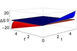
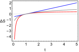
Figure 2: (a) Upper (blue), lower (red) bounds and analytical expression (gray) for the difference of entropies $S_{2}(T_{2},t^{\prime})-S_{1}(T_{1},t)$ for a harmonic oscillator with time dependent frequency $\omega(t)=\sqrt{t}$, with equal temperatures $T_{1}=T_{2}=10$. (b) a 2D cut of the previous plot for $t^{\prime}=1$.

To exemplify the use of the previous results, we analyze two different cases for $\omega(t)$. The case $\omega(t)=\omega_{0}\sqrt{1+\eta\,t}$ has been studied in agarwal , where the authors demonstrate the presence of nonclassical effects of light as squeezing and antibunching. The other example corresponds to the case where $\omega(t)=\omega_{0}\sqrt{1+\eta\,\cos(\Omega t)}$, which can describe the electromagnetic field inside a Paul trap and was first studied in paul . Additionally to these examples, we discuss the case where the harmonic oscillator Hamiltonian is constructed using the time dependent invariant operators $\hat{H}=\omega(t)\left(\hat{A}^{\dagger}(t)\hat{A}(t)+1/2\right)$, since the eigenfunctions of this operator are known.

In the case of $\omega(t)=\omega_{0}\sqrt{1+\eta\,t}$, the solutions to the equation $\ddot{\epsilon}(t)+\omega^{2}(t)\epsilon(t)=0$ are the Airy functions and their derivatives. In fig. 2, the time dependence of the bounds for $\Delta S$ are shown for a system where $\omega(t)=\sqrt{t}$ for fixed temperatures $T_{1}=T_{2}=10$. In this plot, the gray function corresponds to the analytic solution of $S_{2}(T_{2},t^{\prime})-S_{1}(T_{1},t)$. In fig. 2, one can see that there is a region ($t<t^{\prime}=1$) where both the analytical and the limits for $\Delta S$ are negative and some other region ($t>t^{\prime}=1$) where these quantities are positive.

When the frequency has an oscillatory dependence on time, as the one observed in the Paul traps with $\omega(t)=\omega_{0}\sqrt{1+\eta\,\cos(\Omega t)}$, the solution to the equation $\ddot{\epsilon}(t)+\omega^{2}(t)\epsilon(t)=0$ is given by the Mathieu functions and their derivatives. In fig. 3, the dependence of $\Delta S$ in terms of time $t^{\prime}$ is shown for two cases $T_{1}=T_{2}$ and $T_{1}>T_{2}$ for fixed time $t=0.1$ and the explicit frequency $\omega(t)=\sqrt{1+\cos(2t)/2}$. In both cases, the minimum values of the difference of the entropy occurs when the frequency (dashed curve) has a maximum and a maximum value corresponds to the case where the frequency has a minimum. Also it is worth noticing that the minimal difference between the limits and the analytic solution occurs when $\Delta S$ is minimal and has a maximum when $\Delta S$ also has a maximum.

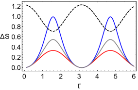
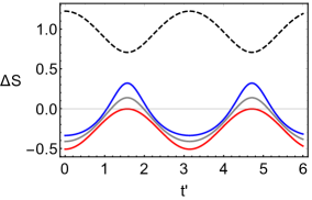
Figure 3: Upper (blue) and lower (red) bounds for the difference of the entropies $\Delta S(t,t^{\prime})$ as a function of $t^{\prime}$ for a time-dependent frequency harmonic oscillator ($\omega(t)=\sqrt{1+\cos(2t)/2}$) between two thermal equilibrium states with temperatures (a) $T_{1}=T_{2}=10$ at the fixed time $t=0.1$ and (b) $T_{1}=15$, $T_{2}=10$ at the fixed time $t=3$. The dashed curve corresponds to the plot of the frequency.

When the Hamiltonian of the system is given by the time dependent invariants

$$\hat{H}(t)=\frac{1}{2}(\hat{P}^{2}(t)+\omega^{2}(t)\hat{Q}^{2}(t))\,,$$ (21)

with the operators $\hat{Q}(t)=(\hat{A}+\hat{A}^{\dagger})/\sqrt{2\omega(t)}$ and $\hat{P}(t)=i\sqrt{\omega(t)/2}(\hat{A}^{\dagger}-\hat{A})$ expressed in terms of the integrals of motion. This Hamiltonian can be interpreted as a degenerated parametric amplifier in the standard bosonic operators with time dependent frequency i.e., $\hat{H}(t)=\nu(t)(\hat{a}^{\dagger}\hat{a}+1/2)-(g^{*}(t)\hat{a}^{\dagger 2}+g(t)\hat{a}^{2})$.

Using the eigenfunctions of the operators $\hat{A}^{\dagger}(t)\hat{A}(t)$ and $\hat{A}^{\dagger}(t^{\prime})\hat{A}(t^{\prime})$, one has

$$\textrm{Tr}(e^{-\beta\hat{H}(t^{\prime})}\hat{H}(t))=\omega(t)\sum_{n,m=0}^{\infty}e^{-\beta\,\omega(t^{\prime})(m+\frac{1}{2})}\left(n+\frac{1}{2}\right)\int dx\,dx^{\prime}\,\phi_{n}(x,t)\phi_{m}^{*}(x,t^{\prime})\phi_{n}^{*}(x^{\prime},t)\phi_{m}(x^{\prime},t^{\prime})\,,$$ (22)

where both sums over $n$ and $m$ can be done separately before the integration using the Mehler formula

$$\sum_{j=0}^{\infty}\frac{(\tilde{\eta}/2)^{j}}{j!}H_{j}(y)H_{j}(y^{\prime})=\frac{1}{(1-\tilde{\eta}^{2})^{1/2}}\exp\left(\frac{2\tilde{\eta}yy^{\prime}-(y^{2}+y^{\prime 2})\tilde{\eta}^{2}}{1-\tilde{\eta}^{2}}\right).$$ (23)

The sum over $m$ gives

$$\sum_{m=0}^{\infty}e^{-\beta\omega(t^{\prime})(m+{1}/{2})}\phi_{m}^{*}(x,t^{\prime})\phi_{m}(x^{\prime},t^{\prime})=\frac{e^{-\beta\omega(t^{\prime})}/{2}}{\pi^{1/2}|b(t^{\prime})|(1-e^{-2\beta\omega(t^{\prime})})^{1/2}}$$

$$\times\exp\left\{\frac{2e^{-\beta\omega(t^{\prime})}qq^{\prime}-(q^{2}+q^{\prime 2})e^{-2\beta\omega(t^{\prime})}}{1-e^{-2\beta\omega(t^{\prime})}}\right\}\exp\left\{-i\frac{\dot{\epsilon}^{*}(t^{\prime})}{2\,\epsilon^{*}(t^{\prime})}x^{2}\right\}\exp\left\{i\frac{\dot{\epsilon}(t^{\prime})}{2\,\epsilon(t^{\prime})}x^{\prime 2}\right\},$$ (24)

with $q=x/|\epsilon(t^{\prime})|$ and $q^{\prime}=x^{\prime}/|\epsilon(t^{\prime})|$. While the sum over $n$ is equal to

$$\omega(t)\sum_{n=0}^{\infty}\left(n+\frac{1}{2}\right)\phi_{n}^{*}(x^{\prime},t)\phi_{n}(x,t)=\omega(t)e^{i\frac{\dot{\epsilon}(t)}{2\epsilon(t)}x^{2}}\left(\frac{1}{2}+x\frac{\partial}{\partial x}-\frac{|\epsilon(t)|^{2}}{2}\frac{\partial^{2}}{\partial x^{2}}\right)e^{-i\frac{\dot{\epsilon}(t)}{2\epsilon(t)}x^{2}}\delta(x-x^{\prime});$$ (25)

to obtain this expression, the derivative of the Hermite polynomials $\frac{dH_{n+1}(x)}{dx}=2(n+1)H_{n}(x)$ together with the recursion relation $H_{n+1}(x)=2xH_{n}(x)-\frac{dH_{n}(x)}{dx}$ were used. Substituting Eqs. (24) and (25) into (22), one arrives at the following expression:

$$\textrm{Tr}(e^{-\beta\hat{H}(t^{\prime})}\hat{H}(t))=\frac{\omega(t)e^{-\beta\omega(t^{\prime})/2}}{4(1-e^{-2\beta\omega(t^{\prime})})^{1/2}\left(\tanh\left({\beta\omega(t^{\prime})}/{2}\right)\right)^{3/2}}f(t,t^{\prime})\,,\\$$

with the definition

$$f(t,t^{\prime})=|\epsilon(t)|^{2}|\dot{\epsilon}(t^{\prime})|^{2}+|\dot{\epsilon}(t)|^{2}|\epsilon(t^{\prime})|^{2}-2\,\textrm{Re}\,(\epsilon(t)\dot{\epsilon}^{*}(t))\,\textrm{Re}\,(\epsilon(t^{\prime})\dot{\epsilon}^{*}(t^{\prime}))\,.$$

Notice that the function $f(t,t^{\prime})$ is symmetrical under the interchange of $t$ and $t^{\prime}$, so the same expression can be used to obtain $\textrm{Tr}(e^{-\beta\hat{H}(t)}\hat{H}(t^{\prime}))$.

The previous expression yields to the result

$$\frac{1}{Z(T,\hat{H}(t^{\prime}))}\textrm{Tr}(e^{-\beta\hat{H}(t^{\prime})}\hat{H}(t))=\frac{\omega(t)}{4}\coth\left(\frac{\omega(t^{\prime})}{2T}\right)f(t,t^{\prime})\,,$$ (26)

while the mean value of the energy is

$$E(T,t)=({\omega(t)}/{2})\,\coth\left({\omega(t)}/{2T}\right)\,.$$ (27)

From these expressions, one can see that the difference of the entropies $S(T_{2},t^{\prime})-S(T_{1},t)$ in the system at times $t$ and $t^{\prime}$ has the following bounds:

$$\frac{\omega(t^{\prime})}{2T_{2}}\left(\coth\left(\frac{\beta_{2}\omega(t^{\prime})}{2}\right)-\frac{1}{2}\coth\left(\frac{\beta_{1}\omega(t)}{2}\right)f(t,t^{\prime})\right)\leq S(T_{2},t^{\prime})-S(T_{1},t)\leq$$

$$\leq\frac{\omega(t)}{2T_{1}}\left(\frac{1}{2}\coth\left(\frac{\beta_{2}\omega(t^{\prime})}{2}\right)f(t,t^{\prime})-\coth\left(\frac{\beta_{1}\omega(t)}{2}\right)\right)\,.$$ (28)

While the exact expression of the entropies can be obtained from the expression

$$S(T,t)=\bar{n}(T,t)\ln\big{[}({1+\bar{n}(T,t)})/{\bar{n}(T,t)}\big{]}+\ln(\bar{n}(T,t)+1),\quad\bar{n}(T,t)=(e^{\omega(t)/T}-1)^{-1}\,.$$ (29)

In fig. 4, the upper and lower bounds are plotted in terms of times $t$ and $t^{\prime}$, and in fig. 4 the dependence of these bounds in terms of $T_{1}$ and $T_{2}$ is shown. One can see a small variation in the time dependence and a very steady behavior in terms of temperatures.

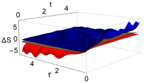
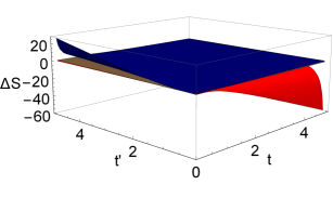
Figure 4: Upper (blue) and lower (red) bounds for the difference of entropies $S(T_{2},t^{\prime})-S(T_{1},t)$ (gray) for a harmonic oscillator with time-dependent frequency $\omega(t)=\sqrt{t}$. Here, (a) $T_{1}=T_{2}=10$ and (b) $t=5$ and $t^{\prime}=10$.

VI Summary and concluding remarks

When a thermal equilibrium system interacts with an external source, either by interchanging particles or only energy, its thermodynamic quantities as the entropy, internal energy and Helmholtz and Gibbs potentials present a change that can be sudden or not depending on the type of interaction with the environment. The main results of our work are the following: we demonstrated that the change in these quantities has upper and lower bounds when the system achieves thermal equilibrium after the interaction. Using the relative entropy between two thermal equilibrium states, the upper and lower bounds of the difference of entropies $\Delta S$ and the Helmholtz and Gibbs potentials were obtained. In the case where the thermal equilibrium states are expressed in terms of the Hamiltonian eigenvectors, these bounds can be written as a sum of the Franck–Condon factors of the two systems. From this, our results can be of interest in the measurement of the vibronic structure of electronic lines in molecules. The possibility of use this bounds to approximate the analytic values is also discussed as the limits can be obtained through the calculation of mean values of the Hamiltonians and the number operator before and after a sudden interaction between the system and an environment.

As examples of applications of the general theory, the bounds for the difference of the entropy are studied for an arbitrary qubit system. In this case, we showed that the bounds have a minimal difference when the Bloch vectors of the Hamiltonians from the initial and final equilibrium states are parallel and have a maximal difference when the Bloch vectors are antiparallel. Also it is noticed that as both states tend to the most mixed density matrix ($\mathbf{I}/2$) as the temperature increases, then this difference decreases independently of the Hamiltonians.

Also the limits for $\Delta S$ were obtained for a harmonic oscillator with time dependent frequency. The bounds were calculated using the eigenvalues and eigenvectors of the constants of motion of the system for two particular cases: $\omega(t)=\omega_{0}\sqrt{t}$, which has been used to show nonclassical properties, and $\omega(t)=\omega_{0}\sqrt{1+\eta\cos(\Omega t)}$, which describes an electromagnetic field in a Paul trap. These limits were also calculated for a harmonic oscillator Hamiltonian written in terms of the operators $\hat{A}(t)$ and $\hat{A}^{\dagger}(t)$. The results obtained for these systems can be applied to the different potentials that can be approximated by a harmonic oscillator.

Appendix A Harmonic oscillator

To calculate the mean value of the Hamiltonian at time $t$ with respect of the density matrix at time $t^{\prime}$, we use the SU(1,1) algebra decomposition of the Hamiltonian given in Eq. (17). The SU(1,1) generators are $\hat{K}_{+}(t)=\hat{A}^{\dagger}(t)/2$, $\hat{K}_{-}(t)=\hat{A}^{2}(t)/2$, and $\hat{K}_{0}(t)=(\hat{A}^{\dagger}(t)\hat{A}(t)+1/2)/2$. This decomposition allows us to write the exponential operator $e^{-\beta\hat{H}(t^{\prime})}$ as the product of the elements of the algebra $e^{-\beta\hat{H}(t^{\prime})}=e^{A_{+}(t^{\prime},t,T)\hat{K}_{+}}e^{\ln(A_{0}(t^{\prime},t,T))\hat{K}_{0}}e^{A_{-}(t^{\prime},t,T)\hat{K}_{-}}$, where $A_{+}(t^{\prime},t,T)$ and $A_{0}(t^{\prime},t,T)$ are

$$A_{0}(t^{\prime},t,T) = \frac{4\omega^{2}(t^{\prime})}{(2\omega(t^{\prime})\cosh(\omega(t^{\prime})/T)+\gamma(t,t^{\prime})\sinh(\omega(t^{\prime})/T))^{2}}\,,$$

$$A_{+}(t^{\prime},t,T) = -\frac{2\alpha^{*}(t,t^{\prime})\sinh(\omega(t^{\prime})/T)}{2\omega(t^{\prime})\cosh(\omega(t^{\prime})/T)+\gamma(t,t^{\prime})\sinh(\omega(t^{\prime})/T)}\,,$$ (30)

and $A_{-}(t^{\prime},t,T)=A_{+}^{*}(t^{\prime},t,T)$. With this, the partition function of the system can be evaluated using the eigenstates of the operator $\hat{A}^{\dagger}(t)\hat{A}(t)$ as follows:

$${\rm Tr}(e^{-\beta\hat{H}(t^{\prime})})=\sum_{l,m,n=0}^{\infty}c_{l,m}\langle n,t|\hat{A}^{\dagger 2m}e^{\ln A_{0}(t^{\prime},t,T)(\hat{A}^{\dagger}(t)\hat{A}(t)+1/2)/2}\hat{A}^{2l}|n,t\rangle\,.$$

where a Taylor expansion of the exponential for $\hat{A}^{2}(t)$ and $\hat{A}^{\dagger 2}(t)$ was performed, and the coefficients $c_{l,m}$ are given by

$$c_{l,m}=\left(\frac{A_{+}(t^{\prime},t,T)}{2}\right)^{m}\left(\frac{A_{+}^{*}(t^{\prime},t,T)}{2}\right)^{l}\frac{1}{m!\,l!}\,.$$

This sum can be rewritten as

$${\rm Tr}(e^{-\beta\hat{H}(t^{\prime})})=A_{0}^{1/4}(t^{\prime},t,T)\sum_{n,m=0}^{\infty}\frac{A_{0}^{n/2}(t^{\prime},t,T)n!}{(m!)^{2}(n-2m)!}\left(\frac{|A_{+}(t^{\prime},t,T)|^{2}}{4A_{0}(t^{\prime},t,T)}\right)^{m}\,,$$

this infinite sum can be truncated for values where the factorial $(n-2m)!<0$ ($m>n/2$). So the previous equation can be expressed in terms of the Legendre polynomials $P_{n}(z)$

$${\rm Tr}(e^{-\beta\hat{H}(t^{\prime})})=A_{0}^{1/4}(t^{\prime},t,T)\sum_{n=0}A_{0}^{n/2}(1-x)^{n/2}P_{n}\left(\frac{1}{\sqrt{1-x}}\right)\,,$$

with $x=\frac{|A_{+}(t^{\prime},t,T)|^{2}}{A_{0}(t^{\prime},t,T)}$. Finally, using the generating function of the Legendre polynomials the following result is obtained:

$$Z(\hat{H}(t^{\prime}),T)=\frac{A_{0}^{1/4}(t^{\prime},t,T)}{(1-2A_{0}^{1/2}(t^{\prime},t,T)+A_{0}(t^{\prime},t,T)-|A_{+}(t^{\prime},t,T)|^{2})^{1/2}}\,,$$ (31)

using the properties of the classical solutions $\dot{\epsilon}(t)\epsilon^{*}(t)-\epsilon(t)\dot{\epsilon}^{*}(t)=2i$, it can be seen that the partition function gives the standard result

$$Z(\hat{H}(t^{\prime}),T)=\frac{1}{2\sinh\left(\frac{\omega(t^{\prime})}{2T}\right)}\,.$$ (32)

The mean values of the operators $\hat{K}_{0}(t)$ and $\hat{K}_{\pm}(t)$ can be calculated by differentiating Eq. (31) with respect to the functions $\ln(A_{0}(t^{\prime},t,T))$, $A_{+}(t^{\prime},t,T)$, and $A^{*}(t^{\prime},t,T)$, respectively. This procedure gives the following expressions

$$\frac{1}{Z(\hat{H}(t^{\prime}),T)}{\rm Tr}(e^{-\beta\hat{H}(t^{\prime})}\hat{K}_{0}(t))=\frac{1-A_{0}(t^{\prime},t,T)+|A_{+}(t^{\prime},t,T)|^{2}}{4(1-2A_{0}^{1/2}(t^{\prime},t,T)+A_{0}(t^{\prime},t,T)-|A_{+}(t^{\prime},t,T)|^{2})}\,,$$ (33)

and

$$\frac{1}{Z(\hat{H}(t^{\prime}),T)}{\rm Tr}(e^{-\beta\hat{H}(t^{\prime})}\hat{K}_{+}(t))=\frac{A_{+}^{*}(t^{\prime},t,T)}{2(1-2A_{0}^{1/2}(t^{\prime},t,T)+A_{0}(t^{\prime},t,T)-|A_{+}(t^{\prime},t,T)|^{2})}\,,$$

$$\frac{1}{Z(\hat{H}(t^{\prime}),T)}{\rm Tr}(e^{-\beta\hat{H}(t^{\prime})}\hat{K}_{-}(t))=\frac{A_{+}(t^{\prime},t,T)}{2(1-2A_{0}^{1/2}(t^{\prime},t,T)+A_{0}(t^{\prime},t,T)-|A_{+}(t^{\prime},t,T)|^{2})}\,,$$ (34)

then substituting Eqs. (33) and (34) into (17) and using the property $\dot{\epsilon}(t)\epsilon^{*}(t)-\epsilon(t)\dot{\epsilon}^{*}(t)=2i$, we obtain the mean value of $\hat{H}(t)$ in the state $e^{-\beta\hat{H}(t^{\prime})}/Z(\hat{H}(t^{\prime}),T)$ given in Eq. (18).

References

- (1) P.A.M. Dirac, The Principles of Quantum Mechanics (Clarendon Press, Oxford, 1981).
- (2) E. Schrödinger, Ann. Phys. 79, 361 (1926).
- (3) E. Schrödinger, Ann. Phys. 81, 109 (1926).
- (4) L. Landau, Z. Phys. 45, 430 (1927).
- (5) J. von Neumann, Götinger Nachrinchten 11, 245 (1927).
- (6) J. von Neumann, Mathematical foundations of quantum mechanics (Princeton University Press, Princeton, 1955).
- (7) C. Tsallis, Nonextensive Statistical Mechanics and Thermodynamics: Historical Background and Present Status (Springer Berlin Heidelberg, Berlin, 2001).
- (8) A. Renyi, Probability Theory (Dover Publications Inc., New York, 2012).
- (9) E. H. Lieb and M. B. Ruskai, J. Math. Phys. 14, 1938 (1973).
- (10) E. A. Carlen, Lett. Math. Phys. 83, 107 (2008).
- (11) M. B. Ruskai, J. Math. Phys. 43, 4358 (2002).
- (12) M. B. Ruskai, J. Math. Phys. 46, 019901 (2005).
- (13) A. Huzihiro, Commun. Math. Phys. 18, 160 (1970).
- (14) J. Goold, M. Huber, A. Riera, L. del Rio, and P. Skrzypczyk, J. of Phys. A 49, 143001 (2016).
- (15) J. M. R. Parrondo, Nat. Phys., 11, 131 (2015).
- (16) K. Maruyama, F. Nori, and V. Vedral, Rev. Mod. Phys. 81, 1 (2009).
- (17) M. Esposito and C. Van den Broeck, Europhys. Lett. 95, 40004 (2011).
- (18) F. G. S. L. Brandão, M. Horodecki, J. Oppenheim, J. M. Renes, and R. W. Spekkens, Phys. Rev. Lett. 111, 250404 (2013).
- (19) P. Skrzypczyk, Nat. Comm. 5, 4185 (2014).
- (20) P. Faist, Nat. Comm. 6, 7669 (2015).
- (21) P. Strasberg, G. Schaller, T. Brandes, and M. Esposito , Phys. Rev. X 7 021003 (2017).
- (22) M. Campisi and J. Goold, Phys. Rev. E 95, 062127 (2017).
- (23) L. Mancino, M. Sbroscia, E. Roccia, I. Gianani, F. Somma, P. Mataloni, M. Paternostro, and M. Barbieri, arXiv:1702.07164v1 (2017).
- (24) M. B. Plenio, Phys. Lett. A, 263, 281 (1999).
- (25) S. Popescu, Nat. Phys. 2, 754 (2006).
- (26) F. G. S. L. Brandão, Nat. Phys. 4, 873 (2008).
- (27) K. Funo, Y. Watanabe, and M. Ueda, Phys. Rev. A 88, 052319 (2013).
- (28) L. H. Ren and H. Fan, Phys. Rev. A 96, 042304 (2017).
- (29) K. Korzekwa, M. Lostaglio, J. Oppenheim, and D. Jennings, New J. Phys. 18, 023045 (2016).
- (30) A. Figueroa, J. López, O. Castaños, R. López-Peña, M. A. Man’ko, and V. I. Man’ko , J. of Phys. A 48, 065301 (2015).
- (31) J. A. López-Saldívar, O. Castaños, M. A. Man’ko, and V. I. Man’ko, Physica A 491, 64 (2018).
- (32) M. A. Man’ko, V. I. Man’ko, and G. Marmo, Il Nuovo Cimento C 38, 167 (2016).
- (33) M. A. Nielsen and I. L. Chuang, Quantum Computation and Quantum Information: 10th Anniversary Edition (Cambridge University Press, New York, 2011).
- (34) U. Fantz and D. Wnderlich, At. Data Nucl. Data Tables 92, 853 (2006).
- (35) E. V. Doktorov, I. A. Malkin, and V. I. Man’ko, J. Mol. Spectrosc. 77, 178 (1979).
- (36) J. Huh and R. Berger, J. Phys. Conf. Ser. 380, 012019 (2012).
- (37) V.V. Dodonov and V.I. Man’ko, Phys. Lett. A 229, 335 (1997).
- (38) V. N. Chernega, O. V. Man’ko and V. I. Man’ko, J. Russ. Laser Res. 38, 141 (2017).
- (39) K. Husimi, Progr. Theor. Phys. , 9, 381 (1953).
- (40) V. V. Dodonov and V. I. Man’ko, Phys. Rev. A 20, 550 (1979).
- (41) S. Mandal, Opt. Commun., 386, 37 (2017).
- (42) O. Castaños, R. López-Peña, and R. Lemus, J. Mol. Spectrosc. 241, 51 (2007).
- (43) G. S. Agarwal and S. A. Kumar, Phys. Rev. Lett. 67, 3665 (1991).
- (44) W. Paul, Rev. Mod. Phys. 62, 531 (1990).