Review: Long-baseline oscillation experiments as a tool to probe High Energy Models

Abstract

We review the current status of neutrino oscillation experiments, mainly focussed on T2(H)K, NO$\nu$A and DUNE. Their capability to probe high energy physics is found in the precision measurement of the CP phase and $\theta_{23}$. In general, neutrino mass models predicts correlations among the mixing angles that can be used to scan and shrink down its parameter space. We updated previous analysis and presents a list of models that contain such structure.

I Introduction

The upcoming sets of long-baseline neutrino experiments will stablish a new standard in the search for new physics. Two distinct directions arrises, the phenomenolocical approach consists on the seek of new unobserved phenomena that are present in a large class of models. They were extensively studied in the literature and are subdivided into 3 main groups: Non-Standard Interactions (NSI) searches Guzzo et al. (1991); Bolanos et al. (2009); Farzan and Tortola (2017); Ghosh and Yasuda (2017); Tang and Zhang (2017); Liao et al. (2017); Farzan (2016); Blennow et al. (2017); Forero and Huang (2017); Ge and Smirnov (2016); Masud and Mehta (2016); Coloma and Schwetz (2016); Huitu et al. (2016), Light Sterile Neutrinos Boyarsky et al. (2012); Heeger et al. (2013); Gastaldo et al. (2016); Giunti and Zavanin (2015); Gariazzo et al. (2016) and Non-unitarity Miranda et al. (2016); Dutta and Ghoshal (2016); Dutta et al. (2017); Escrihuela et al. (2017); Ge et al. (2017); Hernandez-Garcia and Lopez-Pavon (2017); Das et al. (2017); C and Mohanta (2017). The second approach is more theory based and was less explored. It focus on correlations among neutrino mixing angles predicted by high energy models. Its possibility the test of models that contains no low-energy phenomenological effects different from the Standard Model.

Since the discovery of neutrino oscillations, a plethora of models was realized to tried to explain the origin of the neutrino masses. The first proposal was the See-saw mechanism Magg and Wetterich (1980); Mohapatra and Senjanovic (1980); Schechter and Valle (1981); Wetterich (1981); Foot et al. (1989); Abada et al. (2007) which tried to explain the smallness of neutrino masses ($m_{\nu}$) through a heavy mass scale ($M$) $m_{\nu}\propto M^{-1}$. Another possible path uses loop mechanisms, in which neutrino masses can be suppressed at zeroeth Bonnet et al. (2012) or even first order Aristizabal Sierra et al. (2015). Nevertheless, such theories usually do not explain the structure of the oscillation parameters, as they are merely free parameters.

This changes by the addition of discrete symmetry that controls the pattern of the leptonic mass matrix King et al. (2014); Haba et al. (2001); Chen et al. (2016a). They can predict relations among the neutrino mixing angles Cárcamo Hernández and Long (2017); Dev (2017); Centelles Chuliá et al. (2017); Cárcamo Hernández and Long (2017); Chen et al. (2016b); Dicus et al. (2011); Sruthilaya et al. (2015); Dev et al. (2015); Li and He (2015); Dinh et al. (2016); Ky et al. (2016); Cárcamo Hernández et al. (2017); Frampton et al. (2008) which can be used to constrain the parameter space of such theories Pasquini et al. (2017).

This manuscript is divided in seven section: In section II We describe current and future neutrino oscillation experiments: T2K, NO$\nu$A and DUNE and their simulation. In Section III we briefly discuss the statistical analysis and methods used to scan the parameter space. In Section IV we present the sensitivity to neutrino mixing parameters expected in each experiment. In Section V We review the possibilities to use the $\theta_{23}-\delta_{CP}$ correlation in long-baseline experiments by updating previous analysis of two models Chatterjee et al. (2017a, b). In Section VI We review the possibility of using the $\theta_{13}-\theta_{23}$ correlation by combining long-baseline experiments with reaction measurements of $\theta_{13}$. In Section VII we present a summary of the results.

II Long-baseline Experiments and their Simulation

Here we choose to focus on four experimental setup, two of them are already running: T2K Duffy (2017), NO$\nu$A Childress and Strait (2013) and two had their construction approved: DUNE Acciarri et al. (2015) and T2HK Abe et al. (2015a). Their sensitivity on the two most unknown parameters of the leptonic sector, the CP violation phase and the atmospheric mixing angle, makes them ideal to probe correlations among the mixing angles. As it was shown in Pasquini et al. (2017), they can be used to shrink down the parameter space of predictive models. A short description of each experiment can be found below and on Table 1.

Experiment	Baseline	Size	Target	Expected POT	Peak Energy (GeV)	Status
T2K Duffy (2017)	295 km	22.5 kt	Water	$7.8\times 10^{21}$ $\left(20\times 10^{21}\right)$	0.6	Running (10% total POT)
NO$\nu$A Childress and Strait (2013)	810 km	14 kt	Liq. Scintillator	$3.6\times 10^{21}$	2.0	Running (17% total POT)
DUNE Acciarri et al. (2015)	1300 km	40 kt	Liq. Argon	$1.47\times 10^{21}$	2.5	Start data taking: 2026
T2HK Abe et al. (2015a)	295 km	$2\times 190$ kt	Water	$1.56\times 10^{22}$	0.6	Start data taking: 2026 (2032)

Table 1: Summary of neutrino experiments.

1. T2K : The Tokai to Kamiokande (T2K) experiment Abe et al. (2015b); Duffy (2017) uses the Super-Kamiokand Abe et al. (2016) as a far detector for the J-park neutrino beam. Which consists of an off-axis (by a $2.5^{\circ}$ angle) predominantly muon neutrino flux with energy around 0.6 GeV. The Super-Kamiokande detector is a 22.5 kt water tank located at 295 from the J-park facility. It detects neutrino through the Cherenkov radiation emitted by a charged particle created via neutrino interaction. There is also a near detector (ND280), thus the shape of the neutrino flux is well known, and the total normalization error reaches $5\%$ for the signal and $10\%$ for the background. T2K is already running and its current results can be found in Haegel (2017) and reaches $7\times 10^{20}$ POT of flux for each neutrino/anti-neutrino mode, which corresponds to 10% of the $7.8\times 10^{21}$ expected approved exposure. There are also plans for extending the exposure to $20\times 10^{21}$ POT.

2. NO$\nu$A : The NuMI Off-axis $\nu_{e}$ Appearance (NO$\nu$A) Patterson (2012); Childress and Strait (2013); Agarwalla et al. (2012) is an off-axis (by a $0.8^{\circ}$ angle) that uses a neutrino beam from the Main Injector of Fermilab’s beamline (NuMI). This beam consists of mostly muon neutrinos with energy around 2 GeV traveling through 810 km until arriving at the 14 kt Liquid Scintillator far detector placed at Ash River, Minnesota. The far and near detectors are highly active tracking calorimeter segmented by hundreds of PVP cells and can give a good estimate of the total signal and background within an error of $5\%$ and $10\%$ of total normalization error respectively. The planned exposure consists of a $3.6\times 10^{21}$ POT that can be achieved in 6 years of running time, working in $50\%$ in the neutrino mode and $50\%$ in the anti-neutrino mode. NO$\nu$A is already running, current results can be found in Adamson et al. (2017a, b).

3. DUNE :: The Deep Underground Neutrino Experiment (DUNE) Acciarri et al. (2016a, 2015); Strait et al. (2016); Acciarri et al. (2016b); Kemp (2017) is a long baseline next generation on-axis experiment also situated in Fermilab. It flux will be generated at the LBNF neutrino beam to target a 40kt Liquid Argon time chamber projection (LarTPC) located 1300 km away from the neutrino source at Sanford Underground Research Facility (SURF). The beam consists of mostly muon neutrinos of energy around 2.5 GeV and expects a total exposure of $1.47\times 10^{21}$ POT running 3.5 years in neutrino mode and 3.5 years in anti-neutrino mode. The Near and Far detectors are projected to obtain a total signal (background) normalization uncertainty of 4% (10%). The experiment is expected to start taking data around 2026.

4. T2HK: The Tokai to Hyper-Kamiokande (T2HK) Abe et al. (2011); Hyp (2016); Abe et al. (2015a); Yokoyama (2017); Migenda (2017) is an upgrade of the successful T2K experiment at J-Park. It uses the same beam as its predecessor T2K, an off-axis beam from the J-Park facility 295 km away from its new far detector: a two water Cherenkov tank with 190 kt of fiducial mass each. The expected total power is $1.56\times 10^{22}$ POT to be delivered within 2.5 yrs of neutrino mode and 7.5 yrs of anti-neutrino mode in order to obtain a similar number of both neutrino types. The new design includes improvements in the detector systems and particle identification that are still in development. For simplicity, we take similar capability as the T2K experiment and will assume a 5% (10%) of signal (background) normalization error. The first data taking is expected to start with one tank in 2026 and the second tank in 2032.

In order to perform simulation of any neutrino experiment, the experimental collaboration uses Monte Carlo Methods, which can be performed through several event generators such as GENIE Andreopoulos et al. (2010), FLUKA Battistoni et al. (2009) and many others. see PDG Patrignani et al. (2016) for a review. Such techinique requires an enormous computational power and detector knowledge, as it relies on the simulation of each individual neutrino interaction and how its products evolve inside of the detector. A simpler, but faster, simulation can be accomplished by using a semi-analitic calculation of the event rate integral Huber et al. (2005),

$$N_{i}(\nu_{\beta}\rightarrow\nu_{\alpha})=\int_{E_{i}-\Delta E_{i}/2}^{E_{i}+\Delta E_{i}/2}{K_{\nu_{\alpha}}(E,E^{\prime})\phi_{\nu_{\beta}}(E)P_{\beta\alpha}(E)\sigma(E)dEdE^{\prime}}.$$ (1)

$N_{i}$ is the number of detected neutrinos with energy between $E_{i}-\Delta E_{i}/2$ and $E_{i}+\Delta E_{i}/2$. $\phi_{\nu_{\beta}}(E)$ describes the flux of neutrino $\nu_{\beta}$ arriving at the detector. $P_{\beta\alpha}$ is the oscillation probability and $\sigma(E)$ the detection cross section of the detection reaction.

$K_{\nu_{\alpha}}(E,E^{\prime})$, also known as migration matrix, describes how the detector interpretes a $\alpha$ neutrino with energy $E$ being detected at energy $E^{\prime}$ and summarizes the effect of the Monte Carlo simulation of the detector into a single function. A perfect neutrino detector is described by a delta function: $K_{\nu_{\alpha}}(E,E^{\prime})=\delta(E-E^{\prime})$ while a more realistic simulation can use a Gaussian,

$$K_{\nu_{\alpha}}(E,E^{\prime})=\frac{e^{-\frac{(E-E^{\prime})^{2}}{2\delta E^{2}}}}{\sqrt{2\pi}\delta E},$$ (2)

where $\delta E$ parametrizes the error in the neutrino energy detection. Or a migration matrix provided by the experimental collaboration.

The public available software GLoBES Huber et al. (2005, 2007) follows this approach and is commonly used to perform numerical simulation of neutrino experiments. There is also another tool, the NuPro packedge Ge that will be publicly released soon. All the simulations in this manuscript are performed using GLoBES.

III Statistical Analysis and probing models: A brief Discussion

We are interested in a rule to distinguish between two neutrino oscillation models that can modify the spectrum of detected neutrinos in a long-baseline neutrino experiment. From the experimental point of view, one may apply a statistical analysis to quantitatively decide between two (or more) distinct hypothesis given a set of data points $H_{\rm real}$.

Each model (${\rm M}_{i}$) will define a probability distribution function (p.d.f), $f\left(t|{\rm M}_{i}\right)$. Where the statistic test function $t$ depends on the real data points and the model parameters $\theta_{i}$, $i=1,2..$. The best fit of a model are defined as the values of the model parameters that maximize the p.d.f function: $f_{0}(M_{i})={\rm Max}[f\left(H_{\rm real},\theta^{1}_{i}|{\rm M}_{i}\right)]$. Thus, one can reject model $M_{2}$, over model $M_{1}$ by some certain confidence level $n$ if,

$$\frac{f_{0}(M_{2})}{f_{0}(M_{1})}\leq C_{n}.$$ (3)

$C_{n}$ is a constant that depend on the probability test, the number of parameters and the confidence level $n$.

From the theoretical point of view, the real data points were not yet measured, this means that in order to find the expected experimental sensitivity we need to produce pseudo-data points $H_{\rm real}$ by adding an extra assumption on which model is generating the yet-to-be-measured data points. That means there are various ways of obtaining sensitivity curves, each of them are described in Table 2.

Cases	pseudo-data	Null Hypothesis	Test Hypotesis
General	Mi	M1	M2
I	Standard-3$\nu$	Standard-3$\nu$	New Model
II	New Model	Standard-3$\nu$	New Model
III	Standard-3$\nu$	New Model	Standard-3$\nu$
IV	New Model	New Model	Standard-3$\nu$

Table 2: Description of the possible hypotesis taken to generate the numerical anallysis. Here, Standard-3$\nu$ means the standard 3 neutrino oscillation.

Although one can always generate the pseudo-data points using any desired model at any point in its parameter space, the usual approach is to assume that the data points are generated by the standard 3 neutrino oscillation (Standard-3$\nu$) model with parameters given by current best fit values. We will use this approach in the work. Current best fit values are described in Table 3 and were taken from  de Salas et al. (2017).

parameter	value	error
$\Delta m_{21}^{2}/10^{-5}$	7.56 $\rm eV^{2}$	(19)
$\Delta m_{31}^{2}/10^{-3}$	2.55 $\rm eV^{2}$	(4)
$\sin^{2}\theta_{12}$	0.321	(18)
$\sin^{2}\theta_{13}$	0.02155	(90)
$\sin^{2}\theta_{23}$	0.430	(20)
$\delta_{\rm CP}/\pi$	1.40	(31)

Table 3: Current best fit values of Standard-3$\nu$ as given by  de Salas et al. (2017). Notice that Normal Hierarchy is assumed.

III.1 Frequentist Analysis

The chi-square test James (2006); Cochran (1942); Patrignani et al. (2016) is the most commom statistical analysis choosen to teste the compatibility between the experimental data and the expected outcome of a given neutrino experiment. It bases on the construction of a Gaussian chi-squared estimator ($\chi^{2}$) so that $f(t|Model)=Ne^{-\chi^{2}/2}$. This means that the best fit values are obtained by the set of values that globaly minimizes the function $\chi^{2}$. For long-baseline neutrino oscillation experiments the chi-square function can be devided into three factors,

$$\chi^{2}=\chi^{2}_{\rm data}+\chi^{2}_{\rm sys}+\chi^{2}_{\rm prior}.$$ (4)

Where $\chi^{2}_{\rm data}$ in the simplest case reduces to a Poissonian Pearson’s statistic

$$\chi^{2}_{\rm data}=\sum_{i}^{N}\left[\frac{N_{i}^{\rm obs}-(1-a)N_{i}^{s}-(1-b)N_{i}^{b}}{\sqrt{N_{i}^{\rm obs}}}\right]^{2}.$$ (5)

$N_{i}^{\rm obs}$ is the number of observed neutrino in the bin $i=1,2,3..N$ and are the pseudo-data points generated by a given model. $N_{i}^{s}$ ($N_{i}^{b}$) is the signal (background) observed neutrinos as expected by a given model and depend on the model parameters. The $\chi^{2}_{\rm sys}$ comprises the experimental uncertanties and systematics. For the $\chi^{2}$ in Eq. 5, it is given by,

$$\chi^{2}_{\rm sys}=\left(\frac{a}{\sigma_{a}}\right)^{2}+\left(\frac{b}{\sigma_{b}}\right)^{2}.$$ (6)

Here, $\sigma_{a}$ ($\sigma_{b}$) is the total normalization error in the signal (background) flux. Finally, $\chi^{2}_{\rm prior}$ contains all the prior information one wishes to include in the model parameters. In this work we will assume $\chi^{2}_{\rm prior}=0$ unless stated otherwise.

The exponential nature of the chi-squared estimator makes it straigntfoward to find the confidence levels for the model parameters. It sufices to define the function,

$$\Delta\chi^{2}=\chi^{2}_{\rm min}(\theta_{i}|M_{2})-\chi^{2}_{{\rm min}}(M_{1}),$$ (7)

where $\chi^{2}_{{\rm min}}(M_{1})$ is the chi-squared function assuming model $M_{1}$ calculated in its best fit and $\chi^{2}_{\rm min}(\theta_{i}|M_{2})$ is the chi-squared function assuming model $M_{2}$ minimized over all the desired free parameters. Thus, the confidence levels are obtained by finding the solutions of

$$\Delta\chi^{2}\leq A_{n}.$$ (8)

$\theta_{i}$ are all the fixed parameters of model $M_{2}$ and $A_{n}$ are the constants that define the probability cuts and depend on the number of parameters in $\chi^{2}(\theta_{i}|M_{2})$ and the confidence probability. For $n\sigma$ intervals and one parameter, $A_{n}=n^{2}$.

Notice that $\Delta\chi^{2}$ is in fact a function of the parameters one assumes to generate the pseudo-data points, which we call True Values and denote $\theta_{i}(\rm True)$ and the parameters of the model we wish to test, which we call Test Values and denote $\theta_{i}(\rm Test)$.

IV Measurement of Oscillation parameters in Long-baseline Experiments

The main goal of long-baseline experiments is to measure with high precision the two most unknown oscillation parameters: the CP phase and the atmospheric mixing angle $\theta_{23}$ through the measurement of the neutrino/anti-neutrino $\nu_{\mu}\rightarrow\nu_{\mu}$ survival and $\nu_{\mu}\rightarrow\nu_{e}$ transition of neutrinos from the beamline. In special, only the transition is sensitive to $\delta_{\rm CP}$ and described, to first order in matter effects, by the probability function below.

$$P\left(\nu_{\mu}\rightarrow\nu_{e}\right)= 4c_{13}^{2}s^{2}_{13}s_{23}^{2}\sin^{2}\Delta_{31}$$ (9)

$$+8c_{13}^{2}s_{12}s_{13}s_{23}(c_{12}c_{23}\cos\delta_{\rm CP}-s_{12}s_{13}s_{23})\cos\Delta_{32}\cos\Delta_{31}\cos\Delta_{21}$$ (10)

$$-8c_{13}^{2}c_{12}c_{23}s_{12}s_{13}s_{23}\sin\delta_{\rm CP}\sin\Delta_{32}\sin\Delta_{31}\sin\Delta_{21}$$ (11)

$$+4s_{12}^{2}c_{13}^{2}(c_{12}^{2}c_{23}^{2}+s^{2}_{12}s_{23}^{2}s_{13}^{2}-2c_{12}c_{23}s_{12}s_{23}s_{13}\cos\delta_{\rm CP})\sin^{2}\Delta_{21}$$ (12)

$$-8c_{13}^{2}s_{13}^{2}s_{23}^{2}\frac{aL}{4E}(1-2\sin_{13}^{2})\cos\Delta_{32}\sin\Delta_{31}$$ (13)

$$+8c_{13}^{2}s_{13}^{2}s_{23}^{2}\frac{a}{\Delta m^{2}_{31}}(1-2\sin_{13}^{2})\sin^{2}\Delta_{31}.$$ (14)

Where $c_{ij}=\cos\theta_{ij}$, $s_{ij}=\sin\theta_{ij}$, $\Delta_{ij}=\Delta m_{ij}^{2}L/4E$ and $a=2\sqrt{2}G_{\rm F}n_{e}E$. $G_{\rm F}$ is the fermi constant and $n_{e}$ is the electron density in the medium. $E$ is the neutrino energy and $L$ the baseline of the experiment and are choosen to obey $L/E\sim 500$ in order to enhance the effect of the CP phase. The anti-neutrino probability is obtained by change $a\rightarrow-a$ and $\delta_{\rm CP}\rightarrow-\delta_{\rm CP}$. Thus, the difference betweem neutrino and anti-neutrino comes from matter effects and the CP phase.

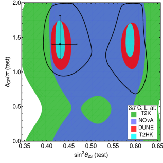
Figure 1: Expected sensitivity regions of $\sin^{2}\theta_{23}(test)$ versus $\delta_{CP}(test)$ assuming as the true and test model the standard-3$\nu$ paradigm for the three long-baseline detectors discussed: (1) T2K (Green), (2) NO$\nu$A (Blue), (3) DUNE (Red) and (4) T2HK (Cyan). The black curve is current 90% C. L. and the black point is the current best fit given in Table 3. Notice that within this assumptions the octant would remain unresolved even at 3$\sigma$ C.L.

It turns out that the T2HK is the most sensitivity to $\delta_{CP}$ as it has a bigger statistic and lower matter effect, and can reach a $8\sigma$ difference between CP conservation and maximal CP-non-conservation Hyp (2016), in contrast with DUNE’s $5.5\sigma$ Acciarri et al. (2016a). In Fig. 1 we plotted the expected allowed regions of $\theta_{23}({test})$ versus $\delta_{\rm CP}({test})$ at $3\sigma$ for each experiment. We assumed the true value of the parameters as those given in Table 3. The black region is the current 90% C. L. region and the black points are the best-fit point. T2HK is the most sensitive experiment in reconstructing both parameters, followed by DUNE. NO$\nu$A and T2K are the first experiments to measure a difference between matter and anti-matter in the leptonic sector, but cannot measure the CP phase with more than 3$\sigma$.

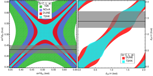
Figure 2: The left (right) panel corresponds to the expected reconstruction of the oscillation parameter $\theta_{23}$ ($\delta_{CP}$). The black line indicates the best fit value given in Table 3 and the gray area corresponds to its $1\sigma$ region. The colored areas represents the regions that the experiments cannot distinguish within more than 3$\sigma$ for: (1) T2K (Green), (2) NO$\nu$A (Blue), (3) DUNE (Red) and (4) T2HK (Cyan). In the right panel we did not included T2K or NO$\nu$A as they cannot reconstruct the CP phase with more than 3$\sigma$.

Notice that the experiments cannot discover the correct octant of $\theta_{23}$ at $3\sigma$, that is, they cannot tell if $\theta_{23}>\pi/4$ (High Octant) or $\theta_{23}<\pi/4$ (Lower Octant) unless they are supplemented by an external prior. This effect is independent of the value of $\theta_{23}$ as can be observed in Fig. 2-Left panel where we plotted the reconstruction of the $\theta_{23}(test)$ given a fixed true value of $\theta_{23}(true)$ of each experiment. The black line corresponds to current best-fit and the gray area is the 1$\sigma$ region. The x-like pattern of the region shows that given any true value of $\theta_{23}$ there is $3\sigma$ region in the correct octant and in the wrong octant. Nevertheless, the octant can be obtained if one incorporates a prior to the $\theta_{13}$ angle Nath et al. (2016); Bora et al. (2015); Minakata et al. (2003) and future prospects on the measurement of $\theta_{13}$ by reactor experiments will allow both DUNE and T2HK to measure the octant if the atmospheric angle does not all inside the region $0.47<\sin^{2}\theta_{23}<0.53$ Sachi Chatterjee et al. (2017).

For completeness, we show in the left panel of Fig. 2 the reconstruction of the $\delta_{\rm CP}(test)$ given a fixed true value of $\delta_{CP}(true)$. The black line represents current best fit and the gray area the $1\sigma$ region. We don’t show the plots for NO$\nu$A or T2K as they cannot reconstruct the CP phase at $3\sigma$. The sensitivity is a little bit worse around maximum CP violation $\delta_{\rm CP}=\pi/2$ or $3\pi/2$ but in general it does not change much when one varies the $\delta_{\rm CP}(true)$.

V $\theta_{23}$ and $\delta_{CP}$ Correlation and Probing Models

In spite of being relatively low energy (< few GeV), neutrino experiments can be a tool to probe high energy physics. Many neutrino mass models predicts relations such as neutrino mass sum rules Spinrath (2017); Buccella et al. (2017); Gehrlein et al. (2016) that can be probed in neutrinoless double beta decay King et al. (2013) and relations among the neutrino mixing parameters. To name a few examples we cite Cárcamo Hernández and Long (2017); Dev (2017); Centelles Chuliá et al. (2017); Cárcamo Hernández and Long (2017). They can be put to test by a scan of the parameter space much like it was done by the LHC in search for new physics. Thus, inspired by the precision power of future long-baseline neutrino experiments, it was shown in Pasquini et al. (2017) that models that predict a sharp correlation between the atmospheric angle and the CP phase can be used to put stringent bounds on parameters of such models.

In general, a predictive neutrino mass model ${\cal M}$ is constructed by imposing a symmetry on the Lagrangian and can be parametrized by a set of free parameters $\phi_{i}$, $i=1,2,...N$ which can be translated into the usual neutrino mixing parameters from the neutrino mass matrix, that is,

$$\theta_{jk}\equiv \theta_{jk}(\phi_{i}),$$ (15)

$$\delta_{\rm CP}\equiv \delta_{\rm CP}(\phi_{i}).$$ (16)

Because of the symmetry on the Lagrangian, not all possible mass matrices are allowed to be generated and the free parameters $\phi_{i}$ may not span the entire space of the mixing parameters $\theta_{ij}$ and $\delta_{\rm CP}$. Thus, in principle, it is possible to probe or even exclude a model if the real best fit falls into a region that the model ${\cal M}$ cannot predict. As an example, in Fig. 3 we plot the allowed parameter space o two discrete symmetry based models, the Warped Flavour symmetry (WFS) model Chen et al. (2016b) - Left and the Revamped $A_{4}$ Babu-Ma-Valle (BMV) model Morisi et al. (2013) - Right. The black curves represents currently unconstrained (Standard-$3\nu$) 90% C. L. regions for the neutrino parameters and the black point the best-fit value, while the blue region represents the $3\sigma$ allowed parameter space of the two models.

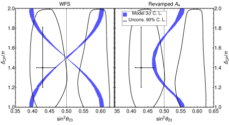
Figure 3: In Blue: Possible parameter values allowed by the two benchmark models: Warped Flavour Symmetry (Left) and Revamped $A_{4}$-BMV (Right). The regions are constructed by varying all the free paramters of the model and selecting those that are allowed at $3\sigma$ in current global fit analysis de Salas et al. (2017). The black line corresponds to curren 90% C. L. region and the black-dot is the best-fit of Table 3. Normal Hierarchy is assumed.

Notice that even for the 3$\sigma$ range the model can only accommodate a much smaller region than the unconstrained. This is a reflex of the symmetries forced upon those models by construction, in WFS a maximal CP phase implies a $\theta_{23}=\pi/4$ and the smaller the CP violation, the farther away from $\pi/4$ the atmospheric angle is. While in BMV a maximal CP phase implies a lower octant atmospheric mixing and it can’t fit a $|\theta_{23}-\pi/4|>0.02\pi$.

By using this approach, a full scan of the parameter space was performed for those two models, in Chatterjee et al. (2017a) for the WFS model and in Chatterjee et al. (2017b) for the Revamped $A_{4}$ model.

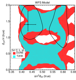
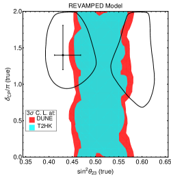
Figure 4: Expected sensitivity regions at which DUNE (Red) or T2HK (Cyan) would not exclude the WFS model (Left) and the revamped BMV model (Right) at $3\sigma$ confidence level. The black contours correspond to 90% C.L. of current global-fit de Salas et al. (2017).

We show in Fig. 4 an updated version of their results. The colored regions represent regions of the parameter space in which the model cannot be excluded with more than $3\sigma$ for DUNE (red) and T2HK (blue) experiment, both T2K and NO$\nu$A cannot probe the CP phase with more than 3$\sigma$, thus, they cannot exclude the model alone.

This means that if future long-baseline experiments measure a specific combination of $\delta_{\rm CP}$ and $\theta_{23}$ as its best fit that does not fall into the colored regions, they may be able to exclude the model. Therefore, those kind of analysis are guidelines to decide which model can or cannot be tested given the future results of DUNE and T2HK and are worth to be performed in any model that contains predictive correlations among the CP phase and the atmospheric mixing, such as Cárcamo Hernández and Long (2017); Dev (2017); Centelles Chuliá et al. (2017); Cárcamo Hernández and Long (2017); Srivastava et al. (2017) and many others. It is also worth mention that combination of long-baseline measurements and reactors can greatly improve the sensitivity of the analysis.

VI $\theta_{13}$ and The atmospheric Octant

The analysis in the last section can be extended to include another type of correlation that tries to explain the smallness of the reactor angle $\theta_{13}\sim O(10^{\circ})$. A general approach common in many models Dicus et al. (2011); Sruthilaya et al. (2015); Dev et al. (2015); Li and He (2015); Dinh et al. (2016); Ky et al. (2016); Cárcamo Hernández et al. (2017); Frampton et al. (2008) imposes a given symmetry on the mass matrix that predicts $\theta_{13}=0$. Which is later spontaneously broken to give a small correction $\delta\theta_{13}\sim O(10^{\circ})$ to the reactor angle. It turns out that in order to generate non-zero $\theta_{13}$ one automatically generates corrections to other mixing angles $\delta\theta_{ij}\neq 0$.

This can be easely observed by considering a toy model that predicts the Tri-bi-maximal mixing matrix,

$$U_{PMNS}=U_{TBM}=\left(\begin{array}[]{ccc}\sqrt{\frac{2}{3}}&\sqrt{\frac{1}{3}}&0\\ \sqrt{\frac{1}{3}}&-\sqrt{\frac{1}{3}}&\sqrt{\frac{1}{2}}\\ -\sqrt{\frac{1}{3}}&\sqrt{\frac{1}{3}}&\sqrt{\frac{1}{2}}\end{array}\right).$$ (17)

Any consistent small correction to the mixing matrix should maintain its unitary character. In special, we can set a correction in the $2-3$ plane via the matrix

$$\delta U_{23}=\left(\begin{array}[]{ccc}1&0&0\\ 0&1&\delta\theta\\ 0&-\delta\theta&1\end{array}\right).$$ (18)

Notice that $\delta U_{23}.\delta U_{23}^{\dagger}=1+O(\delta\theta^{2})$. If we change the mixing matrix by $U_{PMNS}=U_{TBM}\rightarrow U_{TBM}.\delta U_{23}$ then $\theta_{13}=\frac{1}{\sqrt{3}}\left|\frac{\pi}{4}-\theta_{23}\right|$. The general case can be described by a initial mixing matrix $U_{PMNS}=U_{0}$ that is later corrected by a rotation matrix $U_{ij}$,

$$U_{PMNS}=U_{0}\rightarrow U_{PMNS}=U_{ij}.U_{0}\quad{\rm or}\quad U_{0}.U_{ij}$$ (19)

All the possible combinations of corrections from Tri-Bi-MAximal, Bi-Maximal and democratic mixing were considered in Chao and Zheng (2013). In special, one can investigate a general correlation of $\theta_{13}$ to the non-maximality of the atmospheric angle,

$$\theta_{13}=F\left(\delta\theta_{23}\right).$$ (20)

Where $F$ is a function of the correction $\delta\theta_{23}=\left|\frac{\pi}{4}-\theta_{23}\right|$. Long-baseline experiments alone are not too sensitive to changes in the reactor angle, nevertheless, it was shown in Pasquini (2017) that it is possible to use such correlation to probe the parameter space of such models by combining long-baseline and reactor experiments.

This can be accomplished in a model-independend approach by series expanding Eq. 20,

$$\theta_{13}=f(0)+f^{\prime}(0)\left|\frac{\pi}{4}-\theta_{23}\right|\equiv\theta^{0}_{13}+f\left|\frac{\pi}{4}-\theta_{23}\right|.$$ (21)

This encompass both the uncorrelated (standard-3$\nu$) case if one sets $f=0$ and assumes $\theta^{0}_{13}$ as a free parameter and the small correction case by setting $\theta^{0}_{13}=0$ and $f\neq 0$. On table 4 we present many models that contain this kind of correlation and their possible parameters values for $f$ and $\theta^{0}_{13}$.

Model	$f$	$\theta^{0}_{13}[{\rm rad}]$
Frampton et al. (2008)	$\sqrt{2}$	0
Ky et al. (2016); Dinh et al. (2016)	$0.35$	[0,0.35]
Li and He (2015)	$0.1$ or $10$	0.62
Cárcamo Hernández et al. (2017)	$1/\theta_{0}$	[-1,1]
$U_{13}.U_{TBM}$	$6.3$	$0$
$U_{12}.U_{TBM}$	$6.3$	$0$
$U_{TBM}.U_{23}$	$1/\sqrt{3}$	$0$

Model	$f$	$\theta^{0}_{13}[{\rm rad}]$
$U_{BM}.U_{23}U_{13}$	$1/2$	$0$
$U_{TBM}.U_{23}U_{12}$	$2$	$0.157$
$U_{TBM}.U_{23}U_{13}$	$1/\sqrt{2}$	$0$
$U_{TBM}.U_{13}U_{12}$	$2/\sqrt{2}$	$0$
$U_{BM}.U_{13}U_{12}$	$\sqrt{3/2}$	$0$
$U_{BM}.U_{23}U_{12}$	$\sqrt{3/2}$	$0$
$U_{BM}.U_{23}U_{13}$	$1/2$	$0$

Table 4: Summary of models containing reactor and atmospheric angle correlation. All the possible combinations of corrections from Tri-Bi-MAximal, Bi-Maximal and democratic mixing were considered in Chao and Zheng (2013).

On Fig. 6 we update the potential exclusion regions where models of the form $\theta_{13}^{0}=0$ can be excluded for each value of $\sin^{2}\theta_{23}(true)$ at 3$\sigma$ by DUNE+reactors and T2HK+reactors. The true value of $\theta_{13}$ is set to the central value of Table 3 and its error is assumed to be $3\%$. The colored regions represent the regions that cannot be excluded with more than 3$\sigma$. There we can see that models that contain strong correlations ($f>1.9$) or weak correlations ($f<0.8$) can be excluded from any set of atmospheric angle.

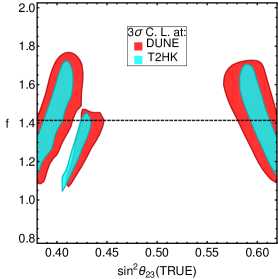
Figure 5: Regions that future neutrino long-baseline oscillation experiments cannot exclude the models that follow Eq. 21 at more than 3$\sigma$ C.L. as a function of the true value of the atmospheric mixing angle for: DUNE(Red) and T2HK(Cyan)

The general case for any $\theta_{13}^{0}$ is presented in Fig. 6 for DUNE on the left panel and for T2HK on right panel for three values of $\sin^{2}\theta_{23}$: 0.43 (Green), 0.5 (Blue) and 0.6 (Red). The region shrinks greatly as the true value of the atmospheric angle goes away from the maximal mixing $\theta_{23}(true)=\pi/4$.

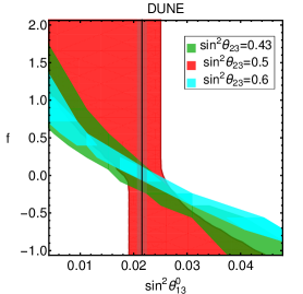
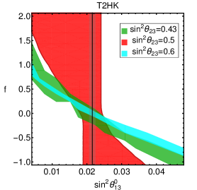
Figure 6: General parameter space regions that cannot be distinguished from the unconstrained relation hypothesis at more than $3\sigma$ by future long-baseline neutrino oscillation experiments in combination with reactor measurements as a function of the two parameters of Eq. 21: $\theta_{13}^{0}$ and $f$. The analysis assumed the central value of the reactor angle as the best-fit given in Table 3 and three values for the atmospheric angle: (1) $\sin^{2}\theta_{23}(true)=0.43$ (Green), (2) $\sin^{2}\theta_{23}(true)=0.5$ (Red) and (3) $\sin^{2}\theta_{23}(true)=0.6$ (Cyan) for DUNE (Left) and T2HK (Right).

VII Summary

The state-of-art of long-baseline neutrino oscillation experiments are T2(H)K, NO$\nu$ and DUNE. They will be capable of reaching very good precision in the reactor and atmospheric mixing angle and will measure for the first time the CP violation phase. This will create an opportunity to put at test a plethora of neutrino mass models that predict values and correlations among the parameters of the PMNS matrix Pasquini et al. (2017); Chatterjee et al. (2017a, b); Srivastava et al. (2017); Ge et al. (2011, 2012).

Here we briefly discuss the fitting approach that quantify the ability of long-baseline experiments to exclude predictive high energy models. Two types of correlations can be used: The $\theta_{23}-\delta_{\rm CP}$ correlation is found in many models containing a variety of symmetries Cárcamo Hernández and Long (2017); Dev (2017); Centelles Chuliá et al. (2017); Cárcamo Hernández and Long (2017); Chen et al. (2016b). Nevertheless, each model in the market may contain a different correlation, and most models are still in need to be analyzed. On the other hand, the $\theta_{13}-\theta_{23}$ correlation can only be probed by combining Long-baseline with reactor experiments, as the former are not sensible enough to $\theta_{13}$ variations. However, we can take a model-independent approach Pasquini (2017) that covers most models that try to explain the smallness of the $\theta_{13}$ angle trough an spontaneous symmetry breaking Dicus et al. (2011); Sruthilaya et al. (2015); Dev et al. (2015); Li and He (2015); Dinh et al. (2016); Ky et al. (2016); Cárcamo Hernández et al. (2017); Frampton et al. (2008). We present a set of figures 4, 5 and 6 containing the potential exclusion regions of each model here analysed that can be used as a benchmark when the future experiments starts to run.

References

- Guzzo et al. (1991) M. M. Guzzo, A. Masiero, and S. T. Petcov, Phys. Lett. B260, 154 (1991).
- Bolanos et al. (2009) A. Bolanos, O. G. Miranda, A. Palazzo, M. A. Tortola, and J. W. F. Valle, Phys. Rev. D79, 113012 (2009), arXiv:0812.4417 [hep-ph] .
- Farzan and Tortola (2017) Y. Farzan and M. Tortola, (2017), arXiv:1710.09360 [hep-ph] .
- Ghosh and Yasuda (2017) M. Ghosh and O. Yasuda, (2017), arXiv:1709.08264 [hep-ph] .
- Tang and Zhang (2017) J. Tang and Y. Zhang, (2017), arXiv:1705.09500 [hep-ph] .
- Liao et al. (2017) J. Liao, D. Marfatia, and K. Whisnant, JHEP 01, 071 (2017), arXiv:1612.01443 [hep-ph] .
- Farzan (2016) Y. Farzan, in 18th International Workshop on Neutrino Factories and Future Neutrino Facilities Search (NuFact16) Quy Nhon, Vietnam, August 21-27, 2016 (2016) arXiv:1612.04971 [hep-ph] .
- Blennow et al. (2017) M. Blennow, P. Coloma, E. Fernandez-Martinez, J. Hernandez-Garcia, and J. Lopez-Pavon, JHEP 04, 153 (2017), arXiv:1609.08637 [hep-ph] .
- Forero and Huang (2017) D. V. Forero and W.-C. Huang, JHEP 03, 018 (2017), arXiv:1608.04719 [hep-ph] .
- Ge and Smirnov (2016) S.-F. Ge and A. Yu. Smirnov, JHEP 10, 138 (2016), arXiv:1607.08513 [hep-ph] .
- Masud and Mehta (2016) M. Masud and P. Mehta, Phys. Rev. D94, 053007 (2016), arXiv:1606.05662 [hep-ph] .
- Coloma and Schwetz (2016) P. Coloma and T. Schwetz, Phys. Rev. D94, 055005 (2016), [Erratum: Phys. Rev.D95,no.7,079903(2017)], arXiv:1604.05772 [hep-ph] .
- Huitu et al. (2016) K. Huitu, T. J. Karkkainen, J. Maalampi, and S. Vihonen, Phys. Rev. D93, 053016 (2016), arXiv:1601.07730 [hep-ph] .
- Boyarsky et al. (2012) A. Boyarsky, D. Iakubovskyi, and O. Ruchayskiy, Phys. Dark Univ. 1, 136 (2012), arXiv:1306.4954 [astro-ph.CO] .
- Heeger et al. (2013) K. M. Heeger, B. R. Littlejohn, H. P. Mumm, and M. N. Tobin, Phys. Rev. D87, 073008 (2013), arXiv:1212.2182 [hep-ex] .
- Gastaldo et al. (2016) L. Gastaldo, C. Giunti, and E. M. Zavanin, JHEP 06, 061 (2016), arXiv:1605.05497 [hep-ph] .
- Giunti and Zavanin (2015) C. Giunti and E. M. Zavanin, Mod. Phys. Lett. A31, 1650003 (2015), arXiv:1508.03172 [hep-ph] .
- Gariazzo et al. (2016) S. Gariazzo, C. Giunti, M. Laveder, Y. F. Li, and E. M. Zavanin, J. Phys. G43, 033001 (2016), arXiv:1507.08204 [hep-ph] .
- Miranda et al. (2016) O. G. Miranda, M. Tortola, and J. W. F. Valle, Phys. Rev. Lett. 117, 061804 (2016), arXiv:1604.05690 [hep-ph] .
- Dutta and Ghoshal (2016) D. Dutta and P. Ghoshal, JHEP 09, 110 (2016), arXiv:1607.02500 [hep-ph] .
- Dutta et al. (2017) D. Dutta, P. Ghoshal, and S. Roy, Nucl. Phys. B920, 385 (2017), arXiv:1609.07094 [hep-ph] .
- Escrihuela et al. (2017) F. J. Escrihuela, D. V. Forero, O. G. Miranda, M. Tórtola, and J. W. F. Valle, New J. Phys. 19, 093005 (2017), arXiv:1612.07377 [hep-ph] .
- Ge et al. (2017) S.-F. Ge, P. Pasquini, M. Tortola, and J. W. F. Valle, Phys. Rev. D95, 033005 (2017), arXiv:1605.01670 [hep-ph] .
- Hernandez-Garcia and Lopez-Pavon (2017) J. Hernandez-Garcia and J. Lopez-Pavon, in Proceedings, Prospects in Neutrino Physics (NuPhys2016): London, UK, December 12-14, 2016 (2017) arXiv:1705.01840 [hep-ph] .
- Das et al. (2017) C. R. Das, J. Maalampi, J. a. Pulido, and S. Vihonen, (2017), arXiv:1708.05182 [hep-ph] .
- C and Mohanta (2017) S. C and R. Mohanta, (2017), arXiv:1708.05372 [hep-ph] .
- Magg and Wetterich (1980) M. Magg and C. Wetterich, Phys. Lett. 94B, 61 (1980).
- Mohapatra and Senjanovic (1980) R. N. Mohapatra and G. Senjanovic, Phys. Rev. Lett. 44, 912 (1980).
- Schechter and Valle (1981) J. Schechter and J. W. F. Valle, Phys. Rev. D23, 1666 (1981).
- Wetterich (1981) C. Wetterich, Nucl. Phys. B187, 343 (1981).
- Foot et al. (1989) R. Foot, H. Lew, X. G. He, and G. C. Joshi, Z. Phys. C44, 441 (1989).
- Abada et al. (2007) A. Abada, C. Biggio, F. Bonnet, M. B. Gavela, and T. Hambye, JHEP 12, 061 (2007), arXiv:0707.4058 [hep-ph] .
- Bonnet et al. (2012) F. Bonnet, M. Hirsch, T. Ota, and W. Winter, JHEP 07, 153 (2012), arXiv:1204.5862 [hep-ph] .
- Aristizabal Sierra et al. (2015) D. Aristizabal Sierra, A. Degee, L. Dorame, and M. Hirsch, JHEP 03, 040 (2015), arXiv:1411.7038 [hep-ph] .
- King et al. (2014) S. F. King, A. Merle, S. Morisi, Y. Shimizu, and M. Tanimoto, New J. Phys. 16, 045018 (2014), arXiv:1402.4271 [hep-ph] .
- Haba et al. (2001) N. Haba, J. Sato, M. Tanimoto, and K. Yoshioka, Phys. Rev. D64, 113016 (2001), arXiv:hep-ph/0101334 [hep-ph] .
- Chen et al. (2016a) P. Chen, G.-J. Ding, F. Gonzalez-Canales, and J. W. F. Valle, Phys. Rev. D94, 033002 (2016a), arXiv:1604.03510 [hep-ph] .
- Cárcamo Hernández and Long (2017) A. E. Cárcamo Hernández and H. N. Long, (2017), arXiv:1705.05246 [hep-ph] .
- Dev (2017) A. Dev, (2017), arXiv:1710.02878 [hep-ph] .
- Centelles Chuliá et al. (2017) S. Centelles Chuliá, R. Srivastava, and J. W. F. Valle, Phys. Lett. B773, 26 (2017), arXiv:1706.00210 [hep-ph] .
- Chen et al. (2016b) P. Chen, G.-J. Ding, A. D. Rojas, C. A. Vaquera-Araujo, and J. W. F. Valle, JHEP 01, 007 (2016b), arXiv:1509.06683 [hep-ph] .
- Dicus et al. (2011) D. A. Dicus, S.-F. Ge, and W. W. Repko, Phys. Rev. D83, 093007 (2011), arXiv:1012.2571 [hep-ph] .
- Sruthilaya et al. (2015) M. Sruthilaya, S. C, K. N. Deepthi, and R. Mohanta, New J. Phys. 17, 083028 (2015), arXiv:1408.4392 [hep-ph] .
- Dev et al. (2015) A. Dev, P. Ramadevi, and S. U. Sankar, JHEP 11, 034 (2015), arXiv:1504.04034 [hep-ph] .
- Li and He (2015) G.-N. Li and X.-G. He, Phys. Lett. B750, 620 (2015), arXiv:1505.01932 [hep-ph] .
- Dinh et al. (2016) D. N. Dinh, N. A. Ky, P. Q. Van, and N. T. H. Vân, (2016), arXiv:1602.07437 [hep-ph] .
- Ky et al. (2016) N. A. Ky, P. Quang Van, and N. T. Hong Van, Phys. Rev. D94, 095009 (2016), arXiv:1610.00304 [hep-ph] .