Numerically solving the relativistic Grad-Shafranov equation in Kerr spacetimes: Numerical techniques

Abstract

The study of the electrodynamics of static, axisymmetric and force-free Kerr magnetospheres relies vastly on solutions of the so called relativistic Grad-Shafranov equation (GSE). Different numerical approaches to the solution of the GSE have been introduced in the literature, but none of them has been fully assessed from the numerical point of view in terms of efficiency and quality of the solutions found. We present a generalization of these algorithms and give detailed background on the algorithmic implementation. We assess the numerical stability of the implemented algorithms and quantify the convergence of the presented methodology for the most established setups (split-monopole, paraboloidal, BH-disk, uniform).

1 Introduction

The so called Grad-Shafranov equation (GSE) (Lüst & Schlüter, 1954; Grad & Rubin, 1958; Shafranov, 1966) appears as the master equation to determine axisymmetric magnetostatic equilibrium configurations. In particular, it has been applied to obtain force-free magnetospheres around Kerr black holes in the context of the energy extraction mechanisms for relativistic jets by Blandford & Znajek (1977). In their seminal work, analytic solutions for the case in which the black hole (BH) spin is small were obtained. More general solutions including arbitrarily large values of the BH specific angular momentum require a numerical evaluation of the solution of the GSE (e.g., MacDonald 1984; Fendt 1997; Uzdensky 2004; Contopoulos et al. 2013; Nathanail & Contopoulos 2014). As an alternative to the solution of the GSE, the topology of the electromagnetic field around a rotating BH has been determined as an asymptotic steady state of force-free degenerate electrodynamics (FFDE) evolution (Komissarov, 2001, 2002, 2004; Tchekhovskoy et al., 2010). Tchekhovskoy et al. (2010) also construct steady state models for BH magnetospheres for a range of spin factors employing General Relativistic Magnetohydrodynamic (GRMHD) simulations in the force-free limit. These time-evolving approaches to reach a steady state usually impose boundary conditions at the outer BH event horizon as well as at the position of an assumed thin accretion disk.

Drawing from previous findings on neutron star magnetospheres, Contopoulos et al. (1999); Contopoulos et al. (2013) presented a numerical scheme for the solution of the GSE in a split-monopole setup. Contopoulos et al. aimed to find a field line configuration passing smoothly through the singular surfaces of the problem (i.e., the light surfaces, as previously suggested by Lee et al. 2000). For that, they implemented a numerical methodology relying vastly on subtle, empirically determined relaxation procedures of all involved functions. In other words, the relaxation to the numerical solution requires recipes which seem to work, but there is no explicit mathematical justification about why they do. The original algorithm of Contopoulos et al. (2013) has later been improved in two ways (Nathanail & Contopoulos, 2014). First, it has been supplemented by further smoothing steps in the numerical algorithm. Second, Nathanail & Contopoulos (2014) also included paraboloidal configurations of the magnetic field. In their study of systems of non-rotating BHs and thin accretion disks, Uzdensky (2004) found a solution to the GSE for a fixed field line angular velocity. He employs the minimization of a suitably chosen error function at the light surfaces in order to mathematically drive the numerical relaxation procedure. A similar approach was followed by Uzdensky (2005) in the case of rotating BHs connected to thin accretion disks.

This paper begins by giving a recapitulation of the GSE and its singular surfaces (sec. 2). With regards to realistic field configurations in BH magnetospheres we formulate the underlying equations of force-free electrodynamics in both the potential and field representation. Subsequently (sec. 3), we present a comprehensive approach to the numerical solution of the GSE. The strategy of minimizing a suitable error function at the light surfaces (LS) (Uzdensky, 2004) is extended to the relaxation procedures of both, the field line angular velocity as well as the current profile. We are able to quantify the numerical errors and, hence, substantiate the quality and stability of the found solutions. In sec. 4, the GSE solution scheme is tested on split-monopole and paraboloidal configurations, as well as the test case of vertical magnetic fields (cf. Contopoulos et al., 2013; Nathanail & Contopoulos, 2014). Furthermore, a current-free solution (as found in Uzdensky, 2005) is reproduced. The BZ process power is studied for the split-monopole configurations in section 5, emphasizing the need for reliable initial data of BH magnetospheres with large spin parameter $a$.

2 Grad-Shafranov equation for relativistic force-free Kerr magnetospheres

The Kerr solution is a suitable approximation of the spacetime in astrophysical scenarios of jet formation. It embodies the geometry of a spinning BH of mass $M$ and specific angular momentum $a=J/M$ (with its dimensionless equivalent $a_{*}=a/M$), where $J$ is the angular momentum. Throughout this work, the speed of light and gravitational constant will be set as $c=G=1$. In Boyer-Lindquist coordinates, the line element of the Kerr metric is

$$\text{d}s^{2} =\>\left(1-\frac{2Mr}{\Sigma}\right)\text{d}t^{2}+\frac{4Mar\sin^{2}\theta}{\Sigma}\>\text{d}t\text{d}\phi$$

$$-\frac{\Sigma}{\Delta}\>\text{d}r^{2}-\Sigma\>\text{d}\theta^{2}-\frac{A\sin^{2}\theta}{\Sigma}\>\text{d}\phi^{2},$$

$$\Sigma:= \>r^{2}+a^{2}\cos^{2}\theta\>,$$

$$A:= \>\left(r^{2}+a^{2}\right)^{2}-\Delta\>a^{2}\sin^{2}\theta\>,$$

$$\Delta:= \>r^{2}-2Mr+a^{2}:=\left(r-r_{+}\right)\left(r-r_{-}\right)\>,$$

where $r_{\pm}$ represent the locations of the outer and inner horizons of the BH, respectively. $r^{*}_{\pm}$ define the locations of the outer and inner ergosurfaces:

$$r_{\pm}=M\pm\sqrt{M^{2}-a^{2}}\quad;\quad r^{*}_{\pm}{(\theta)}=M\pm\sqrt{M^{2}-a^{2}\cos^{2}\theta}.$$ (1)

The frame-dragging frequency induced by the rotation of the BH is

$$\Omega:=\>2aMr/A,$$ (2)

which is also the angular velocity of the (local) zero angular momentum observer or ZAMO (cf. Thorne et al., 1986), i.e., $\Omega=(d\phi/dt)_{\rm ZAMO}$. At the outer event horizon, the frame dragging frequency reads

$$\Omega_{\rm\text{\tiny BH}}:=\Omega(r=r_{+})=\frac{a}{2Mr_{+}}=\frac{a}{r_{+}^{2}+a^{2}}.$$ (3)

The redshift or lapse function is

$$\qquad\qquad\alpha:=\sqrt{\frac{\Sigma\Delta}{A}},$$ (4)

which accounts for the lapse of proper time $\tau$ in the ZAMO frame with respect to the global (Boyer-Lindquist) time $t$, thus, $\alpha=(d\tau/dt)_{\rm ZAMO}$. While the global Boyer-Lindquist observer uses an spatial coordinate basis made by the set of orthogonal vectors $\{\partial_{i}\}=\{\bm{e}_{i}\}$, the local ZAMO observers have an attached tetrad $\{\bm{\hat{e}}_{i}\}=\{\bm{e}_{i}/\sqrt{g_{ii}}\}$, where the Latin index $i$ runs over the three spatial coordinates $(r,\theta,\phi)$. $g_{ii}$ are the diagonal components of the metric tensor, namely

$$g_{rr}=\frac{\Sigma}{\Delta},\qquad g_{\theta\theta}=\Sigma,\qquad g_{\phi\phi}=\frac{A\sin^{2}{\theta}}{\Sigma}.$$

The covariant Maxwell equations governing the dynamics and topology of the electromagnetic field around a BH read

$$F^{\mu\nu}_{\>;\nu}=\>{\epsilon_{0}^{-1}}J^{\mu}\qquad\qquad{}^{\ast}F^{\mu\nu}_{\>;\nu}=\>0\>,$$ (5)

where $F^{\mu\nu}$ and ${}^{\ast}F^{\mu\nu}$ are the Maxwell tensor and its dual, respectively, $J^{\mu}$ is the electric current four vector and $\epsilon_{0}$ is the vacuum permittivity. The semicolon denotes the covariant derivative. Since we seek time independent, force-balance configurations of the magnetosphere of a BH, we ignore the time derivatives involved in eq. (5). Under this assumption, the former set of equations can be cast in terms of 3-vectors measured by a ZAMO observer. Employing Boyer-Lindquist coordinates the former equations read (cf., Thorne et al., 1986; Zhang, 1989; Camenzind, 2007; Beskin, 2010):

$$\bm{\nabla}\cdot\bm{E}=\; 4\pi\rho\>,$$ (6)

$$\bm{\nabla}\cdot\bm{B}=\; 0\>,$$ (7)

$$\bm{\nabla}\times\left(\alpha\bm{E}\right)= -\left(\bm{B}\cdot\bm{\nabla}\Omega\right)\cdot\bm{\hat{e}}_{\phi}\>,$$ (8)

$$\bm{\nabla}\times\left(\alpha\bm{B}\right)= -4\pi\alpha\bm{j}+\left(\bm{E}\cdot\bm{\nabla}\Omega\right)\bm{\hat{e}}_{\phi}\>,$$ (9)

where $\rho$, the 3-vectors $\bm{E}$, $\bm{B}$ and $\bm{j}$ are the electric charge density, the electric field, the magnetic field and the current density measured by the ZAMO observer. $\bm{\hat{e}}_{\phi}$ is the unit normal vector of the tetrad associated to the ZAMO in the $\phi-$coordinate direction. In axisymmetric spacetimes it is possible to distinguish between poloidal (along the potential lines symmetric around the $\phi$-axis) and toroidal ($\bm{e}_{\phi}$-direction) components (see e.g., Punsly, 2001; Camenzind, 2007).

To build up a stationary magnetosphere, it is necessary to guarantee that there are either no forces acting on the system or, more generally, that the forces of the system are in equilibrium. Except along current sheets the latter condition implies that the electric 4-current $J^{\mu}$ satisfies the force-free condition (Blandford & Znajek, 1977):

$$F_{\mu\nu}J^{\nu}=0.$$ (10)

Equation (10) is equivalent to a vanishing Lorentz force on the charges in a the local ZAMO frame (see, e.g., Camenzind, 2007):

$$\bm{E}\cdot\bm{j}=0\>,$$

$$\rho\bm{E}+\bm{j}\times\bm{B}=0\>.$$

These eqs. also imply the degeneracy condition $\bm{E}\cdot\bm{B}=0$. Combining eqs. (5) and (10) yields the force-balance equation (or GSE) as introduced by Blandford & Znajek (1977). It relates the magnetic flux $\Psi(r,\theta)$ enclosed in the circular loop $r=\>$const., $\theta=\>$const. (divided by $2\pi$) to the field line angular velocity $\omega\left(\Psi\right)$ and the poloidal electric current $I\left(\Psi\right)$ (this version of the GSE is also used in, e.g., Nathanail & Contopoulos, 2014):

$$\begin{split}4\frac{\Sigma}{\Delta}II^{\prime}=&\left(\Psi_{,rr}+\frac{1}{\Delta}\Psi_{,\theta\theta}+\left(\frac{A_{,r}}{A}-\frac{\Sigma_{,r}}{\Sigma}\right)\Psi_{,r}-\frac{1}{\Delta}\frac{\cos\theta}{\sin\theta}\Psi_{,\theta}\right)\\ &\times\left[\frac{\omega^{2}A\sin^{2}\theta}{\Sigma}-\frac{4Mar\omega\sin^{2}\theta}{\Sigma}-1+\frac{2Mr}{\Sigma}\right]\\ &+\left(\frac{A_{,r}}{A}-\frac{\Sigma_{,r}}{\Sigma}\right)\Psi_{,r}+\frac{4Mar\omega\sin^{2}\theta}{\Delta\Sigma}\frac{A_{,\theta}}{A}\Psi_{,\theta}\\ &-\frac{2Mr}{\Delta\Sigma}\frac{\Sigma_{,\theta}}{\Sigma}\Psi_{,\theta}\\ &+\left(2\>\frac{\cos\theta}{\sin\theta}+\frac{A_{,\theta}}{A}-\frac{\Sigma_{,\theta}}{\Sigma}\right)A\omega\left(\omega-\frac{4Mar}{A}\right)\frac{\sin^{2}\theta}{\Delta\Sigma}\Psi_{,\theta}\\ &-\left(\frac{2Mr}{\Sigma}-\frac{4Mar\omega\sin^{2}\theta}{\Sigma}\right)\left(\frac{A_{,r}}{A}-\frac{1}{r}\right)\Psi_{,r}\\ &+\frac{\sin^{2}\theta}{\Sigma\Delta}\left(A\omega-2Mar\right)\left(\Delta\>\omega_{,r}\>\Psi_{,r}+\omega_{,\theta}\>\Psi_{,\theta}\right),\end{split}$$ (11)

The subscript comma indicates respective partial derivatives. From the mathematical viewpoint, this equation is, in most of the space, an elliptic, second-order partial differential equation (PDE) for the magnetic flux (e.g. Beskin, 1997). This means that we shall provide suitable boundary conditions to determine the solution of the system. Since we are interested in employing the magnetospheric configurations obtained with our new methodology as initial data for evolutionary calculations, we shall compute the solution from the outer event horizon of the BH to infinity. There is an added complexity in the solution of the equation, since there are singular surfaces of the spacetime, where the equation becomes a first order PDE (see sec. 2.1). Taking together these facts, we shall devise a numerical method which adapts to the mathematical (and physical) challenges in the type of PDE we have at hand.

A numerical solution to the GSE (eq. 11) will consist of a relaxed configuration of the three functions $\Psi(r,\theta)$, $\omega\left(\Psi\right)$ and $I\left(\Psi\right)$. These functions fully determine the vector fields $\left\{\bm{E},\bm{B}\right\}$ employed in eq. (9) (see, e.g., Camenzind, 2007):

$$\bm{E} =-\frac{\omega-\Omega}{2\pi\alpha}\bm{\nabla}\Psi\qquad\bm{B}_{P}=\frac{\bm{\nabla}\Psi\times\bm{e}_{\phi}}{2\pi\varpi^{2}}\qquad B^{T}=-\frac{2I}{\alpha\varpi^{2}}.$$ (12)

Here, $\varpi=\sqrt{-g_{\phi\phi}}$ is the cylindrical radius, $\bm{B}_{P}$ represents the poloidal magnetic field and $B^{T}$ the toroidal magnetic field component. In their field representation, solutions to the GSE will eventually be employed in conservative time evolution schemes of force-free electrodynamics (as suggested, e.g., by Komissarov, 2004, 2007).

2.1 Light surfaces

The numerical solution of the GSE relies on the use of additional regularity conditions at the singular surfaces of eq. (11). Throughout the domain, the so called light surfaces (LS) are situated where the coefficient multiplying the second order derivatives vanishes, i.e., where the condition

$${\mathcal{D}:=\frac{\omega^{2}A\sin^{2}\theta}{\Sigma}-\frac{4Mar\omega\sin^{2}\theta}{\Sigma}-1+\frac{2Mr}{\Sigma}=0}$$ (13)

is satisfied. In an analogy to the pulsar magnetosphere (Ruderman & Sutherland, 1975), the LS can be understood as singular surfaces where magnetic field lines rotate superluminally with respect to the ZAMO observer (e.g., Komissarov 2004). In that context they are known as light cylinders. Outside of the outer light surface (OLS), magnetic field lines rotate faster than the speed of light with respect to ZAMOs. Inside the inner light surface (ILS), magnetic field lines counterrotate superluminally with respect to the ZAMO. The ILS falls inside the ergosphere and touches its boundary (and, hence, also the outer horizon) at the rotational axis of the system (located at $\theta=0$). As explicitly shown in Komissarov (2004), while the radial coordinate $r$ of the ILS increases monotonically with $\theta$ between the rotational axis and the equator, the opposite holds for the OLS.

Across these singular surfaces we demand regularity of the three scalar functions $\Psi\left(r,\theta\right)$, $\omega\left(\Psi\right)$ and $I\left(\Psi\right)$. More specifically, we require that the magnetic flux function $\Psi$ crosses smoothly through the ILS and through the OLS. The remaining two functions $\omega\left(\Psi\right)$ and $I\left(\Psi\right)$ will be reconstructed from the smooth $\Psi$ function. If condition (13) holds, then eq. (11) becomes the reduced GSE, which allows to relate the aforementioned three functions through

$$\begin{split}4\frac{\Sigma}{\Delta}II^{\prime}=&\left(\frac{A_{,r}}{A}-\frac{\Sigma_{,r}}{\Sigma}\right)\Psi_{,r}-\frac{2Mr}{\Delta\Sigma}\frac{\Sigma_{,\theta}}{\Sigma}\Psi_{,\theta}+\frac{4Mar\omega\sin^{2}\theta}{\Delta\Sigma}\frac{A_{,\theta}}{A}\Psi_{,\theta}\\ &+\left(2\>\frac{\cos\theta}{\sin\theta}+\frac{A_{,\theta}}{A}-\frac{\Sigma_{,\theta}}{\Sigma}\right)A\omega\left(\omega-\frac{4Mar}{A}\right)\frac{\sin^{2}\theta}{\Delta\Sigma}\Psi_{,\theta}\\ &-\left(\frac{2Mr}{\Sigma}-\frac{4Mar\omega\sin^{2}\theta}{\Sigma}\right)\left(\frac{A_{,r}}{A}-\frac{1}{r}\right)\Psi_{,r}\\ &+\frac{\sin^{2}\theta}{\Sigma\Delta}\left(A\omega-2Mar\right)\left(\Delta\>\omega_{,r}\>\Psi_{,r}+\omega_{,\theta}\>\Psi_{,\theta}\right).\end{split}$$ (14)

As noted by Uzdensky (2005), the reduced GSE must be fulfilled, both, at the ILS and at the OLS. Thus, we have two relations among the freely specifiable functions $\omega(\Psi)$ and $I(\Psi)$.

3 A generalized numerical Grad-Shafranov solver

Figure 1: Evolution of the $L^{\infty}$ norm of the solver residual (cf. eq. 26). Comparison of different discretization schemes and their convergence behavior inside the OLS ($[r_{+},3.0]\times[0,90^{\circ}]$, $\left[n_{r}\times n_{\theta}\right]=\left[200\times 100\right]$) for a BH with $a_{*}=0.9999$, during relaxation of $II^{\prime}\left(\Psi\right)$ for $\omega\left(\Psi\right)=0.5\Omega_{BH}$ fixed to the initial value. The initial magnetic flux distribution corresponds to that of a split-monopole (see sec. 4.1). Relaxation coefficients of the successive overrelaxation (SOR) scheme are chosen according to maximal convergence without numerical breakdown of the iterative scheme. Their values are written in parenthesis for each different case. The presented tests consist of (i) a second order finite difference discretization with smoothing at he LS in every iteration, (ii) a second order finite difference discretization with a threshold on the coefficients $\mathcal{C}_{rr}$ and $\mathcal{C}_{\theta\theta}$ ensuring diagonal dominance of eq. (25), (iii) the second order discretization with biased stencil at the LS and additional smoothing in every step, and (iv) the second order discretization with biased stencil at the LS with no additional smoothing.

Figure 2: Evolution of the $L^{\infty}$ norm of the solver error. Comparison of different discretization schemes and their convergence behavior including the ILS and the OLS ($[r_{+},\infty]\times[0,90^{\circ}]$, $\left[n_{r}\times n_{\theta}\right]=\left[200\times 100\right]$) for a BH with $a_{*}=0.9999$, during relaxation of both $II^{\prime}\left(\Psi\right)$ and $\omega\left(\Psi\right)$. The iterative procedure on $\omega$ and $II^{\prime}$ proceeds as long as $\mathcal{R}_{\Psi}>10^{-5}$. SOR factors are chosen according to maximal convergence without numerical breakdown of the iterative scheme. Their values are written in parenthesis for each different case. The initially guessed magnetic flux distribution corresponds to that of a split-monopole (see sec. 4.1).

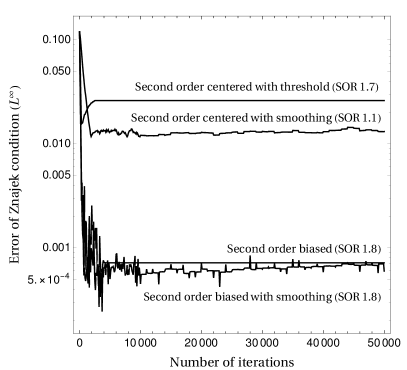
Figure 3: Same problem setup and numerical methodologies as in fig. (2) but here showing the evolution of the $L^{\infty}$ norm of the deviation from the Znajek condition at the horizon. The second order biased stencil provides both fast convergence and evolution towards a configuration fulfilling the Znajek condition.

Our method is based on a finite-difference solution of eq. (11). For that, we discretize all the physical and geometrical quantities in a two dimensional grid. The radial coordinate is compactified according to the transformation $R\left(r\right)=r/\left(r+M\right)$ as introduced by Contopoulos et al. (2013). Radial derivatives are mapped to the $R\left(r\right)$ coordinate by the following transformations:

$$\begin{split}\frac{\partial}{\partial r}=&\>\left[\frac{M}{\left(r+M\right)^{2}}\right]\frac{\partial}{\partial R}\\ \frac{\partial^{2}}{\partial r^{2}}=&\>-\left[\frac{2}{\left(r+M\right)^{3}}\right]\frac{\partial}{\partial R}+\left[\frac{M}{\left(r+M\right)^{2}}\right]^{2}\frac{\partial^{2}}{\partial R^{2}}\end{split}$$ (15)

The computational domain covers the region $[R_{\rm min},R_{\rm max}]\times[0,\theta_{\rm max}]$, where $R_{\rm min}=r_{+}/\left(r_{+}+M\right)$ (i.e., the computational domain extends radially down to the outer event horizon) and $R_{\rm max}$ is specified differently according to the application we seek. The region mapped by the grid may easily be extended to reach all the way to infinity at $R_{\rm max}=1$. In most cases we set $\theta_{\rm max}=\pi/2$ and symmetry with respect to the equatorial plane. Given that the Kerr metric fulfills this property, it is reasonable to search for solutions of the GSE with this symmetry as well. The $\left(R,\theta\right)$ domain is covered by a uniform mesh, where the number of mesh points in the $r$ and $\theta$ directions is $n_{r}$ and $n_{\theta}$, respectively. The discrete values of the magnetic flux $\Psi_{ij}:=\Psi(R(r_{i}),\theta_{j})$ are stored on a two-dimensional array of the same size as the numerical grid, whereas the two remaining functions $\omega\left(\Psi\right)$ and $II^{\prime}\left(\Psi\right)$ are tabulated as a one-to-one map of $\Psi$. For practical purposes, instead of working directly with the function $I(\Psi)$, we use $II^{\prime}(\Psi)$ (cf. Nathanail & Contopoulos, 2014). The latter is related to the former by

$$|I\left(\Psi\right)|=\left[2\int_{0}^{\Psi}II^{\prime}\left(\Psi\right)\right]^{1/2}\;.$$

One should note that the additional arbitrariness of sign induced by the prescribed recovery of the current $I\left(\Psi\right)$ from the function $II^{\prime}\left(\Psi\right)$ should be handled carefully in eq. (12). The numerical solution determining $\Psi$, $\omega\left(\Psi\right)$ and $II^{\prime}(\Psi)$ is obtained using an iterative procedure. In this iteration, the initial values of these functions can be specified freely.

Physically the magnetosphere is divided into three disconnected regions by the two light surfaces of the problem. Mathematically, we shall map this property by solving independently for the scalar function $\Psi$ in each subdomain. The only connection between domains are the regularity conditions at the separatrices among subdomains. Accounting for these facts, the numerical method we propose splits each iteration into three basic blocks of (1) the finite difference solution of the GSE in each of the subdomains, (2) the matching of the solutions across the light surfaces to obtain regular functions and (3) the build-up or update of the functional tables for $\omega(\Psi)$ and $II^{\prime}(\Psi)$. In the following sections, the details of each of these blocks are provided.

3.1 Finite difference solution of the GSE in each subdomain

For the finite difference solution of the GSE in each subdomain we take advantage of the existing computational infrastructure for linear elliptic PDEs used in Adsuara et al. (2016). In order to apply these methods to the non-linear equation at hand, we split the GSE into a term linear in the derivatives of $\Psi$ (right-hand side of eq. 11) and into a part comprising the non-linear source terms (left-hand side of eq. 11). The coefficients of the derivatives as well as the source terms are discretized on the mesh. The GSE (11) can be written in canonical form as

$$\mathcal{C}_{rr}\Psi_{,rr}+\mathcal{C}_{\theta\theta}\Psi_{,\theta\theta}+\mathcal{C}_{r}\Psi_{,r}+\mathcal{C}_{\theta}\Psi_{,\theta}=\mathcal{S},$$ (16)

where $\left(\mathcal{C}_{r},\mathcal{C}_{rr},\mathcal{C}_{\theta},\mathcal{C}_{\theta\theta}\right)$ are the PDE coefficients and $\mathcal{S}$ the sources (left-hand side of eq. 11). We note that the GSE is linear in the higher order derivatives, and that it contains no terms proportional to $\Psi_{,r\theta}$, i.e. $\mathcal{C}_{r\theta}=0$. Following, e.g. Beskin (1997), it is then easy to see from the canonical form of the GSE (eq. 16), that the character of the equation depends on the sign of the discriminant $\mathcal{C}_{r\theta}^{2}-4\mathcal{C}_{rr}\mathcal{C}_{\theta\theta}=-4\mathcal{D}^{2}/\Delta$. Since $\Delta>0$ for $r>r_{+}$ and $\mathcal{D}^{2}>0$ everywhere except at the LSs, the GSE is elliptic. At the LSs ($\mathcal{D}=0$) the character of the equation does not change because of the regularity condition given in eq. 14.

Employing a second order centered finite difference scheme on an equally spaced grid, the discretized form of the GSE reads

$$\begin{split}\mathcal{S}_{i,j}=\>&\Psi_{i-1,j}\left[\frac{\mathcal{C}_{rr}}{\delta r^{2}}-\frac{\mathcal{C}_{r}}{2\delta r}\right]-\Psi_{i,j}\left[\frac{\mathcal{C}_{rr}}{\delta r^{2}}+\frac{\mathcal{C}_{\theta\theta}}{\delta\theta^{2}}\right]\\ &+\Psi_{i+1,j}\left[\frac{\mathcal{C}_{rr}}{\delta r^{2}}+\frac{\mathcal{C}_{r}}{2\delta r}\right]+\>\Psi_{i,j-1}\left[\frac{\mathcal{C}_{\theta\theta}}{\delta\theta^{2}}-\frac{\mathcal{C}_{\theta}}{2\delta\theta}\right]\\ &+\Psi_{i,j+1}\left[\frac{\mathcal{C}_{\theta\theta}}{\delta\theta^{2}}+\frac{\mathcal{C}_{\theta}}{2\delta\theta}\right],\end{split}$$ (17)

where we have dropped subscripts $(i,j)$ of the coefficients $\left(\mathcal{C}_{r},\mathcal{C}_{rr},\mathcal{C}_{\theta},\mathcal{C}_{\theta\theta}\right)$ to avoid cluttering the formulae with subindices. From this discretization, a coefficient matrix is built and used for the iterative relaxation procedure:

$${\cal G}_{S}:={\footnotesize\left(\begin{array}[]{ccccccc}\mathcal{I}^{c}&\mathcal{I}^{u}&0_{n_{r}\times n_{\theta}}&\cdots&\cdots&\cdots&0_{n_{r}\times n_{\theta}}\\ \mathcal{I}^{d}&\mathcal{I}^{c}&\mathcal{I}^{u}&0_{n_{r}\times n_{\theta}}&\cdots&\cdots&0_{n_{r}\times n_{\theta}}\\ 0_{n_{r}\times n_{\theta}}&\mathcal{I}^{d}&\mathcal{I}^{c}&\mathcal{I}^{u}&0_{n_{r}\times n_{\theta}}&\cdots&0_{n_{r}\times n_{\theta}}\\ \vdots&0_{n_{r}\times n_{\theta}}&\ddots&\ddots&\ddots&\vdots&0_{n_{r}\times n_{\theta}}\\ \vdots&\vdots&\ddots&\ddots&\ddots&\ddots&0_{n_{r}\times n_{\theta}}\\ \vdots&\vdots&\vdots&\vdots&\mathcal{I}^{d}&\mathcal{I}^{c}&\mathcal{I}^{u}\\ 0_{n_{r}\times n_{\theta}}&\cdots&\cdots&\cdots&0_{n_{r}\times n_{\theta}}&\mathcal{I}^{d}&\mathcal{I}^{c}\\ \end{array}\right)},$$ (25)

Here, $\mathcal{I}^{c}$, $\mathcal{I}^{u}$ and $\mathcal{I}^{d}$ are matrices with dimensions $n_{r}\times n_{\theta}$, which contain the combinations of coefficients of eq. (17) and $0_{n_{r}\times n_{\theta}}$ is the null matrix with dimensions $n_{r}\times n_{\theta}$.

The numerical elliptic PDE solver is used with an iterative SOR (successive overrelaxation) scheme to find the magnetic flux function $\Psi$. For the complex non-linear system at hand, there is no known optimal relaxation coefficient of the SOR scheme, $\omega_{\rm SOR,opt}$. Thus, we need to choose a value $\omega_{\rm SOR}$ empirically. Numerical experience tells that we shall take a value as close as possible to 2, but not too large such that the iterative scheme diverges. The choice of $\omega_{\rm SOR}$ strongly depends upon the grid properties (e.g., number of grid points, physical domain size) as well as the numerical treatment of the LS.

Both, the grid extension and the discretization stencil have an impact on the diagonal dominance of the resulting coefficient matrices (eq. 25) of the solver. In case of the relativistic GSE (eq. 11), diagonal dominance may be greatly breached at the location of the singular surfaces (cf. condition 13), where the coefficients $\mathcal{C}_{rr}$ and $\mathcal{C}_{\theta\theta}$ vanish. This is mostly due to the fact that points across a separatrix of the computational domain should not be bridged by the finite difference discretization. Stated differently, a derivative on a given computational subdomain must not include values on a different subdomain in its stencil. We point out that this fact was brought about by Camenzind (1987), but in the context of the finite element solution of the GSE. Camenzind (1987) points out, that, as the finite element grid must follow the shape of the light surfaces, the nodal points had to be redistributed iteratively in his numerical method. Turning to our finite difference discretization, we shall see that, e.g., a standard second order centered finite difference approximation of the first derivatives $\Psi^{\prime}$ couples points across LS, rendering a poor convergence (if at all) to the solution. This fact forces us to employ $\omega_{\rm SOR}$ closer to 1, instead to 2. Changing the discretization for the cells around the LS to a left/right biased second order scheme or reducing the approximation to first order of accuracy greatly improves diagonal dominance of the coefficient matrix and, hence, convergence behavior of the numerical solver (see fig. 1).

If not stated otherwise, Dirichlet boundary conditions are imposed along the symmetry axis as well as on the equator in the simulations, where we fix the minimum and maximum values of the potential $\Psi$, respectively. Newman boundary conditions are set up along the radial edges of the computational domain. The latter implies that we set up the derivatives of $\Psi$ normal to the outer horizon at $r=r_{+}$. Note that the value of $\Psi$, or of any other free function of $\Psi$, is not imposed at the outer event horizon. In particular, the so called Znajek condition (Blandford & Znajek, 1977; Znajek, 1977) is not explicitly enforced there.

The iterative solution is stopped when we attain a prescribed reduction of the residual, defined as

$$\mathcal{R}_{\Psi}=\left|\Psi^{(n)}-\Psi^{(n-1)}\right|_{\infty},$$ (26)

where $|.|_{\infty}$ stands for the $L^{\infty}$ norm computed over all the discrete points of our numerical grid (for more details see app. A.1).

3.2 Matching across subdomains

To ensure regularity of the potential $\Psi$ across the light surfaces, we have employed two strategies. First, we perform a cycle consisting of iterative overrelaxations of the GSE interleaved with numerical resets of the values of $\Psi$ developed at the light surfaces. The mentioned cycle starts computing a series of iterations of the solution on each of the three subdomains independently. This brings a mismatch between solutions across subdomains. The most severe mismatch happens at the ILS, where numerical artifacts develop. In order to smooth out the solution, we build high-order Lagrange interpolation polynomials in the radial direction for $\Psi$. These polynomials have a stencil centered around the light surfaces on each different discrete value of $\theta_{j}$ ($j=1,\ldots,n_{\theta}$). Thus, they encompass points in two different computational domains. At the radial location of the light surfaces we obtain an smooth interpolant of $\Psi$, which replaces the numerical values (artifacts) developed there in the course of the iterative solution. We repeat the whole cycle until convergence is reached. This first strategy follows from Nathanail & Contopoulos (2014), but we employ higher-order polynomial interpolants for $\Psi$ ($5^{th}$ order Lagrangian interpolation, instead of just taking for $\Psi$ the average between its values on both sides of a light surface - cf. eq. (15) of Nathanail & Contopoulos 2014).

The second strategy consists in producing a central, second order finite difference discretization in all points of the computational domain except close to the light surfaces. There we switch to a (left/right) biased, second order, finite difference discretization of the first derivatives of the GSE. This procedure notably reduces the coupling between different physical domains. However, since the light surfaces are not spherical, some unwanted couplings may develop due to the discretization of angular derivatives. As a result of the biased discretization the coefficient matrix of the linear system to be solved (eq. 25) improves its diagonal dominance. The improved diagonal dominance results in a faster convergence of the method than when no biased discretizations are employed (as we shall see in sec. 4). In fig. 1 we clearly see that a second order biased discretization around the light surfaces works better if no smoothing is applied to $\Psi$. Indeed, with the use of a biased discretization the need of any smoothing of the solution at the light surfaces disappears and we do not apply it. This matching strategy follows the general guidelines devised by Leveque & Li (1994) for the treatment of immersed boundaries in second-order elliptic equations.

A third strategy has also been tested, namely, we employ a second order centered discretization everywhere, but at the light surfaces we use a threshold for the coefficients $\mathcal{C}_{rr}$ and $\mathcal{C}_{\theta\theta}$ ensuring diagonal dominance of the matrix of the system (eq. 25). Note that $\mathcal{C}_{rr}=\mathcal{C}_{\theta\theta}=0$ on the light surfaces. Thus, the proposed recipe consists of replacing the aforementioned coefficients by

$$\mathcal{C}_{rr} =\textrm{sign}(\mathcal{C}_{rr})\times\max{(|\mathcal{C}_{rr}|,\epsilon)},$$

$$\mathcal{C}_{\theta\theta} =\textrm{sign}(\mathcal{C}_{\theta\theta})\times\max{(|\mathcal{C}_{\theta\theta}|,\epsilon)},$$

with $\epsilon\sim 10^{-5}$. As in the case of the second strategy, the thresholding of the coefficients of the second order derivatives renders unnecessary any smoothing procedure at the light surfaces. Fig. 1 shows that the second and third strategies yield a quite similar reduction of the residual with the number of iterations.

In fig. 2 we show the evolution of the residual with the number of iterations in the solver, again, for different matching strategies. Differently from fig. 1, in this case we include the whole space time ($r_{\rm max}=\infty$). Regardless of whether we set the outer boundary conditions at finite or infinite distance, the qualitative conclusion is the same. Namely, either thresholding the coefficients of the second order derivatives, or employing a biased discretization close to the light surfaces brings a much larger reduction (by roughly 9 orders of magnitude) than smoothing the solution across the light surfaces. Furthermore, smoothing procedures are unable to reduce substantially the residual for coarse discretizations. The results shown in figs. 2 and 1 also hold for higher resolutions.

Since the second strategy presented in this section (left/right biased stencils) does not depend on any additional tunable parameter and since it yields a reduction of the residual comparable to the case of using thresholding, we will use it as our default method to match the solution across different subdomains.

3.3 Update of the potential functions

The potential functions $\omega\left(\Psi\right)$ and/or $II^{\prime}\left(\Psi\right)$ could be updated every time the magnetic flux $\Psi$ changes in the course of the iterative relaxation sketched in sec. 3.1. In practice, it is unnecessary to update $\omega\left(\Psi\right)$ and $II^{\prime}\left(\Psi\right)$ with this frequency. Instead, the mentioned update is performed after $n_{\rm u}\geq 1$ iterations. The choice of $n_{\rm u}$ comes as a tradeoff between accuracy and computational time.

The update of both functions simultaneously (see Contopoulos et al., 2013), as well as with one of them fixed (cf. Uzdensky, 2004) to an initially specified value are equally possible in our scheme. For convergence testing we have considered both cases, i.e., the relaxation of either $\omega\left(\Psi\right)$ (not shown here) or $II^{\prime}\left(\Psi\right)$ (fig. 1) and of both functions simultaneously (fig. 2). A cautionary note must be added here. The number of light surfaces in the computational domain determines whether one or none of the potential functions can be arbitrarily set up. More precisely, the number of freely specifiable potential functions equals two minus the number of light surfaces in the domain. For instance, if the OLS radius is sufficiently large (e.g., when $a\rightarrow 0$), the outermost radial computational domain may be set inside of the OLS for numerical convenience. In this case, we are allowed to freely specify either $\omega(\Psi)$ or $I(\Psi)$. This is the simplification we employ to obtain the results shown in fig. 1. Note, however, that if the numerical domain contains both LS, there is no freedom to set the potential functions. They must be recovered from eq. (27) applied both at the ILS and the OLS. The convergence properties of the latter case can be seen in fig. 2. In view of the results, the global convergence properties of the algorithm are not sensitively dependent on the choice of updating only one or both potential functions.

The updates of the potential functions are conducted by minimizing the error of eq. (14) after determining the exact radial position of the LS and the corresponding interpolated quantities. More specifically, we define the residual at the LS as

$$\begin{split}\mathcal{R}_{\rm LC}=&\left|\>4\frac{\Sigma}{\Delta}II^{\prime}-\right.\left(\frac{A_{,r}}{A}+\frac{\Sigma_{,r}}{\Sigma}\right)\Psi_{,r}-\frac{2Mr}{\Delta\Sigma}\frac{\Sigma_{,\theta}}{\Sigma}\Psi_{,\theta}\\ &-\frac{4Mar\omega\sin^{2}\theta}{\Delta\Sigma}\frac{A_{,\theta}}{A}\Psi_{,\theta}\\ &-\left(2\>\frac{\cos\theta}{\sin\theta}+\frac{A_{,\theta}}{A}-\frac{\Sigma_{,\theta}}{\Sigma}\right)A\omega\left(\omega-\frac{4Mar}{A}\right)\frac{\sin^{2}\theta}{\Delta\Sigma}\Psi_{,\theta}\\ &+\left(\frac{2Mr}{\Sigma}-\frac{4Mar\omega\sin^{2}\theta}{\Sigma}\right)\left(\frac{A_{,r}}{A}-\frac{1}{r}\right)\Psi_{,r}\\ &\left.-\frac{\sin^{2}\theta}{\Sigma\Delta}\left(A\omega-2Mar\right)\left(\Delta\>\omega_{,r}\>\Psi_{,r}+\omega_{,\theta}\>\Psi_{,\theta}\right)\>\right|,\end{split}$$ (27)

and attempt to minimize it (see also the convergence criterion in app. A.1). The process of minimizing $R_{\rm LC}$ depends on whether we fix one of the two free potential functions (and which one of them) or if we leave both to be numerically obtained from the reduced GSE (eq. 14) applied at both LS. Independent of the fixing or relaxing of the function $\omega(\Psi)$ (see below), the functional update of $II^{\prime}$ is achieved in a straightforward manner by substitution of $\omega$ and $\omega^{\prime}$ into the right-hand side of expression (eq. 14) at the LS. If we do not initially specify the rotational profile and keep it throughout the iterative solution, then we need to provide initial guesses $\omega_{0}$ and $\omega^{\prime}_{0}$ for $\omega$ and its derivative, respectively. We note that every time $\omega$ is changed, the location of the LS (eq. 13) changes. The practical procedure consists on taking a set of a few thousands of values $\omega_{0}$ and $\omega^{\prime}_{0}$ uniformly selected in the intervals $[\omega(\Psi)-\xi,\omega(\Psi)+\xi]$ (throughout the shown tests we use $\xi=0.15$) and for each of these values we compute $R_{\rm LC}$ (eq. 27). Among all these pairs of values $\omega_{0}$ and $\omega^{\prime}_{0}$ we pick the one which minimizes $R_{\rm LC}$.

Optimal and stable results require an exact localization of the LS positions. Since we employ a finite difference method, the spatial discretization determines the numerical accuracy with which the singular surfaces are resolved. However, for practical grid resolutions, it is necessary to exceed the accuracy of the numerical grid in order to achieve high accuracy in resolving eq. (27). Once it is detected that a given numerical cell between grid points, namely, bounding the region $[r_{i},r_{i+1}]\times[\theta_{j},\theta_{j+1}]$, is traversed by a LS, our algorithm improves the accuracy of its localization using either Lagrangian interpolation polynomials or bicubic spline interpolation if a higher resolution is desired. In the presented solutions, especially for lower values of the BH spin parameter $a$, the numerical grid is refined before every update of the potential functions and bicubic spline interpolation is used to determine the quantities at the respective LS. For small values of $\theta$ (i.e., the first few zones at the $\theta_{min}$ boundary), we approximate the potential $\Psi$ by the initially guessed function in order to avoid numerical artifacts due to the small distance between the ILS and the event horizon (as suggested by Contopoulos et al., 2013).

The functions $\omega_{\rm ns}(\Psi)$ and $II^{\prime}_{\rm ns}(\Psi)$ obtained with the previous procedures tend to be non-smooth. This lack of smoothness degrades the convergence properties of the finite difference solution. Thus, we replace $\omega_{\rm ns}$ and $II^{\prime}_{\rm ns}$ by smooth cubic spline interpolants of the latter functions (cf. Contopoulos et al., 2013; Nathanail & Contopoulos, 2014). For that, we pick a sample of $n_{\rm int}$ values of both $\omega_{\rm ns}$ and $II^{\prime}_{\rm ns}$ as nodal points for the cubic spline interpolation. The number of nodal points may be chosen in the algorithm setup and may influence the accuracy of the solution (the presented runs employed $n_{\rm int,\omega}=5$ and $n_{\rm int,II^{\prime}}=10$). Especially for the first relaxation steps a lower order of $n_{\rm int,\omega}$ and $n_{\rm int,II^{\prime}}$ may be beneficial in order to prevent undesired oscillations. The presented procedure has been tested as well with $n_{\rm int,\omega}=10$ and $n_{\rm int,II^{\prime}}=20$ differing in the rate of initial convergence without noticeable changes to the relaxed solution.

Uzdensky (2004) has applied the update of the current function employing eq. (14) in order to find the field configuration of a central engine with the field line angular velocity fixed by the disk’s rotation. With the suggested methodology for the updating of the potential functions, we generalize his approach by allowing the fixing of either potential function.

3.4 The Znajek condition at $r_{+}$

A key ingredient of the derivation of an outflowing energy and a process efficiency measure at the horizon in Blandford & Znajek (1977) is the so called Znajek boundary condition. Historically by Weber & Davis (1967) and context specific by Znajek (1977), the question for asymptotic fields in magnetohydrodynamics was posed. Requiring finite field and potential quantities at the horizon, the so called Znajek ‘boundary condition’ sets a link among the angular derivative of $\Psi$ and the potential functions $I(\Psi)$ and $\omega(\Psi)$ at the outer BH horizon:

$$I_{Z}\left(\Psi\right)=-\frac{Mr_{+}\sin\theta}{r_{+}^{2}+a^{2}\cos^{2}\theta}\left[\Omega-\omega\left(\Psi\right)\right]\Psi_{,\theta}$$ (28)

Despite its original purpose as a boundary condition, recent studies suggest that eq. (28) is a regularity condition which is automatically satisfied in numerical procedures demanding smoothness at the LS (Komissarov, 2004; Nathanail & Contopoulos, 2014). Observing the behavior of the $L^{\infty}$ norm of the difference between the function $I\left(\Psi\right)$ and $I_{Z}(\Psi)$ for different stencils at $r=r_{+}$, we are able to confirm the status of eq. (28) as a regularity condition, which is automatically fulfilled throughout the numerically iterative procedure with the imposed regularity at the LS (see fig. 3). As we can see from that figure, the reduction of the error in the preservation of the Znajek condition happens for all the matching strategies presented in sec. 3.2. However, the error level in the preservation of such condition is some orders of magnitude smaller when employing a biased discretization of the second order radial derivatives, regardless of the application of any smoothing procedure for $\Psi$ at the light surfaces.

The initial error depends on the chosen spin factor $a$ and becomes greater for BHs which are close to maximally rotating. The deviations between the numerical solution and the Znajek condition are dominated by the matching point between the BH horizon and the equator as well as close to the axis of rotation, where an approximation of $\Psi$ becomes necessary (cf. Contopoulos et al., 2013).

4 Numerical Results

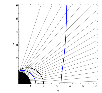
Figure 4: Distribution of the magnetic flux $\Psi$ in the vicinity of a fast rotating ($a_{*}=0.9999$) BH. In order to reach the configuration displayed, the GSE has been solved numerically until the convergence criterion (61) has been reached in a physical domain $[r_{+},\infty]\times[0,90^{\circ}]$, covered with a numerical grid $\left[n_{r}\times n_{\theta}\right]=\left[200\times 64\right]$. The location of the ergosphere is represented by the black line, the two LS are drawn as blue lines. Magnetic flux configurations have been studied for various spin parameters, some of which are visualized in appendix A.1.

4.1 Split monopole configurations

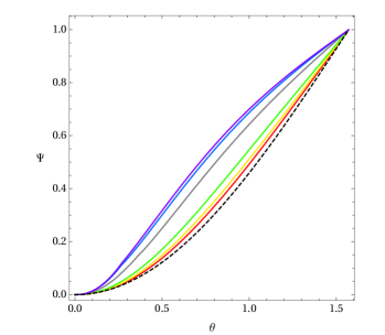
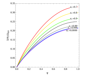
Figure 5: Comparison of split-monopole solutions to the GSE for different spin parameters $a_{*}=\left\{0.7,0.8,0.9,0.99,0.999,0.9999\right\}$ in a physical domain $[r_{+},\infty]\times[0,90^{\circ}]$, covered with a numerical grid $\left[n_{r}\times n_{\theta}\right]=\left[200\times 64\right]$. Top: Angular distribution of the magnetic flux at the location of the inner light surface. The dashed line represents the initial values of the potential $\Psi_{0}$. Middle: Distribution of $\omega\left(\Psi\right)$ after convergence. Bottom: Distribution of $I\left(\Psi\right)$ after convergence.

The first test for the numerical solution of the GSE is the split-monopole (cf. Ghosh, 2000), which has also been discussed by many authors (e.g., Komissarov 2004; Contopoulos et al. 2013; Nathanail & Contopoulos 2014). In the limit of a slowly rotating black hole, the split-monopole matches the flat spacetime solution of Michel (1973) at large radii, while at the same time it satisfies the so called Znajek condition (eq. 28) at the event horizon. Admittedly, this solution is unphysical since in astrophysical conditions the magnetic field threading the horizon of a BH is supported by the electric currents in an accretion disc (c.f. Blandford & Znajek, 1977; Komissarov, 2004). Nevertheless, it is likely the simplest configuration that allows one to demonstrate the extraction of energy through the BZ mechanism. The initial guess for the potential $\Psi$ corresponds to a homogeneous solution of eq. (11) in the case of $a=0$ (also called the Schwarzschild monopole, e.g., Ghosh 2000):

$$\Psi_{0}\left(r,\theta\right)=1-\cos\theta,$$ (29)

where the maximum value of $\Psi$ has been normalized to 1. In order to set the initial functional dependence of $\omega(\Psi)$ and $I(\Psi)$, we adopt the field line angular velocity as being half the BH angular velocity $\omega=\Omega_{\rm\text{\tiny BH}}/2$ (Blandford & Znajek, 1977). For the currents we employ the analytical solution of the pulsar magnetosphere. More specifically we set:

$$\omega_{0}\left(\Psi\right)= \frac{1}{2}\frac{a}{r_{+}^{2}+a^{2}}$$

$$I_{0}\left(\Psi\right)= -\frac{1}{\mbox{{2}}}\omega\left(\Psi\right)\Psi\left(2-\Psi\right)$$

for $\Psi_{\rm min}\leq\Psi\leq\Psi_{\rm max}$, where $\Psi_{\rm min}:=0$ and $\Psi_{\rm max}:=1$ are given by the potential on the (Dirichlet) boundaries at the axis of rotation ($\theta=0$) and the equator ($\theta=\pi/2$), respectively (eq. 29). As stated before, Newman boundary conditions are set up along the radial edges of the computational domain (i.e., at $r=r_{+}$ and at $r=r_{\rm max}$). Using eq. (12) the corresponding initial magnetic fields are

$$B^{r}(r,\theta)= \>\frac{\sin\theta}{2\pi\sqrt{\gamma}},$$ (30)

$$B^{\theta}(r,\theta)= \>0,$$ (31)

$$B^{\phi}(r,\theta)= \>\frac{a}{4(r_{+}^{2}+a^{2})}\sqrt{\frac{\Sigma}{A\Delta}}.$$ (32)

Figure 4 shows the topology of the magnetic flux $\Psi$ computed solving numerically the GSE until our convergence criterion (eq. 61) is reached. We display the case of a nearly maximally rotating BH ($a_{*}=0.9999$) in fig. 4. The isocontours of $\Psi$ pass smoothly through both LS (displayed with thick blue lines). A comparison of solutions to the GSE for different spin parameters is shown in fig. 5.

In all tests where $\omega$ and $I$ are let to relax from their initial values, the error measures $\mathcal{R}_{\Psi}$ and $\mathcal{R}_{\rm LC}$ can be reduced substantially after a sufficiently large number of iterative steps. This demonstrates that our method is robust and converges to a smooth, numerically stable solution. For this to happen, a number of technical comments are crucial at this point. First, we find convergence to a smooth solution if we set a double convergence criterion both on $\mathcal{R}_{\Psi}$ and $\mathcal{R}_{\rm LC}$ (see app. A.1). In contrast to Nathanail & Contopoulos (2014), if we restrict our solution procedure to relax the initial set up for 3000-4000 iterations, one does not find a steady state solution. As shown in the bottom panels of fig. 1 of Nathanail & Contopoulos (2014) the solution displays kinks close to the ILS. Many more iterations are necessary to qualify the numerical solution as a ‘steady state’ (for details, see app. A).

4.2 Paraboloidal configurations

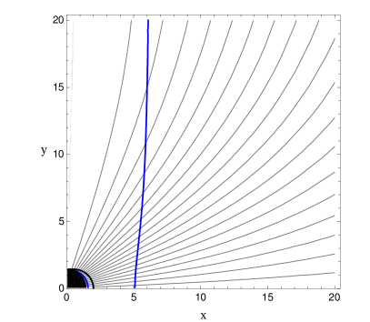
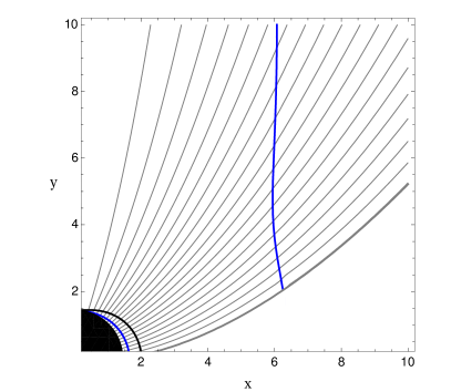
Figure 6: Distribution of the magnetic flux $\Psi$ in the vicinity of a fast rotating $a_{*}=0.9$ BH employing appropriate boundary conditions for paraboloidal confinement (cf. sec. 4.2) in a physical domain $[r_{+},100]\times[0,90^{\circ}]$, covered with a numerical grid $\left[n_{r}\times n_{\theta}\right]=\left[200\times 64\right]$. Top: Far boundary according to Fendt (1997). Bottom: Paraboloidal confinement following the Nathanail & Contopoulos (2014) setup ($r_{0}=10$).

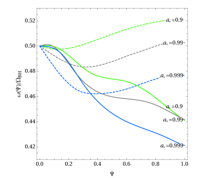
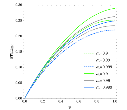
Figure 7: Final distributions (after convergence is reached) of the scalar functions $\omega\left(\Psi\right)$ (top panel) and $I\left(\Psi\right)$ (bottom panel) in the vicinity of fast rotating BHs of different spin parameters $a_{*}=\left\{0.9,0.99,0.999\right\}$ embedded in paraboloidal magnetic field magnetosphere (cf. sec. 4.2). The physical domain $[r_{+},100]\times[0,90^{\circ}]$ is covered with a numerical grid $\left[n_{r}\times n_{\theta}\right]=\left[200\times 64\right]$. The relaxed solution of the Fendt (1997) approach is represented with dashed lines, the Nathanail & Contopoulos (2014) strategy by solid lines.

Collimated magnetospheres are an important ingredient of jet outflows from compact objects and may be found, e.g., in the parabolically shaped solutions to the GSE which have been studied by, e.g., Fendt (1997) and Nathanail & Contopoulos (2014). Fendt (1997) considers an asymptotically cylindrical shape of the magnetic field and suggests to set up the outer radial boundary at $r_{\rm max}$ according to

$$\Psi_{\rm out}(x)=\frac{1}{b}\ln\left(1+\frac{x^{2}}{d^{2}}\right),$$ (33)

where the constants $d$ and $b$ determine the degree of collimation and $x=r\times\sin\theta$. Fendt (1997) adapts his finite element computational domain to provide a parabolically shaped outer jet boundary. Indeed, we have considered setting up Fendt’s boundaries at radial infinity, resulting into a final solution which resembles that of a split monopole (i.e., effectively unconfined). Bringing condition (33) to a finite distance, solutions with a degree of confinement larger than the split monopole case are possible. For instance, in fig. 6 (upper panel) we show the solution for $\Psi$ when setting the Dirichlet boundary condition (33) at $r_{\rm max}=100$ for values of the confinement parameters $b=9.2$, $d=1.0$.

The numerical relaxation proceeds without obstacles and ultimately yields solutions, which show higher confinement at the OLS (comparing to the split-monopole solutions in sec. 4.1). It should be noted, that an appropriate choice of boundary conditions at $r_{\rm max}$ is crucial for the relaxation towards a paraboloidal setup. Using a parabolic topology as initial guess but with Newman boundary conditions (zero derivative) at $r_{\rm max}$ and no further induced confinement will result in a split-monopole solution.

However, setting Fendt’s condition at finite distance is artificial and difficult to justify in astrophysical BH magnetospheres. As an alternative, Nathanail & Contopoulos (2014) suggest to solve the GSE for a confined parabolic setup limiting the computational domain to a region $0\leq\Theta\leq 1$, where

$$\Theta\left(r,\theta\right)=\frac{\theta}{\theta_{\rm wall}\left(r\right)},$$

and $\theta_{\rm wall}\left(r\right)$ describes a paraboloidal wall according to the function

$$1-\cos\theta_{\rm wall}=\left(\frac{r+r_{0}}{r_{+}+r_{0}}\right)^{-\nu}.$$ (34)

Here, $r_{0}$ and $\nu$ are parameters determining the degree of confinement of the parabolic boundary wall, e.g., a choice of $r_{0}=\infty$ or $\nu=0$ reduces to the split monopole initial guess in eq. (29). Employing $\Theta\left(r,\theta\right)$ to define the angular coordinate (c.f., Nathanail & Contopoulos, 2014), allows us to use the numerical solver as in previous examples without the need for excising regions of the computational domain in the vicinity of the equatorial plane in order to ensure the paraboloidal character of the solution. Employing the function

$$\theta\left(r,\Theta\right)=\Theta\times\theta_{\rm wall}\left(r\right),$$

where $\Theta\in\left[0,1\right]$, as well as the following coordinate changes in the angular derivatives (cf. eq. (15) for the radial derivatives)

$$\begin{split}\frac{\partial}{\partial\theta}=&\>\frac{1}{\theta_{\rm wall}\left(r\right)}\frac{\partial}{\partial\Theta}\\ \frac{\partial^{2}}{\partial\theta^{2}}=&\>\left(\frac{1}{\theta_{\rm wall}\left(r\right)}\right)^{2}\frac{\partial^{2}}{\partial\Theta^{2}},\end{split}$$

no further changes to the update and LS routines are necessary. After setting up an initial guess for the potential according to (following Nathanail & Contopoulos, 2014)

$$\Psi\left(r,\theta\right)=\Psi_{\rm max}\left(\frac{r+r_{0}}{r_{+}+r_{0}}\right)^{\nu}\left(1-\cos\theta\right),$$ (35)

with $\Psi_{\rm max}=1$ for simplicity, as well as $\omega\left(\Psi\right)$ and $II^{\prime}\left(\Psi\right)$ like in sec. 4.1, the numerical solution converges without obstacles. We observe, however, that with larger confinement (i.e., lower values of $r_{0}$), the kinks at the OLS become stronger, especially close to the equatorial plane. The growing artifacts may be reduced with lower relaxation factors in the SOR routines. The presented example (fig. 6 bottom panel) shows the converged solution (demanding condition 61) for $\omega_{\rm SOR}=1.0$ after $42.740$ iterations. The solid lines in fig. 7 display the distributions of $\omega\left(\Psi\right)$ and $I\left(\Psi\right)$ after convergence is reached employing the set up of Nathanail & Contopoulos (2014). For comparison, we also display (with dashed lines) the final distributions of $\omega\left(\Psi\right)$ and $I\left(\Psi\right)$ employing the paraboloidal problem set up of Fendt (1997). From the top panel of fig. 7, it is evident that the latter set up tends to produce solutions with faster rotating field lines, not only in the equatorial plane (corresponding to a value $\Psi=1$), but at almost every other latitude in the domain ($\Psi=0$ corresponds to the axis of symmetry).

4.3 Vertical field configurations

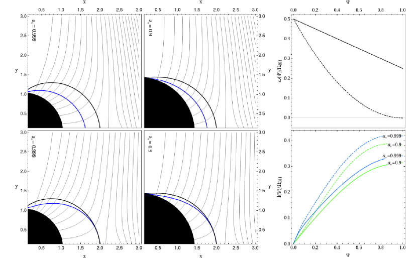
Figure 8: Distribution of $\Psi$ (left and central columns), of $\omega\left(\Psi\right)$ (top right panel) and of $I\left(\Psi\right)$ (bottom right panel) in the vicinity of fast rotating BHs of different spin parameters $a_{*}=\left\{0.9,0.999\right\}$ embedded in a vertical magnetic field (cf. sec. 4.3). The physical domain $[r_{+},100]\times[0,90^{\circ}]$ is covered with a numerical grid $\left[n_{r}\times n_{\theta}\right]=\left[200\times 200\right]$. In the top right panel we depict the (fixed) fieldline profiles of $\omega\left(\Psi\right)$ given by eq. (37) (solid line) and eq. (36) (dashed line). The upper left and middle panels show the spatial distribution of $\Psi$ corresponding to the imposed profile of $\omega\left(\Psi\right)$ given by eq. (37). The bottom left and middle panels show the spatial distribution of $\Psi$ corresponding to $\omega\left(\Psi\right)$ given by eq. (36). The relaxed values of $I\left(\Psi\right)$ corresponding to the two (fixed) distributions of $\omega\left(\Psi\right)$ are shown on the bottom right panel (using the same line styles as in the upper right panel).

Another well studied exemplary fieldline configuration is the embedding of a BH into a vertical magnetic field. Originally considered by Wald (1974) for the electrovacuum limit, it has since been studied in dynamical evolutions (see, e.g., Komissarov, 2004; Komissarov & McKinney, 2007; Palenzuela et al., 2010) as well as with a focus on the BH "Meissner effect" (Komissarov & McKinney, 2007; Nathanail & Contopoulos, 2014), or on the uniqueness of the numerical solutions (Pan et al., 2017). The case of vertical fieldlines opens up the possibility of fieldlines crossing only the ILS (for a detailed discussion, see also Nathanail & Contopoulos, 2014) and, hence, the freedom of fixing either $\omega\left(\Psi\right)$ or $I\left(\Psi\right)$ throughout the relaxation procedure (cf. sec. 3.3).

We employ a Dirichlet boundary at $\theta=0$, as we have done in sec. 4.1. In order to fill up the initial magnetic field configuration we divide the computational domain into three regions. The first region is the spherical shell surrounding the BH and extending slightly beyond the ergosphere defined by

$$r<1.25\times r^{*}_{+}(\pi/2)\equiv r_{0}\>,$$

where we employ the split monopole potential $\Psi_{0}$ (eq. 29). The second region extends beyond the previous spherical shell up to infinity in the vertical direction, i.e. enclosing the region

$$r_{0}\leq r<r\times\sin\theta\>,$$

where the isolines of $\Psi$ are vertical and their values correspond to

$$\Psi(r,\theta)=\Psi_{0}\left(r,\arcsin\left(\frac{r\times\sin\theta}{r_{0}}\right)\right)\>.$$

Finally, in the third region, defined by $r\times\sin\theta>r_{0}$, we use

$$\Psi\left(r,\theta\right)=\left(\frac{r\times\sin\theta}{r_{0}}\right)^{2}.$$

We apply the following Dirichlet boundary condition at the equator:

$$\Psi\left(r,\theta=\frac{\pi}{2}\right)=\left\{\begin{array}[]{cc}1.0&\text{if }r<r_{0}\\[10.00002pt] \displaystyle\left(\frac{r}{r_{0}}\right)^{2}&\text{otherwise}\end{array}\right.$$

Newman boundary conditions are set up along the radial edges of the computational domain (i.e. at $r=r_{+}$ and at $r=r_{\rm max}$). Following Nathanail & Contopoulos (2014), we initiate the fieldline angular velocity to one of the two functions

$$\omega\left(\Psi\right) =\frac{\Omega_{\rm\text{\tiny BH}}}{2}\times\left(1-\Psi\right)^{2}$$ (36)

$$\omega\left(\Psi\right) =\>\frac{\Omega_{\rm\text{\tiny BH}}}{2}\times\left(1-\frac{\Psi}{2}\right),$$ (37)

for $\Psi_{\rm min}\leq\Psi\leq\Psi_{\rm max}$, where $\Psi_{\rm min}:=0$ and $\Psi_{\rm max}:=1$, and zero otherwise. This choice of $\omega\left(\Psi\right)$ pushes the OLS to infinity and allows us to update only the current function $I\left(\Psi\right)$ throughout the numerical relaxation. By the construction of the boundary conditions, eq. (36) ensures that the ILS touches the outer ergosphere $r_{+}^{*}$ at the equator, while eq. (37) provides an ILS well inside the outer ergosphere $r_{+}^{*}$.

The initial values employed for the numerical algorithm and the equatorial boundary conditions slightly differ from those employed in Nathanail & Contopoulos (2014), but they provide smooth profiles of the ILS and no glitches in the field lines in the region enclosed in between of the ILS and the outer ergosphere (see the left and middle panels of fig. 8). These results can be compared with the ones presented by Nathanail & Contopoulos (2014; fig. 3) or by Pan et al. (2017; fig. 1). The fact that the configurations we find are slightly different to those of the previous works is simply a consequence of the different boundary conditions employed, and not necessarily related to a lack of uniqueness of the GSE solution (see Pan et al., 2017, and Sec. 6 for a discussion of the uniqueness of the GSE solution for the vertical magnetic field configuration).

We have further explored the influence of the equatorial boundary conditions by setting up an approximately vertical magnetic field employing a paraboloidal setup as discussed in sec. 4.2, e.g. by using the parameters $r_{0}=0$, and $\nu=2$ in eqs. (34) and (35). The relaxed solutions are as smooth as those obtained with the previous initialization for $\Psi$ and the corresponding equatorial boundary conditions. In none of the two cases the Meissner effect is observed, in full agreement with the findings of e.g. Nathanail & Contopoulos (2014) or Pan & Yu (2016).

4.4 BH-disk models

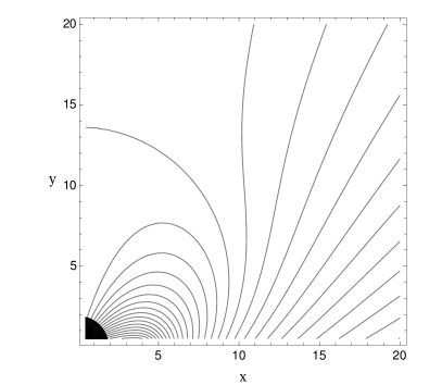
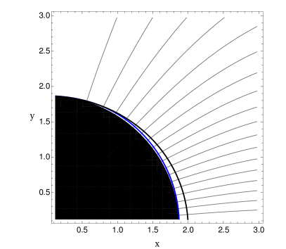
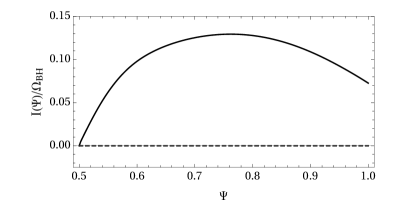
Figure 9: BH-disk model following the setup by Uzdensky (2005) after the relaxation procedure ($a_{*}=0.5,[r_{+},{100}]\times[0,90^{\circ}],\left[n_{r}\times n_{\theta}\right]=\left[200\times 200\right]$). The fieldlines connecting the BH to the disk rotate with Keplerian velocity. The open fieldlines are free of rotation and current. Top/Middle: Global structure and zoom of the inner region showing in detail the location of the ILS (blue line) in between of the ergosphere (thick black line) and the outer event horizon. Bottom: Distribution of $I\left(\Psi\right)$ after convergence. The dashed line represents the initial configuration $I_{0}\left(\Psi\right)=0$.

Uzdensky (2005) suggests the setup of a BH-disk system via a suitable choice of boundary conditions in the numerical solution of the GSE. In these configurations, field lines threading the BH horizon connect to the equatorial plane and rotate with Keplerian velocity. Following Uzdensky (2005), the boundary along the axis of rotation and the equatorial plane are set up as follows:

$$\Psi\left(\theta=0\right) =\Psi_{\rm s}$$

$$\Psi\left(r>r_{\text{in}},\theta=\frac{\pi}{2}\right) =\Psi_{\rm d}\left(x\right)$$

$$\Psi\left(r\leq r_{\text{in}},\theta=\frac{\pi}{2}\right) =\Psi_{\rm max}.$$

Here, $r_{\text{in}}=r_{\text{ISCO}}\left(a\right)$ is the radial location of the innermost circular orbit as a function of $a$. $\Psi_{\rm s}$ fixes the value of the separatrix between open field lines and field lines linking the BH to the disk. Their potential is connected to the disk radius by

$$\Psi_{\rm d}\left(r\right)=\Psi_{\text{max}}\left(\frac{r_{\text{in}}}{r}\right).$$

Homogeneous Neumann boundary conditions are set at the outer event horizon,

$$\Psi_{,r}\left(r=r_{+}\right)=0.$$

We find that it is necessary to fix the boundary at $r_{\rm max}$ to a predefined shape function similar to the paraboloidal case presented in sec. 4.2:

$$\Psi\left(r=r_{\rm max}\right)=\Psi_{\rm s}+\left[\Psi_{\rm d}\left(r\right)-\Psi_{\rm s}\right]\left(1-\cos\theta\right).$$

As for the field line angular velocity $\omega$, it is assumed that the field lines connected to the BH rotate with the Keplerian angular velocity $\Omega_{\rm K}$ of the disk,

$$\Omega_{\rm K}\left(r\right)=\frac{\sqrt{M}}{r^{3/2}+a\sqrt{M}},$$

and do not rotate for $\Psi<\Psi_{\rm s}$, namely,

$$\omega\left(\Psi\right)=\left\{\begin{array}[]{cc}0&\text{if }\Psi<\Psi_{\rm s}\\[10.00002pt] \Omega_{\rm K}\left[r_{0}\left(\Psi\right)\right]\displaystyle\tanh^{2}\left(5\frac{\Psi-\Psi_{\rm s}}{\Psi_{\text{tot}}-\Psi_{\rm s}}\right)&\text{otherwise}\end{array}\right.$$

where $r_{0}$ represents the footpoint of a given field line with potential $\Psi$ on the disk.

Following Uzdensky (2005), we use a grid of $\left[n_{r}\times n_{\theta}\right]=\left[200\times 200\right]$ numerical nodes. However, relatively small values of $a$ let the ILS approach the outer BH event horizon $r_{+}$, rendering insufficient the previous radial grid resolution (see the LS position in the mid panel of fig. 9). Therefore, we choose to adapt the radial coordinate for the discretization to the function $R_{\rm min}=r_{+}/\left(r_{+}+10M\right)$, and refine the grid increasing by a factor of 20 the number of nodes in the radial direction whenever we update the potential functions $I\left(\Psi\right)$ and $\omega\left(\Psi\right)$, e.g. we employ $\left[n_{r}\times n_{\theta}\right]=\left[4000\times 200\right]$ for $a_{*}=0.5$ in order to ensure sufficient data points around the ILS. As $I\left(\Psi\right)=0$ and $\omega\left(\Psi\right)=0$ for $\Psi<\Psi_{\rm s}$, the OLS is pushed to infinity and the magnetosphere is current-free along the open field lines. The numerical relaxation proceeds smoothly towards a converged equilibrium solution (see fig. 9), which closely matches that found by Uzdensky (2005).

5 Power of the BZ process

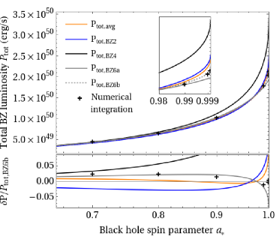
Figure 10: Comparison of the power of split-monopole solutions to the GSE in a physical domain $[r_{+},\infty]\times[0,90^{\circ}]$, covered with a numerical grid $\left[n_{r}\times n_{\theta}\right]=\left[200\times 64\right]$. The figure shows the total process power derived for different BH spin parameters of a $1M_{\odot}$ BH computed using the direct numerical evaluation of eq. (39) (black crosses), the approximated value of Lee et al. (eq. 41; orange line), as well as the second order (blue line) and 6th order (gray line) approximations of the BZ power as suggested by Tchekhovskoy et al. (2010). The 6th order approximation (eq. 53) fitted to the numerical data (following eq. 42) is denoted by the dotted line. The extremal spin segment is magnified within the plot.

Approximation	$P_{\rm tot,avg}$	$P_{\rm tot,BZ2}$	$P_{\rm tot,BZ4}$	$P_{\rm tot,BZ6a}$
RMS error	9.23	13.21	50.49	7.19

Table 1: RMS error of the different approximations computed for the total BZ power presented in fig. 10. The results are normalized to the RMS of the 6th order approximation computed using eq. (53) and the fit parameters $b_{1}=0.81$ and $b_{2}=-5.61$ (BZ6b).

The question of whether relativistic jets can be formed extracting the reducible energy of a rotating BH has been recurrently investigated in the last decades, both in the context of AGN jets (e.g. McKinney, 2005; Hawley & Krolik, 2006; Komissarov & McKinney, 2007; Reynolds et al., 2006; Garofalo, 2009; Palenzuela et al., 2011), as well as in the context of gamma-ray bursts (e.g. Komissarov & Barkov, 2009; Nagataki, 2009; Tchekhovskoy & Giannios, 2015; Nathanail et al., 2016). In this section, we employ the obtained solutions of the GSE in the split monopole magnetic field configuration to provide some analytic estimates of the total BZ power, as well as its distribution with latitude.

We compute the total BZ power (cf. also, Thorne et al., 1986; Lee et al., 2000; Uzdensky, 2004; McKinney & Gammie, 2004; Tanabe & Nagataki, 2008; Tchekhovskoy et al., 2010; Penna et al., 2013) using eq. (4.5) in Blandford & Znajek (1977)

$$S^{r}(\theta)=\epsilon_{0}\omega\left(\Omega_{\mbox{\rm\text{\tiny BH}}}-\omega\right)\left(\frac{\Psi_{,\theta}}{r_{+}^{2}+a^{2}\cos^{2}\theta}\right)^{2}\left(r_{+}^{2}+a^{2}\right),$$ (38)

where $S^{r}$ is the radial energy flow. Then, employing eq. (4.11) of Blandford & Znajek (1977), we obtain the total power outflow across the event horizon by integration of eq. (38):

$$\begin{split}P_{\rm tot}=&\int_{0}^{2\pi}\text{d}\phi\int_{0}^{\pi}\text{d}\theta\>S^{r}\left(\theta\right)\Sigma\sin\theta\\ =&\>\frac{{4}\pi\epsilon_{0}a}{\Omega_{\mbox{\rm\text{\tiny BH}}}}\int_{0}^{\pi{/2}}\text{d}\theta\>\omega\left(\Omega_{\mbox{\rm\text{\tiny BH}}}-\omega\right)\frac{\sin\theta}{r_{+}^{2}+a^{2}\cos^{2}\theta}\>\left[\Psi_{,\theta}\right]^{2},\end{split}$$ (39)

where we have used the relations defined in eq. (3). The radial magnetic field component, $B^{\hat{r}}\equiv B_{H}$, in the local tetrad base of the ZAMO (see, e.g. Lee et al., 2000; Komissarov, 2009) may be defined as

$$\Psi_{,\theta}=\sqrt{g_{\theta\theta}}\sqrt{g_{\phi\phi}}\>B^{\hat{r}}=\sqrt{A}\sin\theta\>B^{\hat{r}}.$$

At the event horizon ($\Delta=0$), this expression reduces to

$$\Psi_{,\theta}=\left(r_{+}^{2}+a^{2}\right)\sin\theta\>B^{\hat{r}}.$$ (40)

Following the ideas sketched in Lee et al. (2000) to obtain an approximate expression for the BZ power, we assume that the ideal fieldline angular velocity (Blandford & Znajek, 1977) is constant, $\omega\simeq\Omega_{\rm\text{\tiny BH}}/2$, which in combination with eq. (40) and, $\epsilon_{0}=1/(4\pi)$ yields

$$\begin{split}P_{\rm tot}\simeq\>\frac{1}{{4}}a_{*}^{2}M^{2}&\left[1+\left(\frac{r_{+}}{a}\right)^{2}\right]\int_{0}^{\pi{/2}}\text{d}\theta\>\frac{\sin^{3}\theta}{\frac{r_{+}^{2}}{a^{2}}+\cos^{2}\theta}\>B_{H}^{2},\end{split}$$ (41)

or, if we want to express the results in CGS units, we have

$$\begin{split}P_{\rm tot}^{\rm cgs}\simeq{1.34\times 10^{51}}\text{erg\,s}^{-1}\times a_{*}^{2}&\,\left(\frac{M}{M_{\odot}}\right)^{2}\left(\frac{B_{\rm cgs}}{10^{15}\text{G}}\right)^{2}\times\\ \left[1+\left(\frac{r_{+}}{a}\right)^{2}\right]\int_{0}^{\pi{/2}}&\text{d}\theta\>\frac{\sin^{3}\theta}{\frac{r_{+}^{2}}{a^{2}}+\cos^{2}\theta}\left(\frac{B_{H}}{B_{\rm cgs}}\right)^{2},\end{split}$$ (42)

where the magnetic field at the horizon is normalized to some reference value $B_{\rm cgs}$. In the following we will compare different methods in order to evaluate the integral

$$\tilde{P}\left(a\right)\equiv\>\int_{0}^{\pi{/2}}\text{d}\theta\>\frac{\sin^{3}\theta}{\frac{r_{+}^{2}}{a^{2}}+\cos^{2}\theta}\>B_{H}^{2}$$ (43)

in expression (41). In order to approximate $B_{H}$, we proceed as follows. The obtained numerical results of the split-monopole magnetosphere for different spin parameters, $a_{*}\geq 0.7$ (see sec. 4.1, especially fig. 5) suggests that there exists a smooth dependence of $\Psi(r_{+},\theta)$ on the polar angle and $a$. For small values of $a$, this is certainly the case (Blandford & Znajek, 1977; MacDonald, 1984; McKinney & Gammie, 2004). We have found the following fit function approximating the angular dependency of the final and relaxed potential, as obtained from the solution of the GSE along the inner radial boundary (outer event horizon) for moderate to maximal values of ${a_{*}}$:

$$\begin{split}\Psi_{\rm f}\left(r_{+},\theta\right)\approx&\>\Psi_{0}\left(r_{+},\theta\right)+c_{1}\times f\left({a_{*}}\right)^{c_{2}}\times\sin\left(c_{3}\theta\right)\times\theta^{c_{4}}\\ c_{1}=&\>0.29,\qquad c_{2}=2.46,\qquad c_{3}=2.03,\qquad c_{4}=0.38,\\ f\left({a_{*}}\right)=&\>\frac{{a_{*}}}{1+\sqrt{1-{a_{*}}^{2}}}=\>{2}M\Omega_{\rm\text{\tiny BH}}.\end{split}$$ (44)

The fit function reproduces the final values of $\Psi$ computed with the GSE with an accuracy of $\left|\Psi_{\rm f}\left(r_{+},\theta\right)-\Psi\left(r_{+},\theta\right)\right|<0.02$. $B_{H}$ may be approximated by using the relation defined in eq. (40):

$$\begin{split}B_{H}\left(r_{+},\theta\right)=\>\frac{1}{r_{+}^{2}+a^{2}}\frac{1}{\sin\theta}\frac{\partial\Psi_{\rm f}\left(r_{+},\theta\right)}{\partial\theta}\end{split}$$ (45)

For several values of $a$, we have integrated numerically eq. (41) using the numerical solution of the GSE for $B_{H}(r_{+},\theta)$. The results are plotted in fig. 10 (black crosses).

Building upon Lee et al. (2000), we employ eq. (44) to estimate $\langle\Psi_{,\theta}^{2}\rangle$ at the outer event horizon, finding

$$\begin{split}\langle\left[\Psi_{,\theta}\right]^{2}\rangle&=\int_{0}^{\frac{\pi}{2}}\text{d}\theta\sin\theta\left[\Psi_{,\theta}\right]^{2}\\ &=\frac{2}{3}-0.43f\left({a_{*}}\right)^{2.46}+0.18f\left({a_{*}}\right)^{4.9{2}}.\end{split}$$ (46)

The integrand in eq. (43) may then be approximated as follows:

$$\begin{split}\tilde{P}\left(a\right)\approx&\>\frac{\langle\left[\Psi_{,\theta}\right]^{2}\rangle}{\left[r_{+}^{2}+a^{2}\right]^{2}}\int_{0}^{\pi{/2}}\text{d}\theta\>\frac{\sin\theta}{\frac{r_{+}^{2}}{a^{2}}+\cos^{2}\theta}\\ =&\>\frac{\langle\left[\Psi_{,\theta}\right]^{2}\rangle}{\left[r_{+}^{2}+a^{2}\right]^{2}}\frac{a}{r_{+}}\arctan\frac{a}{r_{+}}\end{split}$$ (47)

Inserting the latter expression into eq. (41) we obtain a total power for the BZ process

$$\begin{split}P_{\rm tot}\simeq\>\frac{1}{4}\frac{\langle\left[\Psi_{,\theta}\right]^{2}\rangle}{\left[r_{+}^{2}+a^{2}\right]}\frac{a}{r_{+}}\arctan\frac{a}{r_{+}}\>,\end{split}$$ (48)

or, equivalently,

$$\begin{split}P_{\rm tot}\simeq\>\frac{\epsilon_{0}\pi}{2}\langle\left[\Psi_{,\theta}\right]^{2}\rangle\Omega_{\rm\text{\tiny BH}}M(1+4M^{2}\Omega_{\rm\text{\tiny BH}}^{2})\arctan{\left(2\Omega_{\rm\text{\tiny BH}}M\right)}\>,\end{split}$$ (49)

which, expanding in series of $\Omega_{\rm\text{\tiny BH}}$ and retaining terms up to second order yields

$$\begin{split}P_{\rm tot,2}\simeq\>\epsilon_{0}\frac{2\pi}{3}M^{2}\Omega_{\rm\text{\tiny BH}}^{2}.\end{split}$$ (50)

In their study of the spin dependency of the power of the BZ process, Tchekhovskoy et al. (2010) introduce expansions of the cumulative power (i.e., the angular power density integrated up to a certain angle $\theta_{\rm j}$ instead of up to $\pi/2$ as in eq. 39) in terms of $\Omega_{\rm\text{\tiny BH}}$. The resulting second, 4th, and 6th order accurate expressions of the total power (i.e. the cumulative power up to $\theta_{\rm j}=\pi/2$) are in our notation and units

$$P_{\rm tot,BZ2} =\epsilon_{0}\frac{2\pi}{3}M^{2}\Omega_{\rm\text{\tiny BH}}^{2}\Psi_{\rm tot}^{2}\>,$$ (51)

$$P_{\rm tot,BZ4} =\epsilon_{0}\frac{2\pi}{3}\left[M^{2}\Omega_{\rm\text{\tiny BH}}^{2}+b_{1}M^{4}\Omega_{\rm\text{\tiny BH}}^{4}\right]\Psi_{\rm tot}^{2}\>,$$ (52)

$$P_{\rm tot,BZ6} =\epsilon_{0}\frac{2\pi}{3}\left[M^{2}\Omega_{\rm\text{\tiny BH}}^{2}+b_{1}M^{4}\Omega_{\rm\text{\tiny BH}}^{4}+b_{2}M^{6}\Omega_{\rm\text{\tiny BH}}^{6}\right]\Psi_{\rm tot}^{2}\>,$$ (53)

where $\Psi_{\rm tot}$ corresponds to the total flux between $\theta=0$ and $\theta=\pi/2$, i.e. $\Psi_{\rm tot}=1.0$. We note that the second-order accurate expression of this work (eq. 50) and of Tchekhovskoy et al. (2010), eq. (51), are identical. The coefficient of the term proportional to $\Omega_{\rm\text{\tiny BH}}^{4}$, $b_{1}=8(67-6\pi^{2})/45\simeq 1.38$, is computed analytically. For the 6th order accurate expression in eq. (53), Tchekhovskoy et al. (2010) obtains $b_{2}=-9.2$ from a least-squares fit to their full analytic formulae. As an alternative to the coefficients employed in Tchekhovskoy et al. (2010), we may compute the coefficients employed in eq. (53) according to our specific numerical solution derived with the chosen fit function (eq. 44). The resulting coefficients are then $b_{1}=0.81$ and $b_{2}=-5.62$. For brevity, we refer to this parameter set as BZ6b hereafter. We shall point out that the expression (eq. 53) is, indeed, not formally sixth-order accurate. It neglects the (typically small) corrections introduced by approximating the fieldline angular velocity as $\omega\simeq\Omega_{\rm\text{\tiny BH}}/2$. An expansion of $\omega$ accurate up to $O(\Omega_{\rm\text{\tiny BH}}^{6})$ can be found in Pan & Yu (2015).

We compare the approximations obtained by Tchekhovskoy et al. (2010) to ours in fig. 10. We find that the approximation as suggested by Lee et al. (2000) is equally good or comparable to the suggested 6th order approximation (eq. 53) up to spin parameters of $a_{*}\leq 0.98$, and more accurate than the second and 4th order formulae (eqs. 51 and 52, respectively) for the entire range of $a_{*}$. For extremal spins above this threshold, eq. (53) yields very accurate estimates. However, using our fit parameters in the 6th order approximation of eq. (53), we obtain even more accurate results as compared to the remaining numerical models.

The global accuracy of the results is assessed in tab. 1. The table shows the root mean square (RMS) deviations of the different approximations employed to compute the total BZ power, i.e.

$$E=\left(\sum_{i}(P_{{\rm GSE},i}-P_{i})^{2}\right)^{1/2},$$ (54)

where $P_{{\rm GSE},i}$ and $P_{i}$ represent, respectively, the power computed numerically from the solution of the GSE and the estimation of the total BZ power obtained with eq. (41), eq. (51), eq. (52) or eq. (53) using the original parameters of Tchekhovskoy et al. (2010) or our own parameters (BZ6b). In order to facilitate the comparison, all the RMS errors are normalized to the RMS deviations of the model BZ6b. The relatively simple approximation of eq. (41) displays a RMS error which is $\lesssim 30\%$ larger than the original 6th order approximation to estimate the BZ total power (eq. 53). We observe that the 4th order approximation (eq. 52) deviates more from the data than even the second-order estimate (eq. 51) or the BZ total power estimation using our eq. (41). This is not surprising, since it was also anticipated in Tchekhovskoy et al. (2010).

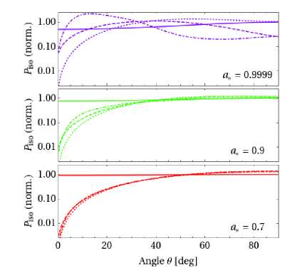
Figure 11: Isotropic power (eq. 55) for different spin parameters $a_{*}=\left\{0.7,0.9,0.9999\right\}$. The solid lines refer to the approximated analytic integration of eq. (56) plotted for intervals of $\left|\theta^{+}-\theta^{-}\right|=\pi/200$. The dashed lines show the direct integration of eq. (55) using the midpoint rule (i.e. using eq. 57). The dotted and dot-dashed lines represent the angular power derivation following the 4th, and 6th order approximations given by eqs.  (58) and (59), respectively. All lines are normalized to the maximum value of the isotropic power provided by eq. (56) in the interval $[0,\pi/2]$.

If the power of the BZ process drives a collimated relativistic outflow from the neighborhood of the BH, a distant observer may only see an small angular patch of the whole outflow due to relativistic beaming. Thus, following a common practice for the approximate estimation of the angular energy distribution in GRB ejecta (e.g. Janka et al., 2006; Mizuta & Aloy, 2009; Lazzati et al., 2009) that avoids performing a complete (and much more involved) radiation transport problem (Broderick & Blandford, 2003; Miller et al., 2003; Birkl et al., 2007; Cuesta-Martínez et al., 2015), it is useful to define an equivalent isotropic power $P_{\rm iso}{(\theta)}$ in each (narrow) angular region $\Delta\theta=\theta^{+}-\theta^{-}$ centered around $\theta$ (i.e. $\theta=(\theta^{+}-\theta^{-})/2$) as:

$$\begin{split}P_{\rm iso}\left(\theta\right)=&\>\frac{4\pi\epsilon_{0}}{\cos\theta^{-}-\cos\theta^{+}}\frac{a}{\Omega_{\rm\text{\tiny BH}}}\times\\ &\int_{\theta^{-}}^{\theta^{+}}\text{d}\theta\>\omega\left(\Omega_{\rm\text{\tiny BH}}-\omega\right)\frac{\sin\theta}{r_{+}^{2}+a^{2}\cos^{2}\theta}\>\left[\Psi_{,\theta}\right]^{2}\end{split}$$ (55)

This integral may be further simplified by using eq. (46) to replace $\left[\Psi_{,\theta}\right]^{2}$ by its angular average. The remaining integral is the same as in eq. (47) and can be solved analytically yielding,

$$\begin{split}P_{\rm iso}^{(1)}\left(\theta\right)=&\>\frac{2\pi\epsilon_{0}}{\cos\theta^{-}-\cos\theta^{+}}\frac{\Omega_{\rm\text{\tiny BH}}}{r_{+}^{2}+a^{2}}\left[\Psi_{,\theta}\right]^{2}\times\\ &\left\{\arctan{\left(\frac{a}{r_{+}}\cos\theta^{-}\right)}-\arctan{\left(\frac{a}{r_{+}}\cos\theta^{+}\right)}\right\}.\end{split}$$ (56)

Alternatively, eq. (55) can be computed using the midpoint approximation and plugging in for $\Psi_{,\theta}$ the angular derivative of $\Psi_{\rm f}\left(r_{+},\theta\right)$ as given in eq. (44). The angular dependence of the isotropic power then reduces to

$$P_{\rm iso}^{(2)}\left(\theta\right)={\frac{\pi\epsilon_{0}\Delta\theta}{\cos\theta^{+}-\cos\theta^{-}}}a\Omega_{\rm\text{\tiny BH}}\frac{\sin\theta}{r_{+}^{2}+a^{2}\cos^{2}\theta}\>\left[\Psi_{,\theta}\right]^{2}.$$ (57)

Figure 11 shows the isotropic power employing eq. (56) plotted for intervals of $\Delta\theta=\left|\theta^{+}-\theta^{-}\right|=\pi/200$, as well as the angular approximation given in eq. (57). For comparison, we also plot the isotropic equivalent power distribution following the 4th and 6th order approximations of Tchekhovskoy et al. (2010). Precisely, we show

$$P_{\rm iso,BZ4}(\theta)= \frac{2}{\cos\theta^{+}-\cos\theta^{-}}\left(P^{\rm cum}_{\rm BZ4}(\theta^{+})-P^{\rm cum}_{\rm BZ4}(\theta^{-})\right)\>,$$ (58)

and

$$P_{\rm iso,BZ6}(\theta)= \frac{2\Delta\theta}{\cos\theta^{+}-\cos\theta^{-}}\frac{dP_{\rm BZ6}}{d\theta}(\theta)\>,$$ (59)

where the 4th order accurate expression of the cumulative power as a function of the angle is (cf. Tchekhovskoy et al., 2010, eq. B6)

$$P^{\rm cum}_{\rm BZ4}(\theta)= \displaystyle\frac{1}{270}\pi\Omega_{\rm\text{\tiny BH}}^{4}\Bigg{(} 90\left(3\pi^{2}-32\right)\cos{(\theta)}+$$

$$5\left(194-21\pi^{2}\right)\cos{(3\theta)}+$$

$$9\left(3\pi^{2}-26\right)\cos(5\theta)+$$

$$32\left(67-6\pi^{2}\right)\Bigg{)}+$$

$$\displaystyle\frac{1}{3}\pi\Omega_{\rm\text{\tiny BH}}^{2}\Bigg{(} 4\sin^{4}\left(\frac{\theta}{2}\right)(\cos{(\theta)+2)}\Bigg{)}\>,$$

and the differential power per unit angle is given by

$$\frac{dP_{\rm BZ6}}{d\theta}(\theta)= \pi a\Omega_{\mbox{\rm\text{\tiny BH}}}\frac{\sin\theta}{r_{+}^{2}+a^{2}\cos^{2}\theta}\>\left[\Psi^{\rm(6)}_{,\theta}\right]^{2},$$

with $\Psi^{\rm(6)}_{,\theta}$ the angular derivative of the 6th order accurate approximation for the magnetic flux (cf. Tchekhovskoy et al., 2010, eqs. C1 and C2)

$$\Psi^{\rm(6)}= \>\Psi_{0}(r_{+},\theta)+16\Omega_{\mbox{\rm\text{\tiny BH}}}^{2}\frac{8(67-6\pi^{2})}{45}\sin^{2}\theta\cos\theta+$$

$$\>\Omega_{\mbox{\rm\text{\tiny BH}}}^{4}\sin^{2}\theta\>\left(26.12\cos^{25}\theta+22.72\cos^{7}\theta+\right.$$

$$\qquad\qquad\>\>\>\>\left.13.54\cos^{3}\theta+2.08\cos\theta\right).$$

Looking at the central and bottom panels of fig. 11, it is evident that estimating the isotropic equivalent power with the approximation leading to eq. (56) is not optimal, especially for $\theta\lesssim 40^{\circ}$ and moderate to large values of $a_{*}$. This is not surprising, since the average performed to compute (eq. 46) extends over the whole interval $\theta\in[0,\pi/2]$, while the isotropic power is evaluated for a relatively small angular patch, with angular extension $\Delta\theta$. Our isotropic power estimate employing the mid-point rule (eq. 57) yields much better results. It is closer to the 6th-order accurate estimation of eq. (59) than the 4th-order accurate estimation of eq. (58). However, it falls short to predict the isotropic power for $\theta\lesssim 25^{\circ}$ and almost maximal values of the BH spin ($a_{*}=0.9999$). At small or moderate values of $a_{*}\lesssim 0.7$, the isotropic power estimations yield quantitatively similar results, regardless of the approximation employed to compute the angular distribution of the BZ power (with the notable exception of $P_{\rm iso}^{(1)}(\theta)$). The differences show up more clearly as the value of $a_{*}$ grows. There is, however, a consistent trend in all cases: larger values of the BH spin parameter $a_{*}$ show larger powers closer to the axis of rotation. Indeed, we observe a transition in the curves of $P_{\rm iso}$. For $a_{*}>0.9$ the maximum value of $P_{\rm iso}$ shifts from $\theta=90^{\circ}$ to lower latitudes. For nearly maximally rotating BHs, the maximum isotropic equivalent power happens for $\theta\simeq 10^{\circ}$. Regardless of the exact location of the maximum, fig. 11 clearly shows that a distant observer would not see a maximum power for events seen “head-on”. Since the value of $P_{\rm iso}$ grows very steeply from zero, for events generated out of BHs with $a_{*}\gtrsim 0.9$, it is much more likely to observe luminous events when observing them at angles $\theta\gtrsim{10^{\circ}}$.

6 Discussion

Motivated by the study of relativistic outflows from spinning black holes (Blandford & Znajek, 1977), magnetospheric force-free electrodynamics for static and axisymmetric spacetimes have become a matter of active research (e.g. Camenzind, 2007; Beskin, 2010). Appl & Camenzind (1993) found the first non-linear analytical solution for a cylindrically collimated, asymptotic flux distribution, in special relativity. Until now, most of these studies have been done in the context of open field configurations, primarily because of its relevance to the jet problem. However, complex magnetic field topologies encompassing closed fieldlines may also develop in the course of the dynamical evolution arising from the accreting BHs (Goodman & Uzdensky, 2008; Parfrey et al., 2016). Indeed, it has been encountered in simulations of neutron star mergers (e.g. Rezzolla et al., 2011; Kiuchi et al., 2014), that the post merger BH magnetic fields are not necessarily of split-monopole or paraboloidal type. The exact topology of the magnetic field in the BH magnetosphere is of paramount importance to set the efficiency of energy extraction from the central compact object. This extraction of energy is supposed to be channeled out along the low-density funnel developed in the course of the merger around the rotational axis of the system. Especially in the low density funnel, field reversals have been encountered, possibly limiting the efficiency of outflow production.

Studying these phenomena requires accurate initial data for magnetospheric configurations and motivates us to build both transparent and versatile initial data solvers. In particular, it requires a proper characterization of the numerical methodology to solve the GSE.

The numerical method we propose splits into three basic blocks: (1) The finite difference solution of the GSE in each of the subdomains set by the light surfaces in the magnetosphere, (2) the matching of the solutions across the light surfaces to obtain regular functions, and (3) the build-up or update of the functional tables for $\omega(\Psi)$ and $II^{\prime}(\Psi)$.

We have shown that the convergence of the presented numerical technique greatly depends on a suitable selection of finite difference discretization around the LS and, hence, the diagonal dominance of the coefficient matrix of the SOR solver. Numerical artifacts develop around the LS if the ’smoothing-across-subdomains’ techniques are used (as in e.g. Nathanail & Contopoulos, 2014; Pan et al., 2017). These artifacts slow down the convergence of the GSE solution significantly, and the quality of the results is limited (see fig. 1). However, we find the choice of an inward/outward biased second order discretization around and with respect to the LS to be the most efficient setup to achieve fast convergence with convenient overrelaxation and no need for additional smoothing of the potential $\Psi$ across the LS.

We have extended the strategy of employing eq. (14) to relax the current $II^{\prime}\left(\Psi\right)$ (Uzdensky, 2004) also to the potential function $\omega$. This allows us to use the error of the GSE at the LS (eq. 11) as an additional measure of convergence for the presented numerical method. Despite the fact that we can also incorporate a local mesh refinement around the ILS, the method is, however, limited by the ability to fit sufficient grid cells between the BH horizon and the ILS. In the presented tests, we were able to ensure sufficient cells around the ILS for values as low as $a_{*}=0.5$. Nevertheless, the numerical solution of the GSE for spin factors lower than $a_{*}=0.7$ is perhaps unnecessary. As shown in fig. 5, even for a BH spin as large as $a_{*}=0.7$, the overall solution approached the initially guessed potential functions, which are the (exact) solutions of the case $a_{*}=0$. Thus, we find that with our method it is possible to explore the region very close to the horizon for rotating BHs with $a_{*}\gtrsim 0.7$. Resolving this region, which is near the location of the zero space-charge, and which is expected to be the source of the pairs that will populate the BH magnetosphere (Globus & Levinson, 2014), is very important for models of jet formation (as it is in pulsar magnetospheres; e.g. Belyaev & Parfrey, 2016).

In the literature, the solutions found by the numerical relaxation of the GSE seem to evolve towards a unique solution as long as the boundary conditions, especially the thin-disk assumption, hold (Contopoulos et al., 2013; Nathanail & Contopoulos, 2014). We have observed and discussed (see sec. 3.3) the relaxation of both potential functions $\omega$ and $I$ as a necessity for convergence under the criterion given in appendix (A.1). The relaxation of only one of these two functions may converge under the residual function $\mathcal{R}_{\Psi}$, but show non-convergence under the (mathematical) measure $\mathcal{R}_{LC}$, employing the GSE at the location of its singular surfaces (eq. 27). Hence, we cannot disprove the uniqueness of the solutions reproduced in sec. 4.

Proving the uniqueness of the solution of the GSE, given a set of boundary conditions, is not an easy task. The customary way of demonstrating uniqueness is to find a maximum principle. If no maximum principle can be found multiple solutions may arise for a given set of boundary conditions. Such an example can be found in Akgün et al. (2018), where the authors solved the Newtonian GSE equations without rotation for the case of a neutron star with a twisted magnetosphere, in some cases finding numerically multiple solutions with identical boundary conditions. In some particular cases uniqueness can be proven as in the case of current-free configurations (see e.g. Akgün et al., 2018) or for small twists (Bineau, 1972). Regarding black hole magnetospheres, Pan et al. (2017) have investigated the uniqueness of the solution of the GSE. These authors found that if the field lines cross smoothly the LSs (which is a ’constraint condition’ the solutions must satisfy), the boundary conditions at the horizon and at infinity are not independent. Therefore, for a given pair of functions $\omega(\Psi)$ and $I(\Psi)$ the boundary conditions are uniquely defined. Although this does not completely prove the uniqueness of the solution for given boundary conditions, it is a significant step in this direction. However, for the asymptotically uniform field, there is a variety of possibilities regarding uniqueness. Time-dependent simulations (e.g. Komissarov, 2005; Komissarov & McKinney, 2007; Yang et al., 2015) apparently converge to a unique solution. Several analytic studies find a unique perturbative solution that agrees with GRMHD simulations (Beskin & Zheltoukhov, 2013; Pan & Yu, 2015; Gralla et al., 2016).

As a byproduct of the study of split-monopole magnetospheres, we have provided an approximation for the potential $\Psi$ at the outer event horizon for different values of $a$ (eq. 44). In section 5, we examined the angular resolution as well as the total value of the power outflow (cf. Lee et al., 2000; Uzdensky, 2004) employing eq. (44). Especially for higher values of the BH spin parameter $a$ one finds a higher total power of the BZ process with more isotropic power provided closer to the axis of rotation and, hence, in the regions which are presumably critical for the production of BZ jets. Our estimations of the power of the BZ process using the fit formula (eq. 41) deviate less than 1% from the exact power computed numerically from the solutions of the GSE equations for the potential $\Psi$. Remarkably, this compares fairly well with the 4th order accurate expression of Tchekhovskoy et al. (2010) (their eq. B6), since their formula requires more than a factor of 3 correction to reproduce their numerical results for high BH spin (namely, $a_{*}\gtrsim 0.95$), as the authors point out. Thus, our relatively simple estimate of the BZ power provides estimates quantitatively comparable to the 6th order accurate expression of Tchekhovskoy et al. (2010; their eq. 9).

We also find that using our fit formula (eq. 44) to compute the angular derivative of the flux (which is proportional to the radial component of the magnetic field evaluated at the BH horizon; eq. 45) is an excellent approach to estimate the isotropic equivalent power as a function of the latitude. Our simple estimate is competitive with the 6th order accurate estimation of Tchekhovskoy et al. (2010) for BH spins $a_{*}\lesssim 0.98$. However, for nearly maximally rotating BH ($a_{*}\gtrsim 0.9999$), our isotropic equivalent power estimate falls short by factors $2-3$ with respect to the estimation employing a 6th order accurate formula. Remarkably, even for such large values of $a_{*}$, our mid-point approximation for the isotropic BZ luminosity (eq. 57) is better than the 4th order accurate estimation of eq. (58).

The stability of most of the stationary solutions found in this paper (and in the preceding literature in the field) has been assessed by means of time-dependent FFDE or GRMHD simulations (e.g. Komissarov, 2002, 2004; Tchekhovskoy et al., 2010) with a fixed background metric (the one provided by the BH). However, the stability of the solutions in cases where the space time may evolve due to the feedback between the BH and its magnetosphere has not been assessed so far. One application of the presented solving scheme will be the use of these configurations as initial data for time evolution simulations of dynamical spacetimes on the Carpet grid of the Einstein Toolkit. The discussed test cases are thought to be especially applicable in combination with recent methods to support rapidly rotating Kerr BHs in numerical simulations (Liu et al., 2009) and their numerically stable magnetohydrodynamic evolution (Faber et al., 2007). The current practice of evolving spacetimes without excising the BHs (for GRMHD simulations, cf. Faber et al., 2007) requires highly accurate initial data, especially at the BH apparent event horizons. The behavior under time evolution of dynamical spacetimes (without excising BHs) with the respective time-dependent feedback on the electromagnetic force-free fields will be an indicator on the stability of the found solutions of the GSE and may foster further optimization of the proposed numerical procedure. The results of the application of this methodology will be the subject of our subsequent work.

7 Acknowledgements

We thank the referee, Prof. I. Contopoulos, for his constructive comments and criticism. We kindly acknowledge Amir Levinson for his careful reading and feedback on the draft of this paper. We acknowledge the support from the European Research Council (grant CAMAP-259276) and the partial support of grants AYA2015-66899-C2-1-P and PROMETEO-II-2014-069. JM acknowledges the Grisolia Grant GRISOLIAP/2016/097 and a Ph.D. grant of the Studienstiftung des Deutschen Volkes. PC acknowledges the Ramon y Cajal program (RYC-2015-19074) supporting his research.

Appendix A Technical notes

A.1 Numerical convergence criteria

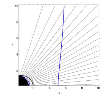
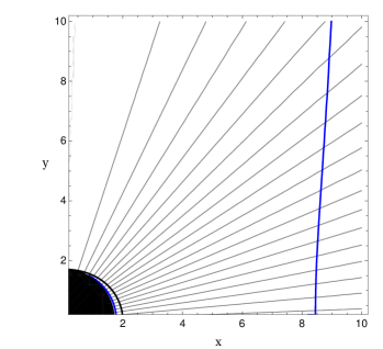
Figure 12: Distribution of the magnetic flux $\Psi$ in the vicinity of a black hole rotating at $a_{*}=0.999$ (top), $a_{*}=0.9$ (middle) and $a_{*}=0.7$ (bottom) after converging under the criteria in eq. (61) on the physical domain $[r_{+},\infty]\times[0,90^{\circ}]$, covered with a numerical grid $\left[n_{r}\times n_{\theta}\right]=\left[200\times 64\right]$. Both functions $\omega\left(\Psi\right)$ and $II^{\prime}\left(\Psi\right)$ are relaxed throughout the iterative procedure. The location of the ergosphere is represented by the black line, the two LS are drawn as blue lines.

As shown in figs. 1 and 2, the $L^{\infty}$ norm of the residual of the SOR scheme decreases rapidly for the applied biased stencil at the light surfaces. However, we find that a smooth solution for $\Psi$ in the entire domain (cf. sec. 2.1) requires an additional constraint imposed by the error $\mathcal{R}_{LC}$ at the LS. Kinks across a LS may remain present even though the solution converged under $\mathcal{R}_{\Psi}$. Furthermore, especially for non-extremal spin parameters $a$ we observe that both $\mathcal{R}_{LC}$ and $\mathcal{R}_{\Psi}$ are very small already in the first iterations of the solving routine. An exclusive focus on the residual $\mathcal{R}_{\Psi}$ may, hence, rapidly trigger a convergence decision without a full relaxation of $\omega$ and $II^{\prime}$. In these cases, kinks remain across the LS. For the shown tests we demand the simultaneous fulfillment of the following conditions as a convergence criterion:

$$\mathcal{R}_{\Psi}<10^{-6}\qquad\wedge\qquad\mathcal{R}_{LC}<5\times 10^{-4/\sqrt{a}}$$ (61)

Figure (12) shows selected split-monopole configurations after condition 61 has been reached. For different values of the black hole spin $a$, the required iterations to reach convergence are shown in table 2.

Spin ($a_{*}$)	Iterations until convergence
0.9999	50.161
0.999	29.100
0.99	64.117
0.9	43.153
0.8	12.100
0.7	19.129

Table 2: Number of iterations until the convergence criterion (61) is reached for the split-monopole setup described in section 4.1.

References

- Adsuara et al. (2016) Adsuara J. E., Cordero-Carrión I., Cerdá-Durán P., Aloy M. A., 2016, Journal of Computational Physics, 321, 369
- Akgün et al. (2018) Akgün T., Cerdá-Durán P., Miralles J. A., Pons J. A., 2018, MNRAS, 474, 625
- Appl & Camenzind (1993) Appl S., Camenzind M., 1993, A&A, 274, 699
- Belyaev & Parfrey (2016) Belyaev M. A., Parfrey K., 2016, ApJ, 830, 119
- Beskin (1997) Beskin V. S., 1997, Physics Uspekhi, 40, 659
- Beskin (2010) Beskin V. S., 2010, MHD Flows in Compact Astrophysical Objects. Springer, doi:10.1007/978-3-642-01290-7
- Beskin & Zheltoukhov (2013) Beskin V. S., Zheltoukhov A. A., 2013, Astronomy Letters, 39, 215
- Bineau (1972) Bineau M., 1972, Communications on Pure and Applied Mathematics, 25, 77
- Birkl et al. (2007) Birkl R., Aloy M. A., Janka H.-T., Müller E., 2007, A&A, 463, 51
- Blandford & Znajek (1977) Blandford R. D., Znajek R. L., 1977, MNRAS, 179, 433–456
- Broderick & Blandford (2003) Broderick A., Blandford R., 2003, MNRAS, 342, 1280
- Camenzind (1987) Camenzind M., 1987, A&A, 184, 341
- Camenzind (2007) Camenzind M., 2007, Compact Objects in Astrophysics: White Dwarfs, Neutron Stars, and Black Holes. Springer, doi:10.1007/978-3-540-49912-1
- Contopoulos et al. (1999) Contopoulos I., Kazanas D., Fendt C., 1999, ApJ, 511, 351–358
- Contopoulos et al. (2013) Contopoulos I., Kazanas D., Papadopoulos D. B., 2013, ApJ, 765, 113
- Cuesta-Martínez et al. (2015) Cuesta-Martínez C., Aloy M. A., Mimica P., 2015, MNRAS, 446, 1716
- Faber et al. (2007) Faber J. A., Baumgarte T. W., Etienne Z. B., Shapiro S. L., Taniguchi K., 2007, Phys. Rev. D, 76
- Fendt (1997) Fendt C., 1997, A&A, 319, 1025
- Garofalo (2009) Garofalo D., 2009, ApJ, 699, 400
- Ghosh (2000) Ghosh P., 2000, MNRAS, 315, 89–97
- Globus & Levinson (2014) Globus N., Levinson A., 2014, ApJ, 796, 26
- Goodman & Uzdensky (2008) Goodman J., Uzdensky D., 2008, ApJ, 688, 555
- Grad & Rubin (1958) Grad H., Rubin H., 1958, Proceedings of the Second United Nations Conference on the Peaceful Uses of Atomic Energy (Geneva), 31, 190
- Gralla et al. (2016) Gralla S. E., Lupsasca A., Rodriguez M. J., 2016, Phys. Rev. D, 93, 044038
- Hawley & Krolik (2006) Hawley J. F., Krolik J. H., 2006, ApJ, 641, 103
- Janka et al. (2006) Janka H.-T., Aloy M.-A., Mazzali P. A., Pian E., 2006, ApJ, 645, 1305
- Kiuchi et al. (2014) Kiuchi K., Kyutoku K., Sekiguchi Y., Shibata M., Wada T., 2014, Phys. Rev. D, 90
- Komissarov (2001) Komissarov S. S., 2001, MNRAS, 326, L41
- Komissarov (2002) Komissarov S. S., 2002, MNRAS, 336, 759–766
- Komissarov (2004) Komissarov S. S., 2004, MNRAS, 350, 427–448
- Komissarov (2005) Komissarov S. S., 2005, MNRAS, 359, 801
- Komissarov (2007) Komissarov S. S., 2007, MNRAS, 382, 995
- Komissarov (2009) Komissarov S. S., 2009, Journal of the Korean Physical Society, 54, 2503
- Komissarov & Barkov (2009) Komissarov S. S., Barkov M. V., 2009, MNRAS, 397, 1153–1168
- Komissarov & McKinney (2007) Komissarov S. S., McKinney J. C., 2007, MNRAS, 377, L49
- Lazzati et al. (2009) Lazzati D., Morsony B. J., Begelman M. C., 2009, ApJ, 700, L47
- Lee et al. (2000) Lee H. K., Wijers R., Brown G., 2000, Physics Reports, 325, 83–114
- Leveque & Li (1994) Leveque R. J., Li Z., 1994, SIAM Journal on Numerical Analysis, 31, 1019
- Liu et al. (2009) Liu Y. T., Etienne Z. B., Shapiro S. L., 2009, Phys. Rev. D, 80
- Lüst & Schlüter (1954) Lüst R., Schlüter A., 1954, Z. Astrophys., 34, 263
- MacDonald (1984) MacDonald D. A., 1984, MNRAS, 211, 313
- McKinney (2005) McKinney J. C., 2005, ApJ, 630, L5
- McKinney & Gammie (2004) McKinney J. C., Gammie C. F., 2004, ApJ, 611, 977–995
- Michel (1973) Michel F. C., 1973, ApJ, 180, L133
- Miller et al. (2003) Miller W. A., George N. D., Kheyfets A., McGhee J. M., 2003, ApJ, 583, 833
- Mizuta & Aloy (2009) Mizuta A., Aloy M. A., 2009, ApJ, 699, 1261
- Nagataki (2009) Nagataki S., 2009, ApJ, 704, 937
- Nathanail & Contopoulos (2014) Nathanail A., Contopoulos I., 2014, ApJ, 788, 186
- Nathanail et al. (2016) Nathanail A., Strantzalis A., Contopoulos I., 2016, MNRAS, 455, 4479
- Palenzuela et al. (2010) Palenzuela C., Garrett T., Lehner L., Liebling S. L., 2010, Phys. Rev. D, 82, 044045
- Palenzuela et al. (2011) Palenzuela C., Bona C., Lehner L., Reula O., 2011, Classical and Quantum Gravity, 28, 134007
- Pan & Yu (2015) Pan Z., Yu C., 2015, ApJ, 812, 57
- Pan & Yu (2016) Pan Z., Yu C., 2016, ApJ, 816, 77
- Pan et al. (2017) Pan Z., Yu C., Huang L., 2017, ApJ, 836, 193
- Parfrey et al. (2016) Parfrey K., Spitkovsky A., Beloborodov A. M., 2016, ApJ, 822, 33
- Penna et al. (2013) Penna R. F., Narayan R., Sa̧dowski A., 2013, MNRAS, 436, 3741
- Punsly (2001) Punsly B., 2001, Black Hole Gravitohydromagnetics. Springer, doi:10.1007/978-3-662-04409-4
- Reynolds et al. (2006) Reynolds C. S., Garofalo D., Begelman M. C., 2006, ApJ, 651, 1023
- Rezzolla et al. (2011) Rezzolla L., Giacomazzo B., Baiotti L., Granot J., Kouveliotou C., Aloy M. A., 2011, ApJ, 732, L6
- Ruderman & Sutherland (1975) Ruderman M. A., Sutherland P. G., 1975, ApJ, 196, 51
- Shafranov (1966) Shafranov V., 1966, Reviews of Plasma Physics, 2, 103
- Tanabe & Nagataki (2008) Tanabe K., Nagataki S., 2008, Phys. Rev. D, 78, 024004
- Tchekhovskoy & Giannios (2015) Tchekhovskoy A., Giannios D., 2015, MNRAS, 447, 327
- Tchekhovskoy et al. (2010) Tchekhovskoy A., Narayan R., McKinney J. C., 2010, ApJ, 711, 50
- Thorne et al. (1986) Thorne K. S., Price R. H., MacDonald D. A., eds, 1986, Black Holes: The Membrane Paradigm. Yale University Press
- Uzdensky (2004) Uzdensky D. A., 2004, ApJ, 603, 652–662
- Uzdensky (2005) Uzdensky D. A., 2005, ApJ, 620, 889
- Wald (1974) Wald R. M., 1974, Phys. Rev. D, 10, 1680
- Weber & Davis (1967) Weber E. J., Davis Leverett J., 1967, ApJ, 148, 217
- Yang et al. (2015) Yang H., Zhang F., Lehner L., 2015, Phys. Rev. D, 91, 124055
- Zhang (1989) Zhang X.-H., 1989, Phys. Rev. D, 39, 2933
- Znajek (1977) Znajek R. L., 1977, MNRAS, 179, 457–472