Quantum holography in a graphene flake with an irregular boundary

Abstract

Electrons in clean macroscopic samples of graphene exhibit an astonishing variety of quantum phases when strong perpendicular magnetic field is applied. These include integer and fractional quantum Hall states as well as symmetry broken phases and quantum Hall ferromagnetism. Here we show that mesoscopic graphene flakes in the regime of strong disorder and magnetic field can exhibit another remarkable quantum phase described by holographic duality to an extremal black hole in two dimensional anti-de Sitter space. This phase of matter can be characterized as a maximally chaotic non-Fermi liquid since it is described by a complex fermion version of the Sachdev-Ye-Kitaev model known to possess these remarkable properties.

Tensions between the laws of quantum mechanics and classical gravity that are emblematic of the extreme environments occurring in the early universe and near horizons of black holes constitute the most enigmatic mysteries in modern physics. A promising avenue to resolve some of the paradoxes encountered in these studies, such as the black hole information paradox, is the holographic principle Bousso (2002). In holographic duality, quantum gravity degrees of freedom in a $(d+1)$-dimensional spacetime “bulk” are represented by a many-body system defined on its $d$-dimensional boundary.

Important new insights into these fundamental questions have been gained recently through the study of the Sachdev-Ye-Kitaev (SYK) model Sachdev and Ye (1993); Kitaev (2015) which describes a system of $N$ fermions in (0+1) dimensions subject to random all-to-all four-fermion interactions and is dual to dilaton gravity in (1+1) dimensional anti-de Sitter space AdS₂ Sachdev (2015); Maldacena and Stanford (2016). Despite being maximally strongly interacting this model is, remarkably, exactly solvable in the limit of large $N$. It has been shown to exhibit physical properties characteristic of the black hole, including the extensive ground state entropy $S_{0}\sim N$, emergent conformal symmetry at low energy and fast scrambling of quantum information that saturates the fundamental bound on the relevant Lyapunov chaos exponent $\lambda_{T}$. Extensions of this model also show interesting behaviors, including unusual spectral properties You et al. (2017); Polchinski and Rosenhaus (2016); García-García and Verbaarschot (2016), supersymmetry Fu et al. (2017), quantum phase transitions of an unusual type Banerjee and Altman (2017); Bi et al. (2017); Lantagne-Hurtubise et al. (2018), quantum chaos propagation Gu et al. (2017); Berkooz et al. (2017); Hosur et al. (2016), patterns of entanglement Liu et al. (2018); Huang and Gu (2017) and strange metal behavior Song et al. (2017).

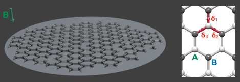
Figure 1: Schematic depiction of the proposed device. Irregular shaped graphene flake in applied magnetic field $B$ forms the (0+1) dimensional many-body system equivalent to a black hole in (1+1) anti-de Sitter space. Inset: lattice structure of graphene with A and B sublattices marked and nearest neighbor vectors denoted by ${\bm{\delta}}_{j}$.

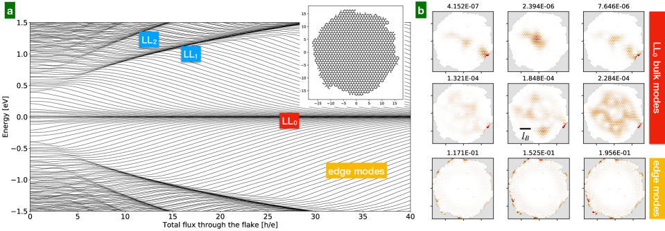
Figure 2: Electronic properties of an irregular graphene flake in the absence of interactions. a) Single-particle energy levels $\epsilon_{j}$ of the Hamiltonian $H_{0}$ as a function of the magnetic flux $\Phi=SB$ through the flake. The flake used for this calculation, depicted in the inset, consists of 1952 carbon atoms with equal number of A and B sites. The energy spectrum, calculated here in the Landau gauge ${\bm{A}}=Bx{\hat{\bm{y}}}$ and with open boundary conditions, shows the same generic features irrespective of the detailed flake geometry. b) Typical wavefunction amplitudes of the eigenstates $\Phi_{j}({\bm{r}})$ belonging to LL₀ at $\Phi=40\Phi_{0}$ and the edge modes. The numerals above each panel denote the energy $\epsilon_{j}$ of the state in eV, scale bar shows the magnetic length $l_{B}=\sqrt{\hbar c/eB}$.

In this letter we propose a simple experimental realization of the SYK model with complex fermions in a mesoscopic graphene flake with an irregular boundary and subject to a strong applied magnetic field. Unlike the earlier proposals in solid state systems Pikulin and Franz (2017); Chew et al. (2017), which targeted the Majorana fermion version of the model, our proposed device does not require superconductivity or advanced fabrication techniques and should therefore be relatively straightforward to assemble using only the existing technologies. The proposed design is illustrated in Fig. 1. Magnetic field $B$ applied to graphene is known to produce a variety of interesting quantum phases Novoselov et al. (2005); Zhang et al. (2005); Novoselov et al. (2007); Bolotin et al. (2009); Du et al. (2009); Dean et al. (2011); Feldman et al. (2012); Nomura and MacDonald (2006); Alicea and Fisher (2006); Amet et al. (2015). At the noninteracting level the field simply reorganizes the single-particle electron states into Dirac Landau levels with energies Castro Neto et al. (2009) $E_{n}\simeq\pm\hbar v\sqrt{2n(eB/\hbar c)}$ and $n=0,1,\cdots$. We argue that when the graphene flake is sufficiently small and irregular the electrons in the $n=0$ Landau level (LL₀) are generically described by the SYK model. This remarkable property is rooted in the celebrated Aharonov-Casher construction Aharonov and Casher (1979) which implies that, in the absence of interactions, LL₀ remains perfectly sharp even in the presence of strong disorder that respects the chiral symmetry of graphene. As we shall see a flake with a highly irregular boundary, illustrated in Fig. 1, is chirally symmetric. Electrons in LL₀, therefore, remain nearly perfectly degenerate, despite the fact that their wavefunctions acquire random spatial structure. When Coulomb repulsion is projected onto these highly disordered states, random all-to-all interactions between the zero modes are generated, exactly as required to define the SYK model.

The complex fermion SYK model, also known as the Sachdev-Ye (SY) model Sachdev and Ye (1993); French and Wong (1970); Bohigas and Flores (1971a, b), is defined by the second-quantized Hamiltonian

$${\cal H}_{\rm SY}=\sum_{ij;kl}J_{ij;kl}c^{\dagger}_{i}c^{\dagger}_{j}c_{k}c_{l}-\mu\sum_{j}c^{\dagger}_{j}c_{j},$$ (1)

where $c^{\dagger}_{j}$ creates a spinless fermion, $J_{ij;kl}$ are zero-mean complex random variables satisfying $J_{ij;kl}=J^{*}_{kl;ij}$ and $J_{ij;kl}=-J_{ji;kl}=-J_{ij;lk}$ and $\mu$ denotes the chemical potential. In what follows we derive the effective low-energy Hamiltonian for electrons in LL₀ of a graphene flake with an irregular boundary and show that, under a broad range of conditions, it is given by Eq. (1). The system, therefore, realizes the SY model.

At the non-interacting level a flake of graphene is described by a simple tight-binding Hamiltonian Castro Neto et al. (2009)

$$H_{0}=-t\sum_{{\bm{r}},{\bm{\delta}}}(a^{\dagger}_{\bm{r}}b_{{\bm{r}}+{\bm{\delta}}}+{\rm h.c.}),$$ (2)

where $a^{\dagger}_{\bm{r}}\ (b^{\dagger}_{{\bm{r}}+{\bm{\delta}}})$ denotes the creation operator of the electron on the subblatice A (B) of the honeycomb lattice. These satisfy the canonical anticommutation relations $\{a^{\dagger}_{\bm{r}},a_{{\bm{r}}^{\prime}}\}=\{b^{\dagger}_{\bm{r}},b_{{\bm{r}}^{\prime}}\}=\delta_{{\bm{r}}{\bm{r}}^{\prime}}$ appropriate for fermion operators. ${\bm{r}}$ extends over the sites in sublattice A while ${\bm{\delta}}$ denotes the 3 nearest neighbor vectors (inset Fig. 1). $t=2.7$ eV is the tunneling amplitude Song et al. (2010). For simplicity we first ignore electron spin but reintroduce it later. The chiral symmetry $\chi$ is generated by setting $(a_{\bm{r}},b_{\bm{r}}){\rightarrow}(-a_{\bm{r}},b_{\bm{r}})$ for all ${\bm{r}}$ which has the effect of flipping the sign of the Hamiltonian $H_{0}\to-H_{0}$.

Magnetic field $B$ is incorporated in the Hamiltonian (2) by means of the standard Peierls substitution which replaces $t\to t_{{\bm{r}},{\bm{r}}+{\bm{\delta}}}=t\exp{[-i(e/\hbar c)\int_{\bm{r}}^{{\bm{r}}+{\bm{\delta}}}{\bm{A}}\cdot{d\bm{l}}]}$ where ${\bm{A}}$ is the vector potential ${\bm{B}}=\nabla\times{\bm{A}}$. In the presence of $\chi$ the Aharonov-Casher construction Aharonov and Casher (1979) implies $N=N_{\Phi}$ exact zero modes in the spectrum of $H_{0}$ where $N_{\Phi}=SB/\Phi_{0}$ denotes the number of magnetic flux quanta $\Phi_{0}=hc/e$ piercing the area $S$ of the flake. It is clear that a flake with an arbitrary shape described by $H_{0}$ respects $\chi$ which underlies the robustness of LL₀ invoked above.

Hopping $t^{\prime}$ between second neighbor sites and random on-site potential are examples of perturbations that break $\chi$ and are therefore expected to broaden LL₀. These effects can be modeled by adding to ${\cal H}_{\rm SY}$ defined in Eq. (1) a term

$${\cal H}_{2}=\sum_{ij}K_{ij}c^{\dagger}_{i}c_{j}$$ (3)

which describes a small (undesirable) hybridization between the states in LL₀ that will generically be present in any realistic experimental realization. We discuss the effect of these terms below.

In Fig. 2a we show the single-particle energy spectrum of $H_{0}$ for a graphene flake with a shape depicted in the inset. As a function of increasing magnetic field $B$ we observe new levels joining the zero-energy manifold LL₀ such that the number of zero modes follows $N\simeq N_{\Phi}$ in accordance with the Aharonov-Casher argument. Higher Landau levels and topologically protected edge modes are also visible. Despite the randomness introduced by the irregular boundary LL₀ remains sharp as expected on the basis of the arguments presented above. This is the key feature in our construction of the SY Hamiltonian which guarantees that the ${\cal H}_{2}$ term defined above vanishes as long as the chiral symmetry is respected. In the presence of e-e repulsion the leading term in the effective description of LL₀ will therefore be a four-fermion interaction which we discuss next.

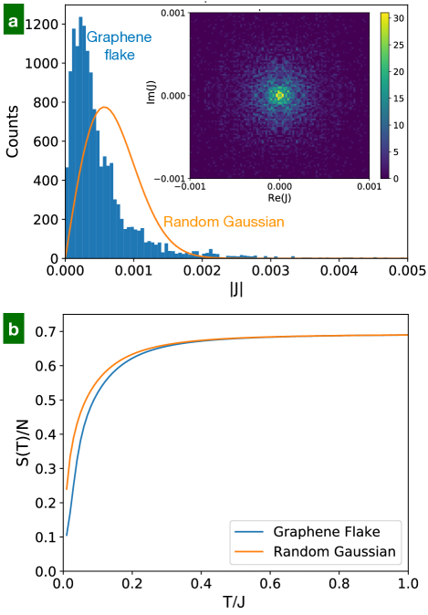
Figure 3: Statistical properties of the coupling constants and the thermal entropy. a) Histogram of $|J_{ij;kl}|$ as calculated from Eq. (4) with $V_{1}=1$ for the graphene flake depicted in Fig. 2 and $N=16$, compared to the Gaussian distribution (orange line) with the same variance $0.000805V_{1}$. Inset shows the histogram of real and imaginary components of $J_{ij;kl}$. The mirror symmetry about the horizontal follows from the hermiticity property $J_{ij;kl}=J^{*}_{kl;ij}$. b) Entropy $S(T)$ of the SY Hamiltonian (1) calculated with $J$s shown in panel (a).

Electron wavefunctions $\Phi_{j}({\bm{r}})$ belonging to LL₀ exhibit random spatial structure (Fig. 2b) owing to the irregular confining geometry imposed by the shape of the flake. From the knowledge of the wavefunctions it is straightforward to evaluate the corresponding interaction matrix elements (Supplementary Section A) between the zero modes. The leading many-body Hamiltonian for electrons in LL₀ will thus have the form of Eq. (1) with

$$J_{ij;kl}={1\over 2}\sum_{{\bm{r}}_{1},{\bm{r}}_{2}}[\Phi_{i}({\bm{r}}_{1})\Phi_{j}({\bm{r}}_{2})]^{*}V({\bm{r}}_{1}-{\bm{r}}_{2})[\Phi_{k}({\bm{r}}_{1})\Phi_{l}({\bm{r}}_{2})],$$ (4)

where $V({\bm{r}})=(e^{2}/\epsilon r)e^{-r/\lambda_{TF}}$ is the screened Coulomb potential with Thomas-Fermi length $\lambda_{TF}$ and dielectric constant $\epsilon$. The summation extends over all sites of the honeycomb lattice. It is to be noted that only the part of $J_{ij;kl}$ antisymmetric in $(i,j)$ and $(k,l)$ contributes to the many-body Hamiltonian (1) so in the following we assume that $J_{ij;kl}$ has been properly antisymmetrized.

We numerically evaluated $J_{ij;kl}$ for various values of $\lambda_{TF}$. The resulting $J$s are complex valued random variables satisfying

$$\overline{J_{ij;kl}}=0,\ \ \ \overline{|J_{ij;kl}|^{2}}={1\over 2N^{3}}J^{2},$$ (5)

where $J$ measures the interaction strength and the bar denotes averaging over randomness introduced by the irregular confining geometry. Fig. 3a shows the statistical distribution of $J_{ij;kl}$ calculated for the nearest-neighbor interactions $V({\bm{r}})=V_{1}\sum_{{\bm{\delta}}}\delta_{{\bm{r}},{\bm{\delta}}}$ and the single-particle wavefunctions $\Phi_{j}({\bm{r}})$ depicted in Fig. 2b. The distribution of $J_{ij;kl}$ shows the expected randomness with some deviations from the ideal Gaussian.

To ascertain the effect of these deviations and to prove that the low-energy fermions in the graphene flake are described by the SY model we next perform numerical diagonalization of the many-body Hamiltonian (1) with coupling constants $J_{ij;kl}$ obtained as described above. We then calculate various physical observables and compare them to the results obtained with random independent $J_{ij;kl}$. Fig. 3b shows the thermal entropy $S(T)$ of the flake. Comparison to the entropy calculated with random Gaussian $J_{ij;kl}$ indicates no significant difference. It is to be noted that while the SY model is known to exhibit non-zero ground state entropy per particle in the thermodynamic limit, $S(T)$ still vanishes as $T\to 0$ for any finite $N$ Fu and Sachdev (2016).

$N(\!\!\mod{4})$	0	1	2	3
$q=0$	GOE		GSE
$q\neq 0$	GUE	GUE	GUE	GUE

Table 1: Gaussian ensembles for the SY model. The relevant probability distributions are given by Eq. (6) with $Z={8\over 27},{4\pi\over 81\sqrt{3}},{4\pi\over 729\sqrt{3}}$ and $\beta=1,2,4$ for GOE, GUE, GSE, respectively.

Many-body energy level statistics provide another useful tool to validate our hypothesis that LL₀ electrons in the graphene flake behave according to the SY model. We thus arrange the energy eigenvalues $E_{n}$ of the many-body Hamiltonian (1) in increasing order and form ratios of the subsequent levels $r_{n}=(E_{n+1}-E_{n})/(E_{n}-E_{n-1})$. According to the random matrix theory applied to the SY model You et al. (2017) probability distributions $P(\{r_{n}\})$ are given by different Gaussian ensembles, depending on $N(\!\!\mod 4)$ and the eigenvalue $q$ of the total charge operator $Q=\sum_{j}(c^{\dagger}_{j}c_{j}-1/2)$ as summarized in Table I. Here GOE, GUE and GSE stand for Gaussian orthogonal, unitary and symplectic ensembles, respectively and

$$P(r)={1\over Z}{(r+r^{2})^{\beta}\over(1+r+r^{2})^{1+3\beta/2}},$$ (6)

with constants $Z$ and $\beta$ listed in Table I. Since ${\cal H}_{\rm SY}$ commutes with $Q$ it can be block diagonalized in sectors with definite charge eigenvalue $q$. As emphasized in Ref. You et al., 2017 the level statistics analysis must be performed separately for each $q$-sector. Note that $q$ has integer (half-integer) values for $N$ even (odd) and this is why the neutrality condition $q=0$ can be met only for even values of $N$. Also note that $q=0$ corresponds to $N/2$ particles.

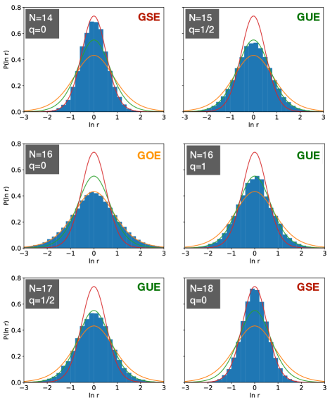
Figure 4: Many-body level statistics for the interacting electrons in LL₀ of the graphene flake. Blue bars show the calculated distributions for the graphene flake. Orange, green and red curves indicate the expected distributions given by Eq. (6) for GOE, GUE and GSE, respectively. To obtain smooth distributions, results for $N=14,15,(16)$ have been averaged over 8 (4) distinct flake geometry realizations while $N=17,18$ reflect a single realization.

Fig. 4 shows our results for the level statistics performed for a graphene flake with $N=14$ through $18$ and various values of $q$. The obtained level spacing distributions are seen to unambiguously follow the prediction of the random matrix theory for the SY model summarized in Table I. We are thus led to conclude that interacting electrons in LL₀ of a graphene flake with an irregular boundary indeed exhibit spectral properties characteristic of the SY model.

In the rest of this Letter we discuss various aspects of the problem relevant to the laboratory realization. Electrons in graphene possess spin which we so far ignored. Given the weak spin-orbit coupling in graphene we may model the non-interacting system by two copies of the Hamiltonian Eq. (2) plus the Zeeman term, $H=H_{0}+g^{*}\mu_{B}{\bm{B}}\cdot{\bm{S}}_{\rm tot}$ where ${\bm{S}}_{\rm tot}$ is the total spin operator and $\mu_{B}=5.78\times 10^{-5}$ eV/T is the Bohr magneton. For graphene on the SiO₂ or hBN substrate we may take $g^{*}\simeq 2$ which gives the bare Zeeman splitting $\Delta E_{S}(B)\simeq 0.12$ meV/T, or about 2.4 meV at $B=20$ T. We expect this relatively small spin splitting to be significantly enhanced by the exchange effect of the Coulomb repulsion. The strength of the exchange splitting $\Delta E_{C}\simeq 8.8$ meV/T is estimated in the Supplementary Section A. For such a large spin splitting one may focus on a partially filled LL₀ for a single spin projection and disregard the other. The spinless model considered so far should therefore serve as an excellent approximation of the physical system in the strong field.

Disorder that breaks chiral symmetry will inevitably be present in real graphene samples. Such disorder tends to broaden LL₀ and compete with the interaction effects that underlie the SY physics. It is known that bilinear terms ${\cal H}_{2}$ that arise from such disorder constitute a relevant perturbation to ${\cal H}_{\rm SY}$ and drive the system towards a disordered Fermi liquid (dFL) ground state. In the Supplementary Section B we analyze the symmetry-breaking effects and estimate their strength in realistic situations. We conclude that in carefully prepared samples a significant window should remain open at non-zero temperatures and frequencies in which the system exhibits behavior characteristic of the SY model.

An ideal sample to observe the SY physics is a graphene flake with a highly irregular boundary and clean interior. These conditions promote random spatial structure of the electron wavefunctions and preserve degeneracy of LL₀. Disordered wavefunctions give rise to random interaction matrix elements $J_{ij;kl}$ while near-degeneracy of states in LL₀ guarantees that the two-fermion term ${\cal H}_{2}$ remains small. To observe signatures of the emergent black hole the LL₀ degeneracy $N=SB/\Phi_{0}$ must be reasonably large – numerical simulations indicate that $N\gtrsim 10$ is required for the system to start showing the characteristic spectral features. Aiming at $N\simeq 100$, which is well beyond what one can conceivably simulate on a computer, implies the characteristic sample size $L\simeq\sqrt{S}=\sqrt{N\Phi_{0}/B}\simeq 150$ nm at $B=20$ T. Signatures of the SY physics can be observed spectroscopically, e.g. by the differential tunneling conductance $g(V)=dI/dV$ which is predicted Pikulin and Franz (2017) to exhibit a characteristic square-root divergence $g(V)\sim|V|^{-1/2}$ in the SY regime at large $N$, easily distinguishable from the dFL behavior $g(V)\sim$ const at small $V$. We predict that a tunneling experiment will observe the SY behavior when the chemical potential of the flake is tuned to lie in LL₀ and dFL behavior for all LL_n with $n\neq 0$. We also expect the two-terminal conductance across the flake to show interesting behavior in the SY regime but we defer a detailed discussion of this to future work.

In the limit of a large flake the irregular boundary will eventually become unimportant for the electrons in the bulk interior and the system should undergo a crossover to a more conventional ‘clean’ phenomenology characteristic of graphene in applied magnetic field. The exact nature of this crossover poses an interesting theoretical as well as experimental problem which we also leave to future study.

Acknowledgments – The authors are indebted to Ian Affleck, Oguzhan Can, Étienne Lantagne-Hurtubise and Chengshu Li for stimulating discussions. The work was supported by NSERC, CIfAR (AC,MF) and by the Marie Curie Programme under EC Grant agreement No. 705968 (FJ)”. Tight-binding simulations were performed using Kwant code  Groth et al. (2014) and computational resources provided by WestGrid.

I Supplementary material

I.1 Exchange splitting and the interaction matrix elements

In this section we discuss the enhancement of the Zeeman splitting due to the exchange interaction, derive the form of coupling constants $J_{ij;kl}$ quoted in Eq. (4) of the main text and estimate the characteristic interaction strength $J$.

I.1.1 General considerations

We begin by writing the Hamiltonian for the electrons in graphene as $H=H_{0}+H_{\rm int}$ where

$$H_{0}=-\sum_{\langle{\bm{r}},{\bm{r}}^{\prime}\rangle,\sigma}t_{{\bm{r}}{\bm{r}}^{\prime}}f_{{\bm{r}}\sigma}^{\dagger}f_{{\bm{r}}^{\prime}\sigma}+{g^{*}\mu_{B}B\over 2}\sum_{{\bm{r}}}(\rho_{{\bm{r}}\uparrow}-\rho_{{\bm{r}}\downarrow}),$$ (S1)

Here $f_{{\bm{r}}\sigma}^{\dagger}$ creates an electron with spin $\sigma$ on the site ${\bm{r}}$ of the honeycomb lattice and satisfies $\{f_{{\bm{r}}\sigma}^{\dagger},f_{{\bm{r}}^{\prime}\sigma^{\prime}}\}=\delta_{{\bm{r}}{\bm{r}}^{\prime}}\delta_{\sigma\sigma^{\prime}}$. Relative to our notation in Eq. (2) of the main text we added the spin degree of freedom. Aside from the spin degree of freedom $f_{{\bm{r}}\sigma}$ coincides with $a_{\bm{r}}$ ($b_{\bm{r}}$) when ${\bm{r}}$ is in subblattice A (B). Peierls substitution implies $t_{{\bm{r}}{\bm{r}}^{\prime}}=t\exp{[-i(e/\hbar c)\int_{\bm{r}}^{{\bm{r}}^{\prime}}{\bm{A}}\cdot{d\bm{l}}]}$ for the hopping integral in the presence of the magnetic field ${\bm{B}}=\nabla\times{\bm{A}}$ and $\rho_{{\bm{r}}\sigma}=f_{{\bm{r}}\sigma}^{\dagger}f_{{\bm{r}}\sigma}$ is the electron number on site ${\bm{r}}$ with spin $\sigma$.

To specify the flake shape, we start with a circle divided into a number $P$ of wedges, each of which has radius randomly chosen between $R_{-}$ and $R_{+}$. This procedure generates a compact shape with an irregular boundary. The graphene tight-binding model is then implemented on the resulting shape using the Kwant Python package Groth et al. (2014).

Interactions are described by

$$H_{\rm int}={1\over 2}\sum_{{\bm{r}},{\bm{r}}^{\prime}}\rho_{\bm{r}}V({\bm{r}}-{\bm{r}}^{\prime})\rho_{{\bm{r}}^{\prime}},$$ (S2)

where $\rho_{\bm{r}}=\rho_{{\bm{r}}\uparrow}+\rho_{{\bm{r}}\downarrow}$ represents the total charge on site ${\bm{r}}$ and $V({\bm{r}})=(e^{2}/\epsilon r)e^{-r/\lambda_{TF}}$ is the screened Coulomb potential.

Our strategy is to first solve the non-interacting problem defined by $H_{0}$ on a flake with an irregular boundary. This yields a set of single-particle energy levels $\epsilon_{j}$ and the corresponding eigenstates $\Phi_{j}({\bm{r}})$. As already discussed in the main text the energy levels consist of bulk Landau levels and edge modes. The Zeeman term simply offsets the spin-up bands by $\Delta E_{S}(B)=g^{*}\mu_{B}B$ with respect to spin-down bands.

Next we write the interaction term $H_{\rm int}$ in the basis defined by the eigenstates $\Phi_{j}({\bm{r}})$. If $c_{j\sigma}^{\dagger}$ creates a particle with spin $\sigma$ in eigenstate $\Phi_{j}({\bm{r}})$ we have $\rho_{\bm{r}}=\sum_{i,j,\sigma}\Phi_{i}^{*}({\bm{r}})\Phi_{j}({\bm{r}})c_{i\sigma}^{\dagger}c_{j\sigma}$. Substituting into Eq. (S2) and rearranging we find

$$H_{\rm int}=\sum_{i,j,k,l}\sum_{\sigma,\sigma^{\prime}}J_{ij;kl}c_{i\sigma}^{\dagger}c_{j\sigma^{\prime}}^{\dagger}c_{k\sigma^{\prime}}c_{l\sigma},$$ (S3)

where $J_{ij;kl}$ is given by Eq. (3) in the main text.

Henceforth we focus on the states belonging to LL₀, that is, we consider electron densities such that all Landau levels with negative energies are filled, while LL₀ is partially filled. Given the LL degeneracy $N=SB/\Phi_{0}$ per spin we define the total number of LL₀ electrons $N_{F}$ such that $N_{F}=0$ and $N_{F}=2N$ correspond to completely empty or filled LL₀, respectively. Because higher LLs are separated by an energy gap, for sufficiently weak interactions we can disregard virtual transitions into these bands and project $H_{\rm int}$ onto LL₀ by simply restricting all indices $(i,j,k,l)$ in Eq. (S3) to those labeling eigenstates $\Phi_{j}$ in LL₀.

I.1.2 Exchange splitting

We expect electrons to occupy LL₀ in such a way as to maximize the total spin ${\bm{S}}_{\rm tot}$ with $S^{z}_{\rm tot}$ aligned with the field. Such a state will minimize the Zeeman energy as well as the Coulomb repulsion due to the exchange effect. The latter arises because when the spin part of the many-body electron wavefunction is symmetric in spin degrees of freedom the spatial part must necessarily be antisymmetric. This forces $\Psi({\bm{r}}_{1},{\bm{r}}_{2},\dots)$ to vanish whenever two electron positions coincide, which tends to minimize the short-range part of the Coulomb repulsion energy. While the Zeeman splitting is easy to determine (main text), estimation of the exchange splitting magnitude for $N_{F}$ fermions described by Eq. (S3) is a non-trivial task. This is because couplings $J_{ij;kl}$ are all-to-all and essentially random. To get an idea about the expected magnitude of the exchange splitting we consider below a simple case of $N=N_{F}=2$.

For two electrons the position space wavefunction can be either symmetric or antisymmetric under exchange depending on the spin state, $\Psi_{\pm}({\bm{r}}_{1},{\bm{r}}_{2})={1\over\sqrt{2}}\left[\Phi_{1}({\bm{r}}_{1})\Phi_{2}({\bm{r}}_{2})\pm\Phi_{1}({\bm{r}}_{2})\Phi_{2}({\bm{r}}_{1})\right]$. The corresponding Coulomb energy is $E_{C}^{\pm}=\sum_{{\bm{r}}_{1},{\bm{r}}_{2}}|\Psi_{\pm}({\bm{r}}_{1},{\bm{r}}_{2})|^{2}V({\bm{r}}_{1}-{\bm{r}}_{2})$. The exchange splitting, then, becomes simply $\Delta E_{C}=E_{C}^{+}-E_{C}^{-}$ and reads

$$\Delta E_{C}=2\sum_{{\bm{r}}_{1},{\bm{r}}_{2}}{\rm Re}\left[\Phi_{1}^{*}({\bm{r}}_{1})\Phi_{2}({\bm{r}}_{1})V({\bm{r}}_{1}-{\bm{r}}_{2})\Phi_{2}^{*}({\bm{r}}_{2})\Phi_{1}({\bm{r}}_{2})\right]$$ (S4)

In order to estimate $\Delta E_{C}$ from Eq. (S4) we make an assumption, motivated by our extensive numerical work, that on lengthscales larger than the magnetic length $l_{B}=\sqrt{\hbar c/eB}$ wavefunctions $\Phi_{j}({\bm{r}})$ behave as random uncorrelated variables. We thus coarse grain the wavefunctions on a grid with sites denoted by ${\bm{R}}$ and spacing $l_{B}$. The coarse-grained wavefunctions $\Phi_{j}({\bm{R}})$ are then treated as complex-valued independent random variables with

$$\overline{\Phi_{j}({\bm{R}})}=0,\ \ \ \ \overline{\Phi_{i}^{*}({\bm{R}})\Phi_{j}({\bm{R}}^{\prime})}={1\over M_{s}}\delta_{ij}\delta_{{\bm{R}}{\bm{R}}^{\prime}}.$$ (S5)

Overbar denotes averaging over independent realizations of the flake geometry. The second equality in Eq. (S5) follows from the normalization of $\Phi_{j}$ and

$$M_{s}=S/l_{B}^{2}=2\pi N$$ (S6)

denotes the number of grid sites in the flake.

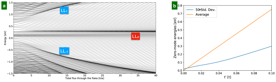
Figure S1: Effects of the second neighbor hopping $t^{\prime}$. a) Single-particle energy spectrum of a flake (the same geometry as Fig. 2 main text) with second neighbor hopping $t^{\prime}=0.037t$. b) Average shift $\delta{\epsilon}=\overline{K_{ij}}$ and standard deviation $K$ of 40 energy levels that comprise LL₀ as a function of $t^{\prime}$.

With this preparation we now recast Eq.  (S4) as a sum over the coarse grained grid, $\sum_{{\bm{r}}_{1},{\bm{r}}_{2}}\to\sum_{{\bm{R}}_{1},{\bm{R}}_{2}}$ and $\Phi_{j}({\bm{r}})\to\Phi_{j}({\bm{R}})$. Using Eq. (S5) we then obtain an estimate for the typical exchange splitting

$$\Delta E_{C}\simeq{2\over M_{s}^{2}}\sum_{{\bm{R}}_{1},{\bm{R}}_{2}}\delta_{{\bm{R}}_{1}{\bm{R}}_{2}}V({\bm{R}}_{1}-{\bm{R}}_{2})={2\over M_{s}}V(0).$$ (S7)

Here $V(0)$ must be interpreted as the average Coulomb potential in a grid patch of the size $l_{B}$, that is $V(0)\simeq(1/\pi l_{B}^{2})\int_{0}^{l_{B}}V(r)2\pi rdr=2e^{2}/\epsilon l_{B}$, where we assumed $\lambda_{TF}\gg l_{B}$. Taking the dielectric constant $\epsilon=2$ and $N=2$ we find the typical exchange splitting $\Delta E_{C}\simeq 8.8$ meV/T. We expect this result to remain at least approximately valid for $N>2$. Therefore, when $N_{F}<N$, electrons will fill the spin-down states of LL₀ with empty spin-up states separated in energy by a significant exchange gap. The physics of such partially filled spin-down LL₀ can be described by the Hamiltonian (S3) with $\sigma=\sigma^{\prime}=\downarrow$ which is precisely the SY Hamiltonian.

I.1.3 Coupling strength $J$

To estimate the typical strength of couplings $J_{ij;kl}$ that enter the SY Hamiltonian it is useful to first recast Eq. (4) of the main text such that it is explicitly antisymmetric in indices $(i,j)$ and $(k,l)$

$$J_{ij;kl}={1\over 2}\sum_{{\bm{R}}_{1},{\bm{R}}_{2}}\Omega_{ij}^{*}({\bm{R}}_{1},{\bm{R}}_{2})V({\bm{R}}_{1}-{\bm{R}}_{2})\Omega_{kl}({\bm{R}}_{1},{\bm{R}}_{2}),$$ (S8)

where $\Omega_{ij}({\bm{R}}_{1},{\bm{R}}_{2})={1\over 2}[\Phi_{i}({\bm{R}}_{1}),\Phi_{j}({\bm{R}}_{2})]$. We also passed to the coarse-grained variables, as described above. With help of Eq. (S5) it is straightforward to show that $\overline{J_{ij;kl}}=0$ and

$$\overline{|J_{ij;kl}|^{2}}={1\over M_{s}^{3}}\sum_{{\bm{R}}\neq 0}V({\bm{R}})^{2}.$$ (S9)

The sum can be approximated by an integral,

$$\int_{l_{B}\over 2}^{\infty}{2\pi RdR\over l_{B}^{2}}\left({e^{2}\over\epsilon}{e^{-R/\lambda_{TF}}\over R}\right)^{2}=\left({e^{2}\over\epsilon l_{B}}\right)^{2}2\pi\Gamma(0,{l_{B}\over\lambda_{TF}}),$$ (S10)

where $\Gamma(0,x)=\int_{x}^{\infty}dy\ e^{-y}/y$ is the incomplete gamma function. Combining with Eq. (5) in the main text we thus obtain an estimate

$$J\simeq 2\left({e^{2}\over\epsilon l_{B}}\right)\left(N\over M_{s}\right)^{3/2}\sqrt{\pi\Gamma(0,{l_{B}\over\lambda_{TF}})}.$$ (S11)

For $\epsilon=2$ this amounts to

$$J\simeq 6.04\ {\rm meV}\sqrt{B[{\rm T}]\ \Gamma(0,{l_{B}\over\lambda_{TF}})}.$$ (S12)

For $x=l_{B}/\lambda_{TF}\ll 1$, which is the limit of interest, $\Gamma(0,x)\simeq\ln(1/x)$ so $J$ is only very weakly dependent on the screening length. For $B=20$ T and $\lambda_{TF}/l_{B}=4$ we obtain $J\simeq 25$ meV.

It is to be noted that our numerical calculations of $J_{ij;kl}$ described in the main text [discussion below Eq. (5)] give larger values of $J$ than the above estimate, in some cases by as much as an order of magnitude. The discrepancy is most likely attributable to the fact that LL₀ wavefunctions are in fact disordered on a somewhat longer lengthscale than $l_{B}$. This would modify the relation between $M_{s}$ and $N$ given by Eq. (S6) and increase the ratio $(N/M_{s})$ that enters the estimate for $J$ in Eq. (S11). We may therefore regard Eq. (S11) as a conservative lower bound on the expected magnitude of $J$. This is already a large energy scale which should make the manifestations of the SY physics experimentally observable at low temperatures in clean graphene flakes.

I.2 Symmetry breaking perturbations

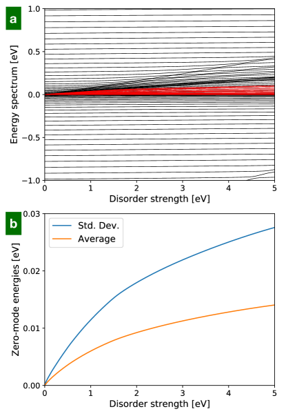
Figure S2: Effects of random on-site potential. a) Low-energy part of the numerically calculated energy spectrum for the flake with $n_{I}=1$% of defected sites as a function of the disorder potential strength $w$ and $N=40$. b) Average shift $\delta{\epsilon}=\overline{K_{ij}}$ and standard deviation $K$ of 40 energy levels that evolve from the zero modes which comprise LL₀ in the pure sample. These levels are marked in red in panel (a).

To ascertain the experimental feasibility of our proposal we now discuss the effect of various chiral symmetry breaking perturbations that exist in real graphene. Such perturbations tend to broaden LL₀ and can be modeled by a bilinear term ${\cal H}_{2}$ defined by Eq. (3) in the main text. The matrix elements are

$$K_{ij}=\sum_{\bm{r}}\Phi_{i}^{*}({\bm{r}})H^{\prime}({\bm{r}})\Phi_{j}({\bm{r}}),$$ (S13)

where $H^{\prime}$ denotes the Hamiltonian of the perturbation. The strength of these perturbations is measured by parameter $K$ defined as

$$K^{2}=N\left(\overline{|K_{ij}|^{2}}-|\overline{K_{ij}}|^{2}\right).$$ (S14)

It is known that since ${\cal H}_{2}$ is a relevant perturbation to ${\cal H}_{\rm SY}$ (in the renormalization group sense) the ground state of the system becomes a (disordered) Fermi liquid for any nonzero $K$. Nevertheless, if $K\ll J$, a significant crossover region can exist at finite frequencies and temperatures in which the system behaves effectively as a maximally chaotic SY liquid. According to the analysis of Ref. Pikulin and Franz, 2017 the zero-temperature propagator of the system with both $K$ and $J$ nonzero exhibits the SY conformal scaling $G(\omega)\sim|\omega|^{-1/2}$ for frequencies satisfying

$$16\sqrt{\pi}K^{2}/J<\omega\ll J.$$ (S15)

In the following we consider two specific perturbations that are present in real graphene, the second neighbor hopping $t^{\prime}$ and random on-site potential. Both break the chiral symmetry $\chi$ and produce non-zero parameter $K$. We derive limits on the admissible strength of these perturbations based on the requirement that Eq. (S15) yields a significant window in which SY behavior can be observed.

I.2.1 Second neighbor hopping

We first consider second neighbor hopping with the Hamiltonian acting as $H^{\prime}({\bm{r}})\Phi_{j}({\bm{r}})=t^{\prime}\sum_{{\bm{a}}}\Phi_{j}({\bm{r}}+{\bm{a}})$. Here ${\bm{a}}$ denotes the 3 second neighbor vectors in the honeycomb lattice. Since $|{\bm{a}}|\ll l_{B}$ we find, upon coarse graining the sum in Eq. (S13),

$$K_{ij}\simeq 3t^{\prime}\sum_{\bm{R}}\Phi_{i}^{*}({\bm{R}})\Phi_{j}({\bm{R}}).$$ (S16)

With help of Eq. (S5) it is straightforward to show that

$$\overline{K_{ij}}\simeq 3t^{\prime}\delta_{ij},\ \ \ \ \overline{|K_{ij}|^{2}}\simeq 9t^{\prime 2}\left(\delta_{ij}+M_{s}^{-1}\right).$$ (S17)

From Eq. (S14) we get $K\simeq 3t^{\prime}\sqrt{N/M_{s}}\simeq 3t^{\prime}/\sqrt{2\pi}$ independent of the field.

Experimentally reported values of $t^{\prime}$ range betweenCastro Neto et al. (2009) 1-3% of $t$ which would produce a rather large broadening of LL₀ in real graphene, $K\simeq 30-90$ meV. On the other hand existing experiments Song et al. (2010) indicate much smaller broadening of Landau levels in graphene of at most several meV which also includes broadening due to impurities and other defects. We therefore conclude that the above method must severely overestimate the contribution of second neighbor hopping to parameter $K$. This conclusion is supported by our numerical results presented below.

The numerically computed energy spectrum of the graphene flake with second neighbor hopping $t^{\prime}=0.037t$ is displayed in Fig. S1a. We observe that while LL₀ is now significantly shifted away from zero energy it remains sharp and well defined. The overall upward shift of LL₀ by about 0.25 eV is consistent with the estimate given in Eq. (S17) which implies $\overline{K_{ij}}\simeq 0.30$ eV. The broadening induced by $t^{\prime}$ is quantified in Fig. S1b and is well approximated by a linear dependence $K\simeq 0.022t^{\prime}$. This is about a factor of 50 smaller than the estimate implied by Eq. (S17). For $t^{\prime}=0.02t$ we obtain $K\simeq 1.2$ meV, a result that is much more in line with the experimental data.

The discrepancy between the analytical estimate and the numerical result can be understood as follows. In a large, disorder-free sample of graphene, inclusion of the second neighbor hopping produces changes in the band structure (and thus the position and spacing of LLs) but does not give rise to any LL broadening as long as $t^{\prime}$ remains spatially uniform. The sharpness of LLs is protected by translational invariance, not the chiral symmetry. In our mesoscopic flake we see that the inclusion of a spatially uniform $t^{\prime}$ primarily shifts the position of LLs, as expected from the argument given above. Because randomness is present in the system due to its irregular geometry some broadening occurs. This broadening is, however, much weaker than what is predicted by the naive estimate.

I.2.2 Random on-site potential

Random on-site potential is implemented by taking $H^{\prime}({\bm{r}})=w\sum_{{\bm{r}}^{\prime}\in{\cal I}}\delta_{{\bm{r}}{\bm{r}}^{\prime}}$, where $\cal I$ denotes a set of randomly chosen sites with number density $n_{I}$ in the graphene lattice and $w$ controls the disorder potential strength. Substituting $H^{\prime}$ into Eq. (S13) leads to the same result as indicated in Eq. (S17) with $3t^{\prime}$ replaced by $wn_{I}$. We therefore expect an overall energy shift of LL₀ by $wn_{I}$ accompanied by a broadening

$$K\simeq wn_{I}\sqrt{N\over M_{s}}.$$ (S18)

Fig. S2a shows the numerically computed energy eigenvalues as a function of $w$ for a flake with $N=40$ flux quanta and $n_{I}=1$%. We observe that LL₀ is shifted upward as well as broadened with increasing disorder strength. This shift $\delta\epsilon$ and broadening $K$ are quantified in Fig. S2b. At small $w$ these satisfy $\delta\epsilon\simeq 0.8n_{I}w$ and $K\simeq 1.3n_{I}w$ while at larger values the dependence is no longer linear, presumably because the system enters a non-perturbative regime when $w$ becomes comparable to the bandwidth. We see that the numerically obtained shift in LL₀ is well aligned with the analytical estimate. The broadening $K$ also agrees if we take $\sqrt{N/M_{s}}\simeq 1.3$ (instead of $1/\sqrt{2\pi}\simeq 0.4$ implied by Eq.  S6). This result reinforces the conclusion, reached in Appendix A by comparing the interaction strength estimate to the numerical calculation, that the zero mode wavefunction disorder scale is somewhat longer than $l_{B}$.

We finally remark that in the above example 40 flux quanta through a flake with 1952 carbon atoms correspond to an unrealistically high magnetic field of $\sim 3200$ T. Such high fields are needed for us to be able to numerically simulate meaningful number of zero modes $N$ with available computational resources. To make a closer contact with experiment we may however reinterpret these results by viewing the honeycomb lattice not as the atomic carbon lattice but as a convenient regularization of the low energy theory of Dirac electrons in graphene. In such low energy theory the only important parameter is the Dirac velocity $v_{F}={3\over 2}ta\simeq 1.1\times 10^{6}$ m/s. The velocity is clearly unchanged if we rescale the lattice constant $a\to\lambda a$ and the tunneling amplitude $t\to t/\lambda$ with $\lambda$ an arbitrary positive parameter. Under the rescaling $B\to B/\lambda^{2}$ and all energy parameters defined through $t$ are changed as $E\to E/\lambda$. Thus, if we take $\lambda=10$ in the above example we get a more reasonable field $B=32$ T. According to Eq. (S12) this corresponds to $J\simeq 34$ meV. Eqs. (S18) and (S15) then stipulate an upper bound on the disorder strength $n_{I}w\ll 9$ meV.

Clearly, like fractional quantum Hall effect and other exotic phases driven by interactions, observing the SYK physics will require high fields, low temperatures and carefully prepared graphene flake with an irregular boundary and clean interior.

References

- Bousso (2002) R. Bousso, Rev. Mod. Phys. 74, 825 (2002).
- Sachdev and Ye (1993) S. Sachdev and J. Ye, Phys. Rev. Lett. 70, 3339 (1993).
- Kitaev (2015) A. Kitaev, in KITP Strings Seminar and Entanglement 2015 Program (2015).
- Sachdev (2015) S. Sachdev, Phys. Rev. X 5, 041025 (2015).
- Maldacena and Stanford (2016) J. Maldacena and D. Stanford, Phys. Rev. D 94, 106002 (2016).
- You et al. (2017) Y.-Z. You, A. W. W. Ludwig, and C. Xu, Phys. Rev. B 95, 115150 (2017).
- Polchinski and Rosenhaus (2016) J. Polchinski and V. Rosenhaus, Journal of High Energy Physics 2016, 1 (2016).
- García-García and Verbaarschot (2016) A. M. García-García and J. J. M. Verbaarschot, Phys. Rev. D 94, 126010 (2016).
- Fu et al. (2017) W. Fu, D. Gaiotto, J. Maldacena, and S. Sachdev, Phys. Rev. D 95, 026009 (2017).
- Banerjee and Altman (2017) S. Banerjee and E. Altman, Phys. Rev. B 95, 134302 (2017).
- Bi et al. (2017) Z. Bi, C.-M. Jian, Y.-Z. You, K. A. Pawlak, and C. Xu, Phys. Rev. B 95, 205105 (2017).
- Lantagne-Hurtubise et al. (2018) E. Lantagne-Hurtubise, C. Li, and M. Franz, Phys. Rev. B 97, 235124 (2018).
- Gu et al. (2017) Y. Gu, X.-L. Qi, and D. Stanford, Journal of High Energy Physics 2017, 125 (2017).
- Berkooz et al. (2017) M. Berkooz, P. Narayan, M. Rozali, and J. Simón, Journal of High Energy Physics 2017, 138 (2017).
- Hosur et al. (2016) P. Hosur, X.-L. Qi, D. A. Roberts, and B. Yoshida, Journal of High Energy Physics 2016, 4 (2016).
- Liu et al. (2018) C. Liu, X. Chen, and L. Balents, Phys. Rev. B 97, 245126 (2018).
- Huang and Gu (2017) Y. Huang and Y. Gu, ArXiv e-prints (2017), arXiv:1709.09160 [hep-th] .
- Song et al. (2017) X.-Y. Song, C.-M. Jian, and L. Balents, Phys. Rev. Lett. 119, 216601 (2017).
- Pikulin and Franz (2017) D. I. Pikulin and M. Franz, Phys. Rev. X 7, 031006 (2017).
- Chew et al. (2017) A. Chew, A. Essin, and J. Alicea, Phys. Rev. B 96, 121119 (2017).
- Novoselov et al. (2005) K. S. Novoselov, A. K. Geim, S. V. Morozov, D. Jiang, M. I. Katsnelson, I. V. Grigorieva, S. V. Dubonos, and A. A. Firsov, Nature 438, 197 EP (2005).
- Zhang et al. (2005) Y. Zhang, Y.-W. Tan, H. L. Stormer, and P. Kim, Nature 438, 201 EP (2005).
- Novoselov et al. (2007) K. S. Novoselov, Z. Jiang, Y. Zhang, S. V. Morozov, H. L. Stormer, U. Zeitler, J. C. Maan, G. S. Boebinger, P. Kim, and A. K. Geim, Science 315, 1379 (2007).
- Bolotin et al. (2009) K. I. Bolotin, F. Ghahari, M. D. Shulman, H. L. Stormer, and P. Kim, Nature 462, 196 EP (2009).
- Du et al. (2009) X. Du, I. Skachko, F. Duerr, A. Luican, and E. Y. Andrei, Nature 462, 192 EP (2009).
- Dean et al. (2011) C. R. Dean, A. F. Young, P. Cadden-Zimansky, L. Wang, H. Ren, K. Watanabe, T. Taniguchi, P. Kim, J. Hone, and K. L. Shepard, Nature Physics 7, 693 EP (2011).
- Feldman et al. (2012) B. E. Feldman, B. Krauss, J. H. Smet, and A. Yacoby, 337, 1196 (2012).
- Nomura and MacDonald (2006) K. Nomura and A. H. MacDonald, Phys. Rev. Lett. 96, 256602 (2006).
- Alicea and Fisher (2006) J. Alicea and M. P. A. Fisher, Phys. Rev. B 74, 075422 (2006).
- Amet et al. (2015) F. Amet, A. J. Bestwick, J. R. Williams, L. Balicas, K. Watanabe, T. Taniguchi, and D. Goldhaber-Gordon, Nature Communications 6, 5838 EP (2015), article.
- Castro Neto et al. (2009) A. H. Castro Neto, F. Guinea, N. M. R. Peres, K. S. Novoselov, and A. K. Geim, Rev. Mod. Phys. 81, 109 (2009).
- Aharonov and Casher (1979) Y. Aharonov and A. Casher, Phys. Rev. A 19, 2461 (1979).
- French and Wong (1970) J. French and S. Wong, Physics Letters B 33, 449 (1970).
- Bohigas and Flores (1971a) O. Bohigas and J. Flores, Physics Letters B 34, 261 (1971a).
- Bohigas and Flores (1971b) O. Bohigas and J. Flores, Physics Letters B 35, 383 (1971b).
- Song et al. (2010) Y. J. Song, A. F. Otte, Y. Kuk, Y. Hu, D. B. Torrance, P. N. First, W. A. de Heer, H. Min, S. Adam, M. D. Stiles, A. H. MacDonald, and J. A. Stroscio, Nature 467, 185 EP (2010).
- Note (1) See Supplemental Material [url] for details of this and onther calculations.
- Fu and Sachdev (2016) W. Fu and S. Sachdev, Phys. Rev. B 94, 035135 (2016).
- Groth et al. (2014) C. W. Groth, M. Wimmer, A. R. Akhmerov, and X. Waintal, New Journal of Physics 16, 063065 (2014).