Does Planck 2015 polarization favor high redshift reionization?

Abstract

We study the relationship between signatures of high redshift ionization in large-angle CMB polarization power spectra and features in the Planck 2015 data. Using a principal component (PC) ionization basis that is complete to the cosmic variance limit out to $z_{\rm max}=30,40,50$, we find a robust $>95\%$ CL preference for ionization at $z>15$ with no preference for $z>40$. This robustness originates from the $\ell\sim 10$ region of the data which show high power relative to $\ell\leq 8$ and result in a poor fit to a steplike model of reionization. Instead by allowing for high redshift reionization, the PCs provide a better fit by $2\Delta\mathrm{ln}\mathcal{L}=5-6$. Due to a degeneracy in the ionization redshift response, this improved fit is due to a single aspect of the model: the ability to accommodate $z>10$ component to the ionization as we illustrate with a two-step reionization model. For this and other models that accommodate such a component, its presence is allowed and even favored; for models that do not, their poor fit reflects statistical or systematic fluctuations. These possibilities produce very different and testable predictions at $\ell\sim 15-20$, as well as small but detectable differences at $\ell>30$ that can further restrict the high redshift limit of reionization.

I Introduction

The detailed process of reionization remains one of the least well-understood aspect of the standard model of cosmology (see e.g. Mesinger (2016); Vibor and van der Hulst (2018) and references therein) and yet its modeling has implications for many other cosmological inferences from the cosmic microwave background (CMB) Ade et al. (2016), such as the initial power spectrum Mortonson and Hu (2009); Mortonson et al. (2009); Trombetti and Burigana (2012), the growth of structure Hu and Jain (2004), and the sum of the neutrino masses Smith et al. (2006); Allison et al. (2015); Watts et al. (2018).

The standard approach to modeling the impact of reionization on the CMB is through an averaged global ionization history corresponding to a sudden steplike transition to fully ionized hydrogen and singly ionized helium. This model assumes a priori that there is negligible ionization at high redshift before the transition. Yet the shape of the reionization bump in the large-angle CMB $E$-mode polarization carries coarse grained information about the redshift evolution of the ionization history, and can in principle reveal information for high redshift ionization that requires more than a steplike transition.

Indeed, Refs. Hu and Holder (2003); Mortonson and Hu (2008a) developed a principal component (PC) based technique to characterize the redshift information embedded in the $EE$ power spectrum out to a given maximum redshift $z_{\rm max}$ to the cosmic variance limit. Recently, an implementation of this technique on the Planck 2015 data out to $z_{\rm max}=30$ revealed that ionization at $z>15$ was not only allowed but preferred at $>95\%$ CL Heinrich et al. (2017). Using the effective likelihood of the 5 PC parameters developed and released in Ref. Heinrich et al. (2017), one can assess the implications for any model of reionization out to $z_{\rm max}=30$ given the completeness property of the PC description (see e.g. Miranda et al. (2017)).

Two sets of related questions arise from this study. The first is what aspect of the Planck 2015 data drives this preference for high redshift ionization and how can improved measurements in the final Planck release or future measurements test these inferences. The second is the impact of choosing a PC parameterization to $z_{\rm max}=30$. Does adding these specific extra parameters simply fit expected random statistical fluctuations in the measurements multipole to multipole? Does the choice of PC parameters with its enhanced parameter volume out to $z_{\rm max}$ introduce a prior preference for high redshift ionization that increases as $z_{\rm max}$ increases? More generally how does one remove any biases from the PC prior in the context of a physical model for reionization (cf. Villanueva-Domingo et al. (2017))?

In this paper, we address these questions. We begin in Sec. II with a study of the detailed response of the power spectrum observables to ionization at a given redshift to see how and why they fit the Planck polarization data. We then conduct in Sec. III a PC analysis of the Planck 2015 data increasing $z_{\rm max}$ to 40 and 50 to study the robustness of the implications for high redshift ionization. We discuss the results in Sec. IV. In Appendix A we provide worked examples of the impact of the PC prior on our results and the encapsulation of the improved fit into a single parameter that represents the high redshift optical depth.

II Reionization observables

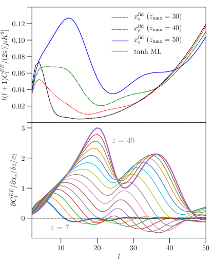
Figure 1: Top: $C_{\ell}^{EE}$ of fiducial models around which the PCs for $z_{\rm max}=30,40,50$ vary vs. the tanh chain maximum likelihood model. Bottom: Responses of the $C_{\ell}^{EE}$ spectrum to the ionization fraction at different redshifts (7 to 49 with spacing $\Delta z=3$). Responses are calculated per unit redshift from $\delta z=0.25$ perturbations around the fiducial $z_{\rm max}=50$ model and scaled to its cosmic variance per multipole. Note the similarity of the $\ell\lesssim 10$ responses for $z\gtrsim 10$ and differences at $\ell\gtrsim 15$ and $\ell\gtrsim 30$.

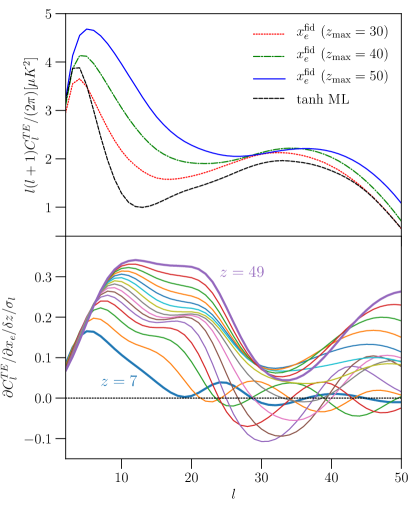
Figure 2: Same as Fig. 1 but for $C_{\ell}^{TE}$. Note again the similarity of the $\ell\lesssim 10$ responses for $z\gtrsim 10$.

The observable impact on the large-angle $E$-mode polarization spectrum of any ionization history out to a given $z_{\rm max}$ in the reionization range can be completely characterized to cosmic variance precision by just a few principal component parameters. We mainly follow Ref. Heinrich et al. (2017) for the PC construction but highlight the role of $z_{\rm max}$ and its relationship to features in the observable power spectra.

We begin by allowing arbitrary perturbations of the ionization fraction relative to the fully ionized hydrogen $x_{e}(z)$ around a fiducial model. Following Ref. Heinrich et al. (2017), the fiducial model is $x_{e}^{\rm fid}(z)=0.15$ in the range $z_{\rm min}<z<z_{\rm max}$ and vanishes for $z>z_{\rm max}$ (see example of $z_{\rm max}=30$ in Ref. Heinrich et al. (2017), Fig. 1). We take $z_{\rm min}=6$ and assume fully ionized hydrogen and singly ionized helium, $x_{e}^{\rm fid}(z)=1+f_{\rm He}$ for $z_{\rm He}\lesssim z<z_{\rm min}$, consistent with Ly$\alpha$ forest constraints (e.g. Becker et al. (2015)). Helium becomes fully ionized at $z_{\rm He}$, which is modeled here as a tanh function in redshift centered at $z_{\rm He}=3.5$ Becker et al. (2011) with width $\Delta z=0.5$. Therefore $x_{e}=1+2f_{\rm He}$ for $z\lesssim z_{\rm He}$. Here,

$$f_{\rm He}=\frac{n_{\rm He}}{n_{\rm H}}=\frac{m_{\rm H}}{m_{\rm He}}\frac{Y_{p}}{1-Y_{p}}$$ (1)

is the ratio of the helium to hydrogen number density, and $Y_{p}$ is the helium mass fraction, set to be consistent with big bang nucleosynthesis for the chosen baryon density. The $EE$ and $TE$ power spectra for the fiducial model with $z_{\rm max}=30,40,50$ are shown in Figs. 1 and 2 (upper panels).

These fiducial models differ substantially from each other and from the standard tanh or steplike reionization model

$$x_{e}^{\rm true}(z)=\frac{1+f_{\rm He}}{2}\left\{1+\tanh\left[\frac{y(z_{\rm re})-y(z)}{\Delta y}\right]\right\},$$ (2)

with $y(z)=(1+z)^{3/2}$, $\Delta y=(3/2)(1+z)^{1/2}\Delta z$, and $\Delta z=0.5$. This tanh model is also shown in Figs. 1 and 2 (black dashed) for the best fit $z_{\rm re}=9.85$ ($\tau=0.0765$) from Ref. Heinrich et al. (2017). Note in particular the very different shape of the $EE$ power spectrum which has a sharper peak at lower multipoles than all the fiducial models.

Next we consider variations around these fiducial models. In practice, we discretize $x_{e}(z)$ with a redshift spacing $\delta z=0.25$ so that each $x_{e}(z_{i})$ is a parameter. The full ionization history is constructed as the linear interpolation of these discrete perturbations. In Figs. 1 and 2 (lower panel), we display the observable responses to perturbations in $x_{e}(z_{i})$ around the $z_{\rm max}=50$ fiducial model through the derivatives $\partial C_{\ell}^{EE}/\partial x_{e}(z_{i})/\delta z$ and $\partial C_{\ell}^{TE}/\partial x_{e}(z_{i})/\delta z$ respectively. To highlight the ultimate observability of these variations, we scale the derivatives to the cosmic variance per $\ell$ mode

$$\sigma_{\ell}=\begin{cases}\sqrt{\frac{1}{2\ell+1}}\sqrt{C_{\ell}^{TT}C_{\ell}^{EE}+(C_{\ell}^{TE})^{2}},&TE;\\ \sqrt{\frac{2}{2\ell+1}}C_{\ell}^{EE},&EE.\\ \end{cases}$$ (3)

This scaling highlights the fact that most of the information on the ionization history will ultimately come from the $EE$ spectrum even though for the low signal to noise of the Planck polarization measurement $TE$ contributes as well.

Relatedly, by scaling to the cosmic variance rather than the Planck noise variance, we visually overweight the low signal-to-noise regions. For this reason when displaying the data and power spectrum differences, we also choose to calculate $\sigma_{\ell}$ with the fiducial model for $z_{\rm max}=50$ rather than the tanh model which has an even smaller signal. We retain this convention for the $z_{\rm max}=30,40$ cases so that power spectrum differences and data are displayed with the same convention. To compute power spectra, we use a modified version of CAMB Lewis et al. (2000); Howlett et al. (2012) and to calculate derivatives we use a double sided finite difference of fixed optical depth $\delta\tau\approx\pm 0.0006$ and 0.001 for $z_{\rm max}=40$ and 50 respectively to assure convergence and numerical stability. These derivatives are calculated at fixed $A_{s}e^{-2\tau}$ rather than fixed power spectrum normalization $A_{s}$ since the former is well constrained from the acoustic peaks. For $z_{\rm max}=30$, we follow the construction from Ref. Heinrich et al. (2017). For the calculation of derivatives we boost the accuracy of CAMB and use a small smoothing in $z$ for numerical stability and accuracy. For all other calculations we smooth the ionization history with a Gaussian in $\mathrm{ln}(1+z)$ of width $\sigma_{\mathrm{ln}(1+z)}=0.015$ which speeds up the analysis with negligible loss in precision for realistically smooth ionization histories.

First notice that to get substantial changes in $EE$ power at $\ell\gtrsim 10$, we require $z_{i}\gtrsim 10$. Note also that the relatively large features above $\ell\sim 15$ are influenced by the scaling to the cosmic variance of the fiducial model (see Fig. 1 top panel) and are in a regime which is not well measured by Planck. For $TE$, the contributions relative to cosmic variance look slightly smoother in multipole given the smooth temperature spectrum though again enhancements at $\ell\gtrsim 10$ require $z_{i}\gtrsim 10$.

Next notice that the various perturbations in $x_{e}(z_{i})$ at $z_{i}\gtrsim 15$ are very similar in $EE$ for the $\ell\lesssim 10$ regime that is constrained by the data. They differ more strongly in the low signal-to-noise region beyond $\ell\sim 15$. Given that the quadrupolar sources of polarization are associated with the horizon scale, the higher the redshift the higher the maximum multipole of the response but even high redshift perturbations affect $\ell\lesssim 10$. We shall see that this implies that the best measured regime does not provide a strong constraint on the specific redshift at which there is a preference for a finite high redshift ionization fraction. More detailed differentiation requires detections in the low signal regime.

The degenerate responses in the observables to neighboring $z_{i}$ are also what makes the PC parameterization much more efficient than a direct redshift space exploration. We construct the PCs as the eigenfunctions of the Fisher matrix of the $x_{e}(z_{i})$ perturbations for cosmic variance limited $C_{\ell}^{EE}$ measurements which, as discussed above, ultimately contain almost all of the low multipole information on reionization

$$F_{ij}=\sum_{\ell}\frac{1}{\sigma_{\ell}^{2}}{\partial C_{\ell}^{EE}\over\partial x_{e}(z_{i})}{\partial C_{\ell}^{EE}\over\partial x_{e}(z_{j})}=\sum_{a}S_{a}(z_{i})\sigma_{a}^{-2}S_{a}(z_{j}).$$ (4)

Note that in this construction, as opposed to the figures, $\sigma_{\ell}$ is the cosmic variance per multipole of the fiducial model in question rather than the fixed case of $z_{\rm max}=50$. We again linearly interpolate the discrete $S_{a}(z_{i})$ to obtain the continuous functions $S_{a}(z)$ and characterize the ionization history as

$$x_{e}(z)=x_{e}^{\rm fid}(z)+\sum_{a}m_{a}S_{a}(z),$$ (5)

where $m_{a}$ are the PC amplitudes.

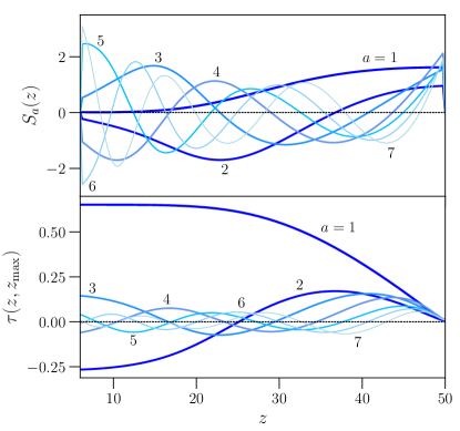
Figure 3: First $n_{\rm{PC}}=7$ PCs which form a complete basis for ionization histories up to $z_{\rm max}=50$ with respect to the large angle $C_{\ell}^{EE}$ observables. Top: Ionization PCs in redshift. Bottom: Cumulative optical depth for unit amplitude PCs. Higher PCs correspond to finer variations in redshift space which leave unobservable effects.

After obtaining $S_{a}(z)$ from Eq. (4), we rank order them from the smallest to largest variance $\sigma_{a}^{2}$. Then we determine $n_{\rm PC}$, the minimum number of PCs needed to completely describe the impact on $C_{\ell}^{EE}$ from any ionization history to cosmic variance limit Hu and Holder (2003). We find that $n_{\rm PC}$ = 5 suffices for $z_{\rm max}=30$ and 40, whereas $n_{\rm PC}=7$ is needed for $z_{\rm max}=50$, because of the larger amount of information contained in the larger redshift range that the CMB is able to probe. Note that despite the large differences in the fiducial models shown in Fig. 1, all three sets of PCs can describe the tanh model to the cosmic variance limit.

As an illustration, the first seven principal components for $z_{\rm max}=50$ are shown in the top panel of Fig. 3. The higher variance PCs correspond to faster oscillations in redshift space. Consequently their impact on the cumulative Thomson optical depth

$$\tau(z,z_{\rm max})=n_{\rm H}(0)\sigma_{T}\int_{z}^{z_{\rm max}}dz\frac{x_{e}(z)(1+z)^{2}}{H(z)},$$ (6)

is reduced and so $\tau(z,z_{\rm max})$ provides a better visualization of the constraints than $x_{e}(z)$. Here $n_{\rm H}(0)$ is the hydrogen number density at $z=0$ and $H(z)$ is the expansion rate. Note that in practice, the integral boundary in $\tau(z,z_{\rm max})$ goes slightly past the nominal $z_{\rm max}$ to capture the effect of smoothing $x_{e}$ beyond $z_{\rm max}$. In the lower panel of Fig. 3, we show this quantity for the individual PCs with unit amplitude $m_{a}=1$ and $z_{\rm max}=50$. Since the optical depth as a function of redshift controls the observable properties of the power spectra, we can see why the first few PCs contain most of the information for the Planck data.

III Reionization PC Constraints

We analyze the Planck data for PC parameterized reionization histories that are complete to $z_{\rm max}=40,50$ extending the $z_{\rm max}=30$ range in Ref. Heinrich et al. (2017), where the details of the procedure are covered. In brief, we use the Planck public likelihoods plik_lite_TTTEEE for high-$\ell$’s and lowTEB for low-$\ell$’s, which includes the 2015 LFI but not HFI polarization Aghanim et al. (2015). To sample the posterior distribution of the PC amplitudes $m_{a}$, we use the Markov Chain Monte Carlo (MCMC) technique with a modified version of COSMOMC Lewis (2013); Lewis and Bridle (2002). We also marginalize the standard $\Lambda$CDM cosmological parameters: baryon density $\Omega_{b}h^{2}$, cold dark matter density $\Omega_{c}h^{2}$, effective acoustic scale $\theta_{\rm MCMC}$, scalar power spectrum log amplitude $\mathrm{ln}(10^{10}A_{s})$ and tilt $n_{s}$. We fix the neutrino mass to one massive species with $m_{\nu}=0.06$eV.

Following Ref. Mortonson and Hu (2008b), we adopt flat priors on the PC amplitudes within the bounds of physicality for the ionization history. By requiring that $0\leq x_{e}\leq x_{e}^{\rm max}$, each PC amplitude individually must lie in the range $m_{a}^{-}\leq m_{a}\leq m_{a}^{+}$ where

$$m_{a}^{\pm}=\int_{z_{\rm min}}^{z_{\rm max}}dz\frac{S_{a}(z)[x_{e}^{\rm max}-2x_{e}^{\rm fid}(z)]\pm x_{e}^{\rm max}|S_{a}(z)|}{2(z_{\rm max}-z_{\rm min})},$$ (7)

and by requiring

$$\int_{z_{\rm min}}^{z_{\rm max}}dz(x_{e}(z)-x_{e}^{\rm fid})^{2}\leq(z_{\rm max}-z_{\rm min})(x_{e}^{\rm max}-x_{e}^{\rm fid})^{2},$$ (8)

their joint variation must satisfy

$$\sum_{a}m_{a}^{2}\leq(x_{e}^{\rm max}-x_{e}^{\rm fid})^{2}.$$ (9)

Here we take $x_{e}^{\rm max}=1+f_{\rm He}$ for fully ionized hydrogen and singly ionized helium.

These are necessary but not sufficient conditions for physical ionization models $0\leq x_{e}(z)\leq 1+f_{\rm He}$ for at most singly ionized helium. This is because the omitted components impact physicality even though they do not affect the observables. On the other hand, when testing physical models for reionization with the constraints on the PC amplitudes, neither this prior nor the unphysical models that it still allows matter Heinrich et al. (2017).

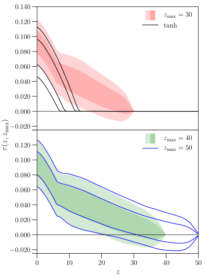
Figure 4: Cumulative optical depth $\tau(z,z_{\rm max})$ constraints (68% and 95% CL) for the various cases. Top: tanh (black lines) and PC chains with $z_{\rm max}=30$ (red bands). The functional form of the tanh model strongly disfavors optical depth at $z\gtrsim 15$ due to constraints on the total $\tau$ whereas PC constraints for $z_{\rm max}=30$ allow and even favor these contributions at $95\%$ CL. Bottom: same for $z_{\rm max}=40$ (green bands) and 50 (blue lines). Extending to higher redshift reveals a small amount of optical depth at $z=30$ ($\sim 1\sigma$ excess) missed in $z_{\rm max}=30$ analysis. This moves the $2\sigma$ point of excess from $z\sim 15$ in $z_{\rm max}=30$ to about $z\sim 20$ in both the $z_{\rm max}=40$ and 50 chains. The results are stable between the last two because of negligible contribution from $z\gtrsim 40$.

Table 1: Total and high redshift optical depth constraints for different analyses of Planck 2015 data.

Model	$z_{\rm max}$	$\tau(0,z_{\rm max})$	$\tau(15,z_{\rm max})$	$\tau(30,z_{\rm max})$
tanh	…	0.079 $\pm$ 0.017	…	…
PC	30	0.092 $\pm$ 0.015	0.033 $\pm$ 0.016	…
PC	40	0.095 $\pm$ 0.016	0.039 $\pm$ 0.017	0.013 $\pm$ 0.014
PC	50	0.096 $\pm$ 0.016	0.040 $\pm$ 0.018	0.016 $\pm$ 0.014

Since the meaning of the $m_{a}$ amplitudes themselves change with $z_{\rm max}$, we instead show the more robust and simple to interpret cumulative optical depth $\tau(z,z_{\rm max})$ (see Eq. 6). In Fig. 4, we plot the 68% and 95% confidence bands for the tanh model and PCs with $z_{\rm max}=30,40,50$. For the tanh model, optical depth at $z>15$ is strongly forbidden whereas in the other cases it is preferred at more than the 95% CL. As discussed in Ref. Heinrich et al. (2017), in the tanh model constraints on the total optical depth forbid a high redshift component due to its functional form not due to other properties of the data: ionization at high redshift must be accompanied by full ionization at all lower redshift. Relaxing this restriction with PCs out to $z_{\rm max}=30$ uncovers a $2\sigma$ preference of optical depth at $z>15$ Heinrich et al. (2017). Here, we show that these results are robust to further extending $z_{\rm max}$. In fact, the significance for $z>15$ in the $z_{\rm max}=30$ chains increases slightly from $2.1\sigma$ to $2.3\sigma$ in the $z_{\rm max}=40$ and 50 chains and there is a $\sim 1\sigma$ excess at $z\gtrsim 30$ (see Table 1). The point of $2\sigma$ excess moves from $z\sim 15$ to $z\sim 20$ and is stable between $z_{\rm max}=40$ and 50. This stabilization is related to the fact that there is no preference for ionization beyond $z\sim 40$.

Despite differences in redshift range ($z_{\rm max}=30-50$), number of PCs (5-7) and fiducial models around which the PCs are built, the constraints on the total optical depth remain consistent within the errors (see Table 1). This is especially notable since as the number of PCs and $z_{\rm max}$ increases, there is a larger prior volume for raising $\tau$ at high redshift compared with a choice of prior that is flat in $\tau$. Yet, unlike the WMAP data Mortonson and Hu (2008b), the Planck 2015 data themselves do not allow such variations (see Appendix A.1 for an extensive discussion). Conversely we caution the reader that PC constraints on $\tau$ are weak enough to still be subject to implicit and explicit priors from a given reionization model and should be interpreted in a model context for its impact on ionization source or other cosmological parameters. If these high redshift degrees of freedom are disfavored by the model, e.g. as in a population II scenario of reionization, then the PC constraints should be projected onto the model space with appropriate priors on the model parameters using the procedure in Ref. Heinrich et al. (2017) as illustrated in Miranda et al. (2017).

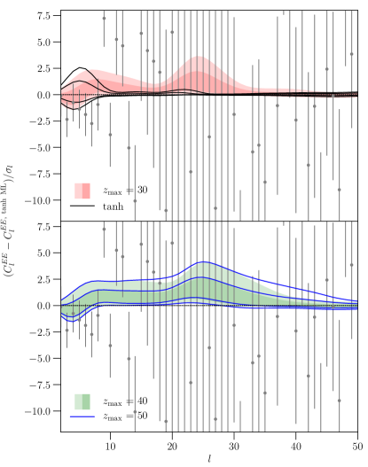
Figure 5: $EE$ data residuals and model posteriors with respect to the tanh maximum likelihood model scaled by the cosmic variance per multipole of the $z_{\rm max}=50$ fiducial model. Top: 68% and 95% CL posterior constraints from tanh (black lines) and PC chains with $z_{\rm max}=30$ (red bands). The high data point at $\ell=9$ and subsequent multipoles are generally better fit by PCs which allow for high redshift ionization. Bottom: same for $z_{\rm max}=40$ (green bands) and 50 (blue lines). Further increasing $z_{\rm max}$ produces similar fits around $\ell\sim 10$ and allow more freedom at $\ell\sim 15-20$ and $\ell\gtrsim 30$ where the data do not significantly constrain the models.

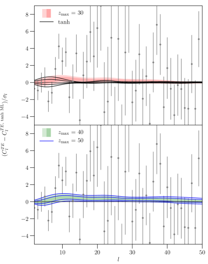
Figure 6: $TE$ data residuals and model posteriors as in Fig. 5. As with $EE$, the high data points around $\ell\sim 10$ allow for and favor high redshift ionization that is absent in the tanh model. The results in the well-constrained regions are again stable to $z_{\rm max}$.

To better understand the origin of the robustness of the high-$z$ ionization constraints to $z_{\rm max}$, we can compare the Planck $EE$ and $TE$ power spectrum data to the posterior probability distributions implied by the ionization constraints. In Figs. 5 and 6 respectively we show the 68% and 95% CL ranges for the tanh model compared to $z_{\rm max}=30$ and $z_{\rm max}=40$ to $z_{\rm max}=50$. We see that the main aspect of the data that tanh has difficulty explaining are the low $EE$ polarization points at $\ell\leq 8$ compared to the relatively high points that follow, especially $\ell=9$ Aghanim et al. (2015). The tanh ionization history cannot raise the latter without violating the constraints of the former. Furthermore the significance of this point in $TE$ is also increased due to a slightly low fluctuation in $TT$ there. On the other hand all 3 $z_{\rm max}$ cases produce very similar posteriors in the $\ell\lesssim 10$ range.

As we have seen in Fig. 1, raising the power at $\ell\sim 10$ requires ionization at $z>10$, but a wide range of redshifts have a similar impact there. The fit to the Planck data improves only very slightly with $z_{\rm max}=40$ by allowing more power between $\ell\sim 10-15$. Instead, the difference between the various $z_{\rm max}$ cases appears mainly at $\ell\gtrsim 15$ where the data do not yet significantly constrain the models. In particular the power spectra posteriors of $z_{\rm max}=40$ become more significantly distinguishable from $z_{\rm max}=30$ with a larger vertical range mainly at $\ell\sim 15-20$ (see Fig. 5). For the $\ell\gtrsim 30$ region, while the response functions in Fig. 1 imply systematically larger power there as a function of redshift, and the posteriors of Fig. 5 are different between all three $z_{\rm max}$, the Planck errors there are too large to have an impact on the models. Since these posterior differences are above the cosmic variance limit, they are in principle testable with future high precision ground or space based polarization measurements, especially should the true model have little ionization above $z_{\rm max}=30$.

Correspondingly the maximum likelihood models show improvements that support a $\sim 2\sigma$ preference for high redshift ionization mainly in the $\ell<30$ part of the likelihood. Note that the likelihood $\mathcal{L}$ reflects the goodness of fit of a particular set of parameters and is not sensitive to the prior chosen for the parameters unlike posterior constraints on $\tau$ and power spectra. Hence the preference for high-$z$ ionization is not simply due to the difference between flat priors on PCs and flat priors in $\tau$ as we explicitly demonstrate in Appendix A.1. In Table 2 we list the improvements of the best fit PC models over the tanh cases: for $z_{\rm max}=\{30,40,50\}$, $2\Delta\mathrm{ln}\mathcal{L}=\{5.5,5.9,6.1\}$ respectively (see also Hazra and Smoot (2017)). Note that for $z_{\rm max}=50$, this final further improvement is negligible despite having two additional PC parameters.

Robustness to $z_{\rm max}$ of these improvements further indicates that this mild preference for reionization histories beyond the tanh model really reflects a single aspect of reionization models: the presence of $z>10$ ionization. Hence this improvement should be considered as due to a single parameter in spite of the larger number of PCs and the wide range in redshift allowed in the analysis. We provide a concrete illustration of this single parameter in Appendix A.2. The number of PCs is chosen for completeness to the cosmic variance limit not because the additional parameters are required by the Planck data. This has the benefit that constraints on any model of reionization out to the same $z_{\rm max}$ can be directly obtained from the PC posteriors for Planck and for any future CMB experiment.

Conversely the $2\Delta\mathrm{ln}\mathcal{L}=5-6$ improvement does not provide a highly statistically significant detection of high-$z$ ionization on its own. In the context of models like the tanh case which disfavor high-$z$ ionization by an explicit or implicit modeling choice (see also Villanueva-Domingo et al. (2017)), this difference would simply be attributed to a statistical or systematic fluctuation. For models that do allow it (e.g. Ahn et al. (2012)), the high-$z$ ionization window is open and even mildly favored in the Planck 2015 polarization data due to features in the data at $\ell\sim 10$.

Table 2: Improvement of the Planck 2015 maximum likelihood $2\Delta\mathrm{ln}\mathcal{L}$ in different classes with respect to the tanh best-fit.

Model	$z_{\rm max}$	$2\Delta\mathrm{ln}\mathcal{L}$
tanh	…	0.0
PC	30	5.5
PC	40	5.9
PC	50	6.1
two step	…	5.3

IV Conclusion

In this work, we explored the relationship between signatures of high redshift ionization in CMB power spectra and features in the Planck 2015 LFI polarization data. We extend previous work by analyzing a complete parameterization of reionization to the cosmic variance limit out to $z_{\rm max}=40$ and $z_{\rm max}=50$ and identifying the specific aspect of the data that drive the constraints.

In a previous work with $z_{\rm max}=30$, we found a $2.1\sigma$ excess in cumulative optical depth at $z\sim 15$. In the $z_{\rm max}=40$ and 50 analyses, this excess is stable and in fact, slightly enhanced to $2.3\sigma$ because of the additional freedom to have optical depth at $z>30$. Beyond $z\approx 40$, however, there is no preference for finite ionization.

The origin and robustness of these results is related to data in the $\ell\sim 10$ region of the $EE$ and $TE$ power spectra. These data points are generally higher than can be accommodated by a reionization history with only $z<10$ ionization as in the steplike tanh model. Specifically, such models have difficulty simultaneously fitting the low power at $\ell\leq 8$ and abruptly higher power at $\ell=9$ simultaneously. Allowing for partial ionization out to $z>10$ through the PC basis can better accommodate the data. On the other hand the $\ell\lesssim 10$ region, which carries most of the signal to noise for Planck, cannot be used to discriminate the high redshift range further due to a near degeneracy in observational effects. Instead, differences appear at $\ell\sim 15-20$ and also at $\ell\gtrsim 30$. Though significant at the cosmic variance limit, for the Planck data the whole $\ell>10$ regime only provides a mild preference for $z\lesssim 40$.

These results are also consistently reflected in the moderate improvement of the maximum likelihood once high redshift ionization is accommodated with PC parameters: $2\Delta\mathrm{ln}\mathcal{L}$ of 5.5, 5.9 and 6.1 for $z_{\rm max}=30$, 40 and 50 respectively. These improvements are independent of the prior chosen for the parameters which is important since the PC approach entails a larger parameter volume for models with high redshift ionization than a flat prior on the total optical depth. This difference in prior volume is not relevant because the Planck 2015 data are more informative than the PC priors as we explicitly show in the Appendix.

The robustness of the results to $z_{\rm max}$ also indicates that these improvements should be viewed as originating from a single aspect of reionization models: the ability to accommodate $z>10$ ionization. The much larger number of PC parameters used in the actual analysis is chosen for completeness to the cosmic variance limit and not because they are required by the Planck data. These additional parameters are also not just artificially increasing the likelihood by fitting discrete noise fluctuations as the lack of further improvement of the likelihood with increased PC number or $z_{\rm max}$ shows. In the Appendix we provide a concrete example where the improvements are encapsulated into a single parameter for the high $z$ optical depth.

On the other hand, even if due to one single effective parameter, improvement at this level does not constitute strong evidence for high redshift ionization on its own. The benefit of the PC approach being complete to the cosmic variance limit is that any reionization model can be projected onto this basis without loss of information and interpreted with physically motivated priors. For models which accommodate high redshift ionization, a $z>10$ component is clearly allowed and even mildly preferred. Constraints on the total optical depth assuming a tanh model should not be used to exclude high redshift ionization in these models. Within a model class that forbids high redshift ionization, the poor fits would be attributed to a $2\sigma$ statistical fluctuation or systematic effects. Since the data are far from the cosmic variance limit, better measurements especially at $\ell=15-20$ and at $\ell>30$ can potentially decide this issue due to the excess power that high redshift ionization predicts there.

Indeed, the Planck team has done substantial work following the 2015 release on removing systematics from the low multipole measurements from the much more sensitive HFI measurements Aghanim et al. (2016). In particular, the 2016 intermediate release included a tanh analysis reporting a lower value of $\tau=0.055\pm 0.009$. As the tanh analysis provides essentially a low-$z$ estimate of optical depth, the high-$z$ component still remains unconstrained in this analysis. After this work was largely complete, Ref. Millea and Bouchet (2018) analyzed the 2016 intermediate release with principal components and found tighter constraints on the high-$z$ component. However, these data are still proprietary and the final full data set will soon be released publicly. In this context, our study of how features in the data translate to features or constraints on reionization at high redshift is valuable in determining the optimal strategy for extracting the most information from this and any future CMB data set.

Appendix A Optical depth parameters

A.1 How to (and not to) flatten the $\tau$ prior

After this work was largely complete, a concern was raised in Ref. Millea and Bouchet (2018) (hereafter MB18) regarding the $\tau$ prior implied by projecting the multidimensional flat PC prior onto that single dimension. MB18 claimed that since this prior is not flat in $\tau$, it leads to a bias in the PC result. In addition, MB18 proposed flattening the prior by multiplying by its inverse point-by-point in the multidimensional PC space and claim to show that flattening removes a large fraction of the shift of the $\tau$ posterior between tanh and PC results. We point out in this appendix that this logic is flawed and that even with a flat prior in $\tau$ the preference for a high redshift component remains.

When applied to datasets that are actually informative in the original multidimensional space, the MB18 approach to flattening actually introduces rather than removes bias. The problem is that it weights regions of the parameter space that are allowed by the original prior but rejected by the data and thus creates a new prior that is not locally flat across the region of support for the posterior. Their technique should only be applied to data that is informative solely on $\tau$, or more generally the parameter whose projected prior is flattened, and not on any of the other parameters in the space.

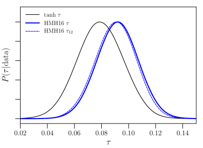
Figure 7: Posteriors of $\tau$ constructed from the complete 5 PCs (solid blue) vs. the first two PCs $\tau_{12}$ (Eq. 11) (dashed blue), both constructed with the physical prior of HMH16. The difference between them are very small compared to the relevant shifts discussed in this appendix, especially the shift between the tanh (black) and PC results.

To illustrate this explicitly in the context critiqued by MB18, we consider the case of the $z_{\rm max}=30$ analysis from HMH16 Heinrich et al. (2017). The total optical depth is a linear combination of contributions from the individual PCs

$$\tau=\tau_{\rm fid}+\sum_{a}m_{a}\tau_{a}$$ (10)

where $\tau_{a}$ is the optical depth for a unit amplitude PC and $\tau_{\rm fid}$ is the optical depth of the fiducial model. This linearity already indicates that if a given model parameterizes a linear trajectory in the PC space, then a flat prior on $m_{a}$ produces a flat prior in $\tau$ (see HMH16 for the tanh trajectory). This is the key to understanding why the flat prior on $m_{a}$ is compatible with a prior on $\tau$ that is locally flat.

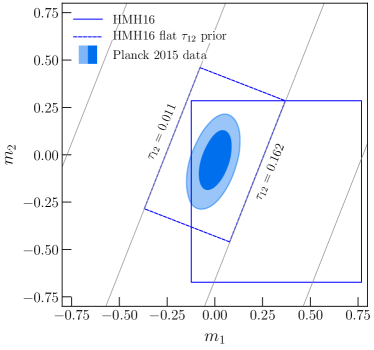
Figure 8: Priors on the $m_{1}-m_{2}$ parameter space: the original HMH16 prior (inset square, solid lines) and a prior that is flat in both $\tau_{12}$ and $m_{1}-m_{2}$ (rotated rectangle, dashed lines) whose sides are aligned with lines of constant $\tau_{12}$ (light gray lines). The HMH16 prior allows more parameter space at high vs low $\tau_{12}$ but this is not relevant since the data constraints (ellipses) exclude this region. In the allowed region, the only difference is that the HMH16 prior clips the low $m_{1}$ edge of the allowed region due to physicality and the assumption that reionization occurs at $z\geq 6$.

In the HMH16 case, almost all of the PC contribution to $\tau$ comes from the first two components

$$\tau_{12}=\tau_{\rm fid}+m_{1}\tau_{1}+m_{2}\tau_{2}\approx\tau.$$ (11)

In Fig. 7 we show that the posteriors for $\tau_{12}$ and $\tau$, both with the original HMH16 priors from Eq. (7) and (9), differ very little compared to the shift from the tanh model and likewise to any other relevant shifts discussed below.

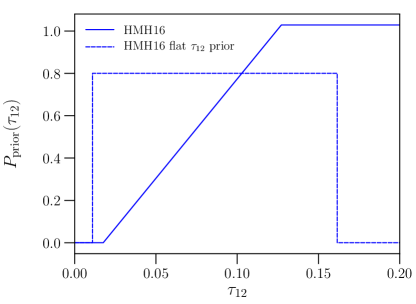
Figure 9: The integrated $\tau_{12}$ priors implied by the $m_{1}-m_{2}$ priors shown in Fig. 8: the HMH16 prior (solid line) is not flat due to the larger prior volume at high $\tau_{12}$ whereas the flat $\tau_{12}$ prior (dashed-line) is a flat top hat by construction. These two priors appear in projection to be quite different but locally in the region allowed by the data in Fig. 8 are almost the same.

By focusing the analysis on $\tau_{12}$, we can easily analyze purported biases from the PC priors. In Fig 8, we show the HMH16 priors on the $m_{1}-m_{2}$ space as the inset square (solid lines). Lines of constant $\tau_{12}$ are diagonal lines (light gray lines). As in MB18, we can project the HMH16 prior onto the $\tau_{12}$ direction. The result is the non-flat prior in $\tau_{12}$ shown in Fig. 9 (solid line). This shape can be easily understood as the length of the line segments of the constant $\tau_{12}$ lines that lie within the HMH16 prior box in Fig. 8. Note that the prior in Fig. 9 linearly rises with $\tau_{12}$ in the region of support of the posterior in Fig. 7 leading MB18 to claim a biased prior. However the Planck 2015 data is more informative than the prior in both $m_{1}$ and $m_{2}$ (Fig. 8, ellipses) making this elongation of the line segments at high $\tau_{12}$ irrelevant for the posterior.

By following the MB18 procedure of inverting this prior by multiplying each point in the PC sample by $P^{-1}_{\rm prior}[\tau_{12}(m_{1},m_{2})]$, we reproduce their results of a shift to lower $\tau_{12}$ for the posterior in Fig. 10. However this result occurs because the inversion weights the prior volume in regions that are not supported by the data and hence produces a bias against high $\tau_{12}$ in the region that is supported by the data, i.e. it makes the $\tau_{12}$ prior globally flat when integrated over the whole prior volume by making it locally not flat across the allowed region.

To make this point even more clear, we can explicitly construct a prior that is locally flat in both $m_{1}-m_{2}$ and $\tau_{12}$. Consider the rotated box shown in Fig 8 (dashed lines). Now the edges of the box are lines of minimum and maximum $\tau_{12}$ and the parameter orthogonal to $\tau_{12}$. As shown in Fig. 10 (dashed line), this new prior is explicitly flat in $\tau_{12}$ between its minimum and maximum. In Fig. 10, we show that the posterior from around its maximum out to high $\tau_{12}$ shifts negligibly between this new flat $\tau_{12}$ prior and the original HMH16 prior. The main impact is a slight enhancement at very low $\tau_{12}$ over the HMH16 results. This is because the HMH16 prior takes into account physicality constraints and restricts hydrogen to be fully ionized at $z\leq 6$. As shown in Fig. 8, this prior slightly clips the 95% CL region of the PC posterior at low $m_{1}$. This effect is qualitatively similar to what would occur in a tanh model if we restrict the redshift of reionization to $z>6$ (see also Fig. 12). Note also that this effect is much smaller than the bias that results from applying the MB18 procedure. We have also explicitly checked that changing the size of the rotated prior box does not affect the posterior within its region of support unless the box begins to exclude this region. Similarly, the $\tau(15,z_{\rm max})$ significance does not change much between the HMH16 and the flat $\tau_{12}$ prior result: $\tau(15,z_{\rm max})=0.033\pm 0.016$ and $\tau(15,z_{\rm max})=0.032\pm 0.018$ respectively.

We conclude that the MB18 procedure should not be applied to the Planck 2015 data set or any future measurement where the data is actually more informative than the physicality prior. It is nonetheless equally important to bear in mind that the weak preference for high-$z$ ionization in Planck 2015 data can still be outweighed by stronger explicit or implicit priors on the detailed astrophysics behind reionization as discussed in the main text.

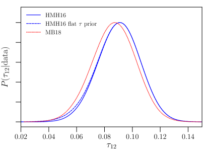
Figure 10: The $\tau_{12}$ posterior obtained using the HMH16 prior (solid blue) is nearly identical to that of the flat $\tau_{12}$ prior (dashed blue) except for the low-$\tau_{12}$ tail. This difference is the result of assuming reionization occurs at $z\geq 6$ and the physicality constraints of HMH16. The flattening procedure of MB18, on the other hand, introduces a bias shifting the entire posterior toward lower-$\tau_{12}$ due to the weight it places on regions allowed by the prior but forbidden by the data.

A.2 Adding a single high-$z$ $\tau$ parameter

Here we provide a concrete example of how the improved fit by the PC over tanh analysis, represents only one single aspect of the model – high-$z$ optical depth. Even though in the PC analysis, each ionization history is parametrized by 5 mode amplitudes for $z_{\rm max}=30$, the improvement can be encapsulated into a single additional parameter. This example demonstrates that the extra PC parameters in the analysis are included for completeness and are not just improving the likelihood incrementally by fitting random statistical fluctuations.

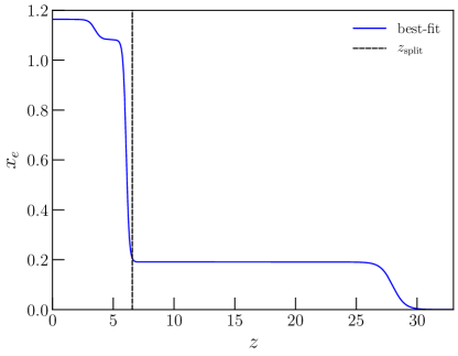
Figure 11: Best-fit two-step model (blue solid) with $\tau_{\rm lo}=0.040$ and $\tau_{\rm hi}=0.053$. The dashed black line shows the split used to define high vs low-$z$.

Our example is a two-step model

$$x_{e}^{\rm true} (z) \,=\frac{1+f_{\rm He}-x_{e}^{\rm min}}{2}\left\{1+\tanh\left[\frac{y(z_{\rm re})-y(z)}{\Delta y}\right]\right\}$$ (12)

$$+ \frac{x_{e}^{\rm min}-x_{e}^{\rm rec}}{2}\left\{1+\tanh\left[\frac{z_{\rm t}-z}{\Delta z_{2}}\right]\right\}+x_{e}^{\rm rec},$$

where $y(z)=(1+z)^{3/2}$, $\Delta y=(3/2)(1+z)^{1/2}\Delta z_{1}$, with $\Delta z_{1}=0.25$ instead of the usual $\Delta z_{1}=0.5$, to provide sharper distinctions between the two steps. We choose the second step to have $z_{\rm t}=28$ and $\Delta z_{2}=1.0$ to illustrate below how the 5 PC analysis with $z_{\rm max}=30$ represents the same model. Here $x_{e}^{\rm rec}$ is the ionization history from recombination only. The canonical tanh model is essentially recovered in the limit $x_{e}^{\rm min}$ approaches the negligible $x_{e}^{\rm rec}$. Therefore the double step model adds a single parameter to control the high-$z$ ionization plateau for $z_{\rm re}\lesssim z\lesssim z_{t}$. We show an example of the two-step model in Fig. 11.

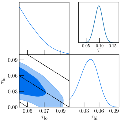
Figure 12: Low and high $z$ optical depth constraints from a two-step model that allows for high-redshift optical depth $\tau_{\rm hi}$. This component is detected at about $2\sigma$ significance. Dashed lines are lines of constant total $\tau=0.05,0.1$ and 0.15 and the implied $\tau$ posterior is shown in the upper right panel. Notice that the prior $\tau_{\rm low}\geq 0.04$ $(z_{\rm rei}\gtrsim 6$) suppresses the low $\tau$ tail by truncating its contributions (cf. Fig. 7, tanh model).

As in the previous section, we also illustrate our results using priors that are locally flat in $\tau$ but now divided into a low and high $z$ component by the double step. We therefore take as MCMC parameters $\tau_{\rm lo}(z_{\rm re},x_{e}^{\rm min})$ and $\tau_{\rm hi}(z_{\rm re},x_{e}^{\rm min})$, defined as Eq. (6) but with boundaries [0, $z_{\rm split}$] and [$z_{\rm split}$, $\infty$] respectively, such that the total $\tau=\tau_{\rm lo}+\tau_{\rm hi}$. We choose $z_{\rm split}=z_{\rm re}+2\Delta z_{1}$ to be conservative on the preference for $\tau_{\rm hi}$ in the data (see Fig. 11). We sample the posterior of $\tau_{\rm lo}$ and $\tau_{\rm hi}$ assuming a uniform prior in the intervals [0.04, $\tau_{\rm max}$] and [0, $\tau_{\rm max}$] respectively where $\tau_{\rm max}=0.35$; we also limit the total $\tau$ to $[0,\tau_{\rm max}]$.

Fig. 12 shows the posterior distribution of $\tau_{\rm lo}$ and $\tau_{\rm hi}$. Here $\tau_{\rm hi}=0.040\pm 0.017$ and is detected at about $2\sigma$ level similar to the PC result for $\tau(15,z_{\rm max})$. Likewise the best-fit two-step model ($\tau_{\rm lo}=0.040,\tau_{\rm hi}=0.053$) provides an improvement of $-2\Delta\ln{\cal L}=5.3$ over the best fit single-step tanh model whereas the best-fit PC parameters yields $5.5$ for $z_{\rm max}=30$. In the two-step model this improvement comes from a single extra parameter $\tau_{\rm hi}$. The posterior distribution of $\tau=\tau_{\rm lo}+\tau_{\rm hi}$ is also consistent with the shift between the tanh model and the PC posterior shown in Fig. 7.

One can further check that the $z_{\rm max}=30$ PC projection of the best-fit two-step model gives the same results as the direct method. The PC parameters of the model are $m_{1..5}=\{0.010,-0.035-0.009,-0.030,-0.005\}$. The difference in the total optical depth between the direct result and the PC projection is $\delta\tau=8\times 10^{-4}$, which is well below the errors in $\tau$. Once this insignificant difference is accounted for by scaling $A_{s}$ to a fixed $A_{s}e^{-2\tau}$, the difference in likelihood between the PC projected model and the direct model is $2\delta\ln{\cal L}=0.07$.

This two-step example highlights the fact that we include the 5 PC parameters to ensure that they can describe the polarization spectrum for any ionization history with $z<z_{\rm max}$ even if in the given model there really is only one extra effective parameter causing the likelihood differences from the tanh model. This supports our claim in the main text that these likelihood differences do not simply represent the overfitting of random statistical fluctuations multipole to multipole with multiple parameters. This example also addresses the question raised by MB18 of whether the remaining unphysical models allowed by the HMH16 priors bias results. In this case, the prior is both locally flat in $\tau$ parameters and explicitly allows only models with positive ionization.