Unique Spin Vortices in Quantum Dots with Spin-orbit Couplings

Abstract

Spin textures of one or two electrons in a quantum dot with Rashba or Dresselhaus spin-orbit couplings reveal several intriguing properties. We show that even at the single-electron level spin vortices with different topological charges exist. These topological textures appear in the ground state of the dots. The textures are stabilized by time-reversal symmetry breaking and are robust against the eccentricity of the dot. The phenomenon persists for the interacting two-electron dot in the presence of a magnetic field.

A variety of topological states have recently been observed in condensed matter physics. These novel states of matter are a direct consequence of spin-orbit coupling (SOC) TP01 ; TP02 with topological insulators (TIs) being one of the most prominent examples TP03 ; TP04 . The SOC also plays an important role in tailoring topological superconductors (TSs) where the elusive Majorana fermions might be present Mj01 ; Mj02 ; Mj03 . Both TIs and TSs display a topologically non-trivial structure in momentum space. SOC can, however, also lead to topological charges in real space. The Dzyaloshinskii-Moriya interaction DM01 ; DM02 —microscopically based on the SOC—can, for example, give rise to spin skyrmions in helical magnets sky01 ; sky02 and pseudospin skyrmions in bilayer graphene bilayerg . Synthetic spin-orbit couplings can also be engineered in cold atomic gases and skyrmion-like spin textures have been observed STB01 ; STB05 .

Quantum dots (QDs) are of practical and fundamental interest and provide an excellent platform to control the spin and charge of a single electron QD00 ; QD01 ; QD02 ; QD03 ; QD04 ; QD05 ; QD06 ; QD07 . Extensive studies on QDs with SOCs have been reported in recent years QDSOC01 ; QDSOC02 ; QDSOC03 ; QDSOC04 ; QDSOC05 ; QDSOC06 ; QDSOC07 ; QDSOC08 ; QDSOC09 ; QDSOC10 ; QDSOC11 ; siranush ; QDSOC12 ; QDSOC13 ; QDSOC14 ; QDSOC15 ; QDSOC16 . Furthermore, a Berry connection Berr in momentum space induced by the SOC has been studied QDSOC12 ; QDSOC13 .

In this letter, we investigate the spin textures associated with the electron density profiles in isotropic and elliptical QDs. We show that in the presence of SOC the in-plane spin texture of a single electron is a spin vortex. The QD is consequently turned into an artificial atom maksym with topological features. Spin vortices often emerge in many-spin systems forming either a crystalline arrangement or vortex/anti-vortex pairs vor01 ; vor02 . For instance, in quantum Hall systems the skyrmion is a single-particle excitation in low Landau levels and the in-plane spin texture is similar to the one we find in a QD with SOC. The skyrmion excitations in the former case are, however, induced by Coulomb interactions Ezawa . In contrast, we show here that in a QD a single vortex can exist in the ground-state of a non-interacting quantum system.

We focus on the physics of the two-dimensional (2D) surface where the QD is constructed QD01 . We consider both the Rashba and the linear Dresselhaus SOCs which arise in materials with broken inversion symmetry. The strength of the Rashba SOC can be controlled by a gate electric field Rash01 ; Rash02 ; Rash03 ; Rash04 ; Rash05 . Moreover, the ratio of the Rashba SOC to the Dresselhaus SOC can be tuned over a wide range, for instance in InAs QDs, by applying an in-plane magnetic field Rash05 . We will show that this leads to a system where the topological charge can be dynamically controlled by external electromagnetic fields making spin vortices in QDs possible candidates for future spintronics and quantum information applications.

The SOCs can be theoretically considered as effective momentum-dependent magnetic fields SOC01 ; SOC02 ; SOC03 ; SOC04 . In the absence of a confinement and an external magnetic field, the momentum is conserved and the SOC in the Hamiltonian becomes a momentum-dependent operator with a good quantum number (e.g., the helicity operator for Rashba SOC). On the other hand, the spin state is momentum-independent if both Rashba and Dresselhaus couplings have equal strength and there is no Zeeman coupling, leading to a persistent spin helix shx01 ; shx02 ; shx03 . This particular spin state persists in the presence of a confinement potential and can be obtained by exactly solving the Hamiltonian which is equivalent to a quantum Rabi model supplement . If the spin is not a good quantum number then it is instructive to study the spin field in a given single-particle wavefunction $\Psi(\mathbf{r})$ of the dot

$$\sigma_{i}(\mathbf{r})=\Psi^{{\dagger}}(\mathbf{r})\sigma_{i}\Psi(\mathbf{r}),$$ (1)

where $\sigma_{i}$ for $i=x,y,z$ are Pauli matrices. An in-plane vector field $\bm{\sigma}(\mathbf{r})=\left(\sigma_{x}(\mathbf{r}),\sigma_{y}(\mathbf{r})\right)$ reveals how the spin in real space is locally affected by the effective magnetic field. In the following, we demonstrate that generic SOCs compel the spin field to rotate around the center of the QD and to develop into a spin vortex.

The Hamiltonian of an electron with effective mass $m^{\ast}$ and charge $-e$ in a quantum dot with SOCs is given by

$$H=\frac{\left(\mathbf{p+}e\mathbf{A}\right)^{2}}{2m^{\ast}}+\frac{m^{\ast}}{2}\left(\omega_{x}^{2}x^{2}+\omega_{y}^{2}y^{2}\right)+\frac{\Delta\sigma_{z}}{2}+H_{SOC},$$ (2)

where the vector potential is chosen in the symmetric gauge $\mathbf{A}=\frac{1}{2}B\left(-y,x,0\right)$ with the magnetic field $B$. The confinement is anisotropic with the frequencies in two directions, $\omega_{x}$ and $\omega_{y}$, and $\Delta$ is the Zeeman coupling. We consider both the Rashba SOC, $H_{R}$, and the Dresselhaus SOC, $H_{D}$, with

$$H_{R} = g_{1}\left(\sigma_{x}P_{y}-\sigma_{y}P_{x}\right),$$ (3)

$$H_{D} = g_{2}\left(\sigma_{y}P_{y}-\sigma_{x}P_{x}\right),$$ (4)

and $H_{SOC}=H_{R}+H_{D}$. $P_{i}=p_{i}+eA_{i}$ is the kinetic momentum, and $g_{1,2}$ determine the strength of each SOC. We note that Rashba and Dresselhaus terms have different rotational symmetry generators, $H_{R}$ commutes with $L_{z}+\hbar\sigma_{z}/2$ while $H_{D}$ commutes with $L_{z}-\hbar\sigma_{z}/2$, where $L_{z}$ is the $z$-component of the angular momentum operator. In the following, we will show that this difference is responsible for the different topological charges associated with the spin vortex of the dot.

It is also useful to introduce a renormalized set of frequencies $\Omega_{i}=\sqrt{\omega_{i}^{2}+\omega_{c}^{2}/4}$ with the cyclotron frequency $\omega_{c}=eB/m^{\ast}$. The natural length scales in $x$ and $y$ directions are $\ell_{i}=\sqrt{\hbar/(m^{\ast}\Omega_{i})}$ while the confinement lengths are defined as $R_{i}=\sqrt{\hbar/(m^{\ast}\omega_{i})}$. In the numerical calculations presented in the following the eigenvectors of $H_{0}=\frac{\mathbf{p}^{2}}{2m^{\ast}}+\frac{m^{\ast}}{2}\left(\Omega_{x}^{2}x^{2}+\Omega_{y}^{2}y^{2}\right)+\frac{\Delta}{2}\sigma_{z}$, which is a two-dimensional harmonic oscillator, are used as a basis set.

No analytical solution is known for the generic Hamiltonian in Eq. (2) due to its complexity ExSOC . We can, however, analytically investigate the special case of an isotropic dot ($\Omega_{x,y}=\Omega$, $\ell_{x,y}=\ell$) without a magnetic field and with equal SOCs, $g_{1,2}=g$. The Hamiltonian (2) is then equivalent to a two-component quantum Rabi model which has been extensively studied in quantum optics supplement . The ground states in this case are a degenerate Kramers pair due to time reversal symmetry,

$$\left|GS\right\rangle_{\pm}=\frac{1}{\sqrt{2}}e^{\pm i\sqrt{2}m^{*}\left(y-x\right)g/\hbar}\left(\begin{array}[]{c}\pm e^{-i\pi/4}\\ 1\end{array}\right)\left|0,0\right\rangle$$ (5)

where $\left|0,0\right\rangle$ is the ground state of the two-dimensional quantum oscillator $H_{0}$. A very weak magnetic field will lift the degeneracy of the Kramers pair, and the unique ground state is then given by $\left|GS\right\rangle=(\left|GS\right\rangle_{+}+\textrm{sgn}(\Delta)\left|GS\right\rangle_{-})/\sqrt{2}$ which minimizes the energy supplement . The spin fields are consequently well defined. We note some features of the spin field: (i) There is a mirror symmetry about the line $x=\pm y$. (ii) $\sigma_{x}(\mathbf{r})+\sigma_{y}(\mathbf{r})=0$, and $\sigma_{x}(\mathbf{r})=\sigma_{y}(\mathbf{r})=0$ along the line $x=y$. (iii) $\sigma_{z}(\mathbf{r})=-\frac{\textrm{sgn}(\Delta)}{\pi\ell^{2}}e^{-2x^{2}/\ell_{x}}\cos\left(4\sqrt{2}m^{*}xg/\hbar\right)$ along the line $x=-y$, i.e., $\sigma_{z}(\mathbf{r})$ is a spiral. Its period is related to the effective mass and the strength of the SOCs. We find that the exact solution perfectly agrees with the exact diagonalization results shown in Fig. 1.

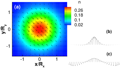
Figure 1: (Color online) Numerical results for a single-electron QD with $R_{x}=R_{y}=35$nm, $B=0.1$T, and equal SOCs $\hbar g_{1}=\hbar g_{2}=20$ nm$\cdot$ meV. (a) Electron density (contours) and in-plane spin fields (arrows), (b) $\sigma_{z}(\mathbf{r})$ along $x=-y$, and (c) the normalized $\tilde{\sigma}_{z}(\mathbf{r})=\sigma_{z}(\mathbf{r})/\sqrt{\bm{\sigma}(\mathbf{r})^{2}+\sigma_{z}(\mathbf{r})^{2}}$ along $x=-y$.

Similar results are found for the case $g_{1}=-g_{2}$. For large magnetic fields the exact solution for the case without field is no longer a good starting point and the spin texture starts to rotate supplement .

Next, we study the case of an isotropic dot in a weak magnetic field with generic strengths of the SOCs $g_{1}$ and $g_{2}$ based on a standard perturbative calculation. We find that the in-plane spin fields up to first order in $g_{1,2}$ are given by

$$\sigma_{x}(\mathbf{r}) = \xi(r)(r/\ell)\left(\bar{g}_{2}\sin{\theta}-\bar{g}_{1}\cos{\theta}\right),$$ (6)

$$\sigma_{y}(\mathbf{r}) = \xi(r)(r/\ell)\left(\bar{g}_{2}\cos{\theta}-\bar{g}_{1}\sin{\theta}\right),$$ (7)

and $\sigma_{z}(\mathbf{r})=\xi(r)/2$ with $\xi(r)=2e^{-r^{2}/\ell^{2}}/\pi\ell^{2}$, $\theta$ is the polar angle in coordinate space, and the new parameters are

$$\bar{g}_{1,2}=\frac{\hbar g_{1,2}}{\ell}\frac{1\pm\omega_{c}/(2\Omega)}{\hbar(\Omega\pm\omega_{c}/2)-\Delta},$$ (8)

where we have assumed $\Delta<0$. The in-plane spin field $\sigma(\mathbf{r})$ winds once around the origin and acquires a topological charge $q=\pm 1$ when $\bar{g}_{1}\neq\bar{g}_{2}$. If $\bar{g}_{1}=\bar{g}_{2}$, no vortex appears in agreement with the exact solution discussed earlier. If ${g}_{1}=0$ or ${g}_{2}=0$, $\sigma(\mathbf{r})$ obtained perturbatively qualitatively agrees with the numerical solutions shown in Fig. 2, and the vortices even exist in a strong magnetic field beyond the perturbation calculations.

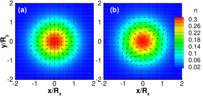
Figure 2: (Color online) Single-electron QD with $R_{x}=R_{y}=15$nm, $B=0.1$T ($\Delta<0$), and (a) Rashba SOC $\hbar g_{1}=40$ nm$\cdot$ meV only, and (b) Dresselhaus SOC $\hbar g_{2}=20$ nm$\cdot$ meV only.

We stress that the two vortex configurations are stable and representative for the regime $g_{1}\gg g_{2}$ and $g_{2}\gg g_{1}$, respectively supplement . We further note that under $B\to-B$ the spin field changes direction, $\sigma(\mathbf{r})\to-\sigma(\mathbf{r})$, leaving the topological charge invariant though.

Next, we analyze the rotational symmetry of the two types of SOCs in order to characterize the sign of the winding number. First, we consider the spin field of a dot when only the Rashba SOC is present. The spin field is then invariant under the rotation matrix

$$U_{R}(\vartheta)=\begin{pmatrix}\cos{\vartheta}&\sin{\vartheta}\\ -\sin{\vartheta}&\cos{\vartheta}\end{pmatrix},$$ (9)

for $\vartheta\in[0,2\pi]$, which is rooted in the rotational symmetry of a Rashba dot under the operator $L_{z}+\hbar\sigma_{z}/2$. Therefore, the in-plane spin rotates clockwise by $2\pi$ if we move around the center of the dot in a clockwise direction, and hence, its winding number is $q=+1$. On the other hand, the in-plane spin field of a dot with only Dresselhaus SOC being present, is invariant under the action of $U_{D}(\vartheta)=U_{R}(-\vartheta)$. Along the same line of reasoning, the in-plane spin field then rotates anticlockwise by $2\pi$ if we move around the center in a clockwise direction. Dresselhaus SOC thus leads to a winding number $q=-1$. In the absence of an external magnetic field $B$, Kramers degeneracy may cancel the spin textures, since there is a global $\pi$ phase difference between the pair. Hence, the vortices should be stabilized by breaking of time-reversal symmetry.

In summary, we find for the single-electron dot with $g_{1}=\pm g_{2}$ and without or in a very weak magnetic field, that the in-plane spin field does not form a vortex. There is, however, a spiral in $\sigma_{z}\left(\mathbf{r}\right)$ along the line $x=\mp y$. For dominant Rashba or Dresselhaus SOC, on the other hand, the exact diagonalization results clearly show the formation of spin vortices. Rashba SOC induces a vortex with topological charge $q=+1$ while the Dresselhaus SOC induces a vortex with $q=-1$. These topological charges associated with the spin textures are stabilized by time-reversal symmetry breaking and are robust against the ellipticity of the dot supplement . If the dot is strained, the topological features are not changed, since the spin textures originate from the SOCs of the material. The total $\langle\sigma_{z}\rangle$ in the presence of SOC is no longer constant as a function of the applied magnetic field and becomes more and more polarized with increasing magnetic field. In Fig. 3 we compare $\left\langle\sigma_{z}\right\rangle$ for different cases.

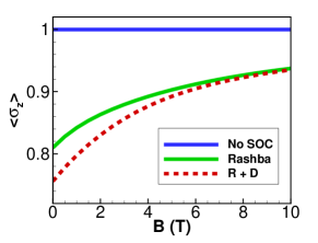
Figure 3: (Color online) The total $\left\langle\sigma_{z}\right\rangle$ in a single-electron dot ($R_{x}=R_{y}=15$nm) without SOC, with Rashba SOC only ($\hbar g_{1}=40$ nm$\cdot$ meV), and with both Rashba and Dresselhaus SOCs ($\hbar g_{1}=40$ nm$\cdot$ meV, $\hbar g_{2}=20$ nm$\cdot$ meV).

The distinct behavior of $\left\langle\sigma_{z}\right\rangle$ when SOCs are present might be observable experimentally via magnetometry or optically pumped NMR measurements sean ; private .

If there is more than one electron confined in the dot, we need to also consider the Coulomb interaction. The Hamiltonian of the interaction is given by $H_{C}=V\left(n_{1},n_{2},n_{3},n_{4}\right)c_{n_{1}}^{{\dagger}}c_{n_{2}}^{{\dagger}}c_{n_{3}}c_{n_{4}},$ where $c$ is the electron annihilation operator and $n_{i}=\left(n_{ix},n_{iy},n_{s}\right)$ is an index combining the quantum numbers of the two-dimensional oscillator in $x,y$ direction with the spin index. The interaction matrix elements are given in the Suppl. Mat. supplement . The full Hamiltonian with interaction is then $H_{I}=H+H_{C}$ with $H$ as given in Eq. (2). We diagonalize the interacting Hamiltonian exactly to obtain the electron and spin densities. Since the interacting system does contain very rich physics, we restrict the discussion in the following to the case of a dot with two electrons. To be concrete, we consider the case of an InAs dot here, where the effective mass is $m^{*}=0.042m_{e}$, Landé factor $g_{L}=-14$ and dielectric constant $\epsilon=14.6$. In this system it appears to be experimentally feasible to change the ratio of the SOCs $g_{1}/g_{2}$ over a wide range.

In a two-electron dot with Coulomb interactions, the spin textures can be much more complex than in the single-electron case. If there is no time reversal symmetry breaking, the texture is cancelled by the Kramers pair. In the presence of a magnetic field, the spin textures appear again with topological charge $+1$ or $-1$ if the dot is perfectly isotropic. For an anisotropic quantum dot the electron density will split into two centers in a strong magnetic field even without SOC. With SOCs the spin textures are modified by this density deformation. In the examples shown in Fig. 4, we find in both cases three vortices along the elongated $x$ axis.

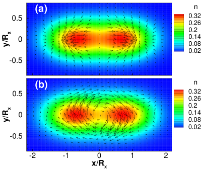
Figure 4: (Color online) The in-plane spin fields in an elliptic dot with two electrons, $R_{x}=15$nm, $R_{y}=10$nm at $B=5$T. The colors represent the electron density. (a) Rashba SOC only with $\hbar g_{1}=40$ nm$\cdot$ meV, and (b) Dresselhaus SOC only with $\hbar g_{2}=20$ nm$\cdot$ meV.

In the Rashba SOC case shown in Fig. 4(a) there are two vortices with $q=1$ and one with $q=-1$, while there are two vortices with $q=-1$ and one with $q=1$ in the Dresselhaus SOC case presented in Fig. 4(b). Hence, the total winding numbers are still $+1$ and $-1$ in a Rashba SOC and Dresselhaus SOC system, respectively, as in the single-electron dot. Indeed, the spin textures along the edges of the dot are quite similar to the single-particle case. Here interactions are less relevant and the spin textures are thus mainly induced by the SOCs.

In an isotropic two-electron dot with equal SOCs, $g_{1}=g_{2}$, we find that both the density profiles and spin textures undergo a dramatic change as a function of the applied magnetic field [Fig. 5].

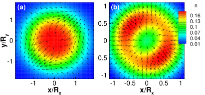
Figure 5: (Color online) The in-plane spin fields in a two-electron dot with $R_{x}=R_{y}=15$nm, and $\hbar g_{1}=\hbar g_{2}=20$ nm $\cdot$meV. The colors represent the electron density. (a) $B=3.5$T, topological charge $q=-1$, and (b) $B=18$T leading to $q=+1$.

In this case, the spin and density profiles are determined collectively by both the interactions and SOCs. For large magnetic fields we find, in particular, that the electron density splits mirror symmetrically along the line $x=y$ [Fig. 5(b)], causing also a complete rearrangement of the associated spin texture and a change of the total topological charge. This has to be contrasted with the case of an InAs dot without SOC where the angular momentum of the ground state changes from $L=-1$ to $L=3$ at about $B=17$T leading instead to a ring-shaped electron density. We further note that in a ZnO dot with stronger Coulomb interaction aram , the splitting of the electron density and the spin textures can be generated in a much lower magnetic field. Details will be published elsewhere. This splitting—which only occurs if both interactions and SOCs are present—could possibly be observed experimentally and would thus provide an indirect confirmation of a non-trivial spin texture in the dot.

In summary, we find that the combination of electron confinement and SOCs leads to vortex-like spin textures in the ground state even for a single-electron dot. The spin texture can be stabilized by an external magnetic field breaking the time-reversal symmetry. Interestingly, the winding number of the vortex is different for dots with dominant Rashba SOC or Dresselhaus SOC. This difference can be traced back to the different symmetries of the Hamiltonian. The Rashba SOC commutes with $L_{z}+\hbar\sigma_{z}/2$ leading to a topological charge of the spin field of $q=+1$ while the Dresselhaus SOC commutes with $L_{z}-\hbar\sigma_{z}/2$ and the topological charge is $q=-1$. Using the exact diagonalization scheme we have shown that these spin vortices do persist also in interacting multi-electron dots. For an elliptic two-electron dot we find, in particular, that more than one spin vortex can exist. In all investigated cases the total topological charge is, however, still $q=\pm 1$ as in the single-electron case. Physically, this is understood by noting that the spin configuration at the edge of the dot, where the electron density is low, is only weakly affected by the interactions. We thus conjecture that the total topological charge for a spin texture in multi-electron dots is always fixed to $q=\pm 1$.

The spin textures in QDs described in this letter are similar to the in-plane structure of (anti-)skyrmion excitations in quantum Hall systems. The locations of the skyrmions in a quantum Hall systems are, however, unknown making it difficult to observe a single skyrmion directly. The existence of skyrmions has so far only been confirmed indirectly by NMR and transport measurements. In contrast, the spin vortices in QD systems are localized at a known position. This might possibly open new avenues for spintronics and quantum information applications. Arrays of QDs have, for example, been realized experimentally KouwenhovenHekking ; PiqueroZulaica and have been considered as a potential platform for quantum computation LossDiVincenzo ; ZanardiRossi ; Awschalom ; Nowack . In such an array of QDs with SOCs the ratio of Rashba to Dresselhaus couplings might be tunable by gates over a sufficiently wide range to realize a system with localized and controllable topological charges $q=\pm 1$. At a minimum, such a setup would allow for an indirect probe of the spin texture by measuring the field dependence of the out-of-plane spin component [Fig. 3], either by a magnetometer or in an NMR experiment private .

We acknowledge useful discussions with Sean Barrett (Yale). TC acknowledges support by the Canada Research Chairs Program of the Government of Canada. JS acknowledges support by the Natural Sciences and Engineering Research Council (NSERC, Canada) and by the Deutsche Forschungsgemeinschaft (DFG) via Research Unit FOR 2316. Computation time was provided by Calcul Québec and Compute Canada.

Unique Spin Vortices in Quantum Dots with Spin-orbit Couplings – Supplemental material
Wenchen Luo, Amin Naseri, Jesko Sirker, and Tapash Chakraborty

In the supplemental material we present details of the analytical calculations for the single-electron parabolic quantum dot (QD) fock ; darwin ; QD_book and additional numerical data demonstrating the stability of the topological spin textures described in the letter. In Sec. 1 the derivation of the exact eigenstates for a single-electron dot with equal Rashba and Dresselhaus spin-orbit couplings (SOCs) and without the magnetic field, as well as the lifting of the Kramers degeneracy for small fields are discussed. In Sec. 2 we present additional numerical data for the single-electron QD showing that (i) for large magnetic fields and $g_{1}=g_{2}$ the spin texture starts to rotate, (ii) the topological charges are robust in the cases $g_{1}\gg g_{2}$ and $g_{2}\gg g_{1}$ and similar to the spin textures with Rashba or Dresselhaus coupling only discussed in the main text, and (iii) the topological charges are also robust against straining of the QD. In Sec. 3 we give explicit formulas for the Coulomb matrix elements for multi-electron QDs.

I 1. Single-electron dot: Equal Rashba and Dresselhaus couplings

The Hamiltonian of an electron in an isotropic dot $\Omega_{x,y}=\Omega$, $\ell_{x,y}=\ell$ and $g_{1}=g_{2}=g$ without magnetic field is equivalent to a two-component quantum Rabi model. In this case the Hamiltonian (2) in the main text reads,

$$H=\frac{\mathbf{p}^{2}}{2m^{\ast}}+\frac{1}{2}m^{\ast}\omega^{2}\left(x^{2}+y^{2}\right)-\left(p_{x}-p_{y}\right)g\left(\sigma_{x}+\sigma_{y}\right).$$ (10)

We now define the ladder operators of the quantum harmonic oscillator

$$a_{\mu} = \sqrt{\frac{m^{\ast}\omega}{2\hbar}}\left(\mu+\frac{i}{m^{\ast}\omega}p_{\mu}\right),$$ (11)

and use $a_{x}=-ib_{x},a_{y}=ib_{y},$ to transform the Hamiltonian to

$$H=b_{x}^{{\dagger}}b_{x}+b_{y}^{{\dagger}}b_{y}+G\left(b_{x}^{{\dagger}}+b_{x}+b_{y}^{{\dagger}}+b_{y}\right)\frac{1}{\sqrt{2}}\left(\sigma_{x}+\sigma_{y}\right),$$ (12)

where $G=g\sqrt{\hbar m^{\ast}\omega}$. Then, performing a unitary transformation

$$U = \frac{1}{\sqrt{2}}\left(\begin{array}[]{cc}1&e^{-i\pi/4}\\ e^{i\pi/4}&-1\end{array}\right),$$ (15)

leads to

$$UHU^{{\dagger}} = b_{x}^{{\dagger}}b_{x}+b_{y}^{{\dagger}}b_{y}+G\left(b_{x}^{{\dagger}}+b_{x}+b_{y}^{{\dagger}}+b_{y}\right)\sigma_{z},$$ (16)

which is a two-component quantum Rabi model with zero splitting rabi . The case of $g_{1}=-g_{2}$ can be solved in a similar manner.

In the main text, we show in Eq. (5) that the ground states are a degenerate Kramers pair. If the magnetic field is infinitesimal then the degeneracy is lifted. Since ${}_{\pm}\left\langle GS\right|L_{z}\left|GS\right\rangle_{\pm}=0$, the unique ground state can be found to lowest order by minimizing the Zeeman energy only. We use the ansatz

$$\left|GS\right\rangle=A\left|GS\right\rangle_{+}+B\left|GS\right\rangle_{-}.$$ (17)

with coefficients $A,B$. The Zeeman energy is then proportional to

$$\left\langle GS\right|\Delta\sigma_{z}\left|GS\right\rangle = -\Delta\int^{\infty}_{-\infty}dxdy\left(AB^{\ast}e^{-i2\sqrt{2}g\ell\frac{m^{*}}{\hbar}\left(x-y\right)}+A^{\ast}Be^{i2\sqrt{2}g\ell\frac{m^{*}}{\hbar}\left(x-y\right)}\right)e^{-x^{2}-y^{2}}$$ (18)

$$= -\Delta\left(AB^{\ast}+A^{\ast}B\right)\pi e^{-4\left(g\ell\frac{m^{*}}{\hbar}\right)^{2}}.$$

For $\Delta>0$ the minimization of the Zeeman energy requires $A=B=\frac{1}{\sqrt{2}}$ while it requires $A=-B=\frac{1}{\sqrt{2}}$ for $\Delta<0$. Hence,

$$\left|GS\right\rangle=\frac{\left|GS\right\rangle_{+}+\textrm{sgn}\left(\Delta\right)\left|GS\right\rangle_{-}}{\sqrt{2}}.$$ (19)

The other calculations presented in the main text are the standard first-order perturbative calculations.

II 2. Single-electron dot: Numerical results

In Fig. 1(a) of the main text we have shown that the in-plane spin texture in a weak magnetic field for the case $g_{1}=g_{2}$ is mirror symmetric around the line $x=y$, consistent with the perturbative calculation. For larger fields the perturbative ground state given above is, however, no longer a good starting point. In Fig. 6, we show how the in-plane spin textures evolve with increasing magnetic field.

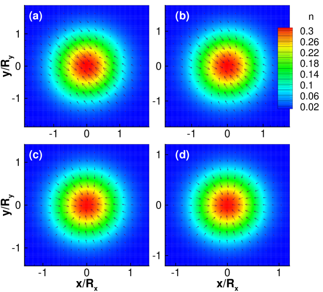
Figure 6: (Color online) The in-plane spin field with $\hbar g_{1}=\hbar g_{2}=20$ nm$\cdot$ meV in a single-electron dot with $R_{x}=R_{y}=15$nm at magnetic fields (a) $B=3$T, (b) $B=5$T, (c) $B=10$T, and (d) $B=15$T.

All these results show a mirror symmetry about the line $x=\pm y$. However, when the magnetic field becomes stronger the spins start to rotate leading to a spin texture similar to the case of Rashba SOC only. Note that the in-plane spin components are weaker than in the Rashba case though because the spin becomes more and more polarized along the $z$-direction.

In Fig. 2 of the main text we have shown the spin vortices in a single-electron dot if only the Rashba or the Dresselhaus SOC is present. In Fig. 7 we show that these results are indeed representative for the regimes $g_{1}\gg g_{2}$ and $g_{2}\gg g_{1}$.

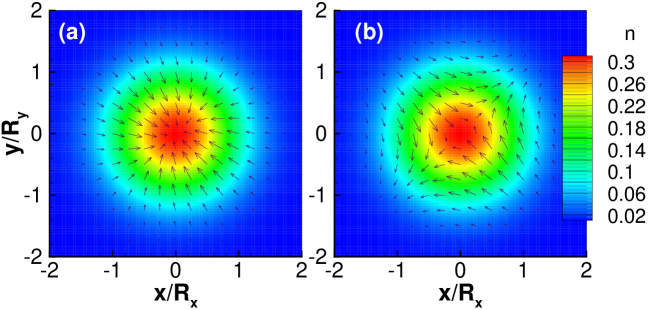
Figure 7: (Color online) The in-plane spin field in an isotropic single-electron dot with $R_{x}=R_{y}=15$nm at $B=0.1$T. The SOCs are (a) $\hbar g_{1}=20$ nm$\cdot$ meV and $\hbar g_{2}=5$nm$\cdot$ meV, and (b) $\hbar g_{1}=5$nm$\cdot$ meV and $\hbar g_{2}=20$nm$\cdot$meV.

We also note that even for larger magnetic fields the topological properties are not changed, although the spin textures are weakened. States with higher topological charge $|q|>1$ may exist in the excited states. Contrary to the spin textures in the ground state they are, however, fragile due to their Kramers partner.

Finally, we also show that the spin texture is robust against the eccentricity of the dot. We consider an elliptical InAs dot with $R_{x}=15$nm and $R_{y}=10$nm. From Fig. 8 it is obvious that the distortion of the dot does not qualitatively change the structure of the spin vortex.

Figure 8: (Color online) The in-plane spin field in a single-electron dot with $R_{x}=15$nm, $R_{y}=10$nm in $B=0.1$T. The SOCs are (a) $\hbar g_{1}=20$ nm$\cdot$ meV and $\hbar g_{2}=0$, and (b) $\hbar g_{1}=0$ and $\hbar g_{2}=20$nm$\cdot$meV.

III 3. Multi-electron dots: Coulomb interaction matrix elements

Below we explicitly display the Coulomb interaction matrix elements QD_book used in the exact diagonalization method for multi-electron dots

$$V\left(n_{1},n_{2},n_{3},n_{4}\right) = \frac{2}{\pi}\frac{e^{2}}{\epsilon\sqrt{\ell_{x}\ell_{y}}}\phi\left(n_{1x},n_{4x}\right)\phi\left(n_{1y},n_{4y}\right)\phi\left(n_{2x},n_{3x}\right)\phi\left(n_{2y},n_{3y}\right)$$

$$\left(-1\right)^{\left|n_{2x}-n_{3x}\right|+\left|n_{2y}-n_{3y}\right|}i^{\left|n_{1x}-n_{4x}\right|+\left|n_{1y}-n_{4y}\right|+\left|n_{2x}-n_{3x}\right|+\left|n_{2y}-n_{3y}\right|}$$

$$\int_{0}^{\infty}dxdy\,\Phi\left(n_{1x},n_{4x},x\right)\Phi\left(n_{2x},n_{3x},x\right)\frac{\Phi\left(n_{1y},n_{4y},y\right)\Phi\left(n_{2y},n_{3y},y\right)}{\sqrt{\frac{\ell_{y}}{\ell_{x}}x^{2}+\frac{\ell_{x}}{\ell_{y}}y^{2}}}.$$

Here $\epsilon$ is the dielectric constant and

$$\phi\left(n,m\right) = \sqrt{\frac{2^{\min\left(n,m\right)}\min\left(n,m\right)!}{2^{\max\left(n,m\right)}\max\left(n,m\right)!}},$$

$$\Phi\left(n,m,x\right) = x^{\left|n-m\right|}e^{-\frac{1}{4}x^{2}}L_{\min\left(n,m\right)}^{\left|n-m\right|}\left(\frac{x^{2}}{2}\right)$$

with the Laguerre polynomial $L$.

References

- (1) A. Manchon, H. C. Koo, J. Nitta, S. M. Frolov, and R. A. Duine, Nat. Mater. 14, 871-882 (2015).
- (2) Y. Ren, Z. Qiao, and Q. Niu, Rep. Prog. Phys. 79, 066501 (2016).
- (3) M. Z. Hasan, and C. L. Kane, Rev. Mod. Phys. 82, 3045 (2010).
- (4) X. L. Qi and S. C. Zhang, Rev. Mod. Phys. 83, 1057 (2011).
- (5) J. Alicea, Rep. Prog. Phys. 75, 076501 (2012).
- (6) V. Mourik, K. Zuo, S. M. Frolov, S. R. Plissard, E. P. A. M. Bakkers, L. P. Kouwenhoven, Science 336, 1003-1007 (2012).
- (7) M. Sato, and Y. Ando, Rep. Prog. Phys. 80, 076501 (2017).
- (8) I. E. Dzyaloshinskii, J. Phys. Chem. Solids 4, 241 (1958).
- (9) T. Moriya, Phys. Rev. 120, 91 (1960).
- (10) S. Mühlbauer, B. Binz, F. Jonietz, C. Pfleiderer, A. Rosch, A. Neubauer, R. Georgii, P. Böni, Science 323, 915-919 (2009).
- (11) X. Z. Yu, Y. Onose, N. Kanazawa, J. H. Park, J. H. Han, Y. Matsui, N. Nagaosa, and Y. Tokura, Nature 465, 901-904 (2010).
- (12) R. Côté, Wenchen Luo, Branko Petrov, Yafis Barlas, and A. H. MacDonald Phys. Rev. B 82, 245307 (2010); R. Côté, J. P. Fouquet, and Wenchen Luo, Phys. Rev. B 84, 235301 (2011).
- (13) H. Hu, B. Ramachandhran, H. Pu, and X.-J. Liu, Phys. Rev. Lett. 108, 010402 (2012).
- (14) R. M. Wilson, B. M. Anderson, and C. W. Clark, Phys. Rev. Lett. 111, 185303 (2013).
- (15) T. Chakraborty, Quantum Dots (Elsevier, Amsterdam, 1999).
- (16) D. Bimberg, M. Grundmann, and N. N. Ledentsov, Quantum Dot Heterostructures (John Wiley and Sons, Chichester, 1999).
- (17) D. Loss and D. P. DiVincenzo, Phys. Rev. A 57, 120 (1998).
- (18) L. P. Kouwenhoven, D. G. Austing, and S. Tarucha, Rep. Prog. Phys. 64, 701-736 (2001).
- (19) R. Hanson, L. P. Kouwenhoven, J. R. Petta, S. Tarucha, and L. M. K. Vandersypen, Rev. Mod. Phys. 79, 1217 (2007).
- (20) C. Kloeffel, and D. Loss, Annu. Rev. Condens. Matter Phys. 4, 51 (2013).
- (21) A. J. Bennett, M. A. Pooley, Y. Cao, N. Sköld, I. Farrer, D. A. Ritchie, and A. J. Shields, Nat. Comm. 4, 1522 (2013).
- (22) R. J. Warburton, Nat. Mater. 12, 483 (2013).
- (23) O. Voskoboynikov, C. P. Lee, and O. Tretyak, Phys. Rev. B 63, 165306 (2001).
- (24) M. Governale, Phys. Rev. Lett. 89, 206802 (2002).
- (25) A. Emperador, E. Lipparini, and F. Pederiva, Phys. Rev. B 70, 125302 (2004).
- (26) D. V. Bulaev, and D Loss, Phys. Rev. B 71, (2005).
- (27) S. Weiss and R. Egger, Phys. Rev. B 72, 245301 (2005).
- (28) T. Chakraborty, and P. Pietiläinen, Phys. Rev. Lett. 95, 136603 (2005); P. Pietiläinen, and T. Chakraborty, Phys. Rev. B 73, 155315 (2006).
- (29) A. Ambrosetti, F. Pederiva, and E. Lipparini, Phys. Rev. B 83, 155301 (2011).
- (30) C. F. Destefani, S. E. Ulloa, and G. E. Marques, Phys. Rev. B 69, 125302 (2004).
- (31) T. Chakraborty, and P. Pietiläinen, Phys. Rev. B 71, 113305 (2005).
- (32) A. Cavalli, F. Malet, J. C. Cremon, and S. M. Reimann, Phys. Rev. B 84, 235117 (2011).
- (33) A. Naseri, A. Zazunov, and R. Egger, Phys. Rev. X 4, 031033 (2014).
- (34) S. Avetisyan, P. Pietiläinen, and T. Chakraborty, Phys. Rev. B 88, 205310 (2013).
- (35) S. Avetisyan, T. Chakraborty, and P. Pietiläinen, Physica E 81, 334 (2016).
- (36) S. K. Ghosh, Jayantha P. Vyasanakere, and V. B. Shenoy, Phys. Rev. A 84, 053629 (2011).
- (37) Yi Li, Xiangfa Zhou, and Congjun Wu, Phys. Rev. B 85, 125122 (2012).
- (38) Siranush Avetisyan, Pekka Pietiläinen, and Tapash Chakraborty, Phys. Rev. B 88, 205310 (2013).
- (39) S. D. Ganichev, V. V. Bel’kov, L. E. Golub, E. L. Ivchenko, Petra Schneider, S. Giglberger, J. Eroms, J. De Boeck, G. Borghs, W. Wegscheider, D. Weiss, and W. Prettl, Phys. Rev. Lett. 92, 256601 (2004).
- (40) D. Xiao, M.-C. Chang, and Q. Niu, Rev. Mod. Phys. 82, 1959 (2010).
- (41) P.A. Maksym, and T. Chakraborty, Phys. Rev. Lett. 65, 108 (1990).
- (42) J. M. Kosterlitz, and D. J. Thouless, J. Phys. C: Solid State Phys. 6, (1973).
- (43) P. Milde, D. Köhler, J. Seidel, L. M. Eng, A. Bauer, A. Chacon, J. Kindervater, S. Mühlbauer, C. Pfleiderer, S. Buhrandt, C. Schütte, A. Rosch, Science 340, 1076-1080 (2013).
- (44) Z. F. Ezawa, Quantum Hall Effects: Field Theoretical Approach and Related Topics (World Scientific, 2000).
- (45) J. Nitta, T. Akazaki, H. Takayanagi, and T. Enoki, Phys. Rev. Lett. 78, 1335 (1997).
- (46) M. Kohda, T. Bergsten, and J. Nitta, J. Phys. Soc. Jpn. 77, 031008 (2008).
- (47) C. R. Ast, D. Pacilé, L. Moreschini, M. C. Falub, M. Papagno, K. Kern, M. Grioni, J. Henk, A. Ernst, S. Ostanin, and P. Bruno, Phys. Rev. B 77, 081407(R) (2008).
- (48) Y. Kanai, R. S. Deacon, S. Takahashi, A. Oiwa, K. Yoshida, K. Shibata, K. Hirakawa, Y. Tokura, and S. Tarucha, Nat. Nanotechnol. 6, 511 (2011).
- (49) M. P. Nowak, B. Szafran, F. M. Peeters, B. Partoens, and W. J. Pasek, Phys. Rev. B 83, 245324 (2011).
- (50) E. I. Rashba, Fiz. Tverd. Tela 2, 1224 (1960); [Sov. Phys. Solid State 2, 1109 (1960)].
- (51) G. Dresselhaus, Phys. Rev. 100, 580 (1955).
- (52) R. Winkler, Spin-Orbit Coupling Effects in Two-Dimensional Electron and Hole Systems (Springer-Verlag, Berlin, 2003).
- (53) G. Bihlmayer, O. Rader, and R. Winkler, New J. Phys. 17, 050202 (2015).
- (54) J. Schliemann, J. C. Egues, and D. Loss, Phys. Rev. Lett. 90, 146801 (2003).
- (55) B. A. Bernevig, J. Orenstein, and S.-C. Zhang, Phys. Rev. Lett. 97, 236601 (2006).
- (56) J. D. Koralek, C. P. Weber, J. Orenstein, B. A. Bernevig, S.-C. Zhang, S. Mack, and D. D. Awschalom, Nature 458, 610 (2009).
- (57) See the supplementary material for details.
- (58) A QD with a hard-wall confinement allows for an exact analytical solution in the presence of either Rashba or Dresselhaus SOC: E. Tsitsishvili, G. S. Lozano, and A. O. Gogolin, Phys. Rev. B 70, 115316 (2004).
- (59) A.E. Dementyev, P. Khandelwal, N. N. Kuzma, S.E. Barrett, L. N. Pfeiffer, K. W. West, Solid State Comm. 119, 217 (2001); N. N. Kuzma, P. Khandelwal, S. E. Barrett, L. N. Pfeiffer, K. W. West, Science 281, 686 (1998); S. E. Barrett, G. Dabbagh, L. N. Pfeiffer, K. W. West, and R. Tycko, Phys. Rev. Lett. 74, 5112 (1995).
- (60) S.E. Barrett, Private communications (2017).
- (61) T. Chakraborty, A. Manaselyan, and M. Barseghyan, J. Phys.:Condens. Matter 29, 215301 (2017).
- (62) L. P. Kouwenhoven, F. W. J. Hekking, B. J. van Wees, C. J. P. M. Harmans, C. E. Timmering, and C. T. Foxon, Phys. Rev. Lett. 65, 361 (1990).
- (63) I. Piquero-Zulaica, J. Lobo-Checa, A. Sadeghi, Z.M. Abd El-Fattah, Ch. Mitsui, T. Okamoto, R. Pawlak, T. Meier, A. Arnau, J. E. Ortega, Jun Takeya, S. Goedecker, E. Meyer, and S. Kawai, Nat. Comm. 8, 787 (2017).
- (64) Daniel Loss and David P. DiVincenzo, Phys. Rev. A 57, 120 (1998).
- (65) Paolo Zanardi and Fausto Rossi, Phys. Rev. Lett. 81, 4752 (1998).
- (66) D. D. Awschalom, L. C. Bassett, A. S. Dzurak, E. L. Hu, and J. R. Petta, Science 339, 1174 (2013).
- (67) K. C. Nowack, F. H. L. Koppens, Y. V. Nazarov, L. M. K. Vandersypen, Science 318, 1430 (2007).

References

- (1) V. Fock, Z. Phys. 47, 446 (1928).
- (2) C.G. Darwin, Proc. Cambridge Philos. Soc. 27, 86 (1930).
- (3) T. Chakraborty, Quantum Dots (Elsevier, Amsterdam 1999).
- (4) I.I. Rabi, Phys. Rev. 49 324 (1936); I.I. Rabi, Phys. Rev. 51 652 (1937); D. Braak Phys. Rev. Lett. 107 100401 (2011); Qing-Hu Chen, Chen Wang, Shu He, Tao Liu, and Ke-Lin Wang, Phys. Rev. A 86, 023822 (2012).