Takagi lectures on Donaldson-Thomas theory

My goal in these notes is to explain the following two sides of DT counts of curves in algebraic threefolds:

• the counts are defined in very general situations, and this generality gives the subject its flexibility and technical power, while also

• the counts are something concrete and natural, once the general definitions are specialized to important special cases.

I believe that the combination of these features make the subject particularly rich, and certainly both of them are important for the multitude of connections that the field has with other branches of mathematics and mathematical physics.

In these lectures, I am aiming to get to what I consider an exciting recent progress in the field, namely the determination of the K-theoretic counts, in Sections 6 and 7. Given the amount of background material needed, we are not going to get much time for admiring the view from the top of that hill. I hope an interested reader will open more specialized notes [84, 85].

1 What is the DT theory ?

Normally, in mathematics, we call a theory a set of ideas and a certain body of knowledge united by the commonality of applications, tools, and creators. Galois theory, for example, helps one solve some algebraic equations and cope with one’s inability to solve the remaining ones. While there is, certainly, a rapidly growing body of knowledge in DT theory, and an equally rapidly expanding scope of its application, the original use of the word theory here rather followed the physics tradition.

1.1 What is a theory ?

To a theoretical physicist, a theory is a procedure that can somehow, perhaps approximately, compute a measurably quantity from the cast of characters of a physical process and the geometry of the space-time where this process is taking place. This typically involves some infinite-dimensional integration and a theory could simply mean a specification of the integrand, ideally together with a prescription for making sense of the integral. Seen from the math viewpoint, a physical theory is a set of questions, and not necessarily a set of answers.

The integral above is typically over some space of fields (that is, sections of suitable vector bundles) on the space-time manifold $M$ subject to certain boundary conditions on $\partial M$. For a mathematician, it is perhaps easiest to relate to the statistical field theory, where we can take finer and finer combinatorial approximations to $M$, and even similarly discretize the range of fields if so desired. One is then standing on the solid ground of finite-dimensional or even plainly finite probability theory.

Figure 1: A physical theory has a spacetime manifold $M$ and fluctuating degrees of freedom that are subject to boundary conditions on $\partial M$.

A different scenario for cutting the integration down to finite dimensions comes about in supersymmetric theories. These have a fermionic symmetry that preserves the functional integral and makes the contributions of all nonsupersymmetric field configurations cancel out, at least formally. The remaining supersymmetric configurations form, typically, a countable union of finite-dimensional manifolds, over each one of which one can in principle integrate. Summing up all these contributions is not unlike taking the small mesh limit in the probabilistic setting.

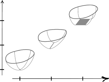
Figure 2: Energy landscape in supersymmetric theories: susy configurations minimize the energy for given topology, e.g. complex curves have minimal area, instantons have minimal Yang-Mills action etc. For fixed topology, they form finite-dimensional moduli spaces, of growing dimensions.

1.2 Boundaries and gluing

Whatever the exact flavor, a physical theory wants to have:

• a space-time manifold $M$, smooth or combinatorial, often with a metric, or some other fixed structures, and

• some degrees of freedom that are constrained on the boundary $\partial M$ and fluctuate in the bulk of $M$.

The integral over these fluctuations defines a map

$$\mathsf{Z}(M,\partial M):\,\,\textup{boundary conditions }\xrightarrow{}\textup{numbers}$$

which in a theory with local interactions has to satisfy the following basic gluing property.

Let $S\subset M$ a hypersurface that avoids $\partial M$ and let $M_{1}$ and $M_{2}$ be the manifolds with boundary into which $S$ cuts $M$. In the functional integral, we can first fix the degrees of freedom along $S$ and then integrate over them. In a local theory, the fluctuations in $M_{1}$ and $M_{2}$ will be independent once they are fixed along $S$, giving

$$\mathsf{Z}(M,\partial M)=\int\mathsf{Z}(M_{1},\partial_{1}M\sqcup S)\,\mathsf{Z}(M_{2},\partial_{2}M\sqcup S)\,,$$ (1)

where $\partial_{i}M=\partial M\cap M_{i}$ and the integral is over all possible boundary conditions on $S$. To be sure, the integral in (1) is at this point purely symbolical and is technically best expressed as a pairing between suitable functional spaces associated with $S$.

Figure 3: In a theory with local interactions, fluctuations on two sides of a hypersurface $S$ are independent once boundary conditions are imposed along $S$.

The equality (1) is very powerful as it:

• lets one compute $\mathsf{Z}(M,\partial M)$ by cutting $M$ into small pieces, and

• constraints these pieces thought the independence of (1) on the choice of $S$.

It gains real strength if $\mathsf{Z}(M,\partial M)$ factors through some large equivalence relation like e.g. orientation preserving diffeomorphisms, as this really reduces the number of standard pieces. This is the case for topological quantum field theories [AtTQFT, 43, WitTQFT], the Chern-Simons theory of real 3-folds being a very important example.

1.3 Boundaries and gluing in algebraic geometry

1.3.1

We want something like the setup of Section 1.2 but for a smooth quasiprojective algebraic variety $X$ in place of a smooth real manifold $M$. We don’t loose or gain anything by taking coefficients in $\mathbb{C}$, and for complex $X$ the story can, in principle, be squeezed into the above real mold. However, I think the cognitive efficiency is maximized here at the level of analogies, not precise matches.

We will allow noncompact $X$ as longs as objects that we want to count (basically, complete cuves in $X$) form moduli spaces that are either proper or proper over some other space of interest. Further, equivariant counts with respect to some torus

$$\mathsf{T}\subset\operatorname{Aut}(X)$$

may be defined as long as $\mathsf{T}$-invariant curves have compact moduli.

1.3.2

In place of $\partial M$, we will take an arbitrary smooth divisor $D\subset X$. This is a very inclusive interpretation of an algebraic analog of $\partial M$, people often insist on calling an effective anticanonical divisor the boundary of $X$, see in particular [KhRos]. While this is certainly a very important special case, there is no reason for us not to look beyond it.

1.3.3

The analog of topological invariance will be the invariance of $\mathsf{Z}(X,D)$ with respect to deformations of the pair $(X,D)$. This deformation will have to be equivariant for $\mathsf{T}$-equivariant counts.

1.3.4

The analog of (1) will hold when $X$ degenerates into a union of $X_{1}$ and $X_{2}$ as follows

(2)

where $\mathbb{A}^{1}$ is the base of the deformation, the total space $\widetilde{X}$ is smooth, and the special fiber is the transverse union of two components along a smooth divisor $D$. A one-dimensional example of this is

$$\{xy=1\}\subset\{xy=t\}\supset\{xy=0\}\,,$$

where $t$ gives the map to $\mathbb{A}^{1}$, and this is what it looks like in general in directions transverse to $D$. In (2), we assume that $D$ is disjoint from any other divisors chosen in $X$, in parallel to the $S\cap\partial M=\varnothing$ assumption in Section 1.2.

Figure 4: The algebraic analog of cutting a manifold along a hypersurface is a degeneration of $X$ to a transverse union of $X_{1}$ and $X_{2}$ along a divisor.

1.3.5

An important example of such degeneration is

(3)

which can be considered for any smooth divisor $D\subset X$. Here

$$\mathbb{B}=\mathbb{P}(N_{X/D}\oplus\mathscr{O}_{D})$$ (4)

is $\mathbb{P}^{1}$-bundle over $D$ associated to the rank 2 vector bundle $N_{X/D}\oplus\mathscr{O}_{D}$, where $N_{X/D}$ is the normal bundle to $D$ in $X$.

The manifold (4) is an algebraic analog of

$$\begin{matrix}\textup{tubular neighborhood}\\ \textup{of $\partial M$ in $M$}\end{matrix}\quad\cong\quad\partial M\times[0,1]$$

and similarly to this it has two boundary pieces isomorphic to $D$ namely

$$D_{0}=\mathbb{P}(N_{X/D})\subset\mathbb{B}\supset\mathbb{P}(\mathscr{O})=D_{\infty}\,.$$ (5)

Practitioners of DT theory like to give affectionate nicknames to the objects of the study, but there is little or no consistency in this. We will call $\mathbb{B}$ bubble in these notes, this is not a name that is in common use.

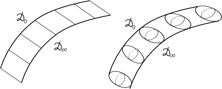
Figure 5: An algebraic geometer’s and a complex geometer’s impression of the bubble $\mathbb{B}$. This is the algebraic analog of a tubular neighborhood of $\partial M$ in $M$.

1.3.6

There is a natural equivalence relation induced by (2), namely

$$[X]=[X_{1}]+[X_{2}]-[\mathbb{B}]$$ (6)

where

$$\mathbb{B}=\mathbb{P}(N_{X_{1}/D}\oplus\mathscr{O}_{D})=\mathbb{P}(N_{X_{2}/D}\oplus\mathscr{O}_{D})\,.$$

The two formulas for $\mathbb{B}$ are equivalent because $N_{X_{1}/D}\cong N_{X_{2}/D}^{\vee}$.

A very powerful result of Levine and Pandharipande [50] is that the equivalence relation (6) generates all relations of the algebraic cobordism, and, in particular, any projective $X$ may be linked to a product of projective spaces by a sequence of such degenerations. While (6) by itself does not reduce the DT theory to that of

$$X\in\left\{\mathbb{P}^{3},\mathbb{P}^{2}\times\mathbb{P}^{1},\left(\mathbb{P}^{1}\right)^{3}\right\}\,,$$ (7)

it limits the number of standard pieces from which all other geometries may be assembled.

1.3.7

In the presence of a group action, e.g. for the toric varieties in (7), equivariant localization gives a way to cut $X$ further into really noncompact pieces, and this will be very important for us in Section 6.

1.4 What fluctuates ?

1.4.1

Donaldson-Thomas theory is for algebraic threefolds

$$\dim X=3$$

and in the original vision of [DonTh] the fluctuating degrees of freedom are given by a coherent sheaf $\mathscr{F}$ on $X$, or maybe a complex thereof. For a second, one can imagine that $\mathscr{F}$ is an algebraic vector bundle on $X$, although the main role in what follows will be played by sheaves in a sense diametrically opposite to vector bundles.

The inspiration for this came, among other things, from the Chern-Simons theory of real 3-folds, and also from Donaldson’s theory for real 4-folds. The latter involves integration over moduli spaces of instantons, that is, connections with antiselfdual curvature. For a Kähler surfaces $S$ viewed as a real 4-fold, a theorem of Donaldson [DonKr] identifies instantons with stable holomorphic vector bundles on $S$, and so one is really integrating over those. On the other hand, holomorphic bundles on a complex 3-fold are critical points of the holomorphic Chern-Simons functional (41), which links DT and CS theories.

A most superficial review of these points will be attempted in Section 3 below.

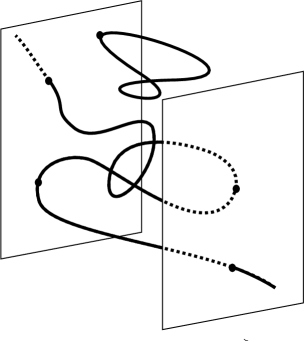
Figure 6: For us, the DT theory is the theory of fluctuating algebraic curves in $X$, constrained by how they meet fixed divisors $D\subset X$.

1.4.2

In these notes, however, we won’t see any vector bundles on $X$, and instead we will be looking at sheaves that look like the first or, equivalently, the last term in an exact sequence of the form

(8)

where $C\subset X$ is a curve, or more precisely, a $1$-dimensional projective subscheme. Of course, in general a subscheme is precisely defined from a subsheaf or a quotient of $\mathscr{O}_{X}$ as in (8), but at the first encounter it may be useful to think of a nice smooth curve which is embedded in $X$ and then allowed to move.

The moduli space for complexes (8) is the good old Hilbert scheme $\operatorname{Hilb}(X,\textup{curves})$ of Grothendieck, see e.g. [FDA, Koll]. The Hilbert scheme can be defined for $C$ and $X$ of arbitrary dimension, but there is something new and different in how one integrates over it, and other moduli of sheaves, for $\dim X=3$.

1.4.3

The Hilbert scheme splits into components $\operatorname{Hilb}(X,[C],\chi)$ according to the degree and the arithmetic genus of $C$

$$([C],\chi(\mathscr{O}_{C}))\in H_{2}(X,\mathbb{Z})\oplus H_{0}(X,\mathbb{Z})\,,$$

and a DT partition function is defined as a generating function over these discrete invariants. This means that

$$\mathsf{Z}(X,D)=\sum_{(d,n)\in H_{2}(X,\mathbb{Z})\oplus H_{0}(X,\mathbb{Z})}Q^{d}\,(-z)^{n}\,\,\,\int_{\operatorname{Hilb}(X,d,n)}\dots$$ (9)

where $z$ and $Q$ are new variables serving to keep track of the degree and genus, and $Q^{d}$ is a multiindex. The minus sign in $(-z)^{n}$ in (9) is introduced to save on signs in many other places.

1.4.4

There is a number of good reasons to focus on curves within the universe of coherent sheaves, among them:

• the theory can be defined for very general $X$, in particular, without any assumptions on the canonical class $\mathscr{K}_{X}$,

• the corresponding counts have a multitude of deep connections to other enumerative theories as well as other fields of mathematics such as representation theory,

• I expect, and I imagine that this expectation is shared by many, that the curve counts are fundamental and other sheaf counting problems may be reduced to them in some effective way.

Certainly, the last part is only a vague expectation and useless unless made precise. As a transition from curves to higher rank sheaves one can study theories where e.g. more than one section of $\mathscr{F}$ in (13) are considered, see e.g. [Bakk].

1.5 Integration

We need to explain what is meant by the integral in (9). Certainly cutting down the functional integral to an integral over a finite-dimensional space constitutes major progress, but the truth is that $\operatorname{Hilb}(X,d,n)$ has an unknown number of irreducible components of unknown dimensions, so it is not clear how one could integrate anything over its fundamental class. Human incompetence in basic geometry of Hilbert schemes starts with the simplest possible case $\operatorname{Hilb}(\mathbb{A}^{3},0,n)$ of points in a linear space. The dimension of this scheme is unknown except for small $n$.

While describing e.g. the irreducible components of $\operatorname{Hilb}(\mathbb{A}^{3},0,n)$ is an interesting geometric challenge, this is not the direction in which the development of the DT theory goes. Going back all the way to Section 1.1, the finite-dimensional integral over

$$\mathscr{M}=\textup{moduli of susy configurations}$$

is really a residue of a certain infinite-dimensional integral. The space $\mathscr{M}$ is cut out by certain equation, typically nonlinear PDEs like the equation $\bar{\partial}^{2}=0$ for a connection on a holomorphic vector bundle. When these equations are transverse, $\mathscr{M}$ is a finite-dimensional manifold and we may expect the functional integral to localize to the Lebesgue measure on $\mathscr{M}$.

However, in real life, equations are seldom transverse, which is how one is getting very singular varieties of unknown dimension whose fundamental cycle has nothing to do with the original integral. The original integral localizes to a certain virtual fundamental cycle

$$\left[\mathscr{M}\right]_{\textup{vir}}\in H_{2\operatorname{vir\,dim}}\left(\mathscr{M}\right)\,,$$ (10)

where the virtual, or expected, dimension may be computed from counting the degrees of freedom and is typically some Riemann-Roch computation. For example

$$\operatorname{vir\,dim}\operatorname{Hilb}(X,d,n)=d\cdot c_{1}(X)\,.$$

Analytically, the virtual cycle may be constructed by a very small perturbation of the equations that puts them into general position. For what we have in mind, this is both too inexplicit and will certainly break the symmetries of the problem that are so important for equivariant counts.

It is much better to treat the problem as an excess intersection problem in algebraic geometry and construct the cycle using certain vector bundles on $\mathscr{M}$ that describe the deformations and equations at $\mathscr{M}$. This data is called an obstruction theory and the construction of virtual cycles from it was given in the fundamental paper of Behrend and Fantechi [12]. The obstruction theory for DT problems was constructed by R. Thomas in [ThCass], this is the technical starting point of DT theory. We will get a feeling how this works below.

With this, (9) should be made more precise as follows

$$\mathsf{Z}(X,D)=\sum_{(d,n)\in H_{2}(X,\mathbb{Z})\oplus H_{0}(X,\mathbb{Z})}Q^{d}\,(-z)^{n}\,\,\,\int_{\left[\operatorname{Hilb}(X,d,n)\right]_{\textup{vir}}}\dots$$ (11)

where dots stand for cohomology classes that come from the boundary conditions, as will be discussed in a moment. For now we note that beyond the virtual fundamental cycle, the DT moduli spaces $\mathscr{M}$ have a virtual $\hat{A}$-genus

$$\widehat{\mathscr{O}}_{\textup{vir}}\in K(\mathscr{M})$$

with which one can define a K-theoretic analog of (11)

$$\mathsf{Z}(X,D)_{\textup{K-theory}}=\sum_{(d,n)\in H_{2}(X,\mathbb{Z})\oplus H_{0}(X,\mathbb{Z})}Q^{d}\,(-z)^{n}\,\,\,\chi\left(\widehat{\mathscr{O}}_{\operatorname{Hilb}(X,d,n),\textup{vir}}\otimes\dots\right)$$ (12)

defined in the $\operatorname{Aut}(X)$-equivariant K-theory.

1.6 PT theory

1.6.1

Abstract DT theory may be described as counting stable objects in categories that are akin (that is, have similar properties of ${\operatorname{Ext}}^{\raisebox{1.42262pt}{$\scriptscriptstyle\bullet$}}$-groups) to coherent sheaves on a smooth threefold. These notes are not the place to go into a discussion of stability and its variations, which is a deep and technical notion, see e.g. [Br1, 19, 20, KS]. But one example of how the change of stability can drastically simplify moduli spaces must be discussed. This is the moduli space of stable pairs, a simpler cousin of the Hilbert schemes of curves, first used in the enumerative context by Pandharipande and Thomas [PT1, PT2].

1.6.2

Recall that a point in the Hilbert scheme of curves corresponds to a coherent sheaf $\mathscr{F}=\mathscr{O}_{C}$ that is a $1$-dimensional quotient

$$\mathscr{O}_{X}\xrightarrow{\,\,s\,\,}\mathscr{F}\to 0$$ (13)

of $\mathscr{O}_{X}$. In this arrangement, the map $s$ is very good (surjection) but the sheaf $\mathscr{F}$ can be quite bad. The problems with $\mathscr{F}$ start already for the Hilbert schemes of points, that is, for $\dim\mathscr{F}=0$, and pollute all curve counts of positive degree. One can’t help feeling that there should a way to disentangle the contributions of points and curves and, to a large extent, this is exactly what PT theory achieves.

In PT theory, one ask less of $s$ and more of $\mathscr{F}$. What we want from $\mathscr{F}$ is to be a pure 1-dimensional sheaf, that is, to have no 0-dimensional subsheaves. For instance, if $\dim\operatorname{supp}\mathscr{F}=0$ then we must have $\mathscr{F}=0$. What we are willing to allow of $s$ is that

$$\dim\operatorname{Coker}s=0$$

instead of $\operatorname{Coker}s=0$.

For example, if the support of $\mathscr{F}$ is a reduced smooth curve $C$ then the only stable pairs are of the form

(14)

where $\{p_{i}\}\subset C$ is an unordered collection of points and the other two maps in (14) are the natural ones. In other words, the fiber of the PT moduli spaces over the point

$$[C]\in\operatorname{Chow}(X)=\{\textup{effective $1$-cycles in $X$}\}$$

corresponding to a smooth curve $C\subset X$ is ${\mathsf{S}}^{\raisebox{1.42262pt}{$\scriptscriptstyle\bullet$}}(C)=\bigsqcup_{n}\mathsf{S}^{n}C$. This is infinitely simpler than the fiber of the Hilbert schemes of curves.

1.6.3

Obviously, PT counts cannot agree with the Hilbert scheme counts because they do not agree already in degree 0. It is, however, conjectured that they agree once one takes this into account and divides out the contribution of points from the generating function, that is

$$\mathsf{Z}_{\textup{PT}}(Q,z)=\mathsf{Z}_{\textup{Hilb}}(Q,z)\bigg{/}\mathsf{Z}_{\textup{Hilb}}(0,z)\,.$$ (15)

The denominator in (15) was computed explicitly for an arbitrary 3-fold for the needs of the GW/DT correspondence. This will be discussed in Section 5.4.

For toric 3-folds, the equality (15) comes out of the whole machine that computes their DT counts [57]. For Calabi-Yau 3-folds, Y. Toda gave a proof [Toda1, Toda2] that analyses wall-crossing connecting the Hilbert scheme stability condition to the stability condition for stable pairs. Wall-crossing techniques have not been really explored outside the world of Calabi-Yau varieties.

1.7 Actual counts

Actual DT counts are very complex. While they are defined for a general smooth divisor $D$ in a general smooth threefold $X$, it is not even clear if there is a universal language in which the answers can be stated, starting with the case $D=\varnothing$.

We understand the answers explicitly for very special $X$, like the toric varieties with $D=\varnothing$ or certain fibrations with $D=\bigcup\textup{\sl Fibers}$ that will be discussed in Sections 6 and 7. Already these are very rich and seem to require, more or less, all of the mathematics that falls into the author’s area of expertise for their understanding.

I view this is a great advantage of the DT theory: there are certainly whole galaxies of open problems in it of all possible flavors — from foundational to combinatorial. One of my goals in these notes is to help potential explorers of these galaxies to get a sense of what awaits them there.

2 Boundary conditions and gluing

Now we put the boundary conditions in (11), that is, we constrain the fluctuating curve $C$ by how it intersects our fixed divisor $D$.

2.1 Intersection with the boundary

2.1.1

Algebraically, functions on $C\cap D$ are the functions on $C$ taken modulo the equation of $D$, that is, they are the cokernel in

$$\mathscr{O}_{C}\xrightarrow{\textup{$\times$ equation of D }}\mathscr{O}_{C}\to\mathscr{O}_{C\cap D}\to 0\,.$$ (16)

There is an open locus

$$\operatorname{Hilb}(X,d,n)^{\perp}\subset\operatorname{Hilb}(X,d,n)$$ (17)

where the first arrow in (16) is injective. This is the correct transversality condition on $C\cap D$ for us. For transverse curves (17), we have a well-defined map

$$\cdot\,\cap D:\quad\mathscr{O}_{C}\mapsto\mathscr{O}_{C\cap D}\in\operatorname{Hilb}(D,d\cdot[D])\,,$$ (18)

to the Hilbert scheme of $d\cdot[D]$ points in $D$.

2.1.2

Contrary to the 3-fold case, Hilbert schemes of points in surfaces are exceptionally nice algebraic varieties. In particular, they are smooth and connected of dimension

$$\dim\operatorname{Hilb}(D,k)=2k\,.$$

An introduction to their geometry may be found in [Lehn, NakL]. As lots of things in DT theory are built on the geometry of $\operatorname{Hilb}(D,k)$, we will be often coming back to it in these notes.

2.1.3

Imposing boundary conditions means integrating along the fibers of (18) or, equivalently, pulling back cohomology classes from $\operatorname{Hilb}(D)$ via (18). Neither is well-defined because (17) is open, meaning some further details need to be filled in here.

There are, in fact, at least 3 ways to do it, as will be discussed presently. The conventions on what to call these flavors of boundary condition vary. We will call them nonsingular, relative, and descendent, respectively. While they all express the same general geometric idea of $C$ meeting $D$ in a particular way, an actual geometric translation between them is not trivial and plays an important role in the development of the theory, see below.

2.1.4

Once the technical details are filled in, the special structures in the (co)homology of the Hilbert scheme serve to organize the DT data in a very nice way. In particular, one can interpret (11) as

$$\mathsf{Z}(X,D)=(\cdot\cap D)_{*}\left(\sum Q^{d}\,(-z)^{n}\,\left[\operatorname{Hilb}(X,d,n)\right]_{\textup{vir}}\right)\in{H}_{\raisebox{1.42262pt}{$\scriptscriptstyle\bullet$}}(\operatorname{Hilb}(D))[[Q,z]]\,,$$ (19)

where

$${H}_{\raisebox{1.42262pt}{$\scriptscriptstyle\bullet$}}(\operatorname{Hilb}(D))=\bigoplus_{k}{H}_{\raisebox{1.42262pt}{$\scriptscriptstyle\bullet$}}(\operatorname{Hilb}(D),k)\cong\mathsf{Fock}\left({H}_{\raisebox{1.42262pt}{$\scriptscriptstyle\bullet$}}(D)\right)\,.$$ (20)

The important and powerful identification of (co)homology with Fock space modelled on the (co)homology of the surface $D$ itself is a classical result of [NakHart].

2.2 Different flavors of boundary conditions

2.2.1 Nonsingular bc

The $\mathsf{T}$-fixed locus

$$\left(\operatorname{Hilb}(X,d,n)^{\perp}\right)^{\mathsf{T}}\subset\operatorname{Hilb}(X,d,n)^{\perp}$$

may be compact for some torus $\mathsf{T}\subset\operatorname{Aut}(X,D)$, in which case the boundary conditions may be imposed for equivariant counts in localized equivariant cohomology without further geometric constructions.

For example, the bubble (4) has a fiberwise $\mathbb{C}^{\times}$ action that fixes both divisors in (5) and can be used to impose the nonsingular boundary conditions at either of them. As an exercise, one should check that imposing nonsingular conditions at both $D_{0}$ and $D_{\infty}$ gives trivial DT counts, in the sense that

$$\left(\operatorname{Hilb}(\mathbb{B},d,n)^{\perp D_{0}\cup D_{\infty}}\right)^{\mathbb{C}^{\times}}\cong\begin{cases}\operatorname{Hilb}(D,k)\,,&(d,n)=k[\textup{fiber $\mathbb{B}\to D$}]\,,\\ \varnothing\,,&\textup{otherwise}\,,\end{cases}$$

and that in the former case the virtual cycle pushes forward to

$$\textup{diagonal}\subset\operatorname{Hilb}(D_{0},k)\times\operatorname{Hilb}(D_{\infty},k)\,.$$

2.2.2 Relative bc

There is a resolution of the map (18), that is, a diagram of the form

(21)

in which the new map to $\operatorname{Hilb}(D,d\cdot[D])$ is proper. Here $\operatorname{Hilb}(X/D,d,n)$ is the Hilbert scheme of curves relative the divisor $D$. It is constructed using J. Li’s theory of expanded degenerations [Li1]. It allows $X$ to sprout off new components as in (3) as many times as needed to keep $C$ transverse to $D$. A more complicated instance of the same general phenomenon is illustrated in Figure 7.

Note that in the central fiber of (3) the proper transform of the divisor $D$ escapes to the new component and becomes the divisor $D_{\infty}$ in (5). This is the new divisor $D$ with which we intersect the subscheme $C$.

With relative boundary conditions, we integrate over $\operatorname{Hilb}(X/D,d,n)$ in (11) and (19).

2.2.3 Descendent bc

Instead of trying to pull back cohomology classes from $\operatorname{Hilb}(D,d\cdot[D])$, we can construct the corresponding classes directly on $\operatorname{Hilb}(X,d,n)$ as follows. It is well known that the ${H}^{\raisebox{1.42262pt}{$\scriptscriptstyle\bullet$}}(\operatorname{Hilb}(D))$ is generated by the Künneth components of the Chern classes of $\mathscr{O}_{\mathscr{Z}}$ where

$$\mathscr{Z}\subset\operatorname{Hilb}(D)\times D$$

is the universal subscheme. We have a well-defined class

$$\mathscr{O}_{C}\otimes_{\textup{K-theory}}\mathscr{O}_{D}\in K^{\circ}(\operatorname{Hilb}(X)\times D)$$ (22)

where $K^{\circ}$ is the K-theory of locally free sheaves. It has Chern classes, the Künneth components of which can be inserted in the integral over $\operatorname{Hilb}(X)$.

Note that these descendent cohomology classed do not factor through the relations in ${H}^{\raisebox{1.42262pt}{$\scriptscriptstyle\bullet$}}(\operatorname{Hilb}(D))$. In other words, they are really not pulled back via some map like (18). As we will see in a minute, they can be translated into the relative conditions, but the coefficients in this translation are functions of $Q$ and $z$.

Also note that the structure sheaf of the universal curve

$$\mathscr{O}_{C}\in K^{\circ}(\operatorname{Hilb}(X,d,n)\times X)$$

also has Chern classes which we can similarly use to produce cohomology classes on $\operatorname{Hilb}(X,d,n)$. These can be also inserted into the integral in (11). Such insertions constrain the behaviour of $C$ in the bulk of $M$.

Note that the supply of descendent classes is, a priori, indexed not by the Fock space in (20) but by

$${H}^{\raisebox{1.42262pt}{$\scriptscriptstyle\bullet$}}_{GL(\infty)}(\textup{pt})\otimes{H}^{\raisebox{1.42262pt}{$\scriptscriptstyle\bullet$}}(D)\,\rightarrow\,\textup{descendent bc}\,,$$

that is, by arbitrary Chern classes colored by the cohomology of $D$. Chern classes colored by the cohomology of $X$ produce descendent bulk insertions.

2.3 Gluing

2.3.1

The following geometric considerations lead to the gluing formula in DT theory. Let $X$ break up in two pieces as in (2) and in Figure 4. This is as nice a degeneration of an algebraic variety as you will ever see and we want to have the nicest possible degeneration of the corresponding Hilbert schemes. The Hilbert scheme of the singular variety

$$X_{0}=X_{1}\cup_{D}X_{2}$$

while perfectly well-defined, is not nice, because if $C$ meets the $D=(X_{0})_{\textup{sing}}$ in a nontransverse way then this causes all sort of problem including a failure in the obstruction theory.

The solution, provided by J. Li’s theory of expanded degenerations [Li1] is to allow $X_{0}$ to open up accordions of the form

$$X_{0}[k]=X_{1}\cup_{D_{1}}\underbrace{\mathbb{B}\cup_{D_{2}}\dots\cup_{D_{k}}\mathbb{B}}_{\textup{$k$ times}}\cup_{D_{k+1}}X_{2}$$

where the bubble $\mathbb{B}=\mathbb{P}(N_{X_{1}/D}\oplus\mathscr{O}_{D})$ is already familiar from (4) and the discussion of relative boundary conditions. The divisors

$$D_{1}\cong D_{2}\cong\dots\cong D_{k+1}\cong D$$

are the copies of $D$ that appear together with the bubbles $\mathbb{B}$. The subschemes $C\subset X_{0}[k]$ what we allow have the form

$$C=C_{0}\cup C_{1}\cup\dots\cup C_{k}\cup C_{k+1}$$

where the components $\{C_{i}\}$ are transverse to the divisors $\{D_{i}\}$ and glue along them in the sense that

$$C_{i}\cap D_{i+1}=D_{i}\cap C_{i+1}\,.$$

A new bubble blows up any time transversality is in danger and the moduli spaces for different $k$ fit together into one orbifold

$$\operatorname{Hilb}(X_{0}[\cdot])=\bigcup_{k\geq 0}\operatorname{Hilb}(X_{0}[k])_{\textup{semistable}}\,\Big{/}(\mathbb{C}^{\times})^{k}$$

where $\mathbb{C}^{\times}$ acts on the $\mathbb{P}^{1}$-bundle fiberwise preserving the two divisors in (5). This is the right object to put as a central fiber in the family of degenerating Hilbert schemes.

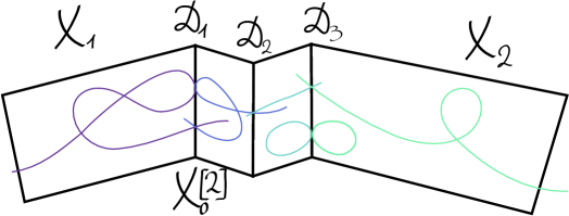
Figure 7: A curve in an expanded degeneration $X_{0}[n]$ is a collection of subschemes in each component that are transverse to the singular divisors and glue along them.

2.3.2

The gluing formula for DT proven in [52] is the combination of two statements. First

$$\int_{[\operatorname{Hilb}(X)]_{\textup{vir}}}\dots=\int_{[\operatorname{Hilb}(X_{0}[\cdot])]_{\textup{vir}}}\dots\,,$$ (23)

where the integrand is defined e.g. using boundary conditions away from $D$ or in any other way that makes sense as a cohomology class on the whole family of the Hilbert schemes. In other words, with the right definition, the deformation invariance of DT counts in the family (2) includes the central fiber.

2.3.3

The second part of the gluing formula says that the integral over the right-hand side in (23) can be computed in terms of DT counts in $X_{1}$ and $X_{2}$ relative the gluing divisor $D$. Concretely

$$Z(X)=\Big{(}Z(X_{1}/D),(-z)^{|\,\cdot\,|}\,Z(X_{2}/D)\Big{)}_{{H}_{\raisebox{1.42262pt}{$\scriptscriptstyle\bullet$}}(\operatorname{Hilb}(D))}$$ (24)

where we interpret $Z(X_{1}/D)$ as in (9) and $|\,\cdot\,|$ is the grading operator on the Fock space (20), it acts by $k$ on the $k$th term in the direct sum in (20). We write $Z(X_{1}/D)$ to stress the fact that relative conditions are imposed at the divisor $D$.

The extra weight $(-z)^{|\,\cdot\,|}$ in (24) is there because

$$\chi(\mathscr{O}_{C})=\chi(\mathscr{O}_{C_{1}})+\chi(\mathscr{O}_{C_{2}})-\chi(\mathscr{O}_{C_{1}\cap D})$$ (25)

if $C=C_{1}\cup_{C_{1}\cap D}C_{2}$ is a transverse union along the common intersection with $D$.

2.3.4

For K-theoretic counts, the first part (23) holds verbatim, but there is a correction to (24) discovered in [36]. It can be phrased by saying that the natural bilinear form used in (24) is deformed for K-theoretic counts in a way that depends on $Q$ and $z$. An introductory discussion of this issue may be found in Section 6.5 of [84].

2.4 Correspondence of boundary conditions

2.4.1

Let $D\subset X$ be a smooth divisor and imagine that some mystery boundary conditions are imposed on $D$ for curve counts in $X$. We can bubble off $D$ as in (3) and conclude from the gluing formula that

$$Z(X,\textup{mystery at $D$})=\\ \Big{(}Z(X/D_{0}),(-z)^{|\,\cdot\,|}\,Z(\mathbb{B},\textup{relative at $D_{0}$},\textup{mystery at $D_{\infty}$})\Big{)}_{{H}_{\raisebox{1.42262pt}{$\scriptscriptstyle\bullet$}}(\operatorname{Hilb}(D_{0}))}\,.$$ (26)

We conclude from (26) that DT counts in $\mathbb{B}$ with two flavors of the boundary conditions at $D_{0}$ and $D_{\infty}$ respectively precisely give the translation between different boundary conditions. Note this translation depends on $Q$ and $z$.

2.4.2

This is completely parallel to how one can translate between boundary conditions by imposing a full set of alternative boundary conditions on the other boundary of the tubular neighborhood in Figure 1.

While the correspondence given by (26) is a useful general statement, the concrete identification of $Z(\mathbb{B},D_{0},D_{\infty})$ may be a very challenging problem.

2.4.3

Recall that $\mathbb{B}$ has a fiberwise $\mathbb{C}^{\times}$-action that fixes $D_{0}$ and $D_{1}$. Equivariant localization with respect to this action gives

$$Z(\mathbb{B},\textup{$\mathsf{bc}_{0}$ at $D_{0}$},\textup{$\mathsf{bc}_{\infty}$ at $D_{\infty}$})=\\ \left(Z(\mathbb{B},\textup{$\mathsf{bc}_{0}$ at $D_{0}$},\textup{ns at $D_{\infty}$}),Z(\mathbb{B},\textup{ns at $D_{0}$},\textup{$\mathsf{bc}_{\infty}$ at $D_{\infty}$})\right)_{\textup{edge}}$$ (27)

where $\mathsf{bc}_{0}$ and $\mathsf{bc}_{\infty}$ denotes some arbitrary boundary conditions and the edge inner product on ${H}_{\raisebox{1.42262pt}{$\scriptscriptstyle\bullet$}}(\operatorname{Hilb}(D))$ is a new inner product that reflects the nontriviality of the fibration

$$\pi_{\mathbb{B}}:\mathbb{B}\to D\,.$$

It comes from the edge terms in localization formulas, see below, and is determined by the deformation theory of “constant” curves in $\mathbb{B}$, that is, ideal sheaves of the form

$$\pi^{*}_{\mathbb{B}}(\mathscr{I})\in\operatorname{Hilb}(\mathbb{B})\,,\quad\mathscr{I}\in\operatorname{Hilb}(D)\,.$$

Using (27) one can replace arbitrary boundary conditions by nonsingular ones in equivariant theory.

3 Before DT

3.1 Gromov-Witten theory

There is another curve-counting theory in algebraic geometry which can be defined for a smooth $X$ of arbitrary dimension. It traces its origins to the topological strings in the same way as DT theory descends from the study of supersymmetric gauge theories.

3.1.1 Moduli spaces

In GW theory, one integrates over the moduli spaces $\overline{\mathscr{M}}_{g,n}(X,d)$ of stable maps to $X$, where a point of $\overline{\mathscr{M}}_{g,n}(X,d)$ corresponds to the data

$$(C,p_{1},\dots,p_{n})\xrightarrow{\,\,f\,\,}X$$ (28)

in which

$$C \quad\textup{is an at worst nodal curve of genus $g$}\,,$$

$$p_{1},\dots,p_{n}\in C \quad\textup{are smooth distinct marked points of $C$}\,,$$

$$f \deg f:=f_{*}[C]=d$$ is a map of degree  .

Two maps are isomorphic if there exist a triangle

(29)

in which $\phi$ is an isomorphism of pointed curves. As a stability condition for the data (28), one requires the automorphism group of (28) to be finite.

The moduli spaces $\overline{\mathscr{M}}_{g,n}(X,d)$ have a canonical perfect obstruction theory of virtual dimension

$$\operatorname{vir\,dim}=(g-1)(3-\dim X)+c_{1}(X)\cdot d+n\,,$$ (30)

and the corresponding virtual fundamental classes in cohomology. In their K-theory, one has virtual structure sheaves but, in general, one does not have a good virtual $\hat{A}$-genus, in contrast to DT theories.

In GW theory one forms generating functions analogous to (11)

$$\mathsf{Z}_{\textup{GW}}(X;Q,u)=\sum_{(d,g)\in H_{2}(X,\mathbb{Z})\oplus\mathbb{Z}}Q^{d}\,u^{2g-2}\,\,\,\int_{\left[\overline{\mathscr{M}}_{g,n}(X,d)\right]_{\textup{vir}}}\dots\,,$$ (31)

the variable $u$ in which corresponds to the string coupling constant of topological strings.

An excellent introduction to stable maps and GW theory may be found in [mirror_book].

3.1.2 Relative GW theory

A stable map is transverse to a divisor $D$ if the set

$$f^{-1}(D)=\{b_{i}\}$$

is finite and disjoint from nodes and marked points in (28). Counting multiplicity, we have

$$f^{*}D=\sum\mu_{i}\,[b_{i}]\,,\quad\mu_{i}\in\mathbb{N}=\{1,2,\dots\}\,,$$

and it is convenient to add the points $\{b_{i}\}$ and the multiplicities $\{\mu_{i}\}$ to the data in (28) to get a new moduli space with morphisms

$$\overline{\mathscr{M}}_{g,n,\mu}(X/D,d)\owns f\mapsto f(b_{i})\in D$$ (32)

that take a map $f$ to its $i$th point of tangency with $D$. Expanded degenerations provide a natural compactification of this relative moduli space.

As boundary conditions we pull back classes in ${H}^{\raisebox{1.42262pt}{$\scriptscriptstyle\bullet$}}(D)$ via (32). These are additionally colored by the integers $\mu_{i}$ and this color may be recorded by a monomial $t^{\mu_{i}}$. This gives

relative bc $$={\mathsf{S}}^{\raisebox{1.42262pt}{$\scriptscriptstyle\bullet$}}\left({H}^{\raisebox{1.42262pt}{$\scriptscriptstyle\bullet$}}(D)\otimes t\mathbb{Q}[[t]]\right)$$ (33)

$$=\mathsf{Fock}({H}^{\raisebox{1.42262pt}{$\scriptscriptstyle\bullet$}}(D))\,,$$

where the symmetric algebra takes into account the sign rules, that is, is the symmetric algebra in the category of $(\mathbb{Z}/2)$-graded vector spaces.

The parallel with the discussion of Section 2.1.4 is not coincidental.

3.1.3 Different dimensions

Since the GW counts are defined for $X$ of arbitrary dimension, it is natural to ask how the counts are affected by simple changes of geometry like going from $X$ to $X\times\mathbb{A}^{1}$.

Despite the obvious noncompactness, $\mathbb{C}^{\times}$-equivariant GW counts in $X\times\mathbb{A}^{1}$ are well-defined for the natural $\mathbb{C}^{\times}$ action on $\mathbb{A}^{1}$. Denoting by $t$ the weight of this action, the difference $\delta$ in the obstruction theory between maps to $X\times\mathbb{A}^{1}$ and maps to $X$ is

$$\delta\left(\operatorname{Def}-\operatorname{Obs}\right)={H}^{\raisebox{1.42262pt}{$\scriptscriptstyle\bullet$}}(C,f^{*}(T\mathbb{A}^{1}))=\\ ={H}^{\raisebox{1.42262pt}{$\scriptscriptstyle\bullet$}}(C,t\otimes\mathscr{O}_{C})=t-t\otimes H^{1}(\mathscr{O}_{C})=t-t\otimes H^{0}(\omega_{C})^{\vee}\,.$$ (34)

The rank $g$ bundle $H^{0}(\omega_{C})$ is known as the Hodge bundle over the moduli spaces of curves. Its fiber over a smooth curve $C$ is formed by the holomorphic differentials on $C$. Note that the rank in (34) is $1-g$ in agreement with the virtual dimension formula (30).

This difference in obstruction theories means the insertion of

$$t^{-1}\textup{Euler}(t\otimes H^{0}(\omega_{C})^{\vee})=\sum_{k}(-1)^{k}t^{g-k-1}c_{k}(\textup{Hodge})$$

in the integral over $\overline{\mathscr{M}}_{g,n}(X)$. Integrals with Chern classes of the Hodge bundle are known as the Hodge integrals. We see that such insertions are equivalent to extra factors of $\mathbb{A}^{1}$ in the target of stable maps. In particular, the equivariant GW theory of a linear space is the theory of Hodge of integrals over the the Deligne-Mumford moduli spaces of stable curves.

Note that Hodge integrals are suppressed in the $t\to\infty$ limit. More generally, the GW theory of $X^{\mathsf{T}}$ may be recovered from GW theory of $X$ if we send all equivariant variables to infinity.

3.1.4 Periodicity

If we are willing to increase dimension by 2 then there is a cleaner relation that does not require taking limits in $t$. The following vanishing of Chern classes

$$\textup{Euler}\left(t\otimes\left(\textup{Hodge}\oplus\textup{Hodge}^{\vee}\right)\right)=t^{2g}$$ (35)

was noticed by Mumford and for smooth curves may be explained by the existence of the natural flat connection on the rank $2g$ bundle

$$H^{1}(C,\mathbb{C})=H^{1}(\mathscr{O})\oplus H^{0}(\Omega^{1}_{C})\,,$$

see [FP] for a modern discussion. It follows that

$$\mathsf{Z}_{\textup{GW}}(X\times\mathbb{A}^{2}_{(t,-t)};Q,u)=\mathsf{Z}_{\textup{GW}}(X;Q,itu)$$ (36)

where $t\in\operatorname{Lie}\mathbb{C}^{\times}$ acts on $\mathbb{A}^{2}_{(t,-t)}$ by $\begin{pmatrix}t\\ &-t\end{pmatrix}$.

3.1.5 Critical dimension

It is clear from (30) that the case

$$\dim X=3$$

is very special in GW theory. Virtual dimension grow/diminish with genus for $\dim X\gtrless 3$ and are independent of the genus for $\dim X=3$. Precisely for threefolds, one can have interesting generating functions over all genera with the same insertions, in particular, with the same boundary conditions.

As discussed above, equivariant GW theory of threefolds also contains the GW theory of targets of smaller dimension.

3.1.6 Compare and contrast

There is a precise and very nontrivial comparison between the GW theory in its critical dimension and the DT theory. This comparison has been one of the guiding stars for the development of the DT theory and will be discussed properly below.

Since these lectures are about DT theory, naturally, we will be stressing those aspects of the DT theory in which it compares favorably to GW theory. These include, for instance, the ease of “boxcounting” localization computations, a feature much appreciated by practitioners and students alike. More fundamentally, DT theory is much better suited for going beyond the computations in cohomology as its partition functions may be computed not only in K-theory but, in special circumstances, in even more refined enumerative theories.

But in fairness to GW theory, one should not forget to stress its great scope and flexibility. Not only is it defined for smooth algebraic varieties of any dimension, it can also count pseudoholomophic surfaces in real symplectic manifolds $M$, and those can even have boundaries ending on Lagrangian subvarieties of $M$. Already the counts of pseudoholomophic disks in such situations form a structure of stunning richness captured by Fukaya categories of different flavors. These constrain the counts of holomorphic curves and, one day, may help with the actual computations.

3.2 Chern-Simons theory

3.2.1

In Chern-Simons theory, the space-time is an oriented 3-manifold $M$ and one integrates over gauge-equivalence classes of connections $A$ on a $G$-bundle, where $G$ is a simple Lie group such as $G=SU(n)$. The integrand is $\exp(2\pi ik\,\mathsf{CS}(A))$ where

$$\mathsf{CS}(A)=\frac{1}{8\pi^{2}}\int_{M}\operatorname{tr}\left(A\wedge dA+\tfrac{2}{3}\,A\wedge A\wedge A\right)\,.$$ (37)

The critical points of which are flat connections:

$$\nabla\mathsf{CS}=0\quad\Leftrightarrow\quad F_{A}=0\,.$$ (38)

More precisely, (37) picks up an integer, the degree of the map $M\to G$ under a general gauge tranformation, whence the quantization of the level $k\in\mathbb{Z}$, which is a very important feature of the theory. This does not affect (38), nor does it affect the fact that flat connections make the dominant contribution to the integral in the semiclassical $k\to\infty$ limit.

We have

$$\left\{\textup{flat $A$}\right\}\Big{/}\textup{gauge}=\operatorname{Hom}(\pi_{1}(M)\to G)/G\,,$$ (39)

where the $G$-action on the right is by conjugation. As a critical locus, (39) has expected dimension zero, which is also confirmed by the deformation theory of flat connections. Correctly counting points of (39) represents various generalization of the Casson invariant, see [Taubes] for a classical treatment.

3.2.2

Donaldson-Thomas theory originated [DonTh] from the following precise analog of (37) for complex Calabi-Yau threefolds $X$. Flat connections are now replaced by $\bar{\partial}$-operators

$$\bar{\partial}_{A}=\bar{\partial}+A\,,\quad A\in\{\textup{(0,1)-forms}\}\otimes\operatorname{End}(\mathscr{E})\,,$$

that give the structure of a holomorphic bundle to a $C^{\infty}$-bundle $\mathscr{E}$ over $X$, provided they satisfy

$$\bar{\partial}_{A}^{2}=0\,.$$ (40)

The holomorphic Chern-Simons functional

$$\mathsf{CS}_{\textup{holo}}(A)=\int_{M}\operatorname{tr}\left(A\wedge\bar{\partial}A+\tfrac{2}{3}\,A\wedge A\wedge A\right)\wedge\Omega^{3}\,,$$ (41)

where $\Omega^{3}$ is the holomorphic 3-form on $X$, the normalization of which is of no importance here, similarly satisfies

$$\nabla\mathsf{CS}_{\textup{holo}}=0\quad\Leftrightarrow\quad\bar{\partial}_{A}^{2}=0\,.$$ (42)

As reflected in the title of [ThCass], the DT theory was seen originally as an analog of the Casson invariant in algebraic or complex geometry. As the scope of DT theory broadened, there are now both conceptual and technical advantages to seeing Casson invariants as a particular instance of DT-like counts.

3.2.3

Natural observables in CS theory are Wilson lines, that is, holonomies of $A$ along a curve $K\subset M$, which is a link in $M$, for instance a knot, whence the notation. A very influential set of ideas that originated with Witten [WittCS], equates those with the counts of open pseudoholomorphic surfaces

$$C\subset T^{*}M$$

ending on the conormal $L_{K}=T^{\perp}K\subset T^{*}M$ to the link $K$, which is a Lagrangian submanifold of $T^{*}M$. In many cases, these should further correspond to counts of complete $C$ in some associated algebraic varieties, see [GopVafa, OogVafa]. This line of inquiry was the principal inspiration for the topological vertex conjecture of [AKMV], see Section 6.3.4, which in turn ignited a lot of research in DT theory.

3.2.4

There is another very important inspiration that DT theory draws from CS theory and it is about the role of representation theory in geometry.

The action (37) does not involve a metric on $M$ which makes CS theory topological. It can thus be understood in terms of a small number of standard pieces and representation theory of affine Lie algebras and/or quantum groups associated to $G$ is fundamental for describing those, see e.g. [BakKir, Kohno].

In DT theory, one similarly desires to describe the standard pieces of the theory in terms of (geometric) representation theory, and we will get a sense how this works in Section 7, see [84, 85] for more.

3.3 Nekrasov theory

While Nekrasov’s theory may be classified as an equivariant version of Donaldson’s invariants of smooth 4-manifolds, its distinctive goals and technical tools had a very significant influence on the development of the DT theory.

3.3.1

Let $A$ be a connection on a trivial rank $r>1$ bundle over $M=\mathbb{R}^{4}$, which is the Euclidean version of the Minkowski space-time of our everyday experience. If finite, the Yang-Mills energy

$$\mathsf{YM}(A)=\int_{M}\|F_{\mathbb{A}}\|^{2}$$

of $A$ is bounded below by a topological invariant

$$\int_{M}\operatorname{tr}F\wedge F=8\pi^{2}c_{2}(F)\leq\mathsf{YM}(A)$$ (43)

with an equality if $A$ is an instanton, also known as an anti-self-dual connection. The integral (43) agrees with the topologically defined Chern class $c_{2}$ for an extension of $A$ to $S^{4}\supset\mathbb{R}^{4}$ as in [Uhl]. Modulo gauge transformations that are trivial at $\infty\in S^{4}$, instantons are parametrized by a smooth manifold $\mathscr{M}$ of real dimension $4rc_{2}$. The integrals over $\mathscr{M}$ may be interpreted as (very!) approximate answers in Euclidean Yang-Mills theory or as exact answers with enough supersymmetry and twists. This is the physical interpretation of Donaldson’s theory of integration over a certain compactification of $\mathscr{M}$ for general $4$-manifold, see [WitTQFT, WittenDon].

3.3.2

By a theorem of Donaldson [DonGIT], $\mathscr{M}$ is also the moduli spaces of holomorphic bundles on $X=\mathbb{C}^{2}\cong\mathbb{R}^{4}$ that are trivial at infinity in the following sense. Pick an embedding into a projective surface

$$X\subset\overline{X},\quad\textup{e.g.}\quad\overline{X}=\mathbb{P}^{2}$$

and consider holomorphic bundles on $\overline{X}$ together with a trivialization

$$\phi:\mathscr{F}|_{D}\xrightarrow{\,\sim\,}\mathscr{O}_{D}^{\oplus r}\,,\quad D=\overline{X}\setminus X\,,$$

known as a framing of $\mathscr{F}$. The group $GL(r)\cong\operatorname{Aut}\mathscr{O}_{D}^{\oplus r}$ acts on $\phi$, and this is the same action as the action of constant gauge transformations on instantons.

In one sentence, Nekrasov theory [NekInst] may be described as $G$-equivariant integration, in cohomology or K-theory, over a certain partial compactification

$$\mathscr{M}\subset\overline{\mathscr{M}}_{r}=\{\textup{framed torsion-free sheaves on $X$ of rank $r$}\}\,.$$

Here

$$G=\operatorname{Aut}(X)\times GL(r)\owns\begin{pmatrix}t_{1}\\ &t_{2}\end{pmatrix}\times\begin{pmatrix}a_{1}\\ &\ddots\\ &&a_{r}\end{pmatrix}\,,$$ (44)

where we have introduced an elelement in the maximal torus of $G$. In K-theory, Nekrasov counts are functions of $t$ and $a$, while in cohomology they are functions on the corresponding Lie algebra.

Very importantly, equivariant variables are assigned a direct physical meaning in Nekrasov theory. The variables $a_{i}$ are coordinates on the moduli space of vacua of the theory. The variables $t_{i}$, originally used as cutoff variables to be turned off $t_{i}\to 1$ eventually [NOSW, NY1, NY2, NY3, OkICM, OkAMS], were understood to be even more important as the theory was developed further, see [70, 71, 72, 75, 76].

3.3.3

Equivariant localization is a heavy-duty all-purpose tool to do equivariant counts in terms of the geometry of the fixed locus for a maximal torus of $G$. We will get some sense of how it works below, but see e.g. [24] for an excellent introduction.

One can first take the fixed locus with respect to the action of $a_{i}$ and get

$${\overline{\mathscr{M}}_{r}}^{a}=\left(\overline{\mathscr{M}}_{1}\right)^{\times r}$$

with

$$\overline{\mathscr{M}}_{1}=\operatorname{Hilb}(X,\textup{points})\supset\mathscr{M}_{1}=\{\mathscr{O}_{X}\}=\textup{pt}\,.$$ (45)

It is amusing to notice that while instantons are a hallmark of nonabelian gauge theories, the integration over them is captured by point-like abelian defects as in (45). Similarly, I believe higher rank DT invariants of 3-folds contains substantially the same information as curve counts, as already discussed in Section 1.4.4.

3.3.4

Now

$$\operatorname{Hilb}(X,n)=\{\textup{ideals $I\subset\mathbb{C}[x_{1},x_{2}]$ of codimension $n$}\}$$

and $t=(t_{1},t_{2})$ acts on it by

$$f(x)\mapsto f(t^{-1}\cdot x)\,.$$

If $I$ is fixed then it has to be spanned by the eigenvectors $x_{1}^{m_{1}}x_{2}^{m_{2}}$, whence

$$\operatorname{Hilb}(X,n)^{t} =\{\textup{monomial ideals $I\subset\mathbb{C}[x_{1},x_{2}]$ of codimension $n$}\}$$

$$\cong\{\textup{partitions of $n$}\}\,,$$ (46)

where the correspondence between monomial ideals and partitions is best explained by a picture, see Figure 8.

Figure 8: The ideal $I\subset\mathscr{O}_{X}$ generated by monomials $x_{1}^{8},x_{1}^{6}x_{2},\dots,x_{2}^{6}$ corresponds to the partition $\lambda=(8,6,4,3,1,1)$ of the number $n=23$. The squares in the diagram of $\lambda$ correspond to a basis of $\mathscr{O}_{X}/I$.

3.3.5

For future reference, we point out that

• there is parallel match between $d$-dimensional partitions of $n$ and the fixed points $\operatorname{Hilb}(\mathbb{A}^{d},n)^{\mathsf{T}}$ of a maximal torus $\mathsf{T}\subset GL(d)$, and

• there is a very similar combinatorics for the torus fixed points of $\operatorname{Hilb}(X,\textup{curves})$ for a toric variety $X$, see Figure 9 and Section 6 below.

Figure 9: A monomial ideal $I\subset\mathscr{O}_{X}$ like in Figure 8 need not be of finite codimension. This is important when we consider the Hilbert schemes of curves.

3.3.6

If $\mathscr{M}$ is a smooth algebraic variety with the action of a torus $\mathsf{T}$ then localization formula for $\mathsf{T}$-equivariant coherent sheaves on $\mathscr{M}$ reads

$$\chi(\mathscr{M},\mathscr{F})=\chi(\mathscr{M}^{\mathsf{T}},\mathscr{F}\big{|}_{\mathscr{M}^{\mathsf{T}}}\otimes{\mathsf{S}}^{\raisebox{1.42262pt}{$\scriptscriptstyle\bullet$}}N_{\mathscr{M}/{\mathscr{M}^{\mathsf{T}}}}^{\vee})\in K_{\mathsf{T}}(\textup{pt})\left[\frac{1}{1-t^{\nu}}\right]\subset\mathbb{Q}(\mathsf{T})$$

where $t^{\nu}$ are the weights of the normal bundle $N_{\mathscr{M}/{\mathscr{M}^{\mathsf{T}}}}$ and ${\mathsf{S}}^{\raisebox{1.42262pt}{$\scriptscriptstyle\bullet$}}$ denotes the symmetric algebra. See e.g. Chapter 5 in [24] for an introduction.

For example, if $p\in\mathscr{M}^{\mathsf{T}}$ is an isolated point and $T_{p}\mathscr{M}=\sum t^{\nu_{i}}$ as a $\mathsf{T}$-module then we get the following contribution

$${\mathsf{S}}^{\raisebox{1.42262pt}{$\scriptscriptstyle\bullet$}}N_{\mathscr{M}/p}^{\vee}=\prod\frac{1}{1-t^{-\nu_{i}}}$$ (47)

of the normal directions. The product (47) is the character of the $\mathsf{T}$-action on functions on the formal neighborhood of $p$ in $\mathscr{M}$.

3.3.7

Here we are in the case when all fixed points are isolated and so $\chi(\mathscr{M}_{r}^{\mathsf{T}})$ is a finite sum over $r$-tuples of partitions. To compute the character of the tangent space to $\mathscr{M}$ at the point

$$\mathscr{F}=I_{\lambda^{(1)}}\oplus\dots\oplus I_{\lambda^{(r)}}$$ (48)

we use the modular interpretation of $\mathscr{M}$. Very generally, tangent spaces to moduli of sheaves are identified with $\operatorname{Ext}^{1}$ groups, and concretely

$$T_{\mathscr{F}}\mathscr{M} =\operatorname{Ext}^{1}_{\overline{X}}(\mathscr{F},\mathscr{F}(-D))$$ (49)

$$=\bigoplus_{i,j=1}^{r}a_{j}/a_{i}\,\otimes\operatorname{Ext}^{1}_{\overline{X}}(I_{\lambda^{(i)}},I_{\lambda^{(j)}}(-D))\,.$$

Note, in particular, that this is is sesquilinear in the summands of (48).

It follows that (47) becomes a product of pairwise interactions between the partitions

$${\mathsf{S}}^{\raisebox{1.42262pt}{$\scriptscriptstyle\bullet$}}T_{\mathscr{F}}^{\vee}\mathscr{M}=\prod_{i,j}\mathbb{E}(\lambda^{(i)},\lambda^{(j)},a_{j}/a_{i}))^{-1}$$ (50)

where

$$\mathbb{E}(\lambda,\mu,u)=\prod_{w\in\textup{ weights of }u\otimes\operatorname{Ext}^{1}_{\overline{X}}(I_{\lambda},I_{\mu}(-D))}(1-w^{-1})\,.$$ (51)

It is convenient to use the following combinatorial language to compute the concrete form of this interaction (51).

3.3.8

For a diagram $\lambda$, we consider the following generating function

$$\mathsf{G}_{\lambda}=\chi_{\mathbb{C}^{2}}(\mathscr{O}/I_{\lambda})=\sum_{x_{i}^{a}x_{j}^{b}\notin I_{\lambda}}t_{1}^{-a}t_{2}^{-b}\,.$$ (52)

The terms in this sum correspond to the boxes $\square=(a+1,b+1)$ in the diagram $\lambda$. We define the arm-length and the leg-length of a box $\square=(j,i)$ by

$$a_{\lambda}(\square)=\lambda_{i}-j\,,\quad l_{\lambda}(\square)=\lambda^{\prime}_{j}-i\,,$$

where $\lambda^{\prime}$ denotes the transposed diagram. Note that these numbers will be negative for $\square\notin\lambda$.

Lemma 3.1.

The character in (51) is given by

$$\operatorname{Ext}^{1}_{\overline{X}}(I_{\lambda},I_{\mu}(-D)) =\mathsf{G}_{\mu}+t_{1}t_{2}\,\overline{\mathsf{G}}_{\lambda}-(1-t_{1})(1-t_{2})\,\mathsf{G}_{\mu}\overline{\mathsf{G}}_{\lambda}\,,$$ (53)

$$=\sum_{\square\in\mu}t_{1}^{-a_{\mu}(\square)}t_{2}^{l_{\lambda}(\square)+1}+\sum_{\square\in\lambda}t_{1}^{a_{\lambda}(\square)+1}t_{2}^{-l_{\mu}(\square)}\,.$$ (54)

In particular, there are $|\lambda|+|\mu|$ factors in (51).

Here $\overline{t^{d}}=t^{-d}$ denotes the usual duality for representations and characters.

3.3.9

Since this is a very typical computation in the subject, we do it here explicitly.

Proof.

To compute the character of this $\operatorname{Ext}^{1}$ we note that

$$\operatorname{Ext}^{1}_{\overline{X}}(I_{\lambda},I_{\mu}(-D)) =-\chi_{\overline{X}}(I_{\lambda},I_{\mu}(-D))\,,\qquad\quad \operatorname{Ext}^{0}=\operatorname{Ext}^{2}=0$$ because ,

$$=\chi_{\mathbb{C}^{2}}(\mathscr{O},\mathscr{O})-\chi_{\mathbb{C}^{2}}(I_{\lambda},I_{\mu})\,,$$ by localization. (55)

Further note that $\chi_{\mathbb{C}^{2}}(\mathscr{F},\mathscr{G})$ is a sesquilinear form on

$$K_{\mathsf{T}}(\mathbb{C}^{2})\cong K_{\mathsf{T}}(\textup{pt})$$

normalized by

$$\chi_{\mathbb{C}^{2}}(\mathscr{O},\mathscr{O})=\frac{1}{(1-t_{1}^{-1})(1-t_{2}^{-1})}\,.$$

We have

$$[\mathscr{O}/I_{\lambda}]=\frac{\chi_{\mathbb{C}^{2}}(\mathscr{O}/I_{\lambda})}{\chi_{\mathbb{C}^{2}}(\mathscr{O})}\,[\mathscr{O}]=\mathsf{G}_{\lambda}(1-t_{1}^{-1})(1-t_{2}^{-1}))[\mathscr{O}]\in K_{\mathsf{T}}(\mathbb{C}^{2})$$

which gives (53). For (54) see e.g. Lemma 3 in [CarOk]. ∎

3.3.10

The arms-and-legs combinatorics of the interaction (51) is typical in Nekrasov theory which extends to higher rank, that is, to many partitions $\{\lambda^{(i)}\}$ the combinatorics of Macdonald symmetric functions.

The natural generality to study Nekrasov counts is when the gauge group has several factors (not unlike what happens in the standard model), so that

$$\overline{\mathscr{M}}=\prod\overline{\mathscr{M}}_{r_{i}}\supset\left\{\textup{${\textstyle\prod}U(r_{i})$-instantons on $\mathbb{R}^{4}$}\right\}\,,$$ (56)

and we define

$$\mathsf{Z}_{\textup{preliminary}} =\chi(\overline{\mathscr{M}},{\textstyle\prod}z_{i}^{c_{2}(\mathscr{F}_{i})}\operatorname{Euler}(\textup{matter}))$$ (57)

$$=\sum_{\textup{$r$-tuple of parititions}}z^{\textup{\# of boxes}}\!\!\!\!\!\!\!\!\prod_{\begin{subarray}{c}\eta,\nu\in\,\textup{$r$-tuple}\\ \textup{interactions with mass $u_{k}$}\end{subarray}}\mathbb{E}(\eta,\nu,u_{k})^{\pm 1}$$ (58)

where $r=\sum r_{i}$ is the total rank,

$$z^{\textup{\# of boxes}}={\textstyle\prod}z_{i}^{c_{2}(\mathscr{F}_{i})}=z_{1}^{\sum|\lambda^{(i)}|}z_{2}^{\sum|\mu^{(j)}|}\cdots\,.$$

The matter in (57) is a bunch of fermions in representations of the form $(\mathbb{C}^{r_{i}})^{*}\otimes\mathbb{C}^{r_{j}}$ of the gauge group in (56) and mathematically described by the vector bundle

(59)

of rank $c_{2}(\mathscr{F}_{i})+c_{2}(\mathscr{F}_{j})$. This bundle is given an additional equivariant weight $m$ with respect to some bigger torus. This weight gives the mass to the fermion and contributes

$$\operatorname{Euler}(m\otimes\Psi_{ij})=\sum_{k}(-m)^{-k}\Lambda^{k}\Psi_{ij}^{\vee}$$

to the integrand in (57) and $\mathbb{E}(\eta,\nu,m)$ to the product in (58).

The terms with $\mathbb{E}(\lambda,\mu,\dots)$ in denominator in (58) in come from (50). The simple mathematical fact that they appear in the denominator may be explained physically as the interaction of $\eta$ and $\nu$ via a gauge boson of the corresponding gauge group. The equivariant weight $a_{j}/a_{i}$ in (50) corresponds to the mass of that gauge boson.

Note that the case of matter in the fundamental representation $\mathbb{C}^{r_{i}}$, or its dual, for one of the gauge group factors is contained in the previous discussion as a special case. To find it, take $\mathscr{F}_{i}$ or $\mathscr{F}_{j}$ trivial in (59).

3.3.11

The true Nekrasov partition function differs from (57) in two respects. First, there is a $z$-independent prefactor, interpreted as perturbative contributions to the partition function. It is obviously very important, but will be left out from this discussion.

Second, the partition functions like (57) come from susy quantum mechanics, that is, indices of suitable Dirac operators, on the moduli spaces $\overline{\mathscr{M}}$. On a Kähler manifold, this Dirac operator is the $\bar{\partial}$ operator twisted by the square root $\mathscr{K}^{1/2}_{\overline{\mathscr{M}}}$ of the canonical bundle. This will be also a very important feature of K-theoretic DT counts. This square root twist propagates in formulas by

$$\mathsf{Z}_{\textup{Nekrasov}}=\mathsf{Z}_{\textup{perturbative}}\,\mathsf{Z}_{\textup{preliminary}}\big{|}_{\mathbb{E}\mapsto\widehat{\mathbb{E}}}$$ (60)

where

$$\widehat{\mathbb{E}}(\lambda,\mu,u)=\prod_{\textup{same $w$}}(w^{1/2}-w^{-1/2})\,.$$ (61)

3.3.12

The properties of (60) are very deep and rich, see e.g. [70, 71, 72, 75, 76]. They place a lower bound on the complexity and richness of DT counts as Nekrasov counts can be found within DT counts, sometimes in a rather nontrivial way, see e.g. Section 5.5.7 below.

The main conjecture of [NekInst] was about the limit $t_{1},t_{2}\to 1$ and its relation to the geometry of Seiberg-Witten curves, see [NOSW, NY1, NY2, NY3, OkICM, OkAMS]. This limit is perhaps best understood from the 3-dimensional perspective and the 3-dimensional boxcounting interpretation of Nekrasov functions. The whole Seiberg-Witten curve can be clearly seen in the limit shape for boxcounting problem.

Among other things, the functions (60) generalize and discretize many important integrals over $r$-tuples of Hermitian matrices, in the same way as summations over partitions may be seen as a discrete analog of a random matrix integral.

3.3.13

The combinatorics surrounding Macdonald symmetric functions is full of identities of the general form

$$\sum\prod\frac{1-t^{\mu}}{1-t^{\nu}}=\textup{another expression of the same breed}\,,$$

where $t=(t_{1},t_{2},\dots)$, and, as a rule, one gets a lot of insight and mileage out of interpreting such identities as statements about equivariant K-theory of $\operatorname{Hilb}(\mathbb{C}^{2})$ and related spaces. In Nekrasov theory one finds a multitude of higher rank generalization of such identities.

Perhaps as a meta principle one could propose the following: every problem involving partitions, and also Schur functions for some special values of the parameters, is really a problem in DT theory and is best approached as such.

4 The GW/DT correspondence

4.1 Main features

4.1.1

At this point, the reader will be hardly surprised to learn there is a correspondence between DT and GW counts for 3-folds, but the exact details of this match may be surprising. Most importantly, there is no way to match the integrals over the individual moduli spaces in DT and GW theories.

Indeed, even if we allow disconnected curves (which can have negative genus), we have

$$g\ll 0,\,\,\textup{$d$ fixed}\quad\Rightarrow\quad\overline{\mathscr{M}}_{g,n}(X,d)^{\bullet}=\varnothing\,,$$ (62)

where bullet indicated that we allow disconnected domains $C$ as long as $f$ is not constant on any of them. Similarly,

$$\chi\ll 0,\,\,\textup{$d$ fixed}\quad\Rightarrow\quad\operatorname{Hilb}(X,d,\chi)=\varnothing\,.$$ (63)

If we try to match the discrete invariants by the usual formula

$$\chi=1-g\,,$$

then we see a serious disagreement between (62) and (63).

If fact, the correspondence will be an equality of generating functions over $\chi$ and $g$. The two generating functions will identified not as formal power series but as analytic functions after a certain change of variables. This means that, a priori, to reconstruct one integral on one side infinitely many integrals on the other side are needed. In reality, this is much more effective because one of the functions is conjectured to be rational.

4.1.2

A nice geometric way to remember the degree of the curve and forget its genus is to consider the maps to the Chow variety of $1$-dimensional cycles in $X$

$$\lx@xy@svg{\hbox{\raise 0.0pt\hbox{\kern 18.43752pt\hbox{\ignorespaces\ignorespaces\ignorespaces\hbox{\vtop{\kern 0.0pt\offinterlineskip\halign{\entry@#!@&&\entry@@#!@\cr&&\\&\crcr}}}\ignorespaces{\hbox{\kern-18.43752pt\raise 0.0pt\hbox{\hbox{\kern 0.0pt\raise 0.0pt\hbox{\hbox{\kern 3.0pt\raise 0.0pt\hbox{$\textstyle{\operatorname{PT}(X)\ignorespaces\ignorespaces\ignorespaces\ignorespaces}$}}}}}}}\ignorespaces\ignorespaces\ignorespaces{}\ignorespaces\ignorespaces{\hbox{\lx@xy@drawline@}}\ignorespaces\ignorespaces\ignorespaces{\hbox{\kern 5.28992pt\raise-25.5325pt\hbox{{}\hbox{\kern 0.0pt\raise 0.0pt\hbox{\hbox{\kern 3.0pt\hbox{\hbox{\kern 0.0pt\raise-0.7925pt\hbox{$\scriptstyle{\pi_{\operatorname{PT}\to\operatorname{Chow}}\quad}$}}}\kern 3.0pt}}}}}}\ignorespaces{\hbox{\kern 49.11874pt\raise-30.12222pt\hbox{\hbox{\kern 0.0pt\raise 0.0pt\hbox{\lx@xy@tip{1}\lx@xy@tip{-1}}}}}}\ignorespaces\ignorespaces{\hbox{\lx@xy@drawline@}}\ignorespaces{\hbox{\lx@xy@drawline@}}{\hbox{\kern 63.22226pt\raise 0.0pt\hbox{\hbox{\kern 0.0pt\raise 0.0pt\hbox{\hbox{\kern 3.0pt\raise 0.0pt\hbox{$\textstyle{}$}}}}}}}{\hbox{\kern 114.007pt\raise 0.0pt\hbox{\hbox{\kern 0.0pt\raise 0.0pt\hbox{\hbox{\kern 3.0pt\raise 0.0pt\hbox{$\textstyle{\overline{\mathscr{M}}(X)^{\bullet}\ignorespaces\ignorespaces\ignorespaces\ignorespaces}$}}}}}}}\ignorespaces\ignorespaces\ignorespaces{}\ignorespaces\ignorespaces{\hbox{\lx@xy@drawline@}}\ignorespaces\ignorespaces\ignorespaces{\hbox{\kern 91.90059pt\raise-25.9536pt\hbox{{}\hbox{\kern 0.0pt\raise 0.0pt\hbox{\hbox{\kern 3.0pt\hbox{\hbox{\kern 0.0pt\raise-0.3714pt\hbox{$\scriptstyle{\quad\pi_{\overline{\mathscr{M}}\to\operatorname{Chow}}}$}}}\kern 3.0pt}}}}}}\ignorespaces{\hbox{\kern 82.53622pt\raise-30.12222pt\hbox{\hbox{\kern 0.0pt\raise 0.0pt\hbox{\lx@xy@tip{1}\lx@xy@tip{-1}}}}}}\ignorespaces\ignorespaces{\hbox{\lx@xy@drawline@}}\ignorespaces{\hbox{\lx@xy@drawline@}}{\hbox{\kern-3.0pt\raise-40.62222pt\hbox{\hbox{\kern 0.0pt\raise 0.0pt\hbox{\hbox{\kern 3.0pt\raise 0.0pt\hbox{$\textstyle{}$}}}}}}}{\hbox{\kern 42.43752pt\raise-40.62222pt\hbox{\hbox{\kern 0.0pt\raise 0.0pt\hbox{\hbox{\kern 3.0pt\raise 0.0pt\hbox{$\textstyle{\operatorname{Chow}(X)}$}}}}}}}\ignorespaces}}}}\ignorespaces\,, \textstyle{\operatorname{PT}(X)\ignorespaces\ignorespaces\ignorespaces\ignorespaces} \scriptstyle{\pi_{\operatorname{PT}\to\operatorname{Chow}}\quad} \textstyle{\overline{\mathscr{M}}(X)^{\bullet}\ignorespaces\ignorespaces\ignorespaces\ignorespaces} \scriptstyle{\quad\pi_{\overline{\mathscr{M}}\to\operatorname{Chow}}} \textstyle{\operatorname{Chow}(X)} \textstyle{\operatorname{PT}(X)\ignorespaces\ignorespaces\ignorespaces\ignorespaces} \scriptstyle{\pi_{\operatorname{PT}\to\operatorname{Chow}}\quad} \textstyle{\overline{\mathscr{M}}(X)^{\bullet}\ignorespaces\ignorespaces\ignorespaces\ignorespaces} \scriptstyle{\quad\pi_{\overline{\mathscr{M}}\to\operatorname{Chow}}} \textstyle{\operatorname{Chow}(X)}$$ (64)

where $\operatorname{PT}(X)$ stands for the moduli space of stable pairs. One can also put the Hilbert scheme of curves, or other DT moduli spaces in its place, with only minor changes to the correspondence. The maps in (64) are proper once we fix $\chi(\mathscr{F})$ or $g(C)$, respectively. This means that

$$\mathsf{Z}_{\operatorname{PT}\to\operatorname{Chow}}=\pi_{\operatorname{PT}\to\operatorname{Chow},*}\left((-z)^{\chi(\mathscr{F})}\,\left[\operatorname{PT}\right]_{\textup{vir}}\right)\in H_{2\operatorname{vir\,dim}}(\operatorname{Chow}(X),\mathbb{Z})((z))$$ (65)

is a well-defined as a formal Laurent series. Here

$$\operatorname{vir\,dim}=c_{1}(X)\cdot\textup{cycle}$$

is a locally constant function on $\operatorname{Chow}(X)$. Similarly, we define

$$\mathsf{Z}_{\overline{\mathscr{M}}\to\operatorname{Chow}}=\pi_{\overline{\mathscr{M}}\to\operatorname{Chow},*}\left(u^{2g-2}\,\left[\overline{\mathscr{M}}^{\bullet}\right]_{\textup{vir}}\right)\in H_{2\operatorname{vir\,dim}}(\operatorname{Chow}(X),\mathbb{Q})((u^{2}))\,.$$ (66)

The $\mathbb{Q}$-coefficients appear here because the virtual cycle of the orbifold $\overline{\mathscr{M}}^{\bullet}$ are only defined with rational coefficients.

The GW/DT correspondence, in its basic form, is the following

Conjecture 1 ([MNOP1, MNOP2]).

The series (65) is an expansion of a rational function in $z$ with poles at roots of unity.

Conjecture 2 ([MNOP1, MNOP2]).

We have

$$z^{-\frac{\operatorname{vir\,dim}}{2}}\,\mathsf{Z}_{\operatorname{PT}\to\operatorname{Chow}}=(-iu)^{\operatorname{vir\,dim}}\,\mathsf{Z}_{\overline{\mathscr{M}}\to\operatorname{Chow}}$$ (67)

after the change of variables

$$z=e^{iu}\,.$$ (68)

Originally, the conjecture was stated for numerical Hilbert scheme counts, the formulation here makes use of later improvements. Numerical counts are obtained from (67) by pairing with cohomology classes that record incidence of cycles.

4.1.3

Conjecture 2 is proven for all toric varieties in [57] and, for numerical counts, for complete intersections in the products of projective spaces in [PP5]. In fact, Pandharipande and Pixton prove a finer correspondence that includes descendent insertions. Early discussion of such descendent correspondence may be found in [MNOP2], see also [79]. Tracing the GW/DT correspondence through degenerations of the form (2) and equivalences between different kinds of boundary conditions play a key role in [PP1, PP2, PP3, PP4, PP5].

4.1.4

Note, in particular, that (67) must have the same parity with respect to

$$(z,u)\mapsto(z^{-1},-u)$$

as the parity of the virtual dimension. This parity compensates the Galois action $i\mapsto-i$ on the identification (68) between series with rational coefficients.

4.1.5

The following is a heuristic analytic argument for the rationality of (65) assuming (67) is an equality of analytic functions on some common domain of analyticity. The series (65) is a series in $z$ with integer coefficients and, at least in specific instances, it is easy to see it converges for $|z|<1$.

A classical theorem of F. Carlson [FritzC, Remm] then implies

• either it is a rational function, or

• the unit circle $|z|=1$ is a natural boundary for it.

In the latter case, it cannot be meromorphic in any neighborhood of the points $z=1$, whence the conclusion.

4.2 Relative correspondence

4.2.1

Correspondence of relative boundary conditions in GW and DT theories takes a remarkably simple form. We will interpret relative partitions functions as vectors in the Fock spaces (19) and (33), respectively. The monomial prefactors in (67) may be absorbed in a change of variables of the form

$$\mathsf{Z}(Qz^{-c_{1}(X)/2},z)=z^{-\operatorname{vir\,dim}/2}\mathsf{Z}(Q,z)$$

and we will assume that this has already been done. To match the boundary conditions, we need a map

$${\mathsf{S}}^{\raisebox{1.42262pt}{$\scriptscriptstyle\bullet$}}\left({H}^{\raisebox{1.42262pt}{$\scriptscriptstyle\bullet$}}(D)\otimes t\mathbb{Q}[[t]]\right)\otimes\mathbb{F}\xrightarrow{\quad\sim\quad}{H}^{\raisebox{1.42262pt}{$\scriptscriptstyle\bullet$}}(\operatorname{Hilb}(D))\otimes\mathbb{F}\,,$$ (69)

where $\mathbb{F}$ denotes the functions of $u$ and $z$, and such a map is uniquely determined by where it sends the operators of multiplication by $\gamma\otimes t^{k}$ for $\gamma\in{H}^{\raisebox{1.42262pt}{$\scriptscriptstyle\bullet$}}(D)$ in the symmetric algebra.

Conjecture 3 ([MNOP2]).

The relative correspondence map (69) sends the multiplication operator by $u^{1-k}\gamma\otimes t^{k}$ to the Nakajima creation correspondence that adds a length $k$ subscheme supported on the cycle Poincaré dual to $\gamma$.

4.2.2

A weak form of Conjecture 3, a correspondence between certain capped counts was established for toric varieties in [57]. Much stronger results were obtained in [PP4, PP5].

4.3 Example: GW theory of curves

4.3.1

Let $B$ be a smooth curve of some genus. A stable map

$$f:C\to B$$

is a branched cover of $B$ on some components of $C$ and constant on other components of $C$, see Figure 10.

At the dawn of representation theory, A. Hurwitz sorted out the enumeration of degree $d$ branched covers in terms of the characters of the symmetric group $S(d)$, see e.g. [Jones] for a survey. It is difficult to improve on this classical treatment, except that there is a certain combinatorial complexity to characters of $S(d)$ that kept generations of researchers busy.

The whole GW theory of $B$ is a certain mixture of Hurwitz theory with the contributions of collapsed components of $C$ which have the form

$$\left\langle\prod\psi_{i}^{m_{i}}\,\lambda_{k}\right\rangle:=\int_{\overline{\mathscr{M}}_{g,n}}c_{k}(\textup{Hodge})\prod_{i=1}^{n}c_{1}(T^{*}_{p_{i}})^{m_{i}}\,,$$ (70)

where the integral is over the Deligne-Mumford moduli space of genus $g$ stable curves $C$ with $n$ marked points $\{p_{i}\}$ and $T^{*}_{p_{i}}$ denotes the line bundle with fiber $T^{*}_{p_{i}}C$.

Figure 10: Some components of the source curve $C$ are branched covers of the target curve $B$, while other components of $C$ are collapsed by the map $f$.

4.3.2

The GW theory of curves was worked out explicitly in [OP1, OP2, OP3] and it turns out

• it is much simpler combinatorially than the Hurwitz theory,

• both the $S(d)$-characters and the integrals (70) may be deduced from it, and this gives much better results than previously known.

The answers in GW theory of B are some explicit sums over partitions of $d$, which are, of course, unavoidable as long as $S(d)$ is around.

One may view these sums as finite discrete analogs of random matrix integrals that played a very important role in Witten’s pioneering thinking [WittenDM] about 2-dimensional quantum gravity, matrix models, and integrals (70) with $k=0$. See [OkUses] for more on random matrices versus random partitions.

4.3.3

These sums over partitions now find a completely transparent interpretation via GW/DT correspondence if we take

$$X=B\times\mathbb{A}^{2}_{(t,-t)}$$

and use the periodicity (36). On the DT side, there is also an analog of Mumford’s vanishing: for opposite equivariant weights, the virtual class vanishes as soon as the map $\mathscr{O}_{X}\to\mathscr{F}$ is not surjective. The only moduli spaces to consider are then

$$\operatorname{PT}(X,d[B])\cong\operatorname{Hilb}(\mathbb{A}^{2}_{(t,-t)},d)\,,$$

where the isomorphism is induced by pullback under $X\to\mathbb{A}^{2}_{(t,-t)}$.

This reduces everything to the classical geometry of $\operatorname{Hilb}(\mathbb{A}^{2})$, which yields sums over partitions by simple localization like in Section 3.3.4.

4.3.4

The generalization of this geometry is the theory of local curves, that is, threefolds that are total spaces

$$X=\begin{matrix}\mathscr{L}_{1}\oplus\mathscr{L}_{2}\\ \downarrow\\ B\end{matrix}\,,$$ (71)

of two line bundles on $B$. There is a natural action of $(\mathbb{C}^{\times})^{2}$ in the fibers of $X$ and the equivariant variables

$$(t_{1},t_{2})\in\operatorname{Lie}(\mathbb{C}^{\times})^{2}$$ (72)

are important parameters in the theory.

The GW and the DT sides of the story were worked out in [BrPand] and [OP5], respectively. They now related to the quantum cohomology of $\operatorname{Hilb}(\mathbb{A}^{2}_{t_{1},t_{2}})$, computed in [OP4]. This theory now strictly generalizes the corresponding classical story of Jack polynomials etc. We will have another look at it from an even higher perspective in Section 7.

5 Membranes and sheaves

5.1 Outline

5.1.1

M-theory is an ambitious vision that ties together many threads of the modern high-energy physics in a unique 11-dimensional supergravity theory. Instead of point particles or strings, M-theory contains membranes (M2-branes) with 3-dimensional worldvolume, see e.g. [MMM] for a survey of their properties.

In a space-time of the form $Z\times S^{1}$, where $Z$ is a complex Calabi-Yau 5-fold, there will be supersymmetric M2 branes of the form $C\times S^{1}$ where $C\subset Z$ is a holomorphic curve. The contribution of those is expected to be an enumerative theory superficially resembling other curve counting theories.

A guess for what this theory might look like and how it should be related to DT theories of 3-folds is the main theme of [MDT]. Among other things, the conjectures of [MDT] provide a natural description of the rational function in Conjecture 1. They do so by identifying a generalization of the series (65) with a certain equivariant K-theoretic count of M2-branes, in which the variable $z$ is viewed as acting on $Z$ via

$$z\in\mathbb{C}^{\times}_{z}\subset\operatorname{Aut}(Z,\Omega^{5}_{Z})\,.$$

In English, we require that $z$ preserves the Calabi-Yau 5-form $\Omega^{5}_{Z}$. By localization, such counts are always rational functions with controlled poles.

To be able to interpret a multiplicative variable $z\in\mathbb{C}^{\times}$ as an equivariant parameter, we must work in K-theory and the corresponding M2-counts will be matched with the K-theoretic analogs of (65). Conveniently, the suitable K-theoretic extension of DT counts works out very nicely.

5.1.2

The main difference between counting M2-branes and what we have seen before is that M-theory lacks a parameter that could keep track of the genus of $C$. This makes sense if we want a correspondence with DT counts that reassigns the genus-counting variable $z$.

M-theory has a 3-form field that generalizes connections of gauge theories and determines, via integration over the worldvolume, the action of an M2-brane. For curve counting, this produces variables $Q$ that keep track of the degree of $C$. But there is nothing in M-theory that could similarly couple to the genus of $C$, or the Betti numbers of the worldvolume $C\times S^{1}$, hence we must sum over the genera with no extra weight.

The only possible solution conclusion is that these sums must be finite and therefore we require the map

$$\operatorname{\mathsf{M2}}(Z)\to\operatorname{Chow}(Z)$$

to be proper, where $\operatorname{\mathsf{M2}}(Z)$ is our hypothetical moduli space of supersymmetric M2-branes. This is very different in flavor from either GW or DT counts and is achieved in [MDT] by imposing a certain stability condition.

5.1.3

A connection with DT counts appears when the fixed locus

$$X=Z^{\mathbb{C}^{\times}_{z}}$$

has pure dimension $3$. For simplicity, we will assume here that $X$ is connected, otherwise DT theories of different components of $X$ will be talking to each other like the different partitions were talking to each other in Section 3.3.7. The details of that interaction can be found in Section 3 in [MDT], but here we skip them.

Here we can take

$$Z=\begin{matrix}\mathscr{L}_{4}\oplus\mathscr{L}_{5}\\ \downarrow\\ X\end{matrix}\,,$$ (73)

where $X$ is an arbitrary smooth quasiprojective $3$-fold,

$$\mathscr{L}_{4}\otimes\mathscr{L}_{5}=\mathscr{K}_{X}\,,$$

and $\mathbb{C}^{\times}_{z}$ acts with weights $(z,z^{-1})$ in the fibers of (73).

The correspondence between DT and M2 counts will be expressed as an equality of two elements of $K(\operatorname{Chow}(X))(\!(z)\!)$, in parallel to the language of Conjecture 2.

5.1.4

On the DT side, we consider the following analog of (65)

$$\mathsf{Z}_{K,\operatorname{PT}\to\operatorname{Chow}}=\pi_{\operatorname{PT}\to\operatorname{Chow},*}\,\widehat{\mathscr{O}}_{\operatorname{PT}}\in K(\operatorname{Chow}(X))(\!(z)\!)$$ (74)

where

$$\widehat{\mathscr{O}}_{\operatorname{PT}}=\textup{prefactor}\,\,\mathscr{O}_{\textup{vir}}\otimes\left(\mathscr{K}_{\textup{vir}}\otimes\det{H}^{\raisebox{1.42262pt}{$\scriptscriptstyle\bullet$}}(\mathscr{F}\otimes(\mathscr{L}_{4}-\mathscr{L}_{5}))\right)^{1/2}$$ (75)

with

$$\mathscr{O}_{\textup{vir}} =\textup{the virtual structure sheaf the moduli space $\operatorname{PT}(X)$}\,,$$

$$\mathscr{K}_{\textup{vir}} =\textup{its virtual canonical line bundle}\,,$$

$$\det{H}^{\raisebox{1.42262pt}{$\scriptscriptstyle\bullet$}}(\mathscr{F}\otimes\dots) =\textup{a tautological line bundle on $\operatorname{PT}(X)$}\,,$$

prefactor $$=(-1)^{(\mathscr{L}_{4},d)+\chi(\mathscr{F})}\,z^{-\frac{\textup{vir dim}}{2}+\chi(\mathscr{F})}\,.$$ (76)

Here the virtual structure sheaf and the virtual canonical line bundle come out of the general machine of perfect obstruction theories, see an example below. The fact that a certain line bundle has a square root uses something specific about DT moduli spaces. The existence of the required square root is shown in [MDT]. The Euler characteristics that we compute here do not depend on the choice of the square root.

Note that, aside from $(-1)^{(\mathscr{L}_{4},d)}$, the prefactor is the same monomial $\pm z^{\dots}$ that appears in the correspondence (67). The expression (75) is a slight modification of the

$$\textup{virtual $\hat{A}$-genus}=\mathscr{O}_{\textup{vir}}\otimes\mathscr{K}_{\textup{vir}}^{1/2}$$

that contains the right dependence on the normal bundle $N_{Z/X}$ and has a well-defined square root.

Before discussing the membrane side of the story, it is very instructive to consider an example.

5.2 Smooth curves

5.2.1

Let $X$ be of the form (71), which means that

$$Z=\begin{matrix}\mathscr{L}_{1}\oplus\mathscr{L}_{2}\oplus\mathscr{L}_{4}\oplus\mathscr{L}_{5}\\ \downarrow\\ B\end{matrix}\,,$$ (77)

and consider curves of minimal degree

$$d=[B]\in H_{2}(Z,\mathbb{Z})\,,$$

where $[B]$ is the class of a section in (77). The corresponding component of the Chow variety is simply a linear space

$$\operatorname{Chow}(X,d)=H^{0}(B,N_{X/B})\,,\quad N_{X/B}=\mathscr{L}_{1}\oplus\mathscr{L}_{2}\,,$$

and by the analysis of (14) the fibers of $\pi_{\operatorname{PT}\to\operatorname{Chow}}$ are symmetric powers of the underlying curves

(78)

Without loss of generality, it suffices to consider the fiber over the curve $B$ itself in (78). In any event, all counts can be reduced to this fiber by localization with respect to the torus (72),

5.2.2

First, let us discuss the integrand in (74) in the special case

$$\mathscr{L}_{1}\otimes\mathscr{L}_{2}=\mathscr{K}_{B}\,,\quad\mathscr{L}_{4}=\mathscr{L}_{5}=\mathscr{O}_{B}\,.$$ (79)

In this case, the 3-fold $X$ is already Calabi-Yau and the obstruction theory of the PT moduli spaces is self-dual.

The deformation-obstruction theory can be divided into two pieces. One, which we call horizontal, described the deformations

$$\operatorname{Def}_{\textup{---}}=H^{0}(B,N_{B/X})\,,\quad\operatorname{Obs}_{\textup{---}}=H^{1}(B,N_{B/X})=\operatorname{Def}_{\textup{---}}^{\vee}$$

of the curve itself and is pulled back from the Chow variety. The vertical piece

$$\operatorname{Def}_{|}=\textup{the tangent bundle $T{\mathsf{S}}^{\raisebox{1.42262pt}{$\scriptscriptstyle\bullet$}}B$}\,,\quad\operatorname{Obs}_{|}=\operatorname{Def}_{|}^{\vee}\,,$$

describes the deformations in the fibers of (78).

5.2.3

Whenever the obstruction theory is given by a vector bundle $\mathscr{E}$ on a smooth variety $M$, the virtual structure sheaf is cut out by a section $s$ of $\mathscr{E}$. By the Koszul resolution, we have

$$\mathscr{O}_{\textup{vir}}=\bigoplus(-1)^{k}\Lambda^{k}\mathscr{E}^{\vee}={\mathsf{S}}^{\raisebox{1.42262pt}{$\scriptscriptstyle\bullet$}}(-\mathscr{E}^{\vee})\,,$$

with the same sign conventions for the symmetric algebra as in (33). Also,

$$\mathscr{K}_{\textup{vir}}=\mathscr{K}_{M}\otimes\det\mathscr{E}$$

is the determinant of $\operatorname{Obs}-\operatorname{Def}=\mathscr{E}-TM$.

It is convenient to define the symmetrized symmetric algebra by

$${\widehat{\mathsf{S}}}^{\raisebox{1.42262pt}{$\scriptscriptstyle\bullet$}}V=(\det V)^{1/2}\,{\mathsf{S}}^{\raisebox{1.42262pt}{$\scriptscriptstyle\bullet$}}V=(-1)^{\operatorname{rk}V}\,\,{\widehat{\mathsf{S}}}^{\raisebox{1.42262pt}{$\scriptscriptstyle\bullet$}}V^{\vee}\,,$$ (80)

where the last equality holds if $V$ is odd or in localized equivariant K-theory. With this notation

$$\mathscr{O}_{\textup{vir}}\otimes\mathscr{K}_{\textup{vir}}^{1/2}=\mathscr{K}_{M}^{1/2}\otimes{\widehat{\mathsf{S}}}^{\raisebox{1.42262pt}{$\scriptscriptstyle\bullet$}}(-\mathscr{E}^{\vee})\,.$$

The localization of this to a point of $M$ equals

$${\widehat{\mathsf{S}}}^{\raisebox{1.42262pt}{$\scriptscriptstyle\bullet$}}(T^{*}M-\mathscr{E}^{\vee})=(-1)^{\operatorname{vir\,dim}}\,\,{\widehat{\mathsf{S}}}^{\raisebox{1.42262pt}{$\scriptscriptstyle\bullet$}}(TM-\mathscr{E})\,.$$

5.2.4

We now specialize this to the vertical part of the obstruction theory with

$$M=\mathsf{S}^{n}B\,,\quad\mathscr{E}=T^{*}M\,.$$

With the $\pm z^{\dots}$ prefactor in (76), we get

$$\widehat{\mathscr{O}}_{\operatorname{PT},|}\,\Big{|}_{\mathsf{S}^{n}B}=(-z)^{1-g(B)}z^{n}\sum_{p}(-1)^{p}\,\Omega^{p}\,\mathsf{S}^{n}B\,.$$

The pushforward of this is a combination of Hodge structures of ${\mathsf{S}}^{\raisebox{1.42262pt}{$\scriptscriptstyle\bullet$}}B$, namely

$$\pi_{\operatorname{PT}\to\operatorname{Chow},*}\widehat{\mathscr{O}}_{\operatorname{PT},|} =(-z)^{1-g(B)}\sum_{n,p,q}z^{n}(-1)^{p+q}H^{p,q}(\mathsf{S}^{n}B)\,,$$

$$=(-z)^{1-g(B)}\,{\mathsf{S}}^{\raisebox{1.42262pt}{$\scriptscriptstyle\bullet$}}\left(z\sum_{0\leq p,q\leq 1}(-1)^{p+q}H^{p,q}(B)\right)$$ (81)

where

$$H^{p,q}(Y)=H^{q}(\Omega^{p}Y)\,.$$

The equality in (81) is a classical result that goes back to Macdonald [MacdS] and says that the Hodge structures of ${\mathsf{S}}^{\raisebox{1.42262pt}{$\scriptscriptstyle\bullet$}}B$ are canonically the symmetric algebra of the Hodge structure of $B$ itself.

5.2.5

The argument of ${\mathsf{S}}^{\raisebox{1.42262pt}{$\scriptscriptstyle\bullet$}}$ in (81) can be written as follows

$$z(-1)^{p,q}H^{\bullet,\bullet}(B)={H}^{\raisebox{1.42262pt}{$\scriptscriptstyle\bullet$}}(B,z\mathscr{L}_{4})+{H}^{\raisebox{1.42262pt}{$\scriptscriptstyle\bullet$}}(B,z^{-1}\mathscr{L}_{5})^{\vee}$$

and so from (80) we conclude

$$\pi_{\operatorname{PT}\to\operatorname{Chow},*}\widehat{\mathscr{O}}_{\operatorname{PT},|} ={\widehat{\mathsf{S}}}^{\raisebox{1.42262pt}{$\scriptscriptstyle\bullet$}}{H}^{\raisebox{1.42262pt}{$\scriptscriptstyle\bullet$}}(B,z\mathscr{L}_{4}\oplus z^{-1}\mathscr{L}_{5})^{\vee}$$

$$={\widehat{\mathsf{S}}}^{\raisebox{1.42262pt}{$\scriptscriptstyle\bullet$}}{H}^{\raisebox{1.42262pt}{$\scriptscriptstyle\bullet$}}(B,N_{Z/X})^{\vee}\,,$$ (82)

which is a very remarkable conclusion.

In English, it says that the integration along the fibers of (78) can be replaced by just allowing the curve $B$ to move in the 4th and 5th dimensions ! Indeed (82) is identical to

$$\textup{localization of }\widehat{\mathscr{O}}_{\operatorname{PT},\textup{---}}={\widehat{\mathsf{S}}}^{\raisebox{1.42262pt}{$\scriptscriptstyle\bullet$}}{H}^{\raisebox{1.42262pt}{$\scriptscriptstyle\bullet$}}(B,N_{X/B})^{\vee}$$

and the combination of the horizontal and vertical part treats all normal directions to $B$ in $Z$ equally.

There is a simple

Theorem 1 ([84]).

Formula (82) is valid without the assumptions (79).

Its proof is a natural modification of Macdonald’s result for twisted cotangent bundles of $\mathsf{S}^{n}B$ that appear in the general case. So, the conclusion for any smooth curve $B$ is that its PT theory is summed up by allowing it to move in the extra dimension of M-theory.

5.3 General curves

5.3.1

Still in the setting of (73), our goal now is to discuss a general conjectural formula for (74) in terms of the the symmetrized virtual structure sheaf

$$\widehat{\mathscr{O}}_{\operatorname{\mathsf{M2}}}=\mathscr{O}_{\textup{vir}}\otimes\mathscr{K}_{\textup{vir}}^{1/2}$$

of the membrane moduli spaces. This formula should generalize (82) and therefore should involve $\mathbb{C}^{\times}_{z}$-localization.

5.3.2

Consider the diagram of proper maps

(83)

By localization, the map $\iota_{*}$ on equivariant K-theories is an isomorphism after inverting $1-tz^{n}$, where $t$ is weight of $\operatorname{Aut}X$ and $n\neq 0$. Thus, we can define

$$\mathsf{Z}_{K,\operatorname{\mathsf{M2}}\to\operatorname{Chow}}=\pi_{\operatorname{\mathsf{M2}}\to\operatorname{Chow},*}\,(\iota_{*})^{-1}\,\widehat{\mathscr{O}}_{\operatorname{\mathsf{M2}}}\in K_{\operatorname{Aut}(X)}(\operatorname{Chow}(X))\left[z^{\pm 1},\frac{1}{1-tz^{n}}\right]\,.$$ (84)

5.3.3

By design, the membrane moduli space parametrize connected membranes and thus there is a certain exponentiation to go from the membrane counts to the DT counts.

The Chow variety is an algebraic semigroup, where the addition maps

$$(+)_{n}:\operatorname{Chow}(X)^{n}\to\operatorname{Chow}(X)$$

are given by the addition of cycles. The zero cycle

$$\{\varnothing\}=\operatorname{Chow}(X,0)$$

is the identity for this operation. For $\mathscr{F}\in K(\operatorname{Chow})$ such that $\mathscr{F}\big{|}_{\operatorname{Chow}(0)}=0$ we define

$$\mathsf{S}_{\operatorname{Chow}}\mathscr{F}=\bigoplus_{n=0}^{\infty}\left((+)_{n,*}\mathscr{F}^{\boxtimes n}\right)^{S(n)}\,.$$

If we integrate over $\operatorname{Chow}(X)$, this becomes the usual exponential, that is,

$$\chi\!\left(Q^{d}\,\mathsf{S}_{\operatorname{Chow}}\mathscr{F}\right)=\exp\!\left(\chi\!\left(Q^{d}\,\mathscr{F}\right)\right)\,.$$

5.3.4

The following is a special case of the main conjecture in [MDT]

Conjecture 4 ([MDT]).

We have

$$\mathsf{Z}_{K,\operatorname{PT}\to\operatorname{Chow}}=\mathsf{S}_{\operatorname{Chow}}\,\mathsf{Z}_{K,\operatorname{\mathsf{M2}}\to\operatorname{Chow}}\,.$$

This becomes formula (82) for points in $\operatorname{Chow}(X)$ corresponding to smooth curves.

5.4 Degree 0 DT counts

5.4.1

Our discussion so far explicitly ignored DT counts in degree zero like we did in (15). While simpler than curve counts, these counts played an important role in the development of DT theory as an important testing ground on which many of the ideas presented above were developed.

In particular, Conjecture 4 and the whole paper [MDT] were inspired by a conjecture of Nekrasov [NekM] that matches the K-theoretic degree 0 Hilbert scheme counts to the contributions of fields of M-theory to its partition function.

5.4.2

While degree 0 counts can be defined for an arbitrary $X$, equivariant localization and the algebraic cobordism ideas of Levine and Pandharipande [50] reduce the general case to $GL(3)$-equivariant computations for $X=\mathbb{A}^{3}$. If $\mathsf{T}\subset GL(3)$ is the maximal torus, then

$$\operatorname{Hilb}(\mathbb{A}^{3},n)^{\mathsf{T}} =\{\textup{monomial ideals}\}$$

$$=\{\textup{$3d$ partitions of the number $n$}\}$$

and all degree 0 counts are various refinements of the classical count

$$\operatorname{Mc}(z):=\prod_{n>0}(1-z^{n})^{-n} =\sum_{\textup{$3d$ partitions $\pi$}}z^{|\pi|}$$

$$=\sum_{n}z^{n}\chi_{\textup{top}}(\operatorname{Hilb}(\mathbb{A}^{3},n))\,,$$

that goes back to McMahon. All of these counts may be phrased as sums over $3d$ partitions that weight $\pi$ by $z^{|\pi|}$ times some function of the equivariant variables.

Figure 11: Monomial ideals in $\mathbb{C}[x_{1},x_{2},x_{3}]$ of codimension $n$ correspond to 3-dimensional partitions of the number $n$.

5.4.3

The exact combinatorial nature of these weights will be discussed in Section 6.1, here we only state the results.

Theorem 2 ([MNOP2]).

$$\sum_{n}(-z)^{n}\int_{\left[\operatorname{Hilb}(\mathbb{A}^{3},n)\right]_{\textup{vir}}}1=\operatorname{Mc}(z)^{\int_{\mathbb{A}^{3}}(c_{3}-c_{1}c_{2})}\,.$$ (85)

Here

$$\int_{\mathbb{A}^{3}}(c_{3}-c_{1}c_{2})=-\frac{(t_{1}+t_{2})(t_{1}+t_{3})(t_{2}+t_{3})}{t_{1}t_{2}t_{3}}$$

where $\{t_{i}\}$ are the Chern roots of the tangent bundle. If $c_{1}=0$ this reduces to the McMahon identity.

5.4.4

In the K-theoretic situation, we take $X=\mathbb{A}^{3}$ in (73) with both $\mathscr{L}_{4}$ and $\mathscr{L}_{5}$ trivial, so that $Z=\mathbb{A}^{5}$. On $Z$, we work equivariantly with respect to

$$1\to\mathbb{C}^{\times}_{z}\to SL(5)^{z}\to GL(3)\to 1$$ (86)

where $SL(5)$ acts by automorphisms of $Z$ preserving $\Omega^{5}_{Z}$. We denote by

$$t_{1},t_{2},t_{3},t_{4}=\frac{z}{\sqrt{t_{1}t_{2}t_{3}}},t_{5}=\frac{1}{z\sqrt{t_{1}t_{2}t_{3}}}\,,$$

the Chern roots of $TZ$, where we picked the most symmetric splitting of (86) for convenience.

We define the K-theoretic integrand by the same formula as (75)

$$\widehat{\mathscr{O}}_{\operatorname{DT}} =(-1)^{\chi(\mathscr{O}_{C})}\mathscr{O}_{\textup{vir}}\otimes\left(\mathscr{K}_{\textup{vir}}\otimes\det{H}^{\raisebox{1.42262pt}{$\scriptscriptstyle\bullet$}}(\mathscr{O}_{C}\otimes(\mathscr{L}_{4}-\mathscr{L}_{5}))\right)^{1/2}$$

$$=(-z)^{\chi(\mathscr{O}_{C})}\mathscr{O}_{\textup{vir}}\otimes\mathscr{K}_{\textup{vir}}^{1/2}\,.$$ (87)

Define

$$\widehat{\mathsf{a}}(t)=t^{1/2}-t^{-1/2}\,.$$ (88)

The following result was conjectured by Nekrasov [NekM]

Theorem 3 ([84]).

We have

$$\chi(\operatorname{Hilb}(\mathbb{A}^{3},\textup{points}),\widehat{\mathscr{O}}_{\operatorname{DT}}) ={\mathsf{S}}^{\raisebox{1.42262pt}{$\scriptscriptstyle\bullet$}}\left(\chi(Z,T^{*}Z-TZ)_{\textup{moving}}\right)$$ (89)

$$={\mathsf{S}}^{\raisebox{1.42262pt}{$\scriptscriptstyle\bullet$}}\,\frac{\prod_{i<j\leq 3}\widehat{\mathsf{a}}(t_{i}t_{j})}{\prod_{i\leq 5}\widehat{\mathsf{a}}(t_{i})}$$

where moving in (89) means nonconstant terms in the $z\to 0$ expansion of the corresponding rational function.

5.4.5

The motivation for this remarkable conjecture came from a comparison with the contributions of fields of M-theory to its partition functions. The fields of M-theory are

• a Riemannian metric on $Z$,

• its superpartner gravitino which is a field of spin $3/2$,

• the 3-form field under which the M2 branes are electrically charged.

These are defined modulo various gauge equivalences that include diffeomorphisms of $Z$. To compute their contributions to the partition function is an exercise in representation theory of

$$SU(5)\subset SO(10,\mathbb{R})$$

and it gives the remarkable prediction (89), modulo a certain puzzling detail. See Section 3.3 in [84] for a pedagogical review.

The puzzling detail is a certain doubling that happens in the answer (89). Namely, fields of M-theory contribute

$$\textup{either}\quad{\mathsf{S}}^{\raisebox{1.42262pt}{$\scriptscriptstyle\bullet$}}\left(\chi(Z,T^{*}Z)\right)\quad\textup{or}\quad{\mathsf{S}}^{\raisebox{1.42262pt}{$\scriptscriptstyle\bullet$}}\left(\chi(Z,-TZ)\right)\,,$$

depending on a certain choice. However in (89) we see the product of both answers.

There is an exactly parallel issue in trying to match (85) to the GW counts for $X=\mathbb{A}^{3}$ which, by the discussion in Section 3.1.3 is the generating function for triple Hodge integrals. Aside from transcendental constants like $\zeta(3)$, one gets a match between (85) and the square of the GW answer computed in [FP], see e.g.  the discussion in Section 2.4.5 in [OkECM]. A good explanation for this doubling phenomenon in degree 0 is yet to be found.

5.5 Hidden symmetries

5.5.1

Obviously, there could be more than one $\mathbb{C}^{\times}\subset\operatorname{Aut}(Z,\Omega^{5})$ with 3-dimensional set of fixed points. For instance, all $\mathscr{L}_{i}$ in (77) play a completely symmetric role.

The permutation

$$\mathscr{L}_{4}\leftrightarrow\mathscr{L}_{5}\,,\quad z\leftrightarrow z^{-1}$$

is related to the parity of DT counts under $z\mapsto z^{-1}$ discussed in Section 4.1.4. While this is already a deep symmetry, the other permutations are more mysterious from the points of view of DT counts. In particular, they mix equivariant variables with the boxcounting variable $z$.

5.5.2

Permutations like $\sigma=(14)(25)$ that preserve the blocks of the partition

$$N_{X/B}=\mathscr{L}_{1}\oplus\mathscr{L}_{2}\,,\quad N_{Z/X}=\mathscr{L}_{4}\oplus\mathscr{L}_{5}\,,$$

may be interpreted as an instance of the invariance of K-theoretic curve counts under symplectic duality, also known as the 3-dimensional mirror symmetry, as well as under other names.

5.5.3

From both conceptual and technical point of view, it is very productive to relate DT counts for local curves $X$ as in (71) to the enumerative theory of sections $f$ of the corresponding bundle

(90)

of the Hilbert schemes of points of the fibers in (71). In fact, there is a natural identification

$$\operatorname{PT}(X)=\textup{Quasimap sections $f$ of \eqref{fibrHilb}}$$ (91)

where quasimaps are maps with certain singularities that will be discussed presently.

Very important for this is the fact that

$$\operatorname{Hilb}(\mathbb{A}^{2},n) =\textup{a Nakajima quiver variety, see \cite[cite]{[\@@bibref{}{Nakq1,Nakq2}{}{}]}}$$

$$=\mu^{-1}(0)/\!\!/GL(n)$$ (92)

$$=\{\textup{Higgs vacua of a certain susy gauge theory}\}$$ (93)

where

$$\mu:T^{*}M\to(\operatorname{Lie}GL(n))^{*}$$

is the moment map and $M$ is a certain $GL(n)$-module.

The quotient in (92) is a GIT quotient with a certain choice of stability conditions, which here concretely means a choice of a characters $\chi=(\det)^{\pm 1}$ of $GL(n)$. By definition [25], a quasimap $f$ to a GIT quotient is a map

$$f:B\to\textup{quotient stack}$$

that evaluates to a stable point at all but finitely many smooth points of $B$. Concretely this means giving:

• a $GL(n)$-bundle of prequotients over $B$ with

• a section $f$ that generically lands in the stable locus,

where both pieces of data are allowed to vary and are considered modulo isomorphism.

GIT quotients of lci affine algebraic varieties have a technically particularly nice enumerative theory of quasimaps, see [25], and $\operatorname{Hilb}(\mathbb{A}^{2},n)$ falls into this category.

5.5.4

Enumerative K-theory of quasimaps to quotients of the form (92) is a mathematical realization of twisted supersymmetric indices in certain 3-dimensional gauge theories with

space-time $$=B\times S^{1}$$ (94)

gauge group $$=U(n)$$

matter $$=T^{*}M\,.$$

One way in which a gauge theory can be in a lowest energy state is when all gauge fields are constant and all matter fields sit at the bottom of the potential, giving

Higgs vacua $$=\textup{minima of the potential}\,\Big{/}\,\textup{global gauge}$$

$$=\left(\mu^{-1}(c)\cap\mu_{\mathbb{R}}^{-1}(\theta)\right)/U(n)$$

$$=\mu^{-1}(c)/\!\!/_{\theta}\,GL(n)\,,$$

for some parameters $c,\theta$ in dual of the center of $GL(n)$, where $\mu_{\mathbb{R}}$ is the real moment map.

A Hamiltonian approach to susy indices on manifold of the form (94) is via susy quantum mechanics, that is, the study Dirac operator on the space of

$$\textup{modulated vacua}=\big{\{}\textup{maps $B\to$ Higgs vacua}\big{\}}\,,$$

and this mathematically formalized as an enumerative K-theory of quasimaps as above.

5.5.5

In theoretical physics, there is a very powerful set of ideas that equates such counts for different gauge theories while also mixing their equivariant and degree-counting variables. Such pairs of gauge theories are called symplectically dual, 3d mirrors pairs etc., see e.g. [41, 13, 22, 23, 14, 15, 64, 16, 17].

In particular, $\operatorname{Hilb}(\mathbb{A}^{2},n)$ is self-dual, but the action of the duality on the parameters of the theory is very nontrivial and precisely correspond to the permutation $\sigma=(14)(25)$ in (77).

Heuristically, the identification of quasimap counts may be explained as follows:

• moduli of vacua has other irreducible components (known as branches), and those can be also used to compute susy indices,

• the Higgs branch of a gauge theory should be identified with the so-called Coulomb branch of the mirror theory, and vice versa.

Recently, there has been a major progress in mathematical understanding of Coulomb branches, see [64, 16, 17]. There is still a very long way to making the above heuristic rigorous, but there are other ideas and other technical tools with which one can prove the equality of quasimap counts, see [2, 4]. We will come back to this in Section 7 below after the right framework and the right language have been introduced.

5.5.6

To get more complicated dualities from (77) we denote

$$\mathbb{C}^{\times}_{12}\,,\,\mathbb{C}^{\times}_{45}\subset\operatorname{Aut}(Z,\Omega^{5})$$

the groups scaling respective $\mathscr{L}_{i}$ with opposite weights and consider the subgroups

$$\mu_{n}\subset\mathbb{C}^{\times}_{12}\,,\quad\mu_{m}\subset\mathbb{C}^{\times}_{45}\,,$$

of roots of unity of respective orders. The new Calabi-Yau 5-fold

$$Z_{n,m}=\textup{minimal resolution}\left(Z\Big{/}\mu_{n}\times\mu_{m}\right)$$

fibers over $B$ in $A_{n+1}\times A_{m+1}$, where $A_{n+1}$ is the minimal resolutions of the corresponding surface singularity. For $Z_{n,m}$ we can take

$$\mathbb{C}^{\times}_{z}=\mathbb{C}^{\times}_{12}\big{/}\mu_{n}\quad\textup{or}\quad\mathbb{C}^{\times}_{45}\big{/}\mu_{m}$$

and this will correspond to mirror pairs of the form

$$\begin{matrix}\textup{moduli of rank $m$}\\ \textup{bundles on $A_{n+1}$}\end{matrix}\quad\leftrightarrow\quad\begin{matrix}\textup{moduli of rank $n$}\\ \textup{bundles on $A_{m+1}$}\end{matrix}$$ (95)

where the moduli spaces are higher rank brothers of the Hilbert schemes of points in the respective surface and, like their rank 1 siblings, they are examples of Nakajima quiver varieties, see [NakL].

In this example, the fixed locus $Z_{n,m}^{\mathbb{C}^{\times}_{z}}$ has $n$ or $m$ components. The interactions between these components, see [MDT], which we did not discuss here, are similar to the interaction between partitions in Section 3.3.7 and they similarly correspond to having more than one section in (13).

5.5.7

Curve counts in (95) contain, in particular, classical computations in equivariant K-theory of the corresponding varieties, which is the subject of Nekrasov theory. This is how Nekrasov theory can be engineered from the DT theory, that is, this is how Nekrasov counts can be seen as instances of counting M2-branes or other curves.

For the record, in theoretical physics, it has been understood long ago [Katz_eng] that M-theory reduces to corresponding supersymmetric gauge theories in the case at hand, and in particular some form of this connection was clear to Nekrasov at the time the theory of [NekInst] was created, see in particular Section 4 in [NekInst]. Still, it is nice to see a precise match appear as a special case of general mathematical conjectures.

6 Toric DT counts

6.1 Degree 0 again

6.1.1

For ease of writing formulas like (61), it is convenient to extend (88) to a map

$$\widehat{\mathsf{a}}:K_{\mathsf{T}}(\textup{pt})=\mathbb{Z}T^{\wedge}\to\mathbb{Q}\left(\sqrt{\mathsf{T}}\right)$$

by the rule

$$\widehat{\mathsf{a}}\left(\sum m_{i}w_{i}\right)=\prod\left(w_{i}^{1/2}-w_{i}^{-1/2}\right)^{m_{i}}\,,\quad m_{i}\in\mathbb{Z},\,\,w_{i}\in\mathsf{T}^{\wedge}\,.$$

Here $\mathsf{T}^{\wedge}$ are the characters of $\mathsf{T}$ and $\sqrt{\mathsf{T}}$ is the torus with characters $w^{1/2}$, for all $w\in\mathsf{T}^{\wedge}$. This is something we have seen this before, for if $V$ is a $\mathsf{T}$-module then

$$\widehat{\mathsf{a}}(-\textup{character of $V$})=\textup{character of}\,\,{\widehat{\mathsf{S}}}^{\raisebox{1.42262pt}{$\scriptscriptstyle\bullet$}}V\,,$$

where ${\widehat{\mathsf{S}}}^{\raisebox{1.42262pt}{$\scriptscriptstyle\bullet$}}V$ is the symmetrized symmetric algebra from (80).

6.1.2

The discussion of Section 3.3 generalizes verbatim for $\operatorname{Hilb}(\mathbb{A}^{3})$ in place of $\operatorname{Hilb}(\mathbb{A}^{2})$ if we replace the structure sheaves etc. by their virtual analogs (5.4.4). Equivariant localization works for virtual counts [GP, 33] and gives

$$\mathsf{Z}_{\operatorname{DT}}(\mathbb{A}^{3}) =\chi(\operatorname{Hilb}(\mathbb{A}^{3},\textup{points}),\widehat{\mathscr{O}}_{\operatorname{DT}})$$

$$=\sum_{\textup{$3d$ partitions $\pi$}}(-z)^{|\pi|}\,\,\widehat{\mathsf{a}}\left(-T^{\textup{vir}}_{I_{\pi}}\operatorname{Hilb}\right)\,,$$ (96)

where the virtual tangent space is the difference

$$T^{\textup{vir}}_{I_{\pi}}\operatorname{Hilb}=\operatorname{Def}_{I_{\pi}}-\operatorname{Obs}_{I_{\pi}}$$

between the deformations and obstruction spaces at the monomial ideal $I_{\pi}$. These correspond to $\operatorname{Ext}^{i}(I,I)$, with $i=1,2$ respectively, and give the old formula (55)

$$T^{\textup{vir}}_{I_{\pi}}=\chi(\mathscr{O})-\chi(I_{\pi},I_{\pi})\,.$$ (97)

6.1.3

In parallel with (52), we define

$$\mathsf{G}_{\pi}=\chi_{\mathbb{A}^{3}}(\mathscr{O}/I_{\pi})=\sum_{\textup{\char 114}=(i,j,k)\in\pi}t_{1}^{1-i}t_{2}^{1-j}t_{3}^{1-k}\,,$$ (98)

where the boxes correspond to monomials as follows

$$\pi\owns\textup{\char 114}=(i,j,k)\,\,\leftrightarrow\,\,x_{1}^{i-1}x_{2}^{j-1}x_{3}^{k-1}\notin I_{\pi}\,.$$

Lemma 6.1.

The character of (97) is given by

$$T^{\textup{vir}}_{I_{\pi}}=\mathsf{G}_{\pi}-t_{1}t_{2}t_{3}\,\overline{\mathsf{G}}_{\pi}-(1-t_{1})(1-t_{2})(1-t_{3})\,\mathsf{G}_{\pi}\overline{\mathsf{G}}_{\pi}\,.$$ (99)

The proof is the same as the proof (53) in Lemma 3.1. It would be nice to have a good analog of (54), but one should bear in mind that, unlike (54), (99) has an equal number of positive and negative monomials, and this number can be very large.

6.1.4

With this practical description of the left-hand side in (89), one can use e.g. a computer algebra system to expand (89) in powers of $z$ and get a sense of the nontriviality of this identity. In general, boxcounting computations are a great resource for both practitioners and students of the DT theory. It is very rewarding to see abstract theories agree with computer experiments, and one is very often guided by the latter in the search for correct general formulations.

6.2 Torus-fixed subschemes

6.2.1

Now suppose $X$ is a smooth quasiprojective toric variety, where toric means that a $3$-dimensional torus $\mathsf{T}$ acts on $X$ with an open orbit, or that $X$ is glued from $\mathbb{A}^{3}$-charts using monomial transition functions. As an example one can take $X=\mathbb{P}^{3},(\mathbb{P}^{1})^{3}$, or a local $\mathbb{P}^{1}$ in (73).

The combinatorics of $X$ is best captured by the corresponding polyhedron $\Delta(X)$ — the image of the real moment map in $(\operatorname{Lie}\mathsf{T})^{*}$, see Figure 12. The $k$-dimensional faces of $\Delta(X)$ are in bijection with $k$-dimensional torus orbits and, in particular, reduced irreducible $\mathsf{T}$-invariant curves $\mathsf{L}_{\mathbf{e}}\subset X$ correspond to the edges $\mathbf{e}\in\Delta(X)$. For example, in $\mathbb{P}^{3}$ there are 6 such curves — 3 coordinate lines in $\mathbb{A}^{3}$ and 3 coordinate lines in the projective plane at infinity.

Figure 12: We have $\Delta(\mathbb{P}^{3})=$ tetrahedron, while $\Delta((\mathbb{P}^{1})^{3})=$ cube.

6.2.2

The vertices $\mathsf{v}\in\Delta(X)$ correspond to toric charts $\mathbb{A}^{3}_{\mathsf{v}}\subset X$. In such a chart, a $\mathsf{T}$-invariant subscheme $C\subset X$ has to look like the ideal in Figure 13, that is, like a 3-dimensional partition $\pi_{\mathsf{v}}$ which can have infinite legs in the coordinate directions. We have already seen a 2-dimensional version of this in Figure 9. The infinite legs in Figure 13 end asymptotically on three 2-dimensional partitions $\lambda_{\vec{\mathbf{e}}}$ indexed by the oriented edges $\vec{\mathbf{e}}$ emanating from the vertex $\mathsf{v}$.

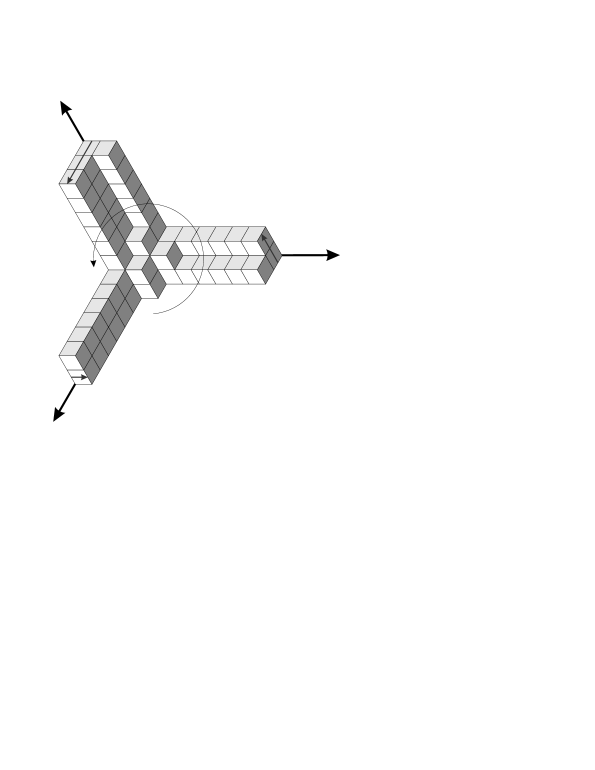
Figure 13: A one-dimensional ideal $I_{\pi}\in\mathbb{C}[x_{1},x_{2},x_{3}]$ corresponds to a 3-dimensional partitions that can have infinite legs in 3-coordinate directions. Just to label their asymptotic $2d$ partitions $\lambda_{\mathbf{e}}$, it is convenient to use the orientation of the figure that comes from the orientation of the $\Delta(X)$. In this example, $\lambda_{\mathbf{e}}\in\{(2,1),(3,1),(1,1)\}$.

Globally these partitions glue like in Figure 14, where the length of the edge should be considered as something much, much larger than the size of a box. For the 3-dimensional partitions to glue, their asymptotic partitions $\lambda_{\mathbf{e}}$ along the given edge have to match like

$$\lambda_{\overrightarrow{\mathbf{e}}}=\left(\lambda_{\overleftarrow{\mathbf{e}}}\right)^{\prime}$$

if one follows the conventions of Figure 13 and where prime denotes the transposed partition.

Figure 14: Two one-dimensional ideals glue on the overlap of two toric charts. The edge scheme $C_{\mathbf{e}}$ here is the line $\mathsf{L}_{\mathbf{e}}$ doubled in one of the coordinate directions.

6.2.3

If we take just this partition $\lambda_{\mathbf{e}}$ running along $\mathsf{L}_{\mathbf{e}}$, we get a canonically defined subscheme

$$C\supset C_{\mathbf{e}}=\overline{C\cap\mathbb{A}^{3}_{\mathsf{v}}\cap\mathbb{A}^{3}_{\mathsf{v}^{\prime}}}$$

where $\mathsf{v},\mathsf{v}^{\prime}$ are the two vertices joined by the edge $\mathbf{e}$. We have

$$\deg C_{\mathbf{e}}=|\lambda_{\mathbf{e}}|\deg\mathsf{L}_{e}$$

and

$$Q^{\deg C}=\prod_{\mathbf{e}\in\Delta(X)}(Q^{\deg\mathsf{L}_{\mathbf{e}}})^{|\lambda_{\mathbf{e}}|}$$

is the $Q^{d}$ weight of $C$ in partition functions (11) and (12).

6.3 Localization of DT counts

6.3.1

With the kinematics of $\mathsf{T}$-fixed subschemes sorted out, we now discuss the dynamics, that is, their weights in localization formulas. Just like in (97) we have

$$T^{\textup{vir}}_{C}=\mathscr{T}_{X}(\mathscr{I}_{C})$$

where $\mathscr{I}_{C}$ is the ideal sheaf of $C$ and where we denote

$$\mathscr{T}_{U}(\mathscr{F})=\chi(\mathscr{O}_{U})-\chi(\mathscr{F},\mathscr{F})\,,$$

for a coherent sheaf $\mathscr{F}$ on an open set $U\subset X$. It is convenient to have $\mathscr{T}_{U}(\mathscr{F})$ defined on opens because e.g. localization gives

$$T^{\textup{vir}}_{C}=\sum_{\mathsf{v}\in\Delta(X)}\mathscr{T}_{\mathbb{A}^{3}_{\mathsf{v}}}(I_{\pi_{\mathsf{v}}})\,.$$ (100)

Each term in (100) may be computed by the formula (99), where $\mathsf{G}_{\pi_{\mathsf{v}}}$ is now a rational function of $(t_{1},t_{2},t_{3})$. Similarly, $\mathscr{T}_{\mathbb{A}^{3}_{\mathsf{v}}}(I_{\pi_{\mathsf{v}}})$ is a rational function, and so the computation (100) is really taking place in the localized $\mathsf{T}$-equivariant K-theory. The torus $\mathsf{T}$ has no fixed points on double intersections of the charts $\mathbb{A}^{3}_{\mathsf{v}}$, which is why the corresponding terms are absent in the sum(100). Their $\mathsf{T}$-characters are torsion and vanish in the localization.

On the other hand, being a rational function makes $\mathscr{T}_{\mathbb{A}^{3}_{\mathsf{v}}}(I_{\pi_{\mathsf{v}}})$ unsuitable as an argument for $\widehat{\mathsf{a}}(\,\cdot\,)$. To remedy this, we literally subtract the contributions of the infinite legs as follows

$$\mathscr{T}^{\textup{vtx}}_{\pi_{\mathsf{v}}}=\mathscr{T}_{\mathbb{A}^{3}_{\mathsf{v}}}(I_{\pi_{\mathsf{v}}})-\sum_{\mathbf{e}}\mathscr{T}_{\mathbb{A}^{3}_{\mathsf{v}}}(I_{\mathbf{e}})$$ (101)

where the sum is over the edges $\mathbf{e}$ incident to $\mathsf{v}$ and $I_{\mathbf{e}}=\mathscr{I}_{C_{\mathbf{e}}}\big{|}_{\mathbb{A}^{3}_{\mathsf{v}}}$. It is easy to see this (101) is a polynomial in $t$.

By construction, this splits the virtual tangent space

$$T^{\textup{vir}}_{C}=\sum_{\mathbf{e}\in\Delta(X)}T^{\textup{vir}}_{C_{\mathbf{e}}}+\sum_{\mathsf{v}\in\Delta(X)}\mathscr{T}^{\textup{vtx}}_{\pi_{\mathsf{v}}}\,.$$ (102)

into the contributions of the edges curves $C_{\mathbf{e}}$ and their interaction at the vertices $\mathsf{v}$. This can be used to organize the localization formula as follows.

6.3.2

If $\lambda$ is a partition running along an edge $\mathbf{e}$, we define the corresponding edge weight by

$$\mathsf{E}_{\mathbf{e}}(\lambda)=(-z)^{\chi(\mathscr{O}_{C_{\mathbf{e}}})}\,Q^{|\lambda|\deg L_{\mathbf{e}}}\,\,\widehat{\mathsf{a}}\left(-T^{\textup{vir}}_{C_{\mathbf{e}}}\right)\,.$$

There is an elementary arm-and-leg expression for $T^{\textup{vir}}_{C_{\mathbf{e}}}$ that depends on the normal bundle $N_{X/\mathsf{L}_{e}}$. In particular, $\mathsf{E}_{\mathbf{e}}(\lambda)$ becomes the function $\mathbb{E}(\lambda,\lambda)$ from Section 3.3 when the normal bundle is trivial.

If $\lambda$, $\mu$, and $\nu$ are the partitions running along the three edges incident to a vertex $\mathsf{v}$ we define

$$\mathsf{V}_{\mathsf{v}}(\lambda,\mu,\nu)=\sum_{\textup{$\pi$ ending on $(\lambda,\mu,\nu)$}}(-z)^{|\pi|}\,\,\,\widehat{\mathsf{a}}\left(-\mathscr{T}^{\textup{vtx}}_{\pi}\right)$$ (103)

where $|\pi|$ is the regularized size of $\pi$, namely

$$|\pi|=\chi(C_{\pi})-\sum_{\mathbf{e}}\chi(C_{\mathbf{e}})\,,$$

which may be negative.

Note that (103) depends on the vertex $\mathsf{v}$ only through the assignment of equivariant variables. In other words, this is one universal function of 3 partition, 3 equivariant variables, and the box-counting variable $z$. It has an $S(3)$-symmetry that permutes/transposes partitions while permuting the equivariant variables.

6.3.3

With this notation, we can write the localization formula for curve counts in $X$ as a partition function of a vertex model, in which the degrees of freedom are partitions living on the edges of $\Delta(X)$ and their interaction happens at vertices. Concretely,

$$Z(X)=\sum_{\textup{all maps $\mathbf{e}\to\lambda_{e}$}}\prod_{\mathbf{e}}\mathsf{E}_{\mathbf{e}}(\lambda_{\mathbf{e}})\prod_{\mathsf{v}}\mathsf{V}_{\mathsf{v}}(\lambda_{\mathbf{e}_{1}},\lambda_{\mathbf{e}_{2}},\lambda_{\mathbf{e}_{3}})$$ (104)

where $\mathbf{e}_{i}$ are the three edges incident to $\mathsf{v}$.

6.3.4

Formulas of the form (104) have a long history in the subject, starting from the topological vertex conjecture of [AKMV]. In there, Aganagic, Klemm, Mariño, and Vafa proposed a formula, with the same structure, for GW counts in toric CY threefolds. The topological vertex of [AKMV] is an explicit expression with Schur functions inspired by a connection to knot invariants from Section 3.2.3.

Note that in the Calabi-Yau case, we have

$$T^{\textup{vir}}=-\left(T^{\textup{vir}}\right)^{\vee}$$

equivariantly. Hence $\widehat{\mathsf{a}}(T^{\textup{vir}})=\pm 1$ and the summation in (104) becomes pure combinatorics of boxcounting. From a modern point of view, this combinatorics had just been sorted out at the time in [OR], and so once one knew there is a connection it was easy to see that

$$\textup{topological vertex}=\sum_{\textup{$\pi$ ending on $(\lambda,\mu,\nu)$}}z^{|\pi|}\,,\quad z=e^{iu}\,.$$

This is the main point of [ORV] and it was also explained there that boxcounting is related to the Hilbert scheme of curves in 3-dimensions. An early discussion of a 3-dimensional analog of Nekrasov theory may be found in a related paper [Iqbal].

All of this was a very important inspiration for [MNOP1, MNOP2], where the general GW/DT correspondence was proposed and where it was explained how it specializes to the topological vertex formula for toric CY threefolds.

6.3.5

Formulas like (104) have an obvious gauge symmetry. They can be seen as a contraction of certain tensors in

$$\mathsf{Fock}^{\otimes\textup{edges of $\Delta(X)$}}(t_{1},t_{2},t_{3})(\!(z)\!)$$

where $\mathsf{Fock}$ is a vector space with a basis given by partitions. Clearly, we are free to change the basis in any tensor factor without affecting the result.

In (104), the edge terms are explicit products and the whole complexity sits at vertices. The capped localization of [57], is a gauge transformation that spreads the complexity more evenly. In capped localization, edge terms corresponds to deformations of $C_{\mathbf{e}}$ considered relative to the two toric divisors at the endpoints of $\mathsf{L}_{\mathbf{e}}$, and similarly, the vertex terms are considered relative infinity which may be modeled by the infinity of

$$\mathbb{A}^{3}\subset(\mathbb{P}^{1})^{3}\,.$$

The equivalence with (104) follows from the degeneration formula of Section 2.3.

6.3.6

In capped localization, the edge terms are well-controlled rational functions of $z$ that absorb some of the complexity from

$$\frac{\mathsf{V}(\lambda,\mu,\nu)_{\textup{capped}}}{\mathsf{V}(\varnothing,\varnothing,\varnothing)} =\textup{a rational function of $z$, in fact}$$ (105)

$$\overset{?}{=}\textup{a Laurent polynomial in $z$}\,.$$ (106)

The rationality (105), which is the analog of the Conjecture (1), is proven in [57] along the lines that will be explained shortly. In fact, one of our main goal in the rest of these notes is to explain how one computes this function.

The polynomiality in (105) remains a conjecture.

6.3.7

Localization in PT theory takes a very similar shape, see [PT2]. The fixed loci now have much fewer components, but may be not isolated if $\lambda,\mu,\nu$ are all nonempty.

6.3.8

The shape of localization formulas in GW theory is structurally very similar. Let

$$f:C=\bigcup C_{i}\to X$$

be a $\mathsf{T}$-fixed stable map, where $\{C_{i}\}$ are irreducible components of the source curve $C$. For each $C_{i}$, there are two possibilities:

• if $C_{i}$ is not contracted by $f$, then $f|_{C_{i}}$ has the form

  $$C_{i}\cong\mathbb{P}^{1}\owns y\xrightarrow{\,\,f\,\,}y^{\mu_{i}}\in\mathbb{P}^{1}\cong\mathsf{L}_{\mathbf{e}}$$

  for some edge $\mathbf{e}$ and some degree $\mu_{i}=1,2,\dots$. For every edge, these degrees form a partition $\mu_{\mathbf{e}}$. The contribution of such $C_{i}$ to the virtual tangent space is simple and explicit.

• otherwise, $C_{i}$ is contracted by $f$ to a vertex $\mathsf{v}$. These components contribute an analog of (70), but now with 3 Chern classes of the Hodge bundle.

There is, similarly, a capped version of the localization available. The proof of the GW/DT correspondence for toric varieties [57] really matches the capped GW vertices and edges to their cohomological counterparts in DT theory.

Figure 15: The shape of torus fixed stable maps to $X$, compare with Figures 10 and 13.

6.4 $A_{n}$-geometries capture vertices

6.4.1

The vertex (103) is a basic building block of the theory and a very important special function. One can view it as a tensor

$$\mathsf{V}\in(\mathsf{Fock})^{\otimes 3}\otimes\mathbb{Q}(t)(\!(z)\!)$$ (107)

and contemplate determining it by the representation theory of a suitable algebra acting in this linear space, like it was done in [ADKMV, AFS] for the topological vertex, and the so called refined topological vertex, which is also a (very) special case of (103).

While this is a very important direction of current research, it turns out to be easier to repackage this tensor differently, as a certain different 3-valent tensor that can be determined by representation theory of a certain quantum group. This group is $\mathscr{U}_{\hbar}(\widehat{\widehat{\mathfrak{gl}}}_{3})$, which is a quantum loop group associated to the loop algebra $\widehat{\mathfrak{gl}}_{3}$, see [84] for an introduction. There is, in fact, a sequence of $n$-valent tensors that similarly correspond to $\widehat{\mathfrak{gl}}_{n}$ for all $n$. They correspond to

$$X_{n}=A_{n-1}\times\mathbb{A}^{1}\,,\quad n=1,2,\dots\,,$$ (108)

where $A_{n-1}$ is the toric symplectic surface we met previously in Section 5.5.6.

The vertex (107) has a nice $S(3)$-covariance, but the fact that its three legs point in three different coordinate directions makes it more difficult for the three tensor factors in (107) to interact.

6.4.2

We have

$$A_{1}=T^{*}\mathbb{P}^{1}$$

and the toric polyhedron $\Delta(X_{2})$ is drawn in Figure 16.

Figure 16: The $1$-skeleton of $\Delta(X_{2})$ has a unique bounded edge and the corresponding partition function (109) is a sum over the unique intermediate partition $\eta$.

We assign the partitions $\varnothing$, $\lambda$, $\mu$, and $\varnothing$ to the unbounded edges and consider

$$\mathsf{Z}(X_{2},\lambda,\mu\,|\,z,Q)=\sum_{\eta}\mathsf{E}(\eta)\,\mathsf{V}(\varnothing,\mu,\eta^{\prime})\,\mathsf{V}(\eta,\lambda,\varnothing)\,.$$ (109)

where the new variable $Q$ enters through the $Q^{|\eta|}$ part of the edge weight $\mathsf{E}(\eta)$ in (109). The coefficient $Q^{k}$ thus restricts the summation to $|\eta|=k$.

The sum (109) may be seen as the partition function for $A_{1}\times\mathbb{P}^{1}$ with nonsingular boundary conditions imposed at the divisor $A_{1}\times\{\infty\}$.

Lemma 6.2 ([57]).

The function (109) uniquely determines the vertices with one of the 3 partitions empty.

Proof.

Suppose we want to compute $\mathsf{V}(\eta,\lambda,\varnothing)$. By symmetry and induction, we can assume $|\eta|\leq|\lambda|$. Viewing (109) as linear equations on the unknowns $\{\mathsf{V}(\eta,\lambda,\varnothing)\}$, it suffices to check that the matrix

$$\left(\mathsf{V}(\varnothing,\mu,\eta^{\prime})\right)_{|\mu|<k\,,|\eta|=k}$$

has maximal rank for $k=1,2,\dots$. It is enough to check this for the topological vertex specialization, and this was done in [57]. ∎

6.4.3

It is now clear that the same argument applied to

$$X_{3}=A_{2}\times\mathbb{A}^{1}$$

will capture the full 3-valent vertex with one of the outgoing edges equal to $\mu$.

Figure 17: The topic polytope for $X_{3}$.

As a result, the function $\mathsf{Z}(X_{3},\lambda,\mu,\nu)$ contains $\mathsf{V}$ in an effective way, from which properties like rationality in $z$ may be concluded.

Clearly, $\mathsf{Z}(X_{3},\lambda,\mu,\nu)$ a richer function since it depends on $Q_{1}$ and $Q_{2}$ for the two curve classes in $A_{2}$. It is therefore remarkable that this function, and its $n$-valent generalization for $X_{n}$ may be described explicitly in the language of geometric representation theory.

7 DT counts in ADE fibrations

7.1 Quasimaps again

7.1.1

The ADE surfaces $S$, minimal resolutions of

$$\textup{ADE singularities}=\mathbb{A}^{2}/\Gamma\,,$$

where $\Gamma\subset SL_{2}(\mathbb{C})$ is a finite subgroup, are some of the nicest objects in the theory of surfaces and very often make an appearance in other parts of mathematics.

What unites them from our point of view is that their Hilbert schemes are Nakajima varieties [Nakq1]. Therefore if $X$ is an ADE fibration

$$\lx@xy@svg{\hbox{\raise 0.0pt\hbox{\kern 6.35416pt\hbox{\ignorespaces\ignorespaces\ignorespaces\hbox{\vtop{\kern 0.0pt\offinterlineskip\halign{\entry@#!@&&\entry@@#!@\cr&\\&\crcr}}}\ignorespaces{\hbox{\kern-6.35416pt\raise 0.0pt\hbox{\hbox{\kern 0.0pt\raise 0.0pt\hbox{\hbox{\kern 3.0pt\raise 0.0pt\hbox{$\textstyle{S\ignorespaces\ignorespaces\ignorespaces\ignorespaces}$}}}}}}}\ignorespaces\ignorespaces\ignorespaces\ignorespaces{\hbox{\kern 6.35416pt\raise 0.0pt\hbox{\hbox{\kern 0.0pt\raise 0.0pt\hbox{\lx@xy@hook{1}}}}}}{\hbox{\lx@xy@droprule}}\ignorespaces{\hbox{\kern 30.35416pt\raise 0.0pt\hbox{\hbox{\kern 0.0pt\raise 0.0pt\hbox{\lx@xy@tip{1}\lx@xy@tip{-1}}}}}}{\hbox{\lx@xy@droprule}}{\hbox{\lx@xy@droprule}}{\hbox{\kern 30.35416pt\raise 0.0pt\hbox{\hbox{\kern 0.0pt\raise 0.0pt\hbox{\hbox{\kern 3.0pt\raise 0.0pt\hbox{$\textstyle{X\ignorespaces\ignorespaces\ignorespaces\ignorespaces}$}}}}}}}\ignorespaces\ignorespaces\ignorespaces\ignorespaces{}{\hbox{\lx@xy@droprule}}\ignorespaces\ignorespaces\ignorespaces{\hbox{\kern 37.88887pt\raise-18.41666pt\hbox{{}\hbox{\kern 0.0pt\raise 0.0pt\hbox{\hbox{\kern 3.0pt\hbox{\hbox{\kern 0.0pt\raise-1.50694pt\hbox{$\scriptstyle{\pi}$}}}\kern 3.0pt}}}}}}\ignorespaces{\hbox{\kern 37.88887pt\raise-27.0pt\hbox{\hbox{\kern 0.0pt\raise 0.0pt\hbox{\lx@xy@tip{1}\lx@xy@tip{-1}}}}}}{\hbox{\lx@xy@droprule}}{\hbox{\lx@xy@droprule}}{\hbox{\kern-3.0pt\raise-36.83331pt\hbox{\hbox{\kern 0.0pt\raise 0.0pt\hbox{\hbox{\kern 3.0pt\raise 0.0pt\hbox{$\textstyle{}$}}}}}}}{\hbox{\kern 30.84547pt\raise-36.83331pt\hbox{\hbox{\kern 0.0pt\raise 0.0pt\hbox{\hbox{\kern 3.0pt\raise 0.0pt\hbox{$\textstyle{B}$}}}}}}}\ignorespaces}}}}\ignorespaces\,, \textstyle{S\ignorespaces\ignorespaces\ignorespaces\ignorespaces} \textstyle{X\ignorespaces\ignorespaces\ignorespaces\ignorespaces} \scriptstyle{\pi} \textstyle{B} \textstyle{S\ignorespaces\ignorespaces\ignorespaces\ignorespaces} \textstyle{X\ignorespaces\ignorespaces\ignorespaces\ignorespaces} \scriptstyle{\pi} \textstyle{B}$$ (110)

like what we have already seen in Section 5.5.6, then one can study quasimap sections of the corresponding fibration of the Hilbert schemes

$$\lx@xy@svg{\hbox{\raise 0.0pt\hbox{\kern 19.54863pt\hbox{\ignorespaces\ignorespaces\ignorespaces\hbox{\vtop{\kern 0.0pt\offinterlineskip\halign{\entry@#!@&&\entry@@#!@\cr&\\&\crcr}}}\ignorespaces{\hbox{\kern-19.54863pt\raise 0.0pt\hbox{\hbox{\kern 0.0pt\raise 0.0pt\hbox{\hbox{\kern 3.0pt\raise 0.0pt\hbox{$\textstyle{\operatorname{Hilb}(S)\ignorespaces\ignorespaces\ignorespaces\ignorespaces}$}}}}}}}\ignorespaces\ignorespaces\ignorespaces\ignorespaces{\hbox{\kern 19.54865pt\raise 0.0pt\hbox{\hbox{\kern 0.0pt\raise 0.0pt\hbox{\lx@xy@hook{1}}}}}}{\hbox{\lx@xy@droprule}}\ignorespaces{\hbox{\kern 43.54863pt\raise 0.0pt\hbox{\hbox{\kern 0.0pt\raise 0.0pt\hbox{\lx@xy@tip{1}\lx@xy@tip{-1}}}}}}{\hbox{\lx@xy@droprule}}{\hbox{\lx@xy@droprule}}{\hbox{\kern 43.54863pt\raise 0.0pt\hbox{\hbox{\kern 0.0pt\raise 0.0pt\hbox{\hbox{\kern 3.0pt\raise 0.0pt\hbox{$\textstyle{\operatorname{Hilb}(\pi)\ignorespaces\ignorespaces\ignorespaces\ignorespaces}$}}}}}}}\ignorespaces\ignorespaces\ignorespaces\ignorespaces{}{\hbox{\lx@xy@droprule}}\ignorespaces{\hbox{\kern 62.59325pt\raise-28.58334pt\hbox{\hbox{\kern 0.0pt\raise 0.0pt\hbox{\lx@xy@tip{1}\lx@xy@tip{-1}}}}}}{\hbox{\lx@xy@droprule}}{\hbox{\lx@xy@droprule}}{\hbox{\kern-3.0pt\raise-38.41666pt\hbox{\hbox{\kern 0.0pt\raise 0.0pt\hbox{\hbox{\kern 3.0pt\raise 0.0pt\hbox{$\textstyle{}$}}}}}}}{\hbox{\kern 55.54985pt\raise-38.41666pt\hbox{\hbox{\kern 0.0pt\raise 0.0pt\hbox{\hbox{\kern 3.0pt\raise 0.0pt\hbox{$\textstyle{B\ignorespaces\ignorespaces\ignorespaces\ignorespaces\ignorespaces}$}}}}}}}\ignorespaces\ignorespaces\ignorespaces\ignorespaces\ignorespaces{}{}{}{{}{}{}{}{}{}{}{}{}{}{}{}{}{}{}{}{}}{}\ignorespaces\hbox{\hbox{\kern 0.0pt\raise 0.0pt\hbox{{}{}{{}}{{}{}{}}{}}}}\ignorespaces{}\ignorespaces{}{}{}{{}{}}\ignorespaces\ignorespaces{\hbox{\kern 86.59325pt\raise-19.20834pt\hbox{{}\hbox{\kern 0.0pt\raise 0.0pt\hbox{\hbox{\kern 3.0pt\hbox{\hbox{\kern 0.0pt\raise-1.75pt\hbox{$\scriptstyle{f}$}}}\kern 3.0pt}}}}}}\ignorespaces{}{}{}{{}{}{}{}{}{}{}{}{}{}{}{}{}{}{}{}{}{}{}}{\hbox{\kern 74.3627pt\raise-5.49619pt\hbox{\hbox{\kern 0.0pt\raise 0.0pt\hbox{\lx@xy@tip{1}\lx@xy@tip{-1}}}}}}\ignorespaces\hbox{\hbox{\kern 0.0pt\raise 0.0pt\hbox{{}{}{}{{}}{{}{}{}\lx@xy@spline@}{}}}}\ignorespaces{}\ignorespaces\hbox{\hbox{\kern 0.0pt\raise 0.0pt\hbox{{}{}{{}}{{}{}{}}{}}}}\ignorespaces{}\ignorespaces}}}}\ignorespaces\,, \textstyle{\operatorname{Hilb}(S)\ignorespaces\ignorespaces\ignorespaces\ignorespaces} \textstyle{\operatorname{Hilb}(\pi)\ignorespaces\ignorespaces\ignorespaces\ignorespaces} \textstyle{B\ignorespaces\ignorespaces\ignorespaces\ignorespaces\ignorespaces} \scriptstyle{f} \textstyle{\operatorname{Hilb}(S)\ignorespaces\ignorespaces\ignorespaces\ignorespaces} \textstyle{\operatorname{Hilb}(\pi)\ignorespaces\ignorespaces\ignorespaces\ignorespaces} \textstyle{B\ignorespaces\ignorespaces\ignorespaces\ignorespaces\ignorespaces} \scriptstyle{f}$$ (111)

like we did in Section 5.5.3.

7.1.2

If $S=\mathbb{A}^{2}$ then these quasimap moduli spaces are the PT moduli spaces. In general, they are even more economical than the PT moduli spaces and, by transitivity, much more economical than the Hilbert schemes of curves in $X$.

Quasimap counting also has a noticeable technical advantage in how it can handle sheaves of higher rank on $X$. Recall from Section 5.5.6 that the moduli of rank $r$ torsion free sheaves on $S$ are also Nakajima varieties, and so one can just count quasimaps to those.

Counting quasimaps in (111) is just another flavor of DT theory of X and is expected to be related to other counts by a simple wall-crossing like (15). In cohomology, this comes out for free from the results of [57, MObl], and situation in equivariant K-theory should be similar.

7.1.3

Since it is easier to work with quasimaps, and K-theoretic counts are complicated enough, so far people focused on doing them for quasimaps. There is now a satisfactory general enumerative theory of quasimaps to general Nakajima varieties, see [84, 85] for an introduction and overview.

7.1.4

The base $B$ in (110) is a fixed nonsingular curve. By deformation invariance and gluing, the DT counts relative the fibers of (110), that is, the assignment

$$(B,\{b_{i}\})\mapsto\mathsf{Z}(X/D)\,,\quad D=\pi^{-1}(\{b_{i}\})$$ (112)

defines a 2-dimensional TQFT and, more generally, a K-theoretic analog of a cohomological field theory if the curve $B$ is allowed to move in families.

The space of boundary conditions in this TQFT is (20) in cohomology and

$$K_{\operatorname{Aut}(S)}(\operatorname{Hilb}(S))=\bigoplus_{k}K_{\operatorname{Aut}(S)}(\operatorname{Hilb}(S),k)$$ (113)

in equivariant $K$-theory.

7.1.5

More precisely, this is a TQFT that is further enriched to keep track of the topology of the bundle in (110) which is labelled by a cocharacter

$$\sigma:\mathbb{C}^{\times}\to\operatorname{Aut}(S)\,.$$ (114)

In degeneration, the bundle degree may be split arbitrarily between the components.

It is convenient to treat bundle topology as the action of commuting shift operators indexed by $\sigma$. In higher rank, there are similar shift operators related to the framing automorphisms of Nakajima varieties.

7.1.6

There is a simple Lie algebra $\mathfrak{g}_{\textup{\tiny{ADE}}}$ associated to $S$ and the corresponding affine Lie algebra

$$\mathfrak{g}_{\textup{\tiny{KM}}}=\textup{central extension of }\mathfrak{g}_{\textup{\tiny{ADE}}}[x^{\pm 1}]$$ (115)

is an example of a Kac-Moody Lie algebra. By the work of Nakajima [Nak3], (113) is a module for $\mathscr{U}_{\hbar}(\widehat{\mathfrak{g}}_{\textup{\tiny{KM}}})$, which is a quantum loop group algebra associated to the Kac-Moody Lie algebra (115).

Note that we are dealing here with quantum double loop symmetries, something that has many more layers of representation-theoretic complexity than the affine Lie algebra or the ordinary (non-loop) quantum groups of the CS theory.

7.1.7

From a geometric R-matrix perspective, an abstract Lie algebra $\mathfrak{g}_{\textup{\tiny{MO}}}$ was associated in [58] to any quiver so that $\mathscr{U}_{\hbar}(\widehat{\mathfrak{g}}_{\textup{\tiny{MO}}})$ acts on equivariant K-theories of Nakajima quiver varieties, see [93, 84]. This extends the action of $\mathscr{U}_{\hbar}(\widehat{\mathfrak{g}}_{\textup{\tiny{KM}}})$ constructed by Nakajima in [Nak3].

For quivers of affine ADE type, the difference between the two Lie algebras is a single Heisenberg algebra $\widehat{\mathfrak{gl}}_{1}$. For example

$$\mathfrak{g}_{\textup{\tiny{KM}}}=\widehat{\mathfrak{sl}}_{n+1}\subset\widehat{\mathfrak{gl}}_{n+1}=\mathfrak{g}_{\textup{\tiny{MO}}}$$

for quivers of affine $A_{n}$-type that correspond to Hilbert schemes of $A_{n}$-surfaces. It is the action of $\mathscr{U}_{\hbar}(\widehat{\mathfrak{g}}_{\textup{\tiny{MO}}})$ that will be required to do the quasimap counts and the main motivation for [58] were precisely enumerative applications.

7.2 Representation theory answers

7.2.1

From the TQFT principles, it suffices to do the counts (112) for $B=\mathbb{P}^{1}$ with at most 3 marked points $\{b_{1},\dots,b_{n}\}$. The counts with $n\leq 2$ marked points can be done equivariantly with respect to $\operatorname{Aut}(B,\{b_{i}\})$. In fact, this makes $\leq 2$-point counts so rich that they determine all other ones by elementary operations.

Recall from Section 2 that we have several options for the boundary conditions to impose at $\pi^{-1}(\{b_{i}\})$. Namely, we can impose the nonsingular, relative, and descendent boundary conditions, see Section 2.2. Counts with 2-marked points and different flavors of boundary conditions provide the dictionary between the insertions as in Section 2.4.

Different flavors of insertions results in objects of different geometric, analytic (as functions of parameters), and representation-theoretic flavors. We now list various possibilities, first taking the $S$-bundle in (110) to be trivial.

7.2.2 One nonsingular point

This is the count of Section 6.4, le raison d’etre of this section. By change of the boundary condition, it corresponds to:

7.2.3 One relative point

This count is trivial, in the sense that this is identity element (structure sheaf $\mathscr{O}_{\operatorname{Hilb}}$) in (113), up to normalizations.

While the count is trivial, this triviality is in itself highly nontrivial as it involves the vanishing of many quantum corrections that are not constrained to vanish for simple reasons like dimension. Here, we have an instance of what was called large rank vanishing in [84], something which also holds for counts of Section 7.2.5 once the rank becomes large compared to the size of the descendent insertion.

What relates this simple answer to Section 7.2.2 is the following change of basis matrix:

7.2.4 Two points: one relative, one nonsingular

This is a fundamental solutions of a certain system of $q$-difference equations in all other variables. Here

$$q\in\mathbb{C}^{\times}=\operatorname{Aut}(B,\{b_{1},b_{2}\})$$

and the equations are written using the operators of

$$\mathscr{U}_{\hbar}=\mathscr{U}_{\hbar}(\widehat{\mathfrak{g}}_{\textup{\tiny{MO}}})\,,$$

see [93, 84, 85].

The equations in the variables $z$ and $Q$ found in [93] may be described as a certain deformation of the action of what may be called the affine Weyl group of $\mathscr{U}_{\hbar}$. Beware, however, that in the non-Kac-Moody situation we are really talking not about a group but about the fundamental groupoid of a certain hyperplane arrangement, namely the arrangement associated to the roots of $\widehat{\mathfrak{g}}_{\textup{\tiny{MO}}}$. This arrangement is very far from being the arrangement of reflection hyperplanes for a discrete reflection group. In particular, its symmetries, which apriori include only a lattice of translations and the reflection about the origin, do not act transitively on the set of alcoves.

For instance, for $\operatorname{Hilb}(\mathbb{A}^{2},k)$, this is a $1$-dimensional arrangement with hyperplanes $mx\in\mathbb{Z}$ for $m=1,\dots,k$, where $x$ is the coordinate. This kind of combinatorics replaces Weyl group symmetries in the subject, see [85] for a discussion.

A fundamental solution to a $q$-difference equations may be interpreted as a (regularized) infinite product of certain wall-crossing operators that cross all walls between a certain alcove and a point at infinity.

7.2.5 Two points: one relative, one descendent

There are explicit answers for these counts, too, see [3, 103]. By general principles, they give a dictionary between relative and descendent insertions, something which is very useful for accessing DT counts in general threefolds.

They also related the subject of Bethe Ansatz for $\mathscr{U}_{\hbar}$, because they relate the counts of Section 7.2.4 to the following:

7.2.6 Two points: one descendent, one nonsingular

These counts may be given by an explicit Mellin-Barnes-type intergral because the $q$-fixed quasimaps are GIT quotients, see [1]. Integral solutions for $q$-difference equations turn into formulas for eigenfunctions in the $q\to 1$ limit and this is the subject of Bethe Ansatz for $\mathscr{U}_{\hbar}$. Geometric considerations solve the problem completely, giving, in particular, a concise explicit formula for general off-shell Bethe eigenfunction, see [3].

Of course, the corresponding eigenvalues were understood long time ago by Nekrasov and Shatashvili in [NS1, NS2]. That very influential work was what stimulated the interest in quasimap counts in the first place, see e.g. [58] for a longer discussion.

7.2.7 Two point, both relative, nontrivial bundle

This is the shift operator corresponding to the degree $\sigma$ of the bundle in (114). They give the $q$-difference equations from Section 7.2.4 in the corresponding equivariant variables.

These operators, as well as the difference equations in $z$ and $Q$, are all found from the their consistency with $q$-difference equations in variables $a_{i}$ that appear in higher rank counts exactly as they appeared in (44). The difference equations in $a_{i}$ are identified as the quantum Knizhnik-Zamolodchikov equations [FrenResh] for $\mathscr{U}_{\hbar}$ in [84], and this is really the point through which the powerful machinery of geometric representations theory enters the world of counting.

References

- [1] M. Aganagic, E. Frenkel, and A. Okounkov, Quantum -Langlands Correspondence, arXiv:1701.03146.
- [2] M. Aganagic and A. Okounkov, Elliptic stable envelopes, arXiv:1604.00423.
- [3] \bysame, Quasimap counts and Bethe eigenfunctions, arXiv:1704.08746.
- [4] \bysame, in preparation. AganagicM.KlemmA.MariñoM.VafaC.The topological vertexComm. Math. Phys.25420052425–478ISSN 0010-3616@article{AKMV, author = {Aganagic, M.}, author = {Klemm, A.}, author = {Mari\~no, M.}, author = {Vafa, C.}, title = {The topological vertex}, journal = {Comm. Math. Phys.}, volume = {254}, date = {2005}, number = {2}, pages = {425–478}, issn = {0010-3616}} AganagicMinaDijkgraafRobbertKlemmAlbrechtMariñoMarcosVafaCumrunTopological strings and integrable hierarchiesComm. Math. Phys.26120062451–516@article{ADKMV, author = {Aganagic, Mina}, author = {Dijkgraaf, Robbert}, author = {Klemm, Albrecht}, author = {Mari\~no, Marcos}, author = {Vafa, Cumrun}, title = {Topological strings and integrable hierarchies}, journal = {Comm. Math. Phys.}, volume = {261}, date = {2006}, number = {2}, pages = {451–516}} AtiyahM.Topological quantum field theoriesInst. Hautes Études Sci. Publ. Math.681988175–186 (1989)ISSN 0073-8301@article{AtTQFT, author = {Atiyah, M.}, title = {Topological quantum field theories}, journal = {Inst. Hautes \'Etudes Sci. Publ. Math.}, number = {68}, date = {1988}, pages = {175–186 (1989)}, issn = {0073-8301}} AwataH.FeiginB.ShiraishiJ.Quantum algebraic approach to refined topological vertexJ. High Energy Phys.20123041, front matter+34@article{AFS, author = {Awata, H.}, author = {Feigin, B.}, author = {Shiraishi, J.}, title = {Quantum algebraic approach to refined topological vertex}, journal = {J. High Energy Phys.}, date = {2012}, number = {3}, pages = {041, front matter+34}} BaggerJ.LambertN.MukhiS.PapageorgakisC.Multiple membranes in m-theoryPhys. Rep.527201311–100ISSN 0370-1573@article{MMM, author = {Bagger, J.}, author = {Lambert, N.}, author = {Mukhi, S.}, author = {Papageorgakis, C.}, title = {Multiple membranes in M-theory}, journal = {Phys. Rep.}, volume = {527}, date = {2013}, number = {1}, pages = {1–100}, issn = {0370-1573}} BakalovB.Kirillov Jr.A.Lectures on tensor categories and modular functorsUniversity Lecture Series21American Mathematical Society, Providence, RI2001x+221@book{BakKir, author = {Bakalov, B.}, author = {Kirillov Jr., A.}, title = {Lectures on tensor categories and modular functors}, series = {University Lecture Series}, volume = {21}, publisher = {American Mathematical Society, Providence, RI}, date = {2001}, pages = {x+221}} BakkerB.JorzaA.Higher rank stable pairs on k3 surfacesCommun. Number Theory Phys.620124805–847ISSN 1931-4523@article{Bakk, author = {Bakker, B.}, author = {Jorza, A.}, title = {Higher rank stable pairs on K3 surfaces}, journal = {Commun. Number Theory Phys.}, volume = {6}, date = {2012}, number = {4}, pages = {805–847}, issn = {1931-4523}}
- [12] K. Behrend and B. Fantechi, The intrinsic normal cone, Invent. Math. 128 (1997), no. 1, 45–88.
- [13] J. de Boer, K. Hori, H. Ooguri, Y. Oz, Mirror symmetry in three-dimensional gauge theories, quivers and D-branes, Nuclear Phys. B 493 (1997), no. 1-2, 101–147.
- [14] T. Braden, A. Licata, N. Proudfoot, B. Webster, Gale duality and Koszul duality, Adv. Math. 225 (2010), no. 4, 2002–2049.
- [15] T. Braden, A. Licata, N. Proudfoot, B. Webster, Quantizations of conical symplectic resolutions II: category and symplectic duality, arXiv:1407.0964.
- [16] A. Braverman, M. Finkelberg, H. Nakajima, Towards a mathematical definition of Coulomb branches of -dimensional gauge theories, II, arXiv:1601.03586.
- [17] A. Braverman, M. Finkelberg, H. Nakajima, Coulomb branches of quiver gauge theories and slices in the affine Grassmannian, arXiv:1604.03625. BridgelandT.Stability conditions on triangulated categoriesAnn. of Math. (2)16620072317–345ISSN 0003-486X@article{Br1, author = {Bridgeland, T.}, title = {Stability conditions on triangulated categories}, journal = {Ann. of Math. (2)}, volume = {166}, date = {2007}, number = {2}, pages = {317–345}, issn = {0003-486X}}
- [19] \bysame, Spaces of stability conditions, Algebraic geometry, Seattle 2005, Part 1, 1–21, AMS, 2009.
- [20] \bysame, Hall algebras and Donaldson-Thomas invariants, arXiv:1611.03696. BryanJ.PandharipandeR.The local gromov-witten theory of curvesWith an appendix by Bryan, C. Faber, A. Okounkov and PandharipandeJ. Amer. Math. Soc.2120081101–136ISSN 0894-0347@article{BrPand, author = {Bryan, J.}, author = {Pandharipande, R.}, title = {The local Gromov-Witten theory of curves}, note = {With an appendix by Bryan, C. Faber, A. Okounkov and Pandharipande}, journal = {J. Amer. Math. Soc.}, volume = {21}, date = {2008}, number = {1}, pages = {101–136}, issn = {0894-0347}}
- [22] M. Bullimore, T. Dimofte, and D. Gaiotto, The Coulomb Branch of 3d Theories, arXiv:1503.04817.
- [23] M. Bullimore, T. Dimofte, D. Gaiotto, and J. Hilburn, Boundaries, Mirror Symmetry, and Symplectic Duality in 3d Gauge Theory, arXiv:1603.08382.
- [24] N. Chriss and V. Ginzburg, Representation theory and complex geometry, Birkhäuser, Boston, 2010.
- [25] I. Ciocan-Fontanine, B. Kim, and D. Maulik, Stable quasimaps to GIT quotients, J. Geom. Phys. 75 (2014), 17–47. CarlsonF.Über potenzreihen mit ganzzahligen koeffizientenGermanMath. Z.919211-21–13ISSN 0025-5874@article{FritzC, author = {Carlson, F.}, title = {\"Uber Potenzreihen mit ganzzahligen Koeffizienten}, language = {German}, journal = {Math. Z.}, volume = {9}, date = {1921}, number = {1-2}, pages = {1–13}, issn = {0025-5874}} CarlssonE.OkounkovA.Exts and vertex operatorsDuke Math. J.161201291797–1815ISSN 0012-7094@article{CarOk, author = {Carlsson, E.}, author = {Okounkov, A.}, title = {Exts and vertex operators}, journal = {Duke Math. J.}, volume = {161}, date = {2012}, number = {9}, pages = {1797–1815}, issn = {0012-7094}} CerfR.KenyonR.The low-temperature expansion of the wulff crystal in the 3d ising modelComm. Math. Phys.22220011147–179ISSN 0010-3616@article{CerfK, author = {Cerf, R.}, author = {Kenyon, R.}, title = {The low-temperature expansion of the Wulff crystal in the 3D Ising model}, journal = {Comm. Math. Phys.}, volume = {222}, date = {2001}, number = {1}, pages = {147–179}, issn = {0010-3616}} DonaldsonS. K.Instantons and geometric invariant theoryComm. Math. Phys.9319844453–460ISSN 0010-3616@article{DonGIT, author = {Donaldson, S. K.}, title = {Instantons and geometric invariant theory}, journal = {Comm. Math. Phys.}, volume = {93}, date = {1984}, number = {4}, pages = {453–460}, issn = {0010-3616}} DonaldsonS. K.KronheimerP. B.The geometry of four-manifoldsOxford Mathematical MonographsOxford Science PublicationsThe Clarendon Press, Oxford University Press, New York1990x+440@book{DonKr, author = {Donaldson, S. K.}, author = {Kronheimer, P. B.}, title = {The geometry of four-manifolds}, series = {Oxford Mathematical Monographs}, note = {Oxford Science Publications}, publisher = {The Clarendon Press, Oxford University Press, New York}, date = {1990}, pages = {x+440}} DonaldsonS. K.ThomasR. P.Gauge theory in higher dimensionstitle={The geometric universe}, address={Oxford}, date={1996}, publisher={Oxford Univ. Press, Oxford}, 199831–47@article{DonTh, author = {Donaldson, S. K.}, author = {Thomas, R. P.}, title = {Gauge theory in higher dimensions}, conference = {title={The geometric universe}, address={Oxford}, date={1996}, }, book = {publisher={Oxford Univ. Press, Oxford}, }, date = {1998}, pages = {31–47}} FaberC.PandharipandeR.Hodge integrals and gromov-witten theoryInvent. Math.13920001173–199ISSN 0020-9910@article{FP, author = {Faber, C.}, author = {Pandharipande, R.}, title = {Hodge integrals and Gromov-Witten theory}, journal = {Invent. Math.}, volume = {139}, date = {2000}, number = {1}, pages = {173–199}, issn = {0020-9910}}
- [33] B. Fantechi and L. Göttsche, Riemann-Roch theorems and elliptic genus for virtually smooth schemes, Geom. Topol. 14 (2010), no. 1, 83–115. FantechiBarbaraGöttscheLotharIllusieLucKleimanSteven L.NitsureNitinVistoliAngeloFundamental algebraic geometryMathematical Surveys and Monographs123Grothendieck’s FGA explainedAmerican Mathematical Society, Providence, RI2005x+339@collection{FDA, author = {Fantechi, Barbara}, author = {G{\"o}ttsche, Lothar}, author = {Illusie, Luc}, author = {Kleiman, Steven L.}, author = {Nitsure, Nitin}, author = {Vistoli, Angelo}, title = {Fundamental algebraic geometry}, series = {Mathematical Surveys and Monographs}, volume = {123}, note = {Grothendieck's FGA explained}, publisher = {American Mathematical Society, Providence, RI}, date = {2005}, pages = {x+339}} FrenkelI.ReshetikhinN.Quantum affine algebras and holonomic difference equationsComm. Math. Phys.146199211–60@article{FrenResh, author = {Frenkel, I.}, author = {Reshetikhin, N.}, title = {Quantum affine algebras and holonomic difference equations}, journal = {Comm. Math. Phys.}, volume = {146}, date = {1992}, number = {1}, pages = {1–60}}
- [36] A. Givental, On the WDVV equation in quantum K-theory, Michigan Math. J. 48 (2000), 295–304. GopakumarR.VafaC.On the gauge theory/geometry correspondenceAdv. Theor. Math. Phys.3199951415–1443@article{GopVafa, author = {Gopakumar, R.}, author = {Vafa, C.}, title = {On the gauge theory/geometry correspondence}, journal = {Adv. Theor. Math. Phys.}, volume = {3}, date = {1999}, number = {5}, pages = {1415–1443}} GraberT.PandharipandeR.Localization of virtual classesInvent. Math.13519992487–518ISSN 0020-9910@article{GP, author = {Graber, T.}, author = {Pandharipande, R.}, title = {Localization of virtual classes}, journal = {Invent. Math.}, volume = {135}, date = {1999}, number = {2}, pages = {487–518}, issn = {0020-9910}} HoriK.KatzS.KlemmA.PandharipandeR.ThomasR.VafaC.VakilR.ZaslowE.Mirror symmetryClay Mathematics Monographs1American Mathematical Society, Providence, RI; Clay Mathematics Institute, Cambridge, MA2003xx+929@book{mirror_book, author = {Hori, K.}, author = {Katz, S.}, author = {Klemm, A.}, author = {Pandharipande, R.}, author = {Thomas, R.}, author = {Vafa, C.}, author = {Vakil, R.}, author = {Zaslow, E.}, title = {Mirror symmetry}, series = {Clay Mathematics Monographs}, volume = {1}, publisher = {American Mathematical Society, Providence, RI; Clay Mathematics Institute, Cambridge, MA}, date = {2003}, pages = {xx+929}} IqbalA.VafaC.NekrasovN.OkounkovA.Quantum foam and topological stringsJ. High Energy Phys.20084011, 47ISSN 1126-6708@article{Iqbal, author = {Iqbal, A.}, author = {Vafa, C.}, author = {Nekrasov, N.}, author = {Okounkov, A.}, title = {Quantum foam and topological strings}, journal = {J. High Energy Phys.}, date = {2008}, number = {4}, pages = {011, 47}, issn = {1126-6708}}
- [41] K. Intriligator and N. Seiberg, Mirror symmetry in three-dimensional gauge theories, Phys. Lett. B 387 (1996), no. 3, 513–519. JonesGareth A.Characters and surfaces: a surveytitle={The atlas of finite groups: ten years on}, address={Birmingham}, date={1995}, series={London Math. Soc. Lecture Note Ser.}, volume={249}, publisher={Cambridge Univ. Press, Cambridge}, 199890–118@article{Jones, author = {Jones, Gareth A.}, title = {Characters and surfaces: a survey}, conference = {title={The atlas of finite groups: ten years on}, address={Birmingham}, date={1995}, }, book = {series={London Math. Soc. Lecture Note Ser.}, volume={249}, publisher={Cambridge Univ. Press, Cambridge}, }, date = {1998}, pages = {90–118}}
- [43] A. Kapustin, Topological field theory, higher categories, and their applications, Proceedings of the ICM, Hindustan Book Agency, New Delhi, 2010, 2021–2043. KatzS.KlemmA.VafaC.Geometric engineering of quantum field theoriesNuclear Phys. B49719971-2173–195ISSN 0550-3213@article{Katz_eng, author = {Katz, S.}, author = {Klemm, A.}, author = {Vafa, C.}, title = {Geometric engineering of quantum field theories}, journal = {Nuclear Phys. B}, volume = {497}, date = {1997}, number = {1-2}, pages = {173–195}, issn = {0550-3213}} KhesinB.RoslyA.Polar homologyCanad. J. Math.55200351100–1120ISSN 0008-414X@article{KhRos, author = {Khesin, B.}, author = {Rosly, A.}, title = {Polar homology}, journal = {Canad. J. Math.}, volume = {55}, date = {2003}, number = {5}, pages = {1100–1120}, issn = {0008-414X}} KohnoT.Conformal field theory and topologyTranslations of Mathematical Monographs210Translated from the 1998 Japanese original by the author; Iwanami Series in Modern MathematicsAmerican Mathematical Society, Providence, RI2002x+172@book{Kohno, author = {Kohno, T.}, title = {Conformal field theory and topology}, series = {Translations of Mathematical Monographs}, volume = {210}, note = {Translated from the 1998 Japanese original by the author; Iwanami Series in Modern Mathematics}, publisher = {American Mathematical Society, Providence, RI}, date = {2002}, pages = {x+172}} KollárJ.Rational curves on algebraic varietiesErgebnisse der Mathematik und ihrer Grenzgebiete. 3. Folge. A Series of Modern Surveys in Mathematics [Results in Mathematics and Related Areas. 3rd Series. A Series of Modern Surveys in Mathematics]32Springer-Verlag, Berlin1996viii+320@book{Koll, author = {Koll{\'a}r, J.}, title = {Rational curves on algebraic varieties}, series = {Ergebnisse der Mathematik und ihrer Grenzgebiete. 3. Folge. A Series of Modern Surveys in Mathematics [Results in Mathematics and Related Areas. 3rd Series. A Series of Modern Surveys in Mathematics]}, volume = {32}, publisher = {Springer-Verlag, Berlin}, date = {1996}, pages = {viii+320}} KontsevichM.SoibelmanY.Motivic donaldson-thomas invariants: summary of resultstitle={Mirror symmetry and tropical geometry}, series={Contemp. Math.}, volume={527}, publisher={Amer. Math. Soc., Providence, RI}, 201055–89@article{KS, author = {Kontsevich, M.}, author = {Soibelman, Y.}, title = {Motivic Donaldson-Thomas invariants: summary of results}, conference = {title={Mirror symmetry and tropical geometry}, }, book = {series={Contemp. Math.}, volume={527}, publisher={Amer. Math. Soc., Providence, RI}, }, date = {2010}, pages = {55–89}} LehnM.Lectures on hilbert schemestitle={Algebraic structures and moduli spaces}, series={CRM Proc. Lecture Notes}, volume={38}, publisher={Amer. Math. Soc., Providence, RI}, 20041–30@article{Lehn, author = {Lehn, M.}, title = {Lectures on Hilbert schemes}, conference = {title={Algebraic structures and moduli spaces}, }, book = {series={CRM Proc. Lecture Notes}, volume={38}, publisher={Amer. Math. Soc., Providence, RI}, }, date = {2004}, pages = {1–30}}
- [50] M. Levine and R. Pandharipande, Algebraic cobordism revisited, Invent. Math. 176 (2009), no. 1, 63–130. LiJunA degeneration formula of gw-invariantsJ. Differential Geom.6020022199–293ISSN 0022-040X@article{Li1, author = {Li, Jun}, title = {A degeneration formula of GW-invariants}, journal = {J. Differential Geom.}, volume = {60}, date = {2002}, number = {2}, pages = {199–293}, issn = {0022-040X}}
- [52] J. Li and B. Wu, Good degeneration of Quot-schemes and coherent systems, Comm. Anal. Geom. 23 (2015), no. 4, 841–921. MacdonaldI. G.Symmetric products of an algebraic curveTopology11962319–343ISSN 0040-9383@article{MacdS, author = {Macdonald, I. G.}, title = {Symmetric products of an algebraic curve}, journal = {Topology}, volume = {1}, date = {1962}, pages = {319–343}, issn = {0040-9383}} MaulikD.NekrasovN.OkounkovA.PandharipandeR.Gromov-witten theory and donaldson-thomas theory. iCompos. Math.142200651263–1285ISSN 0010-437X@article{MNOP1, author = {Maulik, D.}, author = {Nekrasov, N.}, author = {Okounkov, A.}, author = {Pandharipande, R.}, title = {Gromov-Witten theory and Donaldson-Thomas theory. I}, journal = {Compos. Math.}, volume = {142}, date = {2006}, number = {5}, pages = {1263–1285}, issn = {0010-437X}} MaulikD.NekrasovN.OkounkovA.PandharipandeR.Gromov-witten theory and donaldson-thomas theory. iiCompos. Math.142200651286–1304ISSN 0010-437X@article{MNOP2, author = {Maulik, D.}, author = {Nekrasov, N.}, author = {Okounkov, A.}, author = {Pandharipande, R.}, title = {Gromov-Witten theory and Donaldson-Thomas theory. II}, journal = {Compos. Math.}, volume = {142}, date = {2006}, number = {5}, pages = {1286–1304}, issn = {0010-437X}} MaulikD.OblomkovA.Quantum cohomology of the hilbert scheme of points on -resolutionsJ. Amer. Math. Soc.22200941055–1091ISSN 0894-0347@article{MObl, author = {Maulik, D.}, author = {Oblomkov, A.}, title = {Quantum cohomology of the Hilbert scheme of points on $\scr A_n$-resolutions}, journal = {J. Amer. Math. Soc.}, volume = {22}, date = {2009}, number = {4}, pages = {1055–1091}, issn = {0894-0347}}
- [57] D. Maulik, A. Oblomkov, A. Okounkov, R. Pandharipande, Gromov-Witten/Donaldson-Thomas correspondence for toric 3-folds, Invent. Math. 186 (2011), no. 2, 435–479.
- [58] D. Maulik and A. Okounkov, Quantum Groups and Quantum Cohomology, arXiv:1211.1287. NakajimaH.Instantons on ale spaces, quiver varieties, and kac-moody algebrasDuke Math. J.7619942365–416ISSN 0012-7094@article{Nakq1, author = {Nakajima, H.}, title = {Instantons on ALE spaces, quiver varieties, and Kac-Moody algebras}, journal = {Duke Math. J.}, volume = {76}, date = {1994}, number = {2}, pages = {365–416}, issn = {0012-7094}} NakajimaH.Heisenberg algebra and hilbert schemes of points on projective surfacesAnn. of Math. (2)14519972379–388ISSN 0003-486X@article{NakHart, author = {Nakajima, H.}, title = {Heisenberg algebra and Hilbert schemes of points on projective surfaces}, journal = {Ann. of Math. (2)}, volume = {145}, date = {1997}, number = {2}, pages = {379–388}, issn = {0003-486X}} NakajimaH.Quiver varieties and kac-moody algebrasDuke Math. J.9119983515–560ISSN 0012-7094@article{Nakq2, author = {Nakajima, H.}, title = {Quiver varieties and Kac-Moody algebras}, journal = {Duke Math. J.}, volume = {91}, date = {1998}, number = {3}, pages = {515–560}, issn = {0012-7094}} NakajimaH.Lectures on hilbert schemes of points on surfacesUniversity Lecture Series18American Mathematical Society, Providence, RI1999xii+132@book{NakL, author = {Nakajima, H.}, title = {Lectures on Hilbert schemes of points on surfaces}, series = {University Lecture Series}, volume = {18}, publisher = {American Mathematical Society, Providence, RI}, date = {1999}, pages = {xii+132}} NakajimaH.Quiver varieties and finite-dimensional representations of quantum affine algebrasJ. Amer. Math. Soc.1420011145–238ISSN 0894-0347@article{Nak3, author = {Nakajima, H.}, title = {Quiver varieties and finite-dimensional representations of quantum affine algebras}, journal = {J. Amer. Math. Soc.}, volume = {14}, date = {2001}, number = {1}, pages = {145–238}, issn = {0894-0347}}
- [64] \bysame, Towards a mathematical definition of Coulomb branches of -dimensional gauge theories, I, arXiv:1503.03676. NakajimaH.YoshiokaK.Instanton counting on blowup. i. 4-dimensional pure gauge theoryInvent. Math.16220052313–355ISSN 0020-9910@article{NY1, author = {Nakajima, H.}, author = {Yoshioka, K.}, title = {Instanton counting on blowup. I. 4-dimensional pure gauge theory}, journal = {Invent. Math.}, volume = {162}, date = {2005}, number = {2}, pages = {313–355}, issn = {0020-9910}} NakajimaH.YoshiokaK.Instanton counting on blowup. ii. -theoretic partition functionTransform. Groups1020053-4489–519ISSN 1083-4362@article{NY2, author = {Nakajima, H.}, author = {Yoshioka, K.}, title = {Instanton counting on blowup. II. $K$-theoretic partition function}, journal = {Transform. Groups}, volume = {10}, date = {2005}, number = {3-4}, pages = {489–519}, issn = {1083-4362}} NakajimaH.YoshiokaK.Lectures on instanton countingtitle={Algebraic structures and moduli spaces}, series={CRM Proc. Lecture Notes}, volume={38}, publisher={Amer. Math. Soc., Providence, RI}, 200431–101@article{NY3, author = {Nakajima, H.}, author = {Yoshioka, K.}, title = {Lectures on instanton counting}, conference = {title={Algebraic structures and moduli spaces}, }, book = {series={CRM Proc. Lecture Notes}, volume={38}, publisher={Amer. Math. Soc., Providence, RI}, }, date = {2004}, pages = {31–101}} NekrasovN.Seiberg-witten prepotential from instanton countingAdv. Theor. Math. Phys.720035831–864ISSN 1095-0761@article{NekInst, author = {Nekrasov, N.}, title = {Seiberg-Witten prepotential from instanton counting}, journal = {Adv. Theor. Math. Phys.}, volume = {7}, date = {2003}, number = {5}, pages = {831–864}, issn = {1095-0761}} NekrasovN.-Theory: chasing theoryEnglish, with English and French summariesStrings 04. Part IIC. R. Phys.620052261–269ISSN 1631-0705@article{NekM, author = {Nekrasov, N.}, title = {$\bold Z$-theory: chasing ${\germ m}/f$ theory}, language = {English, with English and French summaries}, note = {Strings 04. Part II}, journal = {C. R. Phys.}, volume = {6}, date = {2005}, number = {2}, pages = {261–269}, issn = {1631-0705}}
- [70] \bysame, BPS/CFT correspondence: non-perturbative Dyson-Schwinger equations and qq-characters arXiv:1512.05388.
- [71] \bysame, BPS/CFT correspondence II: Instantons at crossroads, Moduli and Compactness Theorem, arXiv:1608.07272.
- [72] \bysame, BPS/CFT Correspondence III: Gauge Origami partition function and qq-characters, arXiv:1701.00189. NekrasovN.OkounkovA.Seiberg-witten theory and random partitionstitle={The unity of mathematics}, series={Progr. Math.}, volume={244}, publisher={Birkh\"auser Boston, Boston, MA}, 2006525–596@article{NOSW, author = {Nekrasov, N.}, author = {Okounkov, A.}, title = {Seiberg-Witten theory and random partitions}, conference = {title={The unity of mathematics}, }, book = {series={Progr. Math.}, volume={244}, publisher={Birkh\"auser Boston, Boston, MA}, }, date = {2006}, pages = {525–596}} NekrasovN.OkounkovA.Membranes and sheavesAlgebr. Geom.320163320–369ISSN 2214-2584@article{MDT, author = {Nekrasov, N.}, author = {Okounkov, A.}, title = {Membranes and sheaves}, journal = {Algebr. Geom.}, volume = {3}, date = {2016}, number = {3}, pages = {320–369}, issn = {2214-2584}}
- [75] N. Nekrasov and V. Pestun, Seiberg-Witten geometry of four dimensional N=2 quiver gauge theories, arXiv:1211.2240.
- [76] N. Nekrasov, V. Pestun, and S. Shatashvili Quantum geometry and quiver gauge theories, arXiv:1312.6689. NekrasovNikita A.ShatashviliSamson L.Supersymmetric vacua and bethe ansatzNuclear Phys. B Proc. Suppl.192/193200991–112ISSN 0920-5632@article{NS1, author = {Nekrasov, Nikita A.}, author = {Shatashvili, Samson L.}, title = {Supersymmetric vacua and Bethe ansatz}, journal = {Nuclear Phys. B Proc. Suppl.}, volume = {192/193}, date = {2009}, pages = {91–112}, issn = {0920-5632}} NekrasovNikita A.ShatashviliSamson L.Quantization of integrable systems and four dimensional gauge theoriestitle={XVIth International Congress on Mathematical Physics}, publisher={World Sci. Publ., Hackensack, NJ}, 2010265–289@article{NS2, author = {Nekrasov, Nikita A.}, author = {Shatashvili, Samson L.}, title = {Quantization of integrable systems and four dimensional gauge theories}, conference = {title={XVIth International Congress on Mathematical Physics}, }, book = {publisher={World Sci. Publ., Hackensack, NJ}, }, date = {2010}, pages = {265–289}}
- [79] A. Oblomkov, A. Okounkov, and A. Okounkov, in preparation. OkounkovA.The uses of random partitionstitle={XIVth International Congress on Mathematical Physics}, publisher={World Sci. Publ., Hackensack, NJ}, 2005379–403@article{OkUses, author = {Okounkov, A.}, title = {The uses of random partitions}, conference = {title={XIVth International Congress on Mathematical Physics}, }, book = {publisher={World Sci. Publ., Hackensack, NJ}, }, date = {2005}, pages = {379–403}} OkounkovA.Random surfaces enumerating algebraic curvestitle={European Congress of Mathematics}, publisher={Eur. Math. Soc., Z\"urich}, 2005751–768@article{OkECM, author = {Okounkov, A.}, title = {Random surfaces enumerating algebraic curves}, conference = {title={European Congress of Mathematics}, }, book = {publisher={Eur. Math. Soc., Z\"urich}, }, date = {2005}, pages = {751–768}} OkounkovA.Random partitions and instanton countingtitle={International Congress of Mathematicians. Vol. III}, publisher={Eur. Math. Soc., Z\"urich}, 2006687–711@article{OkICM, author = {Okounkov, A.}, title = {Random partitions and instanton counting}, conference = {title={International Congress of Mathematicians. Vol. III}, }, book = {publisher={Eur. Math. Soc., Z\"urich}, }, date = {2006}, pages = {687–711}} OkounkovA.Limit shapes, real and imaginedBull. Amer. Math. Soc. (N.S.)5320162187–216ISSN 0273-0979@article{OkAMS, author = {Okounkov, A.}, title = {Limit shapes, real and imagined}, journal = {Bull. Amer. Math. Soc. (N.S.)}, volume = {53}, date = {2016}, number = {2}, pages = {187–216}, issn = {0273-0979}}
- [84] \bysame, Lectures on K-theoretic computations in enumerative geometry, arXiv:1512.07363.
- [85] \bysame, Enumerative geometry and geometric representation theory, Proceedings of the 2015 AMS Algebraic Geomtery Summer Institute. OkounkovA.ReshetikhinN.Correlation function of schur process with application to local geometry of a random 3-dimensional young diagramJ. Amer. Math. Soc.1620033581–603ISSN 0894-0347@article{OR, author = {Okounkov, A.}, author = {Reshetikhin, N.}, title = {Correlation function of Schur process with application to local geometry of a random 3-dimensional Young diagram}, journal = {J. Amer. Math. Soc.}, volume = {16}, date = {2003}, number = {3}, pages = {581–603}, issn = {0894-0347}} OkounkovA.ReshetikhinN.VafaC.Quantum calabi-yau and classical crystalstitle={The unity of mathematics}, series={Progr. Math.}, volume={244}, publisher={Birkh\"auser Boston, Boston, MA}, 2006597–618@article{ORV, author = {Okounkov, A.}, author = {Reshetikhin, N.}, author = {Vafa, C.}, title = {Quantum Calabi-Yau and classical crystals}, conference = {title={The unity of mathematics}, }, book = {series={Progr. Math.}, volume={244}, publisher={Birkh\"auser Boston, Boston, MA}, }, date = {2006}, pages = {597–618}} OkounkovA.PandharipandeR.Gromov-witten theory, hurwitz theory, and completed cyclesAnn. of Math. (2)16320062517–560ISSN 0003-486X@article{OP1, author = {Okounkov, A.}, author = {Pandharipande, R.}, title = {Gromov-Witten theory, Hurwitz theory, and completed cycles}, journal = {Ann. of Math. (2)}, volume = {163}, date = {2006}, number = {2}, pages = {517–560}, issn = {0003-486X}} OkounkovA.PandharipandeR.The equivariant gromov-witten theory of Ann. of Math. (2)16320062561–605ISSN 0003-486X@article{OP2, author = {Okounkov, A.}, author = {Pandharipande, R.}, title = {The equivariant Gromov-Witten theory of ${\bf P}^1$}, journal = {Ann. of Math. (2)}, volume = {163}, date = {2006}, number = {2}, pages = {561–605}, issn = {0003-486X}} OkounkovA.PandharipandeR.Virasoro constraints for target curvesInvent. Math.1632006147–108ISSN 0020-9910@article{OP3, author = {Okounkov, A.}, author = {Pandharipande, R.}, title = {Virasoro constraints for target curves}, journal = {Invent. Math.}, volume = {163}, date = {2006}, number = {1}, pages = {47–108}, issn = {0020-9910}} OkounkovA.PandharipandeR.Quantum cohomology of the hilbert scheme of points in the planeInvent. Math.17920103523–557ISSN 0020-9910@article{OP4, author = {Okounkov, A.}, author = {Pandharipande, R.}, title = {Quantum cohomology of the Hilbert scheme of points in the plane}, journal = {Invent. Math.}, volume = {179}, date = {2010}, number = {3}, pages = {523–557}, issn = {0020-9910}} OkounkovA.PandharipandeR.The local donaldson-thomas theory of curvesGeom. Topol.14201031503–1567ISSN 1465-3060@article{OP5, author = {Okounkov, A.}, author = {Pandharipande, R.}, title = {The local Donaldson-Thomas theory of curves}, journal = {Geom. Topol.}, volume = {14}, date = {2010}, number = {3}, pages = {1503–1567}, issn = {1465-3060}}
- [93] A. Okounkov and A. Smirnov, Quantum difference equations for Nakajima varieties, arXiv:1602.09007. OoguriH.VafaC.Knot invariants and topological stringsNuclear Phys. B57720003419–438@article{OogVafa, author = {Ooguri, H.}, author = {Vafa, C.}, title = {Knot invariants and topological strings}, journal = {Nuclear Phys. B}, volume = {577}, date = {2000}, number = {3}, pages = {419–438}} PandharipandeR.PixtonA.Descendents on local curves: stationary theorytitle={Geometry and arithmetic}, series={EMS Ser. Congr. Rep.}, publisher={Eur. Math. Soc., Z\"urich}, 2012283–307@article{PP1, author = {Pandharipande, R.}, author = {Pixton, A.}, title = {Descendents on local curves: stationary theory}, conference = {title={Geometry and arithmetic}, }, book = {series={EMS Ser. Congr. Rep.}, publisher={Eur. Math. Soc., Z\"urich}, }, date = {2012}, pages = {283–307}} PandharipandeR.PixtonA.Descendents on local curves: rationalityCompos. Math.1492013181–124ISSN 0010-437X@article{PP2, author = {Pandharipande, R.}, author = {Pixton, A.}, title = {Descendents on local curves: rationality}, journal = {Compos. Math.}, volume = {149}, date = {2013}, number = {1}, pages = {81–124}, issn = {0010-437X}} PandharipandeR.PixtonA.Descendent theory for stable pairs on toric 3-foldsJ. Math. Soc. Japan65201341337–1372ISSN 0025-5645@article{PP3, author = {Pandharipande, R.}, author = {Pixton, A.}, title = {Descendent theory for stable pairs on toric 3-folds}, journal = {J. Math. Soc. Japan}, volume = {65}, date = {2013}, number = {4}, pages = {1337–1372}, issn = {0025-5645}} PandharipandeR.PixtonA.Gromov-witten/pairs descendent correspondence for toric 3-foldsGeom. Topol.18201452747–2821ISSN 1465-3060@article{PP4, author = {Pandharipande, R.}, author = {Pixton, A.}, title = {Gromov-Witten/pairs descendent correspondence for toric 3-folds}, journal = {Geom. Topol.}, volume = {18}, date = {2014}, number = {5}, pages = {2747–2821}, issn = {1465-3060}} PandharipandeR.PixtonA.Gromov-witten/pairs correspondence for the quintic 3-foldJ. Amer. Math. Soc.3020172389–449ISSN 0894-0347@article{PP5, author = {Pandharipande, R.}, author = {Pixton, A.}, title = {Gromov-Witten/Pairs correspondence for the quintic 3-fold}, journal = {J. Amer. Math. Soc.}, volume = {30}, date = {2017}, number = {2}, pages = {389–449}, issn = {0894-0347}} PandharipandeR.ThomasR. P.Curve counting via stable pairs in the derived categoryInvent. Math.17820092407–447ISSN 0020-9910@article{PT1, author = {Pandharipande, R.}, author = {Thomas, R. P.}, title = {Curve counting via stable pairs in the derived category}, journal = {Invent. Math.}, volume = {178}, date = {2009}, number = {2}, pages = {407–447}, issn = {0020-9910}} PandharipandeR.ThomasR. P.The 3-fold vertex via stable pairsGeom. Topol.13200941835–1876ISSN 1465-3060@article{PT2, author = {Pandharipande, R.}, author = {Thomas, R. P.}, title = {The 3-fold vertex via stable pairs}, journal = {Geom. Topol.}, volume = {13}, date = {2009}, number = {4}, pages = {1835–1876}, issn = {1465-3060}} RemmertR.Classical topics in complex function theoryGraduate Texts in Mathematics172Translated from the German by Leslie KaySpringer-Verlag, New York1998xx+349@book{Remm, author = {Remmert, R.}, title = {Classical topics in complex function theory}, series = {Graduate Texts in Mathematics}, volume = {172}, note = {Translated from the German by Leslie Kay}, publisher = {Springer-Verlag, New York}, date = {1998}, pages = {xx+349}}
- [103] A. Smirnov, Rationality of capped descendent vertex in K-theory, arXiv:1612.01048, and in preparation. TaubesC. H.Casson’s invariant and gauge theoryJ. Differential Geom.3119902547–599ISSN 0022-040X@article{Taubes, author = {Taubes, C. H.}, title = {Casson's invariant and gauge theory}, journal = {J. Differential Geom.}, volume = {31}, date = {1990}, number = {2}, pages = {547–599}, issn = {0022-040X}} ThomasR. P.A holomorphic casson invariant for calabi-yau 3-folds, and bundles on fibrationsJ. Differential Geom.5420002367–438ISSN 0022-040X@article{ThCass, author = {Thomas, R. P.}, title = {A holomorphic Casson invariant for Calabi-Yau 3-folds, and bundles on $K3$ fibrations}, journal = {J. Differential Geom.}, volume = {54}, date = {2000}, number = {2}, pages = {367–438}, issn = {0022-040X}} TodaY.Curve counting theories via stable objects i. dt/pt correspondenceJ. Amer. Math. Soc.23201041119–1157ISSN 0894-0347@article{Toda1, author = {Toda, Y.}, title = {Curve counting theories via stable objects I. DT/PT correspondence}, journal = {J. Amer. Math. Soc.}, volume = {23}, date = {2010}, number = {4}, pages = {1119–1157}, issn = {0894-0347}} TodaY.Stability conditions and curve counting invariants on calabi-yau 3-foldsKyoto J. Math.52201211–50ISSN 2156-2261@article{Toda2, author = {Toda, Y.}, title = {Stability conditions and curve counting invariants on Calabi-Yau 3-folds}, journal = {Kyoto J. Math.}, volume = {52}, date = {2012}, number = {1}, pages = {1–50}, issn = {2156-2261}} UhlenbeckK.The chern classes of sobolev connectionsComm. Math. Phys.10119854449–457ISSN 0010-3616@article{Uhl, author = {Uhlenbeck, K.}, title = {The Chern classes of Sobolev connections}, journal = {Comm. Math. Phys.}, volume = {101}, date = {1985}, number = {4}, pages = {449–457}, issn = {0010-3616}} WittenE.Chern-simons gauge theory as a string theorytitle={The Floer memorial volume}, series={Progr. Math.}, volume={133}, publisher={Birkh\"auser, Basel}, 1995637–678@article{WittCS, author = {Witten, E.}, title = {Chern-Simons gauge theory as a string theory}, conference = {title={The Floer memorial volume}, }, book = {series={Progr. Math.}, volume={133}, publisher={Birkh\"auser, Basel}, }, date = {1995}, pages = {637–678}} WittenE.Topological quantum field theoryComm. Math. Phys.11719883353–386ISSN 0010-3616@article{WitTQFT, author = {Witten, E.}, title = {Topological quantum field theory}, journal = {Comm. Math. Phys.}, volume = {117}, date = {1988}, number = {3}, pages = {353–386}, issn = {0010-3616}} WittenE.Quantum field theory and the jones polynomialComm. Math. Phys.12119893351–399ISSN 0010-3616@article{WittJones, author = {Witten, E.}, title = {Quantum field theory and the Jones polynomial}, journal = {Comm. Math. Phys.}, volume = {121}, date = {1989}, number = {3}, pages = {351–399}, issn = {0010-3616}} WittenE.Two-dimensional gravity and intersection theory on moduli spacetitle={Surveys in differential geometry}, address={Cambridge, MA}, date={1990}, publisher={Lehigh Univ., Bethlehem, PA}, 1991243–310@article{WittenDM, author = {Witten, E.}, title = {Two-dimensional gravity and intersection theory on moduli space}, conference = {title={Surveys in differential geometry}, address={Cambridge, MA}, date={1990}, }, book = {publisher={Lehigh Univ., Bethlehem, PA}, }, date = {1991}, pages = {243–310}} WittenE.Physical methods applied to donaldson theorytitle={Functional analysis on the eve of the 21st century, Vol.\ 1}, address={New Brunswick, NJ}, date={1993}, series={Progr. Math.}, volume={131}, publisher={Birkh\"auser Boston, Boston, MA}, 1995283–292@article{WittenDon, author = {Witten, E.}, title = {Physical methods applied to Donaldson theory}, conference = {title={Functional analysis on the eve of the 21st century, Vol.\ 1}, address={New Brunswick, NJ}, date={1993}, }, book = {series={Progr. Math.}, volume={131}, publisher={Birkh\"auser Boston, Boston, MA}, }, date = {1995}, pages = {283–292}}