Regularized $\kappa$-distributions with non-diverging moments

Abstract

For various plasma applications the so-called (non-relativistic) $\kappa$-distribution is widely used to reproduce and interpret the suprathermal particle populations exhibiting a power-law distribution in velocity or energy. Despite its reputation the standard $\kappa$-distribution as a concept is still disputable, mainly due to the velocity moments $M_{l}$ which make possible a macroscopic characterization, but whose existence is restricted only to low orders $l<2\kappa-1$. In fact, the definition of the $\kappa$-distribution itself is conditioned by the existence of the moment of order $l=2$ (i.e., kinetic temperature) satisfied only for $\kappa>3/2$. In order to resolve these critical limitations we introduce the regularized $\kappa$-distribution with non-diverging moments. For the evaluation of all velocity moments a general analytical expression is provided enabling a significant step towards a macroscopic (fluid-like) description of space plasmas, and, in general, any system of $\kappa$-distributed particles.

1 Introduction

The $\kappa$-distribution was introduced into space physics by Olbert [1], see also Vasyliunas [2], in order to describe spectral measurements of magnetospheric energetic electrons. Since then it has not only been employed successfully for quantitative and fundamental interpretations in space plasmas [3, 4, 5], but also applied in other fields of plasma physics [6, 7]. Furthermore, its relation to Student-t probability function [8] and to Pearson’s type IV distribution [9] has been reported [10], its seeming ambiguity regarding an interpretation in terms of thermal speed and temperature has been discussed [11, 12], and the possibility of different Maxwellian limits have been pointed out [13].

While the above studies have contributed to put the $\kappa$-distribution, which originally had been introduced in an ad hoc manner, on solid physical grounds, they did not remove one major unphysical feature, namely the occurrence of diverging velocity moments. The pure power-law character of the standard $\kappa$-distribution unavoidably implies that only a finite number of velocity moments exists. This severe limitation restricts the derivation of a closed system of fluid equations and, thus, prevents the $\kappa$-distribution from being a contradiction-free representation of a phase space distribution function of a physical system with a high-velocity (suprathermal) component relative to a Maxwellian plasma.

In order to remove this deficiency, we introduce the ‘regularized’ $\kappa$-distribution, which fulfils the same purpose as the standard one but, additionally, has the property that all velocity moments remain finite. Beyond the fact that all of these moments can be computed analytically as a consequence of the new distribution’s exponential cut-off, we show that such a cut-off is not purely ad-hoc but appears to be a common and natural change of a power-law behaviour that cannot extend to arbitrarily high velocities. The improved distribution resolves further apparently unphysical limitations regarding the range of allowed $\kappa$-values. Finally, we demonstrate that results obtained previously by using the standard $\kappa$-distribution remain unchanged if they were derived within the framework of kinetic theory. Changes have to be expected, however, as soon as moments of the distribution are used.

2 $\kappa$- and Maxwell-distributions

The standard (isotropic, steady-state) $\kappa$-distribution (SKD) of plasma particles of speed $v$, with number density $n=n(\vec{r})$ depending on location $\vec{r}$, is defined as

$$f_{\kappa}(\Theta,v)=nN_{\kappa}\left(1+\frac{v^{2}}{\kappa\Theta^{2}}\right)^{-\kappa-1}$$ (1)

The constant $N_{\kappa}={\Gamma(\kappa)}/{\Gamma\left(\kappa-\frac{1}{2}\right)}/(\sqrt{\pi\kappa}\Theta)^{3}$ normalizes the distribution such that $\int f_{\kappa}(\Theta,v)\mathrm{d}^{3}v=n$, and $\Theta$ is a ‘thermal speed’ normalizing the particle speed. Via the limit $\kappa\to\infty$ this family of functions can be related to a Maxwellian distribution (MD), in the generic form

$$f_{M}(w,v)=nN_{M}\exp\left\{-\frac{v^{2}}{w^{2}}\right\}$$ (2)

with $n$ as above and the thermal speed $w$ normalizing the particle speed, so that $N_{M}={1}/({\sqrt{\pi}w})^{3}$ normalizes the distribution to $n$ again. If $\Theta$ is independent of $\kappa$, the Maxwellian limit with $w=\Theta$ is obtained, and it approaches the low-energy core of the $\kappa$-distribution [14]. The characterization of suprathermal populations and their effects becomes then straightforward by contrasting Eqs. 1 and 2 [11]. We name this limit the relevant Maxwellian distribution (RMD).

Alternatively to the SKD, $\Theta$ can be a function of $\kappa$ by $\Theta=(2{\rm k_{B}}T_{\kappa}/m)^{0.5}(1-1.5/\kappa)^{0.5}$ resulting from the definition of the kinetic temperature as the second order moment $T_{\kappa}=(m/2{\rm k_{B}})\int f_{\kappa}v^{2}\mathrm{d}^{3}v$, which needs to be independent of $\kappa$ ($m$ is the mass of plasma particle and ${\rm k_{B}}$ is the Boltzmann constant). In this case, $w=(2{\rm k_{B}}T_{\kappa}/m)^{0.5}$, but the relevance of a Maxwellian limit with $T_{M}=T_{\kappa}$ is not clear yet [11].

While, due to the exponential cut-off of the MD, all its (isotropic) velocity moments $4\pi\int f_{M}(w,v)v^{l+2}dv$ (with the integer $l$ defining the $l$-th moment) remain finite, this is not true for the SKD, for which $4\pi\int f_{\kappa}(\Theta,v)v^{l+2}dv<\infty$ only if $l<2\kappa+1$. Evidently, in order to avoid diverging moments, a power-law distribution needs to be modified such that it exhibits an exponential cut-off towards higher speeds.

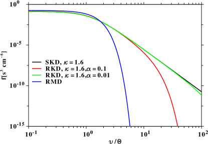
Figure 1: Comparison of the SKD (black line, for $n=1$ cm^-3, $\kappa=1.6$), RKD for $\alpha=0.1$ (red line) and $\alpha=0.05$ (green line), and the RMD for $\kappa\to\infty$ and $\alpha=1$ (blue line). While the abscissa corresponds to the normalized speed $x=v/\Theta$, the ordinate is in units of particles per phase space volume.

3 The regularized $\kappa$-distribution

Guided by the properties of the MD we introduce the regularized $\kappa$-distribution (RKD):

$$f(\kappa,\alpha,\Theta,v) \equiv \frac{N_{r\kappa}}{nN_{M}N_{\kappa}}f_{\kappa}(\Theta,v)f_{M}(\alpha,\Theta,v)$$

$$=nN_{r\kappa}\left(1+\frac{v^{2}}{\kappa\Theta^{2}}\right)^{-\kappa-1}\exp\left\{-\frac{\alpha^{2}v^{2}}{\Theta^{2}}\right\}$$

$$=nN_{r\kappa}\ {}_{1}F_{0}\left([\kappa+1],[];-\frac{v^{2}}{\kappa\Theta^{2}}\right)\exp\left\{-\frac{\alpha^{2}{v}^{2}}{{\Theta}^{2}}\right\}$$

where $f_{M}(w,v)=f_{M}(\alpha,\Theta,v)$ is provided by Eq. 2 for $w=\Theta/\alpha$, ${}_{1}F$ is a hypergeometric function (see appendix) and the normalisation constant $N_{r\kappa}=N_{r\kappa}(\alpha,\Theta)$ is given explicitly below. Obviously, the RKD has a power-law behaviour at low and intermediate speeds, and an exponential cut-off at higher speeds, regulated by the cut-off parameter $\alpha$.

3.1 Limits of the regularized $\kappa$-distribution

It is convenient to introduce a dimensionless argument $x=v/\Theta$ so that

$$f(\kappa,\alpha,\Theta,x) = nN_{r\kappa}\left(1+{x^{2}}/{\kappa}\right)^{-\kappa-1}\exp\left\{-\alpha^{2}x^{2}\right\}$$ (4)

$$=nN_{r\kappa}\ {}_{1}F_{0}\left([\kappa+1],[];-{x^{2}}/{\kappa}\right)\exp\left\{-{\alpha^{2}{x}^{2}}\right\}$$

Fig. 1 illustrates the differences between the RMD, SKD and the RKD (for two values of the cut-off parameter, $\alpha=0.1$, and 0.05. For low (normalised) speeds, i.e. $x<1/\alpha$, the deviations from the SKD are small, while for $x>1/\alpha$ the exponential function cuts off the SKD. In the limit of $x\gg\kappa$ the RKD can be approximated by

$$f(\kappa,\alpha,\Theta,x)\approx nN_{r\kappa}\kappa^{\kappa+1}x^{-2(\kappa+1)}\exp\left\{-\alpha^{2}x^{2}\right\}$$ (5)

Second, in the $\alpha\to 0$ the SKD is recovered, and, third, in the limit $\kappa\rightarrow\infty$ the RKD corresponds to a Maxwellian distribution of the form

$$\lim\limits_{\kappa\rightarrow\infty}f(\kappa,\alpha,\Theta,v)=nN_{r\infty}\exp\left\{-(1+\alpha^{2})\frac{v^{2}}{\Theta^{2}}\right\},$$ (6)

which is defined as in Eq.(2) with the choice $w=\Theta/\sqrt{1+\alpha^{2}}$, and the RMD is obtained for $\alpha\to 0$.

3.2 Properties of the regularized $\kappa$-distribution

1. For a given data set exhibiting a power-law behaviour, fits to measurements will yield the same results for the SKD and the RKD, if $\alpha$ can be chosen sufficiently small so that the cut-off occurs well beyond the range of observations. This is most often the case because most instruments take measurements within a finite velocity/speed interval. The fact that such results are insensitive to the use of the SKD or the RKD is illustrated below at the example of Langmuir waves.

2. The RKD is well-defined for all positive $\kappa$, i.e. resolves the divergence of the second-order moment of SKD, occurring for $\kappa\leqslant 3/2$.

3. Most importantly, all velocity moments of the RKD are finite (as shown in the next section), allowing to employ the RKD as a valid basis for a complete hydrodynamical description of a $\kappa$-distributed plasma.

3.3 Moments of the regularized $\kappa$-distribution

The isotropic velocity moments $M_{l}$ with $l\in\{0,1,2,...\}$ of the RKD are defined as

$$M_{l}(\kappa,\alpha,\Theta) = \int v^{l}f(\kappa,\alpha,\Theta,v)\mathrm{d}^{3}v$$

$$= 4\pi\int\limits_{0}^{\infty}v^{\nu}f(\kappa,\alpha,\Theta,v)dv$$

$$\equiv nN_{r\kappa}I(\kappa,\alpha,\nu,\Theta)$$

where $\nu=l+2$, and $4\pi$ and $v^{2}$ are additional factors resulting from the integration in spherical coordinates. The analytical solution of the integral $I(\kappa,\alpha,\nu,\Theta)$ and, thus, for all moments is given by

$$I(\kappa,\alpha,\nu,\Theta)= 4\pi\,\Theta^{1+{\nu}}\Bigg{\{}$$ (8)

$$-C_{1}\frac{\Gamma\left(a\right)\Gamma\left(b_{1}\right)}{4\Gamma\left(\kappa+1\right)}\mbox{${}_{1}$F${}_{1}$}(a;\,-b_{0};\,\alpha^{2}\kappa)$$

$$-C_{2}\frac{\Gamma\left(a\right)\Gamma\left(b_{2}\right)}{8\Gamma\left(\kappa+1\right)}\mbox{${}_{1}$F${}_{1}$}(a;\,-b_{1};\,\alpha^{2}\kappa)$$

$$+C_{3}\frac{1}{2}\Gamma\left(-b_{3}\right)\mbox{${}_{1}$F${}_{1}$}(\kappa;b_{4};\,\alpha^{2}\kappa)$$

$$-C_{4}\frac{1}{4}\Gamma\left(-b_{4}\right){\mbox{${}_{1}$F${}_{1}$}(\kappa;\,b_{5};\,\alpha^{2}\kappa)}\Bigg{\}}$$

with

$$a = \frac{\nu-1}{2},\qquad b_{i}=\frac{2\kappa-\nu+(2i-5)}{2}$$

$$\mathrm{and}$$

$$C_{1} = \alpha^{2}\left(2\alpha^{2}\kappa+\nu-1\right)\left(2-\kappa\right)\kappa^{\frac{\nu+3}{2}}$$

$$C_{2} = \left(4\alpha^{4}\kappa^{2}+\left[(4\nu-4)\alpha^{2}-2\nu+2\right]k+\nu^{2}-1\right)\kappa^{\frac{\nu+1}{2}}$$

$$C_{3} = \kappa^{\kappa+1}\alpha^{1+2\kappa-\nu}(\alpha^{2}+1)$$

$$C_{4} = (\nu-3)\kappa^{\kappa+1}\alpha^{3+2\kappa-\nu}$$

Formula (8) is the central result of the paper, as it allows to calculate all velocity moments of the RKD associated with a SKD. Further contrasting to the SKD, which is applicable only for $\kappa>3/2$, the RKD is defined for all $\kappa>0$, and all moments remain finite for any positive $\kappa>0$ and $\alpha>0$. ₁F₁ is the confluent hypergeometric function or Kummer function (see appendix).

The explicit form of the normalization constant $N_{r\kappa}$ can be provided by observing that $n=M_{0}(\kappa,\alpha,\Theta)$, so that

$$N_{r\kappa}=\frac{1}{I(\kappa,\alpha,2,\Theta)}$$ (9)

which in the case $\alpha=0$ reduces to $N_{\kappa}$, see Eq.(1), and for $\kappa\rightarrow\infty$ to $N_{M}$, see Eq.(2).

3.4 Velocity normalization and temperature definition

The two Maxwellian limits discussed in sec. II suggest two alternatives for interpreting an SKD. The first, claiming use of a $\kappa$-independent $\Theta$ (thermal speed), implies a $\kappa$-dependent temperature $T_{\kappa}=T_{\kappa}(\kappa)$ and admits the RMD limit for $\kappa\to\infty$ [15, 16, 14]. The second option is to assume a $\kappa$-independent temperature, which is usually convenient in computations. While there might be systems constrained to evolve under conditions of constant temperature [17], the more relevant case appears to be the former one [14, 11]. Also for the RKD the first choice is appropriate since the exponential cut-off should be independent of $\kappa$, implying that $\Theta$ cannot depend on $\kappa$. Consequently, the RKD is defined with a $\kappa$-dependent temperature, as follows. For a Maxwellian-distributed plasma one can define the temperature by

$$T_{M}=\frac{mP_{M}}{k_{B}n}$$ (10)

with $P_{M}$ being the second-order moment of the Maxwellian distribution function, which is the pressure (per mass unit) or the energy density.

We define the temperature of the RKD analogously:

$$T_{r\kappa} \equiv T_{r\kappa}(\kappa,\alpha,\Theta)\equiv\frac{mP_{r\kappa}}{nk_{B}}$$

$$= m\frac{N_{r\kappa}}{k_{B}}I(\kappa,\alpha,4,\Theta)=\frac{m}{k_{B}}\,\frac{I(\kappa,\alpha,4,\Theta)}{I(\kappa,\alpha,2,\Theta)}$$

The integral $I(\kappa,\alpha,2,\Theta)$ in the denominator is the same defining the normalization factor $N_{r\kappa}$ in Eq. 9, and the RKD pressure $P_{r\kappa}$ reads

$$P_{r\kappa}=n\frac{I(\kappa,\alpha,4,\Theta)}{I(\kappa,\alpha,2,\Theta)}.$$ (12)

The temperature $T_{r\kappa}$ as a function of $\Theta$, $\kappa$ and $\alpha$ is more complicated than $T_{\kappa}$ and $T_{M}$, and these are contrasted in Fig. 2. The RKD has continuously finite temperature values below $\kappa=3/2$ ( upper panel, Fig. 2), while the SKD temperature is not defined in that range. Moreover, for moderately high values of $\kappa$ (lower panel) like the ones reported by the observations in the solar wind [4], e.g., $2\leqslant\kappa\leqslant 6$ (far enough from the unphysical pole at $\kappa=3/2$) the temperature of RKD and SKD converge. For even higher values of $\kappa\to\infty$ the SKD and the RKD approach the Maxwellian limit. In the lower panel the blue line is the temperature of RKD for $\kappa=2$ and it is almost identical with that of SKD if $\alpha$ is sufficiently small, i.e., $\alpha<0.01$. For lower values of $\alpha$ the lines (blue, red, black) diverge when $\kappa$ decreases, while for higher values of $\alpha\rightarrow 1$ they converge to the RMD temperature. Thus, Fig. 2 illustrates why the RKD is a regularizing generalization of the SKD. While the SKD yields diverging temperature for $\kappa\leqslant 3/2$ and, thus, overestimates the temperature for $\kappa$-values approaching this pole, the RKD keeps the temperature at finite values for all $\kappa>0$. Furthermore, for the same $\kappa$-values indicated by the observations ($\kappa\gg 3/2$) and a sufficiently low parameter $\alpha$, the deviations of the RKD from the SKD are always small.

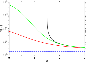
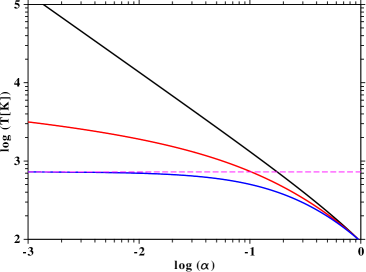
Figure 2: Upper panel: The temperature as a function of $\kappa$ as defined in Eq. 3.4 for $\Theta=1$ km/s, and $\alpha=0.1$ (red line) and $\alpha=0.01$ (green line), by comparison with the SKD temperature (black line) with its pole at $\kappa=3/2$ (black dashed vertical line), and the RMD temperature (dashed blue line). Lower panel: Variation of the temperature with $\alpha$. The black, red and blue lines correspond to $\kappa=1,1.5,2$, respectively. The dashed magenta (horizontal) line is the SKD temperature for $\kappa=2$.

4 Motivation for an exponential cut-off

Pure power law distributions in the particle velocity (or the momentum or the energy) are often observed in the context of acceleration processes. Such power laws are not well-posed for use over the whole velocity interval ($[0,\infty]$ in the classical or $[0,c]$ in the relativistic case, with $c$ the speed of light): in the limit $v\to 0$ the distributions diverge and in the limits $v\to\infty$ or $v\to c$ they correspond to diverging moments or unphysical boundary behaviour, respectively. While the SKD does not have the first defect, it is hampered by the second. Obviously, the existence of all velocity moments requires an exponential cut-off.

In the field of origin of $\kappa$-distributions, i.e. space physics, there are various cases of such exponential cut-offs of power laws. Particularly eloquent are the electron spectra, e.g., Figure 6 in [18], with evidences of two or three components (core, halo and superhalo) and each of them suggesting an exponential cutoff. We discuss two examples that also reveal the smallness of the cut-off parameter $\alpha$.

4.1 Acceleration in the interplanetary medium

Fisk & Gloeckler[19] have developed a theory based on rarefaction and compression waves in the solar wind in order to explain the frequently observed so-called $v^{-5}$-distributions of suprathermal particles. Their derivation resulted in distribution functions of the form

$$f_{FG}=f_{0,th}\left({v}/{v_{th}}\right)^{-5}\exp\left\{-{9D}/{((1+\beta)^{2}\delta u^{2}t})\right\},\;\;\;$$ (13)

i.e. power laws with an exponential cut-off. In the above formula $D=D_{0}v^{1+\beta}$ is the spatial diffusion coefficient, $v_{th}\approx 30$ km/s is the thermal speed, $\delta u^{2}$ quantifies fluctuations in velocity, and $t$ is time. This form corresponds to the limit discussed in Eq. 5 above, i.e. it is an RKD in the limit $v>\kappa\Theta$.

Assuming $\beta=1$ to obtain the standard $v^{2}$ dependence of $D$ and with the velocity diffusion coefficient $D_{vv}=\delta u^{2}v^{2}/(9D)$ we find

$$\frac{9D}{4\delta u^{2}t}=\frac{9Dv^{2}}{4\delta u^{2}tv^{2}}=\frac{v^{2}}{4D_{vv}t}=\frac{v^{2}}{4v_{typ}^{2}}=\alpha^{2}\frac{v^{2}}{\Theta^{2}},$$ (14)

where $v_{typ}$ is a typical speed, assumed to be a multiple of $\Theta$ and $\alpha={\Theta^{2}}/{4v_{typ}^{2}}=(4m^{2})^{-1}$, with an integer $m$. Hence, $\alpha$ is indeed a small parameter less than unity.

4.2 Acceleration at the solar wind termination shock

Steenberg & Moraal[20] used a distribution function of the type

$$f\propto\left({E_{kin}}/{E_{c}}\right)^{-q}\exp\left\{-b\left({E_{kin}}/{E_{c}}\right)^{2a}\right\}$$ (15)

to model the anomalous cosmic ray flux at the solar wind termination shock. Here $E_{kin}$ is the kinetic and $E_{c}$ a cut-off energy, with $q>0$. The authors did fit this expression to data and determined the parameters $a,b$ to be of the order of unity and 0.2, respectively. Thus, Eq.(15 resembles again an RKD with an $\alpha<1$.

5 On the persistence of kinetic results

In order to illustrate the influence on the results that are derived within the framework of kinetic theory, we consider (electrostatic) Langmuir waves. When using the RKD, these waves have the dispersion relation

$$0=1-{\omega_{pe}^{2}\over k^{2}\theta^{2}}Z^{\prime}_{\kappa,m}(\xi),\;\;{\rm where}\;\;\xi={\omega\over k\theta},$$ (16)

and $Z^{r}_{r,\kappa}(\xi)=\partial Z_{r,\kappa}(\xi)/\partial\xi$ is the derivative of what we can call the regularized $\kappa$-dispersion function

$$Z_{r,\kappa}(\xi)={1\over\kappa^{1/2}I_{0}}{1\over\pi^{1/2}}\int_{-\infty}^{\infty}{du\over u-\xi}\;{\exp\{-\alpha^{2}u^{2}\}\over\left(1+u^{2}/\kappa\right)^{\kappa}},$$ (17)

with

$$I_{0} = {\Gamma(\kappa-1/2)\over\Gamma(\kappa)}\,\mbox{${}_{1}$F${}_{1}$}\left({1\over 2},{3\over 2}-\kappa;\kappa\alpha^{2}\right)$$

$$+{\Gamma(1/2-\kappa)\over\pi^{1/2}}(\kappa\alpha^{2})^{\kappa-1/2}\,\mbox{${}_{1}$F${}_{1}$}\left(\kappa,\kappa+{1\over 2};\kappa\alpha^{2}\right).$$

For the derivative the explicit form reads

$$Z^{\prime}_{r,\kappa}(\xi)=-2\left\{\alpha^{2}+{I\over I_{0}}+\xi\left[\alpha^{2}Z_{r,\kappa}(\xi)+Z_{r,\kappa+1}(\xi)\right]\right\}$$ (19)

where

$$I = {\Gamma(\kappa+1/2)\over\Gamma(\kappa+1)}\,\mbox{${}_{1}$F${}_{1}$}\left({1\over 2},{1\over 2}-\kappa;\kappa\alpha^{2}\right)$$

$$-{\Gamma(1/2-\kappa)\over\pi^{1/2}(1/2+\kappa)}(\kappa\alpha^{2})^{\kappa+1/2}$$

$$\hskip 56.9055pt{}_{1}F_{1}\left(\kappa+1,\kappa+{3\over 2};\kappa\alpha^{2}\right),$$

and use was made of the identity $\Gamma(-1/2-\kappa)=-\Gamma(1/2-\kappa)/(1/2+\kappa)$. Fig. 3 displays the wave-number dispersion curves of the (normalised) frequencies $\omega_{r}(k)=\Re(\omega)(k)$ and damping rates $\gamma(k)=\Im(\omega)(k)$ for the SKD with $\alpha=0$ and two RKDs with $\alpha=0.1$ and $0.01$.

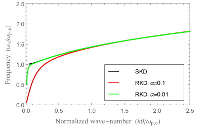
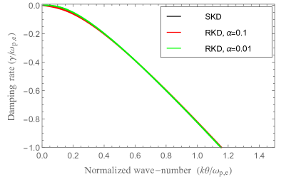
Figure 3: Langmuir modes dispersion curves $\omega_{r}(k)$ (left) and damping rates $\gamma(k)$ (right) for the SKD and the RKD.

Evidently, the RKD gives mostly the same values as the SKD, the differences being limited to low wave-numbers and decrease with decreasing cut-off parameter $\alpha$.

6 Conclusion

We defined a regularized $\kappa$-distribution (RKD) that, by contrast to the standard $\kappa$-distribution (SKD), has non-diverging velocity moments and is well-defined for all positive $\kappa$. Not only does the RKD remove all singularities from the theory of the SKD but it also allows to calculate all velocity moments analytically. The exponential cut-off of the RKD is motivated from theoretical considerations and from measurements. Both allow to determine the cut-off parameter to be significantly lower than unity. With such small values, fits to distributions of data are not sensitive to whether an SKD or an RKD is used, because the cut-off can be introduced beyond the observational threshold (of a given instrument).

Perspectives are now opened by a RKD to approach the plasma micro-states for low $\kappa$-values (i.e., below the limit $\kappa\leqslant 3/2$ imposed for a SKD), which have been excluded from the observational reports by reason of unrealistic parameter results [21] so far, although there is recently some indication of low-$\kappa$ power laws[22]. For higher $\kappa>3/2$ kinetic effects remain easily accessible by a SKD, while a macroscopic (fluid-like) description requires switching to the RKD. The moments of the SKD and the RKD differ significantly, so that any result obtained within a fluid approach must be expected to depend on this choice [23]. In practice, only the RKD allows a well-defined fluid approach, because only the RKD admits a complete (infinite) set of velocity moments that are well-defined for all positive $\kappa$-values.

Appendix

For convenience the two used generalized hypergeometric series (or functions) ${}_{1}F_{0}([a],[];x)$ and ${}_{1}F_{1}([],[b];x)$ are given here

$${}_{1}F_{0}([a],[];z) = \sum\limits_{n=0}^{\infty}(a)_{n}\,\frac{z^{n}}{n!}$$

$${}_{1}F_{1}([a],[b];z) = \sum\limits_{n=0}^{\infty}\frac{(a)_{n}}{(b)_{n}}\,\frac{z^{n}}{n!}$$

with $a,b\in\mathbb{R}\mathrm{\ and\ }z\in\mathbb{C}$, where $b\notin\{0,-1,...,-m\},$ $\ m\in\mathbb{N}$ and $(\bullet)_{n}$ is the Pochhammer symbol defined as

$$(a)_{0}=1$$

$$(a)_{n}=a(a+1)(a+2)...(a+n-1)\qquad n>0,n\in\mathbb{N}$$

Another notation for the confluent hypergeometric function ${}_{1}F_{1}([a],[b];z)$ is the Kummer function $M(a,b;x)$. For more details see [24] or [25].

References

- [1] Olbert S 1968 Summary of Experimental Results from M.I.T. Detector on IMP-1 Physics of the Magnetosphere (Astrophysics and Space Science Library vol 10) ed Carovillano R D L and McClay J F p 641
- [2] Vasyliunas V M 1968 J. Geophys. Res. 73 2839–2884
- [3] Treumann R A and Jaroschek C H 2008 Physical Review Letters 100 155005 (Preprint 0711.1676)
- [4] Pierrard V and Lazar M 2010 Sol. Phys. 267 153–174 (Preprint 1003.3532)
- [5] Beck C and Cohen E 2017 Chapter 6: Superstatistics: Superposition of maxwell–-boltzmann distributions Kappa Distributions ed Livadiotis G (Elsevier) pp 313 – 328 ISBN 978-0-12-804638-8 URL https://www.sciencedirect.com/science/article/pii/B9780128046388000061
- [6] Webb S, Litvinenko V N and Wang G 2012 Phys. Rev. STAB 15 080701 (Preprint 1105.0412)
- [7] Elkamash I S and Kourakis I 2016 Phys. Rev. E 94 053202
- [8] Student = Gosset, WS 1908 Biometrika 6 1–25 ISSN 0006-3444 (print), 1464-3510 (electronic) URL http://www.jstor.org/stable/2331554
- [9] Pearson, K 1916 Philosophical Transactions of the Royal Society of London A: Mathematical, Physical and Engineering Sciences 216 429–457 ISSN 0264-3952 (Preprint http://rsta.royalsocietypublishing.org/content/216/538-548/429.full.pdf) URL http://rsta.royalsocietypublishing.org/content/216/538-548/429
- [10] Abdul R F and Mace R L 2014 Comp. Phys. Comm. 185 2383–2386
- [11] Lazar M, Fichtner H and Yoon P H 2016 Astron. Astrophys. 589 A39 (Preprint 1602.04132)
- [12] Ziebell L F and Gaelzer R 2017 Phys. Plas. 24 102108
- [13] Lazar M, Pierrard V, Shaaban S M, Fichtner H and Poedts S 2017 Astron. Astrophys. 602 A44 (Preprint 1703.01459)
- [14] Lazar M, Poedts S and Fichtner H 2015 AA 582 A124
- [15] Leubner M P 2000 Planet. Space Sci. 48 133–141
- [16] Langmayr D, Biernat H K and Erkaev N V 2005 Physics of Plasmas 12 102103
- [17] Yoon P H 2014 Journal of Geophysical Research (Space Physics) 119 7074–7087
- [18] Lin R P 1998 Space Sci. Rev. 86 61–78
- [19] Fisk L A and Gloeckler G 2012 Space Sci. Rev. 173 433–458
- [20] Steenberg C D and Moraal H 1999 J. Geophys. Res. 104 24879–24884
- [21] ŠtveráK Š, Trávníček P, Maksimovic M, Marsch E, Fazakerley A N and Scime E E 2008 Journal of Geophysical Research (Space Physics) 113 A03103
- [22] Desai M I, Mason G M, Dayeh M A, Ebert R W, McComas D J, Li G, Cohen C M S, Mewaldt R A, Schwadron N A and Smith C W 2016 Astrophys. J. 828 106 (Preprint 1605.03922)
- [23] Fahr H J, Fichtner H and Scherer K 2014 J. Geophys. Res. 119 7998–8005
- [24] Abramowitz M and Stegun I A 1972 Handbook of Mathematical Functions (New York: Dover, 1972)
- [25] Gradshteyn I S and Ryzhik I M 2007 Table of integrals, series, and products (Elsevier/Academic Press, Amsterdam) ISBN 978-0-12-373637-6; 0-12-373637-4