A cost effective and reliable environment monitoring system for HPC applications

Abstract

We present a slow control system to gather all relevant environment information necessary to effectively and reliably run an HPC (High Performance Computing) system at a high value over price ratio. The scalable and reliable overall concept is presented as well as a newly developed hardware device for sensor read out. This device incorporates a Raspberry Pi, an Arduino and PoE (Power over Ethernet) functionality in a compact form factor. The system is in use at the 2 PFLOPS cluster of the Johannes Gutenberg-University and Helmholtz-Institute in Mainz.

url]https://him.uni-mainz.de/scientific-computing

1 Introduction

HPC systems are typically expensive large-scale devices in research. Consequently, monitoring is desirable for securing data and values (hardware). Furthermore, such environment monitoring also enables the optimization of operating parameters to increase efficiency (equivalent of minimizing the Power Usage Effectiveness, PUE) and thus a reduction of the carbon dioxide footprint.

In the HPC environment, hundreds of data points are collected usually at geographically widely scattered locations within several venues. The typical readout rate is in the order of about 1 Hz.

During the development phase, we aimed for a very high degree of reliability while at the same time simplifying the process of installation and operation. In addition, the use of widely used open source components (Raspberry Pi, Arduino) increases familiarity with the system components, i.e. enables fast installation, low cost of solution roll out and good debugging possibilities. The overall system can be crucial for operating any HPC system efficiently and safely.

Our environment monitoring system setup currently reads temperatures of water and air, humidity levels, water flow meters and water leakage sensors. The data is sent to a data collecting server running Ganglia [1] which enables time series monitoring as well as notifications in case of alarming conditions.

The problem of monitoring environmental data is not restricted to computing centers, where a lot of, in most parts redundant, effort is put into the solution of problems of this kind at various sites, both using commercial and custom made products. This work aims at documenting an all, i.e. including hardware design, open source solution to measuring and processing environmental data, which is flexible enough to incorporate various sensors while still being easy to implement.

2 Design

2.1 Overview

Our System consists of the following main elements: sensors, sensor aggregation unit (SAU) and a data collecting server – see the overview image 1.

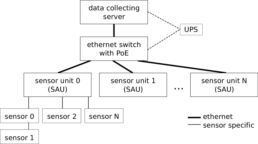
Figure 1: Overview of overall setup

Further necessary parts are a Power over Ethernet (PoE, IEEE 802.3af) enabled fast Ethernet switch (100 Mbit/s) as well as a single uninterruptible power supply (UPS) to overcome power outages or discontinuities. Due to the PoE enabled SAUs, the complete monitoring system down to the smallest sensor is UPS protected. In addition, careful selection of the Ethernet switch adds the functionality to remotely power cycle every sensor and sensor aggregation units out of the box.

2.2 Monitoring Network

Environmental sensors are connected to the sensor aggregation unit, get read out and send via an Ethernet link to the central collecting server. While the radius of Ethernet is specified for up to 100 meters, the sensor radius connected to a single SAU is limited to about 10 meters due to the usage of inexpensive RJ12 connectors, Y splitters and standard telephone cables. In a real environment, both limitations are negligible. As a side effect, the RJ12 ensures that no RJ45 network cable from the remaining HPC system gets plugged into the sensor network by mistake. The communication over the telephone cables are sensor specific and reach from static analog voltages to digital bus systems (at frequencies below 1 MHz).

2.3 Sensor Aggregation Unit

A sensor aggregation unit (SAU) consists of a mainboard and a Raspberry Pi as an add-on (see Fig. 2).

Figure 2: Sensor Aggregation Unit (SAU) and sensor cables

The mainboard provides the PoE functionality (IEEE 802.3af), an Arduino (Atmel ATMega 328PB) and bus driver (OneWire and I2C) functionality. The connection between the Arduino and the Raspberry Pi is done via its 40pin connector. Outgoing connections are only provided by the mainboard, these are the PoE enabled network connector and eleven RJ12 sensor ports. In total, these design decisions make the installation very compact and handy.

The decision to introduce an Arduino and to not connect the sensors directly to the Raspberry Pi was made for reasons of reliability and flexibility (due to program dependent pin usage). A serial connection together with a reset line links the Arduino with the Raspberry Pi. The reset line enables not only a reset of the Arduino but also in-system flashing. To enable this functionality, the optiboot bootloader has been preloaded via the ISP port on the mainboard. According to the design of the mainboard (16 MHz external low power crystal) low and high fuse bits have been set to 0xde [4].

Furthermore tests revealed an unstable behavior for a setup of four DS18B20 directly connected to the pins of a Raspberry Pi 2B with the latest (March 2017) Raspbian software release. To resolve these problems, the Raspberry Pi had to be power cycled because a simple reboot was not sufficient.

To further strengthen reliability the 5V line (generated by the PoE sub-module) powering the Raspberry Pi is not accessible from outside the sensor aggregation unit. Only the 3.3V derived by a low-dropout regulator (LDO) from it is available at the sensor connectors. Shortcuts on one of the sensor connectors will only affect the Arduino part, but will not bring the Raspberry Pi into an unstable state. As soon as the shortcut is resolved, the activated Brown-out Detection (BOD) (extended fuse bits = 0xfd) of the ATMega helps recovering immediately to a save state of operation.

Further benefits of the ATMega chip are its realtime capability and analog inputs to read out even more diverse sensors compared to the Raspberry Pi only solution.

The pin assignment of a RJ12 sensor port is listed in Tab. 1. They all share a common I2C bus (with optional internal 2.2 $\text{k}\Omega$ pull-ups, according to [5]) and have two additional I/O ports. One of it is enabled to act as an OneWire master, by activating the individual internal 4.7 $\text{k}\Omega$ pull-up. The second provides an analog I/O port for ports 1-6 and digital I/O for the remaining ports to read out an even larger selection of different sensor types.

Pin #	Description
1	3.3 VCC
2	Analog I/O (ports 1-6) or Digital I/O (ports 7-11)
3	Digital I/O (with optional individual pull-up for OneWire data)
4	I2C data (common for all ports, optional pull-up)
5	GND
6	I2C clock (common for all ports, optional pull-up)

Table 1: Pin assignment for the RJ12 sensor ports

The sensor aggregation unit schematics and the PCB layout are shown in Fig. 3.

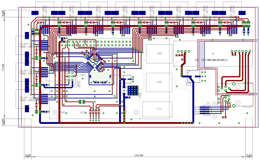
Figure 3: Electronics Layout

2.4 Sensors Recommendations

Among several sensors tested, the following were selected and are used in our setup. They fulfill a reasonable mix of performance and stability in comparison to their price:

• air / water temperature: Maxim DS18B20, sealed in stainless steel pipe, connection type: OneWire, response time: in still air $\tau\approx 90\text{\thinspace sec}$, accuracy $\Delta T=\pm 0.5\thinspace\text{K}$ [10]

• air temperature and humidity: IST HYT-271, connection type: I2C, response time: in still air $\tau\approx 180\text{\thinspace sec}$, with air-flow $\tau\approx 4\text{\thinspace sec}$, accuracy $\Delta T=\pm 0.2\thinspace\text{K}$ [11]

• water flow: water meter with reed contact as binary input

• air pressure: Bosch BME280 (together with temperature and humidity), connection type: I2C, response time: in still air $\tau\approx 270\text{\thinspace sec}$, with air-flow $\tau\approx 1\text{\thinspace sec}$, accuracy $\Delta T=\pm 1.0\thinspace\text{K}$ [12]

Some remarks for two of the above sensors: First, we custom ordered the OneWire temperature sensor from Maxim in a water-resistant packaging and a RJ12 connector matching our pin assignment and cable length. This makes installation as an air or water temperature sensor quick and easy. To increase the absolute precision of the sensor, we calibrated the offset individually before installation at 20 °C, see the result for 502 sensors in Fig. 4. This recalibration is done in the same units as the sensor outputs its data: degree Celsius.

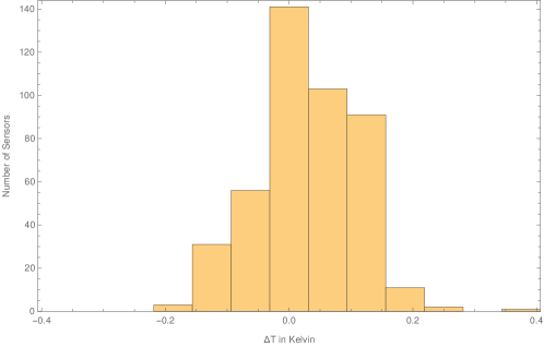
Figure 4: Miscalibration of 502 DS18B20 sensors at 20 °C. [13]

Secondly, the Bosch BME280 needs in general a recalibration over the complete temperature range. With the given individual sensor calibration constants, the temperature values do have a miscalibration in the order of $\pm 1\thinspace\text{K}$ (compare Tab. 2). This calibration fault increases further due to self heating and can be reduced when putting the sensor extensively into sleep mode. As a follow-up error, the temperature readings affect the humidity and pressure values. After recalibration, temperature readings operate reasonably stable (better than 0.1 K deviation over the complete range).

In the following, we describe the recalibration in a few steps: The sensor of interest is put together with a precise reference into a climate chamber and is exposed to temperatures between -40 °C and 60°C. The temperature is ramped up and down with less then 0.2 °C/min to allow for assimilation.

The data sheet [12] suggests a quadratic polynomial to calculate the real temperature $T$ [°C] with the measured raw-value $T_{\text{raw}}$

$$T=c_{0}+c_{1}T_{\text{raw}}+c_{2}T_{\text{raw}}^{2}$$

and

$$c_{0} = -\frac{4}{5\cdot 2^{22}}\left(d_{1}d_{2}-\frac{d_{1}^{2}d_{3}}{2^{16}}\right)$$

$$c_{1} = \frac{4}{5\cdot 2^{26}}\left(d_{2}-\frac{d_{1}d_{3}}{2^{15}}\right)$$

$$c_{2} = \frac{4}{5\cdot 2^{46}}d_{3}$$

where the constants $d_{i}$ have been calibrated in the factory according to the device. Fitting the measured data and choosing the positive solution provides a new set of high precision constants:

$$d_{1} = -\frac{c_{1}+\sqrt{c_{1}^{2}-4c_{0}c_{2}}}{32c_{2}}$$

$$d_{2} = \frac{5\cdot 2^{26}}{4}\sqrt{c_{1}^{2}-4c_{0}c_{2}}$$

$$d_{3} = \frac{5\cdot 2^{46}}{4}c_{2}$$

Example values for four sensors, before and after recalibration are given in Tab. 2.

sensor	factory calibration			new calibration			deviation
	$d_{1}$	$d_{2}$	$d_{3}$	$d_{1}$	$d_{2}$	$d_{3}$	-40..60 °C
1	28205	28205	50	28469	26034	753.63	-0.6 .. -1.8
2	28498	26766	50	30462	23501	2846.84	-2 .. -14
3	28222	26702	50	28172	26073	-388.33	1.2 .. -1.3
4	28266	26340	50	28304	26409	299.61	-0.3 .. 0.0

Table 2: Recalibration of BME280 sensors, $d_{1}$ is dimensionless, $d_{2}$ and $d_{3}$ are in °C.

2.5 Cabling and its Limitations

In this paragraph, we want to shortly describe some best practice hints for the sensor connecting cables as well as its limitations. Generally speaking, the maximum cable length and its network topology strongly depends on the electrical characteristics of the cables, passive distributor panels, number of sensors and bus type. To simplify the setup, we restricted our OneWire bus to a maximum radius of 10 Meter and not more than 15 sensors as we identified that problems occurred with our cabling hardware at about a 50 m radius. There is an interesting feature of the OneWire bus, which helps to easily determine the maximum length of the OneWire without any further instrumentation [2]: the most demanding operation of an OneWire bus is the device discovery procedure. Therefore if for some sensors the discovery does not reliably work, the capacity of the cable network is in the critical region and the length should be reduced (reduce number of sensors, cables or distributors). Even though a normal sensor readout does still work as it produces a lighter load on the network. A more sophisticated method is to determine the recovery time of the OneWire Bus [3] either with a software implementation on the Arduino (“pulsein” function) or with an oscilloscope. To comply with the standards, it should be well above 50 $\mu\text{s}$, when using not more than 15 sensors at room temperature.

3 Software

Although having the full flexibility of an open hardware design, the software on both the micro controller and collecting server is easy to deploy. Firstly, because it can be written as a widely-known Arduino program [6] and secondly, the Arduino program can be flashed online via the Raspberry Pi [7].

3.1 Microprocessor Programming

Due to the broad range of possible sensors, the program of the Arduino depends strongly on their choice. In the following, we describe the general structure of the firmware in our setup. After powering on a sensor the initialization procedure is started. From that point on, with a frequency of 1 Hz the information of all sensors is collected and handed over to the Raspberry Pi. The complete selection of software used on the Arduino is available online at [6].

3.2 Computer Programs Recommendation for reliable Usage

In our setup, we are using the Ganglia system [2] for the monitoring of the SAUs and for data collection. Another possibility is the use of EPICS [14] for that purpose, which has been deployed at another site. Both solutions are capable of collecting a number of data points in the order of $10^{3}$ on a single computer, i.e. their visualization and a historical charting functionality. The data collection server constantly monitors the SAUs and ensures the full sensor network is in a reliable state. Otherwise it will issue a software reset on the sensor device or performs a power cycle via the PoE functionality of the switch.

References

- [1] Ganglia distributed monitoring system for HPC, http://ganglia.sourceforge.net
- [2] Overview of 1-Wire Technology and Its Use, https://www.maximintegrated.com/en/app-notes/index.mvp/id/1796
- [3] Guidelines for Reliable Long Line 1-Wire Networks, https://www.maximintegrated.com/en/app-notes/index.mvp/id/148
- [4] Determining the Recovery Time for Multiple-Slave 1-Wire® Networks, https://www.maximintegrated.com/en/app-notes/index.mvp/id/3829
- [5] Atmel, ATmega328P, Datasheet complete http://www.atmel.com/Images/Atmel-42735-8-bit-AVR-Microcontroller-ATmega328-328P_Datasheet.pdf
- [6] Source code for SAU, https://github.com/peterotte/HPCSlowControl
- [7] Using avrdude with the Raspberry Pi, https://github.com/SpellFoundry/avrdude-rpi
- [8] I2C-bus specification and user manual, NXP http://www.nxp.com/docs/en/user-guide/UM10204.pdf
- [9] Example code and Schematics https://github.com/peterotte/HPCSlowControl
- [10] 1-Wire Digital Thermometer, DS18B20, Maxim Integrated, https://datasheets.maximintegrated.com/en/ds/DS18B20.pdf
- [11] Digital Humidity and Temperature Module, HYT 271, IST AG, https://www.ist-ag.com/sites/default/files/DHHYT271_E.pdf
- [12] Bosch Sensortec, BME280, Combined humidity and pressure sensor, final data sheet, document release date: 26/10/2015, https://www.bosch-sensortec.com/bst/products/all_products/bme280
- [13] Noskov, Dr. Sergey, Private Communication, 2018
- [14] EPICS, distributed soft real-time control systems, https://epics.anl.gov