Improved Runtime Bounds for the Univariate Marginal Distribution Algorithm via Anti-Concentration

Abstract

Unlike traditional evolutionary algorithms which produce offspring via genetic operators, Estimation of Distribution Algorithms (EDAs) sample solutions from probabilistic models which are learned from selected individuals. It is hoped that EDAs may improve optimisation performance on epistatic fitness landscapes by learning variable interactions. However, hardly any rigorous results are available to support claims about the performance of EDAs, even for fitness functions without epistasis. The expected runtime of the Univariate Marginal Distribution Algorithm (UMDA) on OneMax was recently shown to be in $\mathcal{O}\left(n\lambda\log\lambda\right)$ [8]. Later, Krejca and Witt [15] proved the lower bound $\Omega\left(\lambda\sqrt{n}+n\log n\right)$ via an involved drift analysis .

We prove a $O\left(n\lambda\right)$ bound, given some restrictions on the population size. This implies the tight bound $\Theta\left(n\log n\right)$ when $\lambda=O\left(\log n\right)$, matching the runtime of classical EAs. Our analysis uses the level-based theorem and anti-concentration properties of the Poisson-binomial distribution. We expect that these generic methods will facilitate further analysis of EDAs.

Index terms— Runtime Analysis, Level-based Analysis, Estimation of Distribution Algorithms

1 Introduction

Estimation of Distribution Algorithms are a class of randomised search heuristics with many practical applications [13]. Unlike traditional EAs which look for optimal solutions by explicitly building and maintaining a population of promising individuals, EDAs rely on a probabilistic model to represent information gained from the optimisation process over generations. There are many different variants of EDAs have been developed over the last decades, and the fundamental differences between them are the ways the interactions of decision variables are captured as well as how the probabilistic model is updated over generations. The earliest EDAs treated each variable independently, whereas later ones model variable dependencies [18]. Some examples of univariate EDAs are the compact genetic algorithm (cGA) and the Univariate Marginal Distribution Algorithm (UMDA). Multi-variate EDAs, such as the Bayesian Optimisation Algorithms which builds a Bayesian network with nodes and edges representing variables and conditional dependencies, attempt to learn relationships between the decision variables [13]. See [13] for other variants and more practical applications of EDAs.

The compact genetic algorithm was the first univariate EDA whose runtime was analysed rigorously. Introduced in [12], the algorithm samples two individuals in each generation and then evaluates them to determine the winner which is used to update the probabilistic model. A quantity of $1/K$ is shifted towards the winning bit value for each position where the two individuals differ. The first rigorous runtime analysis of cGA was completed by Droste in [9] where a lower bound $\Omega(K\sqrt{n})$ for any functions is provided using additive drift theory where $n$ being the problem size. The result is obtained by estimating an upper bound for an entity named surplus which is believed to reduce the overall running time if a large value appears in every generation. In addition, he proved an upper bound $\mathcal{O}(nK)$ for any linear function where $K=n^{1+\epsilon}$ for any small constant $\varepsilon>0$. Later studies showed that given a fitness function $f$, cGA have problems optimising functions with many $f$-independent bit positions, such as LeadingOnes [11]. This is because the marginal probabilities of those positions are very close to the borders 0 or 1, which makes it harder to change those bits. A variant of the cGA, the so-called stable compact genetic algorithm (scGA) was introduced where the marginal probability $p_{t}(i)$ of any $f$-independent position tends to concentrate around $1/2$ (i.e. stable). Given certain parameter settings, scGA is able to optimise LeadingOnes within $\mathcal{O}(n\log n)$ generations with probability polynomially close to $1$.

Similar to cGA, UMDA is a powerful algorithm with a wide range of applications not only in computer science but also in other areas. The most studied variant is often implemented with upper and lower borders for marginal probabilities to prevent decision variables from being fixed at values zero or one. The population in each generation is sampled from a joint distribution which is the product of marginal probabilities for all variables. The UMDA is related to the notion of linkage equilibrium, which is a popular assumption in Population Genetics. Hence, understanding of UMDA can contribute to the understanding of population dynamics in Population Genetics models.

Despite the fact that the UMDA has been analysed over the past years, the understanding of its runtime is still limited. The algorithm was analysed in series of papers [3, 5, 4, 6] where time-complexities of the UMDA on simple unimodal functions were derived. These result shows that UMDA with margins often outperforms other variants of UMDA without margins, especially on functions like BVLeadingOnes. Shapiro [18] investigated UMDA with a different selection mechanism rather than truncation selection. In particular, their variant of UMDA samples individuals whose fitnesses are no less than the mean fitness before using them to update the probabilistic model. By representing UMDA as a Markov chain, the paper shows that the population size has to be in the order of square-root of the problem size for UMDA to be able to optimise OneMax. The first upper bound on the expected optimisation time of UMDA on OneMax was not published until 2015 [8]. By working on another variant of UMDA which employs truncation selection, Dang and Lehre [8] proved an upper bound $\mathcal{O}(n\lambda\log\lambda)$ for UMDA on OneMax which requires a population size $\Omega(\log n)$. If $\lambda=\mathcal{O}(\log n)$, then the upper bound is $\mathcal{O}(n\log n\log\log n)$. The result is obtained by applying a relatively new technique called level-based theorem [7]. Very recently, Krejca and Witt [15] obtain a lower bound $\Omega(\mu\sqrt{n}+n\log n)$ of UMDA on OneMax via an involved drift analysis where $\lambda=(1+\Theta(1))\mu$. As can be seen, the upper and lower bounds are still different by $\Theta(\log\log n)$, which raises the question of whether this gap could be closed and a better asymptotic runtime would then be obtained.

This paper derives the upper bound $\mathcal{O}(n\lambda)$ for UMDA on OneMax which holds for $\lambda=\Omega(\mu)$ and $c\log n\leq\mu=\mathcal{O}(\sqrt{n})$ , where $c$ is some positive constant. If $\lambda=\mathcal{O}(\log n)$, we have a tight bound $\Theta(n\log n)$ which matches with the well-known expected runtime $\Theta(n\log n)$ of the (1+1) EA on the class of linear functions. The result is achieved with the application of an anti-concentration bound which might be of general interest. The new result improves the known upper bound $\mathcal{O}(n\lambda\log\lambda)$ of UMDA on OneMax [8] by removing the logarithmic factor $\mathcal{O}(\log\lambda)$. This improvement is significant becauses it for the first time it closes the gap mentioned above for a small range of population size. In addition, we also believe that the easy-to-use method employed to obtain the result can be used for other algorithms and fitness functions.

This paper is structured as follows. In Section $2$, we first present the UMDA algorithm under investigation. This section also includes a pseudo-code of the UMDA. The level-based theorem which is central in the paper will be stated in Section $3$. In this section, a sharp bound on the sum of Bernoulli random variables is also described. Given all necessary tools, Section $4$ illustrates our proof idea in a visual way and suggests how it could be applied for other problems. The main result for UMDA on OneMax is presented in Section $5$. Section $6$ presents a brief empirical analysis of UMDA on OneMax to complement the theoretical findings in Section $5$. Finally, concluding remarks are given in Section $7$.

Independent work: Witt [19] independently obtained the upper bounds $\mathcal{O}(\mu n)$ on the expected optimisation time of the UMDA on OneMax for $\mu\geq c\log n$, where $c$ is a positive constant, and $\lambda=(1+\Theta(1))\mu$ using an involved drift analysis. While our result does not hold for $\mu=\omega(\sqrt{n})$, our methods yield a significantly easier proof which also holds when the parent population size $\mu$ is not proportional to the offspring population size $\lambda$.

2 UMDA

The Univariate Marginal Distribution Algorithm (UMDA) proposed in [17] is one of the simplest variants of Estimation of Distribution Algorithms. In each generation, the algorithm builds a probabilistic model over the search space based on information gained about the individuals in the previous generation. To optimise a pseudo-Boolean fitness function $f:\{0,1\}^{n}\rightarrow\mathbb{R}$, the UMDA builds a product distribution represented by a vector $p_{t}=\left(p_{t}(1),p_{t}(2),\ldots,p_{t}(n)\right)$ in every generation $t\in\mathbb{N}$. Each component $p_{t}(i)\in[0,1]$ for $i\in[n]$ and $t\in\mathbb{N}$ represents the probability of sampling a 1-bit at the $i$-th position of the offspring in generation $t+1$ where $[n]$ denotes the set $\{1,2,3,\ldots,n\}$. Therefore, each candidate solution $(x_{1},\ldots,x_{n})\in\{0,1\}^{n}$ is sampled with joint probability

$$\Pr\left(x_{1},\ldots,x_{n}\right)=\prod_{i=1}^{n}p_{t}(i)^{x_{i}}\cdot(1-p_{t}(i))^{(1-x_{i})}.$$

We will use the standard initialisation $p_{0}(i)\coloneqq 1/2$ for all $i\in[n]$. Starting with the initial model $p_{0}$, the algorithm continuously, in every generation $t\in\mathbb{N}$, sample $\lambda$ individuals $P_{t}(1),\ldots,P_{t}(\lambda)$ using the current model $p_{t}$. All individuals in the current population are sorted according to their fitnesses, and the top $\mu$ individuals are selected to compute the next model $p_{t+1}$. Let $P_{t}(k,i)$ denote the value in the $i$-th bit position of the $k$-th individual in current population $P_{t}$. Then each component of the next model is defined as

$$p_{t+1}(i)\coloneqq\frac{1}{\mu}\sum_{k=1}^{\mu}P_{t}(k,i)$$

which can be interpreted as the frequency of 1-bit among the $\mu$ best individuals in position $i$.

The special case $p_{t+1}(i)\in\{0,1\}$ must be avoided because the bit in position $i$ would remain fixed forever at either 0 or 1. This would result in parts of the search space becoming unreachable. In order to prevent this situation, the model components are often restricted to a closed interval, i.e. $p_{t+1}(i)\in[m^{\prime}/\mu,1-m^{\prime}/\mu]$, where the parameter $m^{\prime}<\mu$ controls the size of the margins. For completeness, the following pseudo-code describes the full algorithm (see Algorithm 1).

begin

       initialise $p_{0}(i)=1/2$ for all $i\in[n]$,

       for $t=0,1,2,\ldots$ until termination condition met do

             for $k=1,2,\ldots,\lambda$ do

                   sample $P_{t}(k,i)\sim\operatorname{Ber}\left(p_{t}(i)\right)$ for all $i\in[n]$

                  

            sort $P_{t}$ in descending order according to fitness,

             for $i=1,2,\ldots,n$ do

                   let $X_{i}\coloneqq\sum_{k=1}^{\mu}P_{t}(k,i),$

                   if $X_{i}<m^{\prime}$ then

                        $p_{t+1}(i)=m^{\prime}/\mu$,

                   else if $X_{i}>\mu-m^{\prime}$ then

                         $p_{t+1}(i)=1-m^{\prime}/\mu$,

                   else

                        $p_{t+1}(i)=X_{i}/\mu$.

                  

            

      

Algorithm 1 UMDA

3 Methods

3.1 Level-Based Theorem

The level-based theorem is a general tool that provides upper bounds on the expected optimisation time of many population-based algorithms on a wide range of optimisation problems. For example, it has been successfully applied to investigate the runtime of the Genetic Algorithms with or without crossover on various problems like Linear or LeadingOnes [7]. Besides, the first upper bounds of UMDA on OneMax and LeadingOnes have been obtained using this method [8].

The theorem assumes that the algorithm to be analysed can be described in the form of Algorithm 2. Let $\mathcal{X}$ be a finite search space which is, for example, $\{0,1\}^{n}$ in the case of binary representation. The algorithm considers a population $P_{t}$ at generation $t\in\mathbb{N}$ of $\lambda$ individuals that is represented as a vector $(P_{t}(1),P_{t}(2),\ldots,P_{t}(\lambda))\in\mathcal{X}^{\lambda}$. The theorem is general because it does not assume specific fitness functions, selection mechanisms, or generic operators like mutation and crossover. Rather, the theorem assumes that there exists, possibly implicitly, a mapping $\mathcal{D}$ from the set of populations $\mathcal{X}^{\lambda}$ to the space of probability distribution over the search space $\mathcal{X}$. The mapping $\mathcal{D}$ depends only on the current population and is used to produce the individuals in the next generation [7].

Data: Finite search space $\mathcal{X}$, population size $\lambda\in\mathbb{N}$, a

mapping $\mathcal{D}$ from $\mathcal{X}^{\lambda}$ to probability distributions over $\mathcal{X}$, and an initial population $P_{0}\in\mathcal{X}^{\lambda}.$

begin

       for $t=0,1,2,\ldots$ until termination condition met do

             for $i=1,2,3,\ldots,\lambda$ do

                   sample $P_{t+1}(i)\sim\mathcal{D}(P_{t})$

            

      

Algorithm 2 Population-based algorithm

Furthermore, the theorem assumes a partition $A_{1},\ldots,A_{m}$ of the search space $\mathcal{X}$ into $m$ subsets, which we call levels. We assume that the last level $A_{m}$ consists of all optimal solutions. Although there are many different ways to create the partition, it should be chosen using prior knowledge of the specific problem under investigation and the behaviour of the algorithm. One class of such partition is the well-known canonical fitness-based partition where all solutions with the same $f$-value are gathered to form a level. Let $A_{\geq j}\coloneqq\cup_{i=j}^{m}A_{i}$ be the set of all individuals belonging to level $A_{j}$ or higher. We denote $|P_{t}\cap A_{j}|\coloneqq|\{i\mid P_{t}(i)\in A_{j}\}|$ to be the number of individuals of the population $P_{t}$ belonging to level $A_{j}$. Given these conventions, we can state the level-based theorem as follows.

Theorem 1 (Theorem 1, [7]).

Given a partition $\left(A_{i}\right)_{i\in[m]}$ of $\mathcal{X}$, define $T\coloneqq\min\{t\lambda\mid|P_{t}\cap A_{m}|>0\}$ to be the first time $t$ that at least one element of level $A_{m}$ appears in the current population $P_{t}$. If there exist $z_{1},\ldots,z_{m-1},\delta\in(0,1]$, and $\gamma_{0}\in(0,1)$ such that for any population $P_{t}\in\mathcal{X}^{\lambda}$,

• (G1) for each level $j\in[m-1]$, if $|P_{t}\cap A_{\geq j}|\geq\gamma_{0}\lambda$ then

  $$\Pr_{y\sim\mathcal{D}(P_{t})}\left(y\in A_{\geq j+1}\right)\geq z_{j}.$$

• (G2) for each level $j\in[m-2]$, and all $\gamma\in(0,\gamma_{0}]$, if $|P_{t}\cap A_{\geq j}|\geq\gamma_{0}\lambda$ and $|P_{t}\cap A_{\geq j+1}|\geq\gamma\lambda$ then

  $$\Pr_{y\sim\mathcal{D}(P_{t})}\left(y\in A_{\geq j+1}\right)\geq\left(1+\delta\right)\gamma.$$

• (G3) and the population size $\lambda\in\mathbb{N}$ satisfies

  $$\lambda\geq\left(\frac{4}{\gamma_{0}\delta^{2}}\right)\ln\left(\frac{128m}{z_{*}\delta^{2}}\right)$$

  where $z_{*}\coloneqq\min_{j\in[m-1]}\{z_{j}\}$, then

  $$\mathbb{E}\left[T\right]\leq\left(\frac{8}{\delta^{2}}\right)\sum_{j=1}^{m-1}\left[\lambda\ln\left(\frac{6\delta\lambda}{4+z_{j}\delta\lambda}\right)+\frac{1}{z_{j}}\right].$$

Informally, the first condition (G1) requires that the probability to obtain an individual at level $A_{j+1}$ or higher is at least $z_{j}$ given that at least $\gamma_{0}\lambda$ individuals in the current population are in level $A_{j}$ or higher. Condition (G2) requires that given that $\gamma_{0}\lambda$ individuals of the current population belong to level $A_{j}$ or higher, and, moreover, $\gamma\lambda$ of them are lying at levels no lower than $A_{j+1}$, the probability of sampling a new offspring belonging to level $A_{j+1}$ or higher is no smaller than $(1+\delta)\gamma$. The last condition (G3) sets a lower limit on the population size $\lambda$. As long as all three conditions are satisfied, an upper bound on the expected runtime of the population-based algorithm is guaranteed.

Traditionally in Evolutionary Computation, we often define running time (or optimisation time) as the total number of fitness evaluations performed by the algorithm until an optimal solution has been found for the first time. However, the random variable $T\coloneqq\min\{t\lambda\mid|P_{t}\cap A_{m}|>0\}$ in Theorem 1 is the total number of candidate solutions sampled by the algorithm until the first generation where an optimal solution is witnessed for the first time. In the context of UMDA, these two entities are not always identical as $T$ is never smaller than the optimisation time. Since the level-based theorem provides upper bounds on the optimisation time, this will not cause any problems.

The detailed proof of the level-based theorem can be seen in [7] in which drift theory is applied to the distance measured by a level function. To apply the level-based theorem, it is recommended to follow a five-step procedure (see [7] for more details). It starts by identifying a proper partition of the search space, and then find specific parameter settings such that conditions (G1) and (G2) are met, followed by verifying that the population size that should be large enough, and, finally, an upper bound on the expected runtime is provided.

3.2 A Uniform Bound on the Sum of Bernoulli Trials

In order to show that conditions (G1) and (G2) in the level-based theorem are verified, we will use a sharp upper bound on the probability $\Pr\left(Y=y\right)$ for any $y$, where $Y$ represents the level of a sampled offspring. Let $Y_{i}$ be a Bernoulli random variable with success probability $p_{i}$ that represents the bit value at position $i$ in a sampled offspring, and then $Y\coloneqq\sum_{i=1}^{n}Y_{i}$. The distribution of $Y$ is known as the Poisson-Binomial Distribution, and it has expectation $\mathbb{E}\left[Y\right]=\sum_{i=1}^{n}p_{i}$ and variance $\sigma_{n}^{2}=\sum_{i=1}^{n}p_{i}\left(1-p_{i}\right)$. We will make use of a sharp upper bound on $\Pr\left(Y=y\right)$ from [1].

Theorem 2 (Theorem 2.1, [1]).

Let $Y_{1},Y_{2},\ldots,Y_{n}$ be $n$ independent Bernoulli random variables with success probability $p_{i}$. Let $Y=\sum_{i=1}^{n}Y_{i}$ denote the sum of these random variables and let $\sigma_{n}^{2}=\sum_{i=1}^{n}p_{i}(1-p_{i})$ be the variance of $S_{n}$. The following result holds for all $n$, $y$ and $p_{i}$

$$\sigma_{n}\cdot\Pr\left(Y=y\right)\leq\eta$$

where $\eta$ is an absolute constant being

$$\eta=\max_{\lambda\geq 0}\sqrt{2\lambda}e^{-2\lambda}\sum_{k=0}^{\infty}\left(\frac{\lambda^{k}}{k!}\right)^{2}\sim 0.4688.$$

3.3 Feige’s Inequality

To demonstrate that conditions (G1) and (G2) of the level-based theorem hold, it is necessary to compute lower bounds on the probability of $\Pr\left(Y\geq y\right)$ where $Y$ represents the level of a sampled individual. Following [8], we will make use of a general result due to Feige to compute such lower bounds [10] when $y<\mathbb{E}\left[Y\right]$. For our purposes, it will be convenient to use the following variant of Feige’s theorem.

Theorem 3 (Corollary 3, [8]).

Let $Y_{1},\dots,Y_{n}$ be $n$ independent random variables with support in $[0,1]$, define $Y=\sum_{i=1}^{n}Y_{i}$ and $\mu=\mathbb{E}\left[Y\right]$. It holds for every $\Delta>0$ that

$$\Pr\left(Y>\mu-\Delta\right)\geq\min\left\{\frac{1}{13},\frac{\Delta}{1+\Delta}\right\}.$$

4 Proof idea

This section is dedicated to showing how the upper bound on the expected runtime of UMDA on OneMax is achieved using the level-based theorem with anti-concentration bounds. Our approach refines the analysis in [8] by taking into account anti-concentration properties of the random variables involved. As already discussed in Section 3.1, we need to verify three conditions (G1), (G2) and (G3) before an upper bound is guaranteed. The first two conditions concern the probability of sampling an offspring belonging to a higher level. Often verifying condition (G2) requires less effort than that of condition (G1) since for (G2) we usually have more information on the current population by assumption.

We chose $m^{\prime}<1$, then it follows that the marginal probabilities are in

$$p_{t}(i)\in\left\{\frac{k}{\mu}\mid k\in[\mu-1]\right\}\cup\left\{1-\frac{1}{n},\frac{1}{n}\right\}.$$

When $p_{t}(i)=1-1/n$ or $1/n$, we say that the marginal probability is at the upper or lower border, respectively. Therefore, we can categorise values for $p_{t}(i)$ into three groups: those at the upper margin $1-1/n$, those at the lower margin $1/n$, and those within the closed interval $[1/\mu,1-1/\mu]$. For OneMax, all bits have the same weight and the fitness is just the sum of these bit values, so the re-arrangement of bit positions will not have any impact on the distribution of sampled offspring. As a result, without loss of generality, we can re-arrange the bit-positions so that for two integers $k,\ell\geq 0$, it holds

• for all $i\in[1,k],$ $1\leq X_{i}\leq\mu-1$ and $p_{t}(i)=X_{i}/\mu$,

• for all $i\in(k,k+\ell]$, $X_{i}=\mu$ and $p_{t}(i)=1-1/n$, and

• for all $i\in(k+\ell,n]$, $X_{i}=0$ and $p_{t}(i)=1/n$.

Given the search space $\mathcal{X}\coloneqq\{0,1\}^{n}$, we define the levels as the canonical fitness-based partition

$$A_{j} \coloneqq\left\{x\in\mathcal{X}\mid\text{\sc OneMax}(x)=j-1\right\}.$$ (1)

For a given time $t\in\mathbb{N}$, and for all integers $i,j$ with $1\leq i\leq j\leq n$, define the Poisson-Binomially distributed random variables

$$Y_{i,j}\coloneqq\sum_{k=i}^{j}Y_{k},\quad\text{ where }\quad Y_{k}\sim\operatorname{Ber}(p_{t}(k))\quad\text{ for all }k\in[n].$$

Note that the probability occurring in conditions (G1) and (G2) of the level-based theorem can now be re-written as

$$\Pr_{y\sim\mathcal{D}(P_{t})}\left(y\in A_{\geq j+1}\right)=\Pr\left(Y_{1,n}\geq j\right).$$

To verify condition (G1), by assumption all $\mu$ top candidate solutions in the current population belong to $A_{j}$, i.e. having exactly $j-1$ one-bits. We need to calculate a lower bound $z_{j}$ on the probability of sampling an offspring having at least $j$ 1-bits. This probability $\Pr(Y_{1,n}\geq j)$ is the area marked by the diagonal lines in Figure 1.

Figure 1: Distribution of number of one-bits

We aim to obtain an upper bound $\mathcal{O}(n\lambda)$ of UMDA on OneMax using the level-based theorem. Note that the logarithmic factor $\mathcal{O}(\log\lambda)$ in the first upper bound $\mathcal{O}(n\lambda\log\lambda)$ in [8] stems from the lower bound $z_{j}=\Omega(\mu^{-1})$. We need a better bound $z_{j}=\Omega\left((n-j+1)/n\right)$. This led us to consider three cases according to different configurations of the current population in Step 3 of Theorem 4 below.

1. $k\geq\mu$. We will see that this implies that the variance of $Y_{1,k}$ is quite large, hence the distribution of $Y_{1,k}$ cannot be too concentrated on the mean $\mathbb{E}[Y_{1,k}]=j-\ell-1$. As a result, it is sufficient to get an extra 1-bit from the first $k$ positions to obtain an offspring belonging to $A_{\geq j+1}$. The probability of sampling $j$ 1-bits is bounded from below by $\Pr(Y_{1,n}\geq j)\geq\Pr(Y_{1,k}\geq j-\ell)\cdot\Pr(Y_{k+1,k+\ell}=\ell)$, where $\Pr(Y_{1,k}\geq j-\ell)$ is measured using the anti-concentration result from Theorem 2 and Lemma 1.

2. $k<\mu$ and $j\geq n+1-n/\mu$. In this case, the current level is very close to the optimal one, and the bitstring has few zero-bits. As already obtained from [8], the upgrade probability in this case is $\Omega(\mu^{-1})$. Since the condition can be rewritten as $\mu^{-1}\geq(n-j+1)/n$, it ensures that $z_{j}=\Omega(\mu^{-1})=\Omega((n-j+1)/n)$.

3. The remaining cases. Later will we prove that given $\mu\leq\sqrt{n(1-c)}$ for some constant $c\in(0,1)$, all remaining cases excluded by the first two cases are covered in $0\leq k<(1-c)(n-j+1)$. In this case, $k$ is relatively small, and $\ell$ is not too large since the current level is not very close to the optimal one. This implies that most zero-bits must be located in the last $n-k-\ell$ positions, and it suffices to sample an extra 1-bit from this region. The probability of sampling an offspring belonging to levels $A_{\geq j+1}$ is then $\Omega((n-j+1)/n)$.

5 Runtime of UMDA on OneMax

OneMax is the problem of maximising the number of one-bits in a bitstring, and is formally defined by $\text{\sc OneMax}\left(x\right)=\sum_{i=1}^{n}x_{i}$. It is well-known that the OneMax problem can be optimised in expected time $\Theta(n\log n)$ using the $(1+1)$ Evolutionary Algorithm. The level-based theorem was applied to derive the first upper bound on the expected optimisation time of the UMDA on OneMax, which is $\mathcal{O}(n\lambda\log\lambda)$, assuming $\lambda=\Omega(\log n)$ [8]. By refining this method, we will obtain the better bound $\mathcal{O}(n\lambda)$.

Theorem 4.

For some constant $a>0$, and any constant $c\in(0,1)$, the UMDA with parent population size $a\ln(n)\leq\mu\leq\sqrt{n(1-c)}$, offspring population size $\lambda\geq(13e)\mu/(1-c)$, and margin $m^{\prime}\coloneqq\mu/n$, has expected optimisation time $\mathcal{O}\left(n\lambda\right)$ on OneMax.

Proof.

First, we define $\gamma_{0}\coloneqq\mu/\lambda$. Since $\mu\leq\sqrt{n(1-c)}$, it follows that $m^{\prime}=\mu/n<1$, and the upper and lower borders for $p_{t}(i)$ simplify to $1-1/n$ and $1/n$, respectively. We re-arrange the bit positions and define the random variable $Y_{i,j}$ as in Section 4. We now closely follow the recommended 5-step procedure for applying the level-based theorem [7].

Step 1. The levels are defined as in Eq. (1). There are exactly $m=n+1$ levels from $A_{1}$ to $A_{n+1}$, where level $A_{n+1}$ consists of the optimal solution.

Step 2. We verify condition (G2) of the level-based theorem. In particular, for some $\delta\in(0,1),$ and for any level $j\in[m-2]$, and any $\gamma\in(0,\gamma_{0}]$, assuming that the population is configured such that $|P_{t}\cap A_{\geq j}|\geq\gamma_{0}\lambda=\mu$ and $|P_{t}\cap A_{\geq j+1}|\geq\gamma\lambda>0$, we must show that the probability to sample an offspring belonging to level $A_{j+1}$ or higher must be no less than $(1+\delta)\gamma$. By the re-arrangement of the bit-positions mentioned in Section 4, it holds

$$\sum_{i=k+1}^{k+\ell}X_{i}=\mu\ell\quad\mbox{ and }\quad\sum_{i=k+\ell+1}^{n}X_{i}=0,$$ (2)

where $X_{i},i\in[n],$ are given in Algorithm 1. By assumption, the current population $P_{t}$ consists of at least $\gamma\lambda$ individuals with $j$ one-bits and $\mu-\gamma\lambda$ individuals with $j-1$ one-bits, therefore

$$\sum_{i=1}^{n}X_{i}\geq\gamma\lambda j+\left(\mu-\gamma\lambda\right)(j-1)=\gamma\lambda+\mu\left(j-1\right).$$ (3)

Combining (2), (3) and noting that $\lambda=\mu/\gamma_{0}$ yield

$$\sum_{i=1}^{k}X_{i} =\sum_{i=1}^{n}X_{i}-\sum_{i=k+1}^{k+\ell}X_{i}-\sum_{i=k+\ell+1}^{n}X_{i}$$

$$\geq\gamma\lambda+\mu\left(j-1\right)-\mu\ell=\mu\left(j-\ell-1+\frac{\gamma}{\gamma_{0}}\right).$$

Let $Z=Y_{1,k}+Y_{k+\ell+1,n}$ be the total number of 1-bits sampled in the first $k$ and the last $n-k-\ell$ positions. $Y_{1,k}$ and $Y_{k+\ell+1,n}$ take integer values only, and so does $Z$. Since $k+\ell\leq n$, the expected value of $Z$ is

$$\begin{split}\mathbb{E}\left[Z\right]&=\sum_{i=1}^{k}p_{t}(i)+\sum_{i=k+\ell+1}^{n}p_{t}(i)\\ &=\frac{1}{\mu}\left(\sum_{i=1}^{k}X_{i}\right)+\frac{1}{n}\left(n-k-\ell\right)\geq j-\ell-1+\frac{\gamma}{\gamma_{0}}.\end{split}$$

In order to obtain an offspring with at least $j$ one-bits, it is sufficient to sample $\ell$ one-bits in positions $k+1$ to $k+\ell$ and at least $j-\ell$ one-bits from the other positions. The probability of this event is bounded from below by

$$\Pr\left(Y_{1,n}\geq j\right)\geq\Pr\left(Z\geq j-\ell\right)\cdot\Pr\left(Y_{k+1,k+\ell}=\ell\right).$$ (4)

The probability to obtain $\ell$ 1-bits in the middle interval from position $k+1$ to $k+\ell$ is

$$\Pr\left(Y_{k+1,k+\ell}=\ell\right)=\left(1-\frac{1}{n}\right)^{\ell}\geq\left(1-\frac{1}{n}\right)^{n-1}\geq\frac{1}{e}.$$ (5)

We now need to calculate $\Pr\left(Z\geq j-\ell\right)$. Since $Z$ takes integer values only, then

$$\begin{split}\Pr\left(Z\geq j-\ell\right)&=\Pr\left(Z>j-\ell-1\right)\\ &\geq\Pr\left(Z>\mathbb{E}\left[Z\right]-\frac{\gamma}{\gamma_{0}}\right).\end{split}$$

Applying Theorem 3 for $\Delta=\gamma/\gamma_{0}\leq 1$ and noting that we chose $\mu$ and $\lambda$ such that such that $1/\gamma_{0}=\lambda/\mu\geq 13e/(1-c)=13e(1+\delta)$ yield

$$\Pr\left(Z\geq j-\ell\right) \geq\min\bigg{\{}\frac{1}{13},\frac{\Delta}{\Delta+1}\bigg{\}}$$ (6)

$$\geq\frac{\Delta}{13}=\frac{\gamma}{13\gamma_{0}}\geq e\left(1+\delta\right)\gamma.$$ (7)

Therefore, combining (4), (5), and (7) give $\Pr\left(Y_{1,n}\geq j\right)\geq\left(1+\delta\right)\gamma$, and condition (G2) holds.

Step 3. We now consider condition (G1) for any level $j$ defined with $\gamma=0$. In other words, all the top $\mu$ individuals in the current population $P_{t}$ have exactly $j-1$ one-bits, and, therefore, $\sum_{i=1}^{n}X_{i}=\mu\left(j-1\right)$ and $\sum_{i=1}^{k}X_{i}=\mu\left(j-\ell-1\right)$. There are three different cases that cover all situations according to variables $k$ and $j$.

Case 1: Assume that $k\geq\mu$. The variance of the first $k$ bits is

$$\operatorname{Var}\left[Y_{1,k}\right]=\sum_{i=1}^{k}p_{t}(i)\left(1-p_{t}(i)\right)\geq\frac{k}{\mu}\left(1-\frac{1}{\mu}\right)\geq\frac{9k}{10\mu}\geq\frac{9}{10},$$

where the second inequality holds for sufficiently large $n$ because $\mu\geq a\ln(n)$. Theorem 2 applied with $\sigma_{k}\geq\sqrt{9/10}$ now gives

$$\Pr\left(Y_{1,k}=j-\ell-1\right)\leq\eta/\sigma_{k}.$$

Furthermore, since $\mathbb{E}\left[Y_{1,k}\right]$ is an integer, Lemma 1 implies

$$\Pr\left(Y_{1,k}\geq\mathbb{E}\left[Y_{1,k}\right]\right)\geq 1/2.$$

By combining these two probability bounds, the probability to obtain at least $j-\ell$ one-bits from the first $k$ positions is

$$\Pr\left(Y_{1,k}\geq j-\ell\right) =\Pr\left(Y_{1,k}\geq j-\ell-1\right)-\Pr\left(Y_{1,k}=j-\ell-1\right)$$

$$=\Pr\left(Y_{1,k}\geq\mathbb{E}\left[Y_{1,k}\right]\right)-\Pr\left(Y_{1,k}=j-\ell-1\right)$$

$$\geq\frac{1}{2}-\frac{\eta}{\sigma_{k}}>\frac{1}{2}-\frac{0.4688}{\sqrt{9/10}}=\Omega(1).$$ (8)

In order to obtain an offspring belonging to levels $A_{\geq j+1}$, it is sufficient to sample at least $j-\ell$ one-bits from the first $k$ positions and $\ell$ 1-bits from position $k+1$ to position $k+\ell$. By (5) and (8), the probability of this event is bounded from below by

$$\Pr\left(Y_{1,n}\geq j\right) \geq\Pr\left(Y_{1,k}\geq j-\ell\right)\cdot\Pr\left(Y_{k+1,k+\ell}=\ell\right)$$

$$>\Omega(1)\cdot\frac{1}{e}=\Omega(1).$$

Case 2: $k<\mu$ and $j\geq n(1-1/\mu)+1$. The second condition is equivalent to $1/\mu\geq(n-j+1)/n$. The probability to obtain an offspring belonging to levels $A_{\geq j+1}$ is then bounded from below by

$$\Pr\left(Y_{1,n}\geq j\right)\geq\\ \Pr\left(Y_{1,1}=1\right)\Pr\left(Y_{2,k}\geq j-\ell-1\right)\Pr\left(Y_{k+1,k+\ell}=\ell\right)\\ \geq\frac{1}{\mu}\Pr\left(Y_{2,k}\geq j-\ell-1\right)\frac{1}{e}\geq\frac{1}{14e\mu},$$

where we used the inequality $\Pr\left(Y_{2,k}\geq j-\ell-1\right)\geq 1/14$ for $\mu\geq 14$ proved in [8]. Since $1/\mu\geq(n-j+1)/n$, we can conclude that

$$\Pr\left(Y_{1,n}\geq j\right)\geq\frac{1}{14e\mu}\geq\frac{n-j+1}{14en}=\Omega\left(\frac{n-j+1}{n}\right).$$

Case 3: $k<\mu$ and $j<n(1-1/\mu)+1$. This case covers all the remaining situations not included by the first two cases. The latter inequality can be rewritten as $n-j+1\geq n/\mu$. We also have $\mu\leq\sqrt{n(1-c)}$, so $n/\mu\geq\mu/(1-c)$, then

$$(1-c)(n-j+1)\geq(1-c)(n/\mu)\geq(1-c)\mu/(1-c)=\mu>k.$$

Thus, the two conditions can be shortened to $0\leq k<(1-c)(n-j+1)$. In this case, the probability of sampling $j$ one-bits is

$$\Pr(Y_{1,n}\geq j)$$

$$\geq\Pr\left(Y_{1,k}\geq j-\ell-1\right)\Pr\left(Y_{k+1,k+\ell}=\ell\right)\Pr\left(Y_{k+\ell+1,n}\geq 1\right)$$

$$\geq\frac{1}{2}\cdot\frac{1}{e}\cdot\frac{n-k-\ell}{n}=\frac{n-k-\ell}{2en}.$$

Since $\ell\leq j-1$ and $k<(1-c)(n-j+1)$, then

$$\Pr\left(Y_{1,n}\geq j\right)>\frac{n-(1-c)(n-j+1)-j+1}{2en}=\Omega\left(\frac{n-j+1}{n}\right).$$

Combining all three cases together yields the upgrade probability

$$\Pr\left(Y_{1,n}\geq j\right) \geq\min\bigg{\{}\Omega(1),\;\Omega\left(\frac{n-j+1}{n}\right)\bigg{\}}=\Omega\left(\frac{n-j+1}{n}\right)=:z_{j},$$

and, therefore, $z_{*}\coloneqq\min_{j\in[n]}\{z_{j}\}=\Omega(1/n)$.

Step 4. We consider condition (G3) regarding the population size. We have $1/\delta^{2}=\mathcal{O}(1)$, $1/z_{*}=\mathcal{O}(n)$, and $m=\mathcal{O}(n)$. Therefore there must exist a constant $a>0$ such that

$$\left(\frac{a}{\gamma_{0}}\right)\ln(n)\geq\left(\frac{4}{\gamma_{0}\delta^{2}}\right)\ln\left(\frac{128m}{z_{*}\delta^{2}}\right).$$

The requirement $\mu\geq a\ln(n)$ now implies that

$$\lambda=\frac{\mu}{\mu/\lambda}\geq\left(\frac{a}{\gamma_{0}}\right)\ln(n)\geq\left(\frac{4}{\gamma_{0}\delta^{2}}\right)\ln\left(\frac{128m}{z_{*}\delta^{2}}\right),$$

hence condition (G3) is satisfied.

Step 5. We have shown that conditions (G1), (G2), and (G3) are satisfied. By Theorem 1 and the bound $z_{j}=\Omega((n-j+1)/n)$, the expected optimisation time is therefore

$$\mathbb{E}\left[T\right]=\mathcal{O}\left(\lambda\sum_{j=1}^{n}\ln\left(\frac{n}{n-j+1}\right)+\sum_{j=1}^{n}\frac{n}{n-j+1}\right).$$

We now estimate the two terms separately. By Stirling’s approximation (Lemma 2), the first term is

$$\mathcal{O}\left(\lambda\sum_{j=1}^{n}\ln\left(\frac{n}{n-j+1}\right)\right) =\mathcal{O}\left(\lambda\ln\prod_{j=1}^{n}\frac{n}{n-j+1}\right)=\mathcal{O}\left(\lambda\ln\frac{n^{n}}{n!}\right)$$

$$=\mathcal{O}\left(\lambda\ln\frac{n^{n}\cdot e^{n}}{n^{n+1/2}}\right)=\mathcal{O}\left(n\lambda\right).$$

The second term is

$$\mathcal{O}\left(\sum_{j=1}^{n}\frac{n}{n-j+1}\right)=\mathcal{O}\left(n\sum_{k=1}^{n}\frac{1}{k}\right)=\mathcal{O}\left(n\log n\right).$$

Since $\lambda>\mu=\Omega(\log n)$, the expected optimisation time is

$$\mathbb{E}\left[T\right]=\mathcal{O}\left(n\lambda\right)+\mathcal{O}\left(n\log n\right)=\mathcal{O}\left(n\lambda\right).$$

∎

6 An empirical result

So far we have proven an upper bound $\mathcal{O}\left(n\lambda\right)$ on the expected runtime of UMDA on OneMax with parent population size $a\log n\leq\mu=\mathcal{O}(\sqrt{n})$ , offspring population size $\lambda=\Omega(\mu)$, and margin size $m^{\prime}\leq 1$. This result is tighter than the bound $\mathcal{O}(n\lambda\log\lambda)$, obtained in [8], which provided the first upper bound for UMDA on OneMax. However, the bound $\mathcal{O}(n\lambda)$ is asymptotic and only provides information on the growth of the expected runtime according to the problem size $n$ for sufficiently large $n\geq n_{0}$. It provides no information on the multiplicative constant or the influences of lower order terms. Hence it makes sense to consider the empirical runtime of UMDA on OneMax to partially compensate for the limitations in the theoretical analysis.

We carry out a small experiment by running the UMDA on OneMax with initial parameter settings consistent with those conditions mentioned above. The settings of parameters are as follows: $\lambda=\sqrt{n}$, $\mu=\log n$ and $m^{\prime}=0.5$ for $n\in\{100,200,\ldots,10000\}$. The results are shown in Figure 2. For each value of $n$, the algorithm is run 100 times, and then the average runtime is computed. The mean runtime for each value of $n$ is estimated with 95% confidence intervals using the bootstrap percentile method [16] with 100 bootstrap samples. Each mean point is plotted with two error bars to illustrate the upper and lower margins of the confidence intervals.

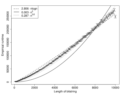
Figure 2: Mean runtime of UMDA on OneMax with 95% confidence intervals plotted with error bars. The fitted models are also plotted.

From the parameter settings chosen for the experiment, Theorem 4 gives the upper bound $\mathcal{O}(n^{3/2})$ for the expected optimisation time. We now compare this theoretical bound with the empirical runtime and two other bounds close to this model: $\mathcal{O}(n\log n)$ which is the runtime of (1+1) EA on OneMax, and the quadratic bound $\mathcal{O}(n^{2})$. Following [16], we fit three positive constants $c_{1},c_{2}$ and $c_{3}$ to the models $c_{1}\cdot n\log n$, $c_{2}\cdot n^{3/2}$ and $c_{3}\cdot n^{2}$ using non-linear least square regression. The correlation coefficient for each model is calculated to measure the fit of each model to the data.

Table 1: Best-fit models.

Best-fit function	Correlation coefficient
$2.806\cdot n\log n$	0.9994
$0.287\cdot n^{3/2}$	0.9900
$0.003\cdot n^{2}$	0.9689

From Table 1, it can be seen that the first two models $2.806\cdot n\log n$ and $0.287\cdot n^{3/2}$, with the correlation coefficients $0.9994$ and $0.9900$ respectively, fit well with the empirical data. The quadratic model fits less well with the empirical data. These findings are consistent with the theoretical expected optimisation time since the first two models are members of $\mathcal{O}(n^{3/2})$. As already stated before, our bound $\mathcal{O}(n\lambda)$ is tight for $\lambda=\mathcal{O}(\log n)$; however, in this experiment we chose a larger offspring population size $\lambda=\sqrt{n}$. For this case, the model $2.806\cdot n\log n$ has higher correlation coefficient than the model $0.287\cdot n^{3/2}$, indicating that our theoretical bound may not be tight for this case.

7 Conclusion

Despite the long-time use of EDAs by the Evolutionary Computation community, little has been known about their runtime, even for apparently simple settings such as UMDA on OneMax. Results about the UMDA are not only relevant to Evolutionary Computation, but also to Population Genetics where it corresponds to the notion of linkage equilibrium.

We have proved the upper bound $\mathcal{O}(n\lambda)$ which holds for $a\log n\leq\mu=\mathcal{O}(\sqrt{n})$ where $a$ is a positive constant. Although our result assumes that $\lambda\geq(1+c^{\prime})\mu$ for some positive constant $c^{\prime}>0$, it does not require that $\mu$ is proportional in size to $\lambda$. The bound is tight when $\lambda=\mathcal{O}(\log n)$; in this case, a tight bound $\Theta(n\log n)$ on the expected optimisation time of the UMDA on OneMax is obtained, matching the well-known bound $\Theta(n\log n)$ for the (1+1) EA on the class of linear functions. Although the bound assumes a not too large parent population size $\mu=\mathcal{O}(\sqrt{n})$, it finally closes the $\Theta(\log\log n)$ gap between the first upper bound $\mathcal{O}(n\log n\log\log n)$ [8] for certain settings of $\lambda$ and $\mu$ and the recently discovered lower bound $\Omega(\mu\sqrt{n}+n\log n)$ for $\lambda=(1+\Theta(1))\mu$ [15]. Future work should consider the runtime of UMDA on OneMax for larger offspring population sizes $\mu=\omega(\sqrt{n})$ and different combinations of $\mu$ and $\lambda$, as well as the runtime on more complex fitness landscapes.

Our analysis further demonstrates that the level-based theorem can yield, relatively easily, asymptotically tight bounds for non-trivial, population-based algorithms. An important additional component of the analysis was the use of anti-concentration properties of the Poisson-Binomial distribution. Unless the variance of the sampled individuals is not too small, the distribution of the population cannot be too concentrated anywhere, yielding sufficient diversity to discover better solutions. We expect that these arguments will lead to new results in runtime analysis of evolutionary algorithms.

We use the following property of the Poisson-Binomial distribution.

Lemma 1 (Theorem 3.2, [14]).

Let $Y_{1},Y_{2},\ldots,Y_{n}$ be $n$ independent Bernoulli random variables. Let $Y\coloneqq\sum_{i=1}^{n}Y_{i}$ be the sum of these random variables and let $\mu$ be the expectation of $Y$. If $\mu$ is an integer, then

$$\Pr\left(Y\geq\mu\right)\geq 1/2.$$

Lemma 2 (Stirling’s approximation [2]).

For all $n\in\mathbb{N}$,

$$n!=\Theta\left(\frac{n^{n+1/2}}{e^{n}}\right).$$

References

- [1] Jean-Bernard Baillon, Roberto Cominetti, and Jose Vaisman. 2016. A sharp uniform bound for the distribution of sums of Bernoulli trials. Combinatorics, Probability and Computing 25, 3 (2016), 352–361.
- [2] Ronald Rivest Charles E. Leiserson, Clifford Stein and Thomas H. Cormen. 2009. Introduction to Algorithms. MIT Press.
- [3] Tianshi Chen, Ke Tang, Guoliang Chen, and Xin Yao. 2007. On the analysis of average time complexity of estimation of distribution algorithms. In Proceedings of the IEEE Congress on Evolutionary Computation, CEC 2007. 453–460.
- [4] Tianshi Chen , Per Kristian Lehre , Ke Tang , Xin Yao, When is an estimation of distribution algorithm better than an evolutionary algorithm?, Proceedings of the Eleventh conference on Congress on Evolutionary Computation, p.1470-1477, May 18-21, 2009, Trondheim, Norway
- [5] Tianshi Chen , Ke Tang , Guoliang Chen , Xin Yao, Rigorous time complexity analysis of univariate marginal distribution algorithm with margins, Proceedings of the Eleventh conference on Congress on Evolutionary Computation, p.2157-2164, May 18-21, 2009, Trondheim, Norway
- [6] Tianshi Chen , Ke Tang , Guoliang Chen , Xin Yao, Analysis of computational time of simple estimation of distribution algorithms, IEEE Transactions on Evolutionary Computation, v.14 n.1, p.1-22, February 2010
- [7] D. Corus, D. C. Dang, A. V. Eremeev and P. K. Lehre, ”Level-Based Analysis of Genetic Algorithms and Other Search Processes,” in IEEE Transactions on Evolutionary Computation, vol. PP, no. 99, pp. 1-1. doi: 10.1109/TEVC.2017.2753538.
- [8] Duc-Cuong Dang and Per Kristian Lehre. 2015. Simplified Runtime Analysis of Estimation of Distribution Algorithms. In Proceedings of the 2015 Annual Conference on Genetic and Evolutionary Computation (GECCO ’15), Sara Silva (Ed.). ACM, New York, NY, USA, 513-518. DOI: http://dx.doi.org/10.1145/2739480.2754814.
- [9] Stefan Droste. 2006. A rigorous analysis of the compact genetic algorithm for linear functions. 5, 3 (September 2006), 257-283. DOI=http://dx.doi.org/10.1007/s11047-006-9001-0.
- [10] Uriel Feige. 2004. On sums of independent random variables with unbounded variance, and estimating the average degree in a graph. In Proceedings of the thirty-sixth annual ACM symposium on Theory of computing (STOC ’04). ACM, New York, NY, USA, 594-603. DOI: http://dx.doi.org/10.1145/1007352.1007443.
- [11] Tobias Friedrich, Timo Kötzing, and Martin S. Krejca. 2016. EDAs cannot be Balanced and Stable. In Proceedings of the Genetic and Evolutionary Computation Conference 2016 (GECCO ’16), Tobias Friedrich (Ed.). ACM, New York, NY, USA, 1139-1146. DOI: https://doi.org/10.1145/2908812.2908895.
- [12] G. R. Harik, F. G. Lobo and D. E. Goldberg, ”The compact genetic algorithm,” in IEEE Transactions on Evolutionary Computation, vol. 3, no. 4, pp. 287-297, Nov 1999. doi: 10.1109/4235.797971.
- [13] Mark Hauschild and Martin Pelikan. 2011. An introduction and survey of estimation of distribution algorithms. Swarm and Evolutionary Computation 1, 3 (2011), 111–128.
- [14] Kumar Jogdeo and S. M. Samuels. 1968. Monotone Convergence of Binomial Probabilities and a Generalization of Ramanujan’s Equation. The Annals of Mathematical Statistics 39, 4 (1968), 1191–1195.
- [15] Martin S. Krejca , Carsten Witt, Lower Bounds on the Run Time of the Univariate Marginal Distribution Algorithm on OneMax, Proceedings of the 14th ACM/SIGEVO Conference on Foundations of Genetic Algorithms, January 12-15, 2017, Copenhagen, Denmark.
- [16] Per Kristian Lehre , Xin Yao, Runtime analysis of the (1+1) EA on computing unique input output sequences, Information Sciences: an International Journal, 259, p.510-531, February, 2014.
- [17] Heinz Mühlenbein , Gerhard Paass, From Recombination of Genes to the Estimation of Distributions I. Binary Parameters, Proceedings of the 4th International Conference on Parallel Problem Solving from Nature, p.178-187, September 22-26, 1996.
- [18] J. L. Shapiro, Drift and Scaling in Estimation of Distribution Algorithms, Evolutionary Computation, v.13 n.1, p.99-123, January 2005.
- [19] Carsten Witt, Upper bounds on the runtime of the univariate marginal distribution algorithm on onemax, Proceedings of the Genetic and Evolutionary Computation Conference, July 15-19, 2017, Berlin, Germany.