Effect of partially ionized impurities and radiation on the effective critical electric field for runaway generation

Abstract

We derive a formula for the effective critical electric field for runaway generation and decay that accounts for the presence of partially ionized impurities in combination with synchrotron and bremsstrahlung radiation losses. We show that the effective critical field is drastically larger than the classical Connor–Hastie field, and even exceeds the value obtained by replacing the free electron density by the total electron density (including both free and bound electrons). Using a kinetic equation solver with an inductive electric field, we show that the runaway current decay after an impurity injection is expected to be linear in time and proportional to the effective critical electric field in highly inductive tokamak devices. This is relevant for the efficacy of mitigation strategies for runaway electrons since it reduces the required amount of injected impurities to achieve a certain current decay rate.

• (Dated: )

Keywords: runaway electron, tokamak, disruption, Fokker–Planck

1 Introduction

When a plasma carrying a large electric current is suddenly cooled, as happens in tokamak disruptions, a large toroidal electric field is induced due to the dramatic increase of the plasma resistivity. If this electric field is larger than a certain critical electric field, a relativistic runaway electron beam can be generated [1, 2]. Such runaway beams can damage the plasma facing components on impact due to localized energy deposition. Therefore, runaway electrons constitute a significant threat to large tokamak experiments (e.g. ITER) [3, 4, 5].

To minimize the risk of damage, it is crucial to understand the runaway-electron dynamics. Disruption mitigation by material injection is motivated by the strong influence of partially ionized atoms, as observed in experiments [3, 4, 6]. It is therefore important to have accurate models of the interaction between fast electrons and the partially screened nuclei of heavy ions. Fast electrons are not simply deflected by the Coulomb interaction with the net charge of the ion, but probe its internal electron structure, so that the nuclear charge is not completely screened. Energetic electrons can therefore be expected to experience higher collision rates against partially ionized impurities compared to a fully ionized plasma with the same effective charge, leading to a more efficient damping. There has been a considerable effort to produce a detailed theoretical description of this process [7, 8, 9, 10].

A recent paper presented a generalized collision operator which describes the interaction between fast electrons and partially screened impurities via analytic modifications to the collision frequencies [9]. The elastic electron-ion collisions were modeled quantum-mechanically in the Born approximation as in [7, 8], however, to obtain the required electron-density distribution of the impurity ions [7, 8] used the Thomas-Fermi model. In Ref. [9] we used fitted results from density functional theory (DFT) thereby providing a more accurate description. To describe inelastic collisions with bound electrons, we employed Bethe’s theory for the collisional stopping power [11], with mean ionization energies for ions calculated in [12]. Our results show that, already at sub-relativistic electron energies, the deflection and slowing-down frequencies are increased significantly compared to standard collisional theory [9].

The quantity that is arguably the most important for runaway generation and decay is the threshold, or critical, electric field, which in a fully ionized plasma without radiation losses is given by the Connor-Hastie field $E_{\rm c}\!=\!n_{\rm e}e^{3}\ln\Lambda/(4\pi\epsilon_{0}^{3}m_{\rm e}c^{2})$ [2], where $n_{\rm e}$ and $m_{\rm e}$ are the electron density and mass, $\ln\Lambda$ is the Coulomb logarithm, $\epsilon_{0}$ is the vacuum permittivity and $c$ is the speed of light. Below the threshold field no new runaway electrons are produced and all preexisting runaways eventually thermalize. There is a wealth of experimental evidence that the critical electric field is much higher than $E_{\rm c}$ given above [13, 14, 15, 16, 17, 18]. Well-diagnosed and reproducible experiments in quiescent plasmas on a wide range of tokamaks show that measured threshold electric fields can be approximately an order of magnitude higher than predicted by the Connor-Hastie threshold [13, 18]. Furthermore, it has been shown that the runaway electron current decays much faster after high-$Z$ particle injection than expected from conventional theory [2], in contrast to low-$Z$ particle injection which results in a current decay rate only slightly below that expected [14]. From a theoretical point of view, the threshold electric field is expected to be higher than $E_{\rm c}$, as can be influenced by synchrotron [19, 20] and bremsstrahlung radiation losses, and also, as we will show here, by the presence of partially ionized atoms. The value of the critical electric field is not only interesting theoretically – it is of immense practical importance as it determines the amount of material that has to be injected in disruption mitigation schemes [21].

In this paper we derive an analytical expression for the effective critical field for runaway generation and decay that takes into account the presence of partially screened impurities, using the generalized collision operator derived in [9]. We present a formula that accounts for arbitrary ion species in combination with synchrotron and bremsstrahlung losses. We show that the effect of partially screened impurities is captured by replacing the plasma density in the critical electric field with an effective density $n\!=\!n_{\rm free}\!+\!\kappa n_{\rm bound}$, where $\kappa$ is typically in the range 1-2 which implies that the effect of bound electrons is significantly larger than suggested by previous studies [22]. Furthermore, using a kinetic equation solver with a 0D inductive electric field, we verify the prediction from [21], that the runaway current in highly inductive tokamak devices after impurity injection will decay linearly with time at a rate proportional to the effective electric field. We expect these findings will facilitate future comparisons with experimental observations of runaway-current decay, however such analysis is beyond the scope of the present paper.

The structure of the paper is as follows. In section 2 we describe the kinetic model accounting for the effect of partial screening in both the generalized collision operator and the bremsstrahlung operator. Then we proceed in section 3 to derive analytical expressions for the effective critical electric field in the presence of partially ionized impurities. This calculation generalizes the results in [20], in which the critical electric field was calculated by assuming rapid pitch-angle dynamics in the Fokker–Planck equation. In contrast to [20], our study includes the effect of partially ionized impurities and bremsstrahlung losses. We demonstrate how the presence of partially screened impurities affects both synchrotron losses (through pitch-angle scattering) and bremsstrahlung (as partial screening affects the bremsstrahlung cross-section). In section 4 we discuss the decay of a runaway current when heavy impurities are injected. Through kinetic simulations, we demonstrate the accuracy of the analytical expressions for the effective critical electric field and the current decay. Finally in section 5 we summarize our conclusions.

2 Kinetic equation including partially screened impurities

In a uniform, magnetized plasma, the kinetic equation for relativistic electrons can be written as follows:

$$\frac{\partial f}{\partial\tau}+\underbrace{\frac{E}{E_{\rm c}}\!\left(\xi\frac{\partial f}{\partial p}+\frac{1\!-\!\xi^{2}}{p}\frac{\partial f}{\partial\xi}\right)}_{\rm electric\,field}$$

$$=\underbrace{\vphantom{\frac{\partial}{\partial p}}C_{\rm FP}\{f\}+S_{\rm ava}}_{\rm collisions}+\underbrace{C_{\rm br}\{f\}-\frac{\partial}{\partial\bi{p}}\!\cdot\!\left(\bi{F}_{\rm syn}f\right)}_{\rm radiation\,reaction}\,,$$ (1)

where $f$ is the electron distribution function, $C_{\rm FP}\{f\}$ is the partially screened Fokker–Planck collision operator as described in section 2.1, which accounts for ionizing as well as elastic collisions. The avalanche source is denoted $S_{\rm ava}$ and $E$ is the component of the electric field which is antiparallel to the magnetic field $\bi{B}$. Radiation losses are modeled by $C_{\rm br}$ (the bremsstrahlung collision operator) and $\bi{F}_{\rm syn}$ (the synchrotron radiation reaction force), which are described in section 2.2. The normalized momentum is defined as $p\!=\!\gamma v/c$ is (with $\gamma$ the Lorentz factor), $\xi=\bi{p}\cdot\bi{B}/(pB)$ is the cosine of the pitch-angle, and the time variable $\tau$ is normalized to the relativistic collision time

$$\tau_{\rm c}\!=\!4\pi\epsilon_{0}^{2}m_{\rm e}^{2}c^{3}/(n_{\rm e}e^{4}\ln\Lambda_{\rm c}),$$

where we introduced a relativistic Coulomb logarithm

$$\ln\Lambda_{\rm c}=\ln\Lambda_{0}+\frac{1}{2}\ln\frac{m_{\rm e}c^{2}}{T}\approx 14.6+0.5\ln(T_{\rm eV}/n_{e20}).$$ (2)

Here, $T_{\rm eV}$ is the temperature in $\rm eV$, $n_{e20}$ is normalized to $10^{20}\,\mathrm{m^{-3}}$ and $\ln\Lambda_{0}=14.9-0.5\ln n_{e20}+\ln T_{\rm keV}$ is the thermal electron-electron Coulomb logarithm [23]. The temperature dependence of $\ln\Lambda_{\rm c}$ is reduced compared to $\ln\Lambda_{0}$ as it describes collisions between thermal particles and relativistic electrons; (2) corresponds to evaluating the energy-dependent electron-ion Coulomb logarithm $\ln\Lambda^{\rm ee}$ at $\gamma=2$. For future reference, the superthermal Coulomb logarithms are given by [24]

$$\ln\Lambda^{\rm ee}=\ln\Lambda_{\rm c}+\ln\sqrt{(\gamma\!-\!1)}$$ (3)

and

$$\ln\Lambda^{\rm ei}=\ln\Lambda_{\rm c}+\ln(\sqrt{2}p)\,.$$ (4)

The parallel electric field $E$ is thus most naturally compared to the critical electric field $E_{\rm c}$ defined with the relativistic Coulomb logarithm $\ln\Lambda_{\rm c}$ (rather than the thermal $\ln\Lambda_{0}$):

$$E_{\rm c}=\frac{n_{\rm e}e^{3}\ln\Lambda_{\rm c}}{4\pi\epsilon_{0}^{2}m_{\rm e}c^{2}}=\frac{m_{\rm e}c}{e\tau_{\rm c}}.$$

2.1 Collision frequencies with partially ionized impurities

When acting on relativistic electrons and $T\ll m_{\rm e}c^{2}$, the linearized Fokker–Planck collision operator $C_{\rm FP}\{f\}$ can be simplified to

$$C_{\rm FP}\{f\}=\nu_{\rm D}\mathscr{L}\{f\}+\frac{1}{p^{2}}\frac{\partial}{\partial p}\left(p^{3}\!{\nu_{\rm s}}f\right),$$

where $\mathscr{L}=\frac{1}{2}\frac{\partial}{\partial\xi}\left(1-\xi^{2}\right)\frac{\partial}{\partial\xi}$ is the Lorentz scattering operator. The slowing-down frequency $\nu_{\rm s}=\nu_{\rm s}^{\rm ee}$ and the deflection frequency $\nu_{\rm D}=\nu_{\rm D}^{\rm ee}+\nu_{\rm D}^{\rm ei}$ are well known in the limits of complete screening (i.e. the electron interacts only with the net ion charge) and no screening (the electron experiences the full nuclear charge). The generalized expressions for $\nu_{\rm D}^{\rm ei}$ and $\nu_{\rm s}^{\rm ee}$ taking into account partial screening are given in [9].

Focusing on the effective critical electric field $E_{\rm c}^{\rm eff}$ in this paper, the following equations are specialized to the superthermal momentum region, in which the critical momentum $p_{\rm c}$ corresponding to $E_{\rm c}^{\rm eff}$ is found. Thus all of the following expressions are given for superthermal electrons.

The generalized deflection frequency is, in units of $\tau_{\rm c}^{-1}$, given by

$$\nu_{\rm D}=\frac{\gamma}{p^{3}}\bar{\nu}_{\rm D},$$

$$\bar{\nu}_{\rm D}=\frac{1}{\ln\Lambda_{\rm c}}\bigg{[}\ln\Lambda^{\rm ee}+\ln\Lambda^{\rm ei}Z_{\rm eff}$$

$$+\sum_{j}\frac{n_{j}}{n_{\rm e}}\left((Z_{j}^{2}\!-\!Z_{0,j}^{2})\ln\left(\bar{a}_{j}p\right)-\frac{2}{3}N_{{\rm e},j}^{2}\right)\bigg{]}.$$ (5)

Here, $Z_{0,j}$ is the ionization state, $Z_{j}$ is the charge number and $N_{{\rm e},j}=Z_{j}\!-\!Z_{0,j}$ is the number of bound electrons of the nucleus for species $j$, $Z_{\mathrm{eff}}=\sum_{j}n_{j}Z_{0,j}^{2}/n_{\rm e}$, where $n_{j}$ is the density of species $j$, and $n_{\rm e}$ represents the density of free electrons. The parameter $\bar{a}_{j}$ was determined from DFT calculations, and is an effective ion size which depends on the ion species $j$. These constants are given for argon and neon in table 1 in A. In (5), we have assumed $p\gg 1/\bar{a}_{j}\simeq 10^{-2}$. Figure 1a shows the enhancement of the deflection frequency for singly ionized argon and neon. At typical runaway energies in the MeV range, the enhancement is more than an order of magnitude compared to taking the limit of complete screening and neglecting the variation of the Coulomb logarithm, which would give $\bar{\nu}_{\rm D}=1+Z_{\rm eff}$.

In the limit of $p\gg 1$, the deflection frequency (5) can be approximated by

$$\bar{\nu}_{\rm D}\approx(\bar{\nu}_{\rm D0}+\bar{\nu}_{\rm D1}\ln p)$$ (6)

where the constants are given by

$$\bar{\nu}_{\rm D0}=1\!+\!Z_{\rm eff}\!+\!\frac{1}{\ln\Lambda_{\rm c}\!}\!\sum_{j}\!\frac{n_{j}}{n_{\rm e}}\!\left(\!(Z_{j}^{2}\!-\!Z_{0,j}^{2})\!\ln\bar{a}_{j}\!-\!\frac{2}{3}N_{{\rm e},j}^{2}\right)\!,\,\quad$$ (7)

$$\bar{\nu}_{\rm D1}=\frac{1}{\ln\Lambda_{\rm c}}\sum_{j}\frac{n_{j}}{n_{\rm e}}Z_{j}^{2}.$$ (8)

For the superthermal

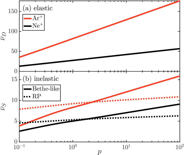
Figure 1: (a) The deflection frequency and (b) the slowing-down frequency as a function of the incoming-electron momentum, for both ${\rm Ar}^{+},$ (black) and ${\rm Ne}^{+},$ (red). These are normalized such that $\nu_{\rm D}=\tau_{\rm c}^{-1}(\gamma/p^{3})\bar{\nu}_{\rm D}$ and $\nu_{\rm s}=\tau_{\rm c}^{-1}(\gamma^{2}/p^{3})\bar{\nu}_{\rm s}$. The solid lines denote $\nu_{\rm D}$ from (5) and $\nu_{\rm s}$ from (9), respectively. The approximate Rosenbluth-Putvinski (RP) model of $\nu_{\rm s}$ [22] is shown in dotted line. Parameters: $T=10\,\mathrm{eV}$ and $n_{Z}=n_{\rm e}=10^{20}\,\mathrm{m^{-3}}$.

slowing-down frequency, we obtain, in units of $\tau_{\rm c}^{-1}$,

$$\nu_{\rm s} =\frac{\gamma^{2}}{p^{3}}\bar{\nu}_{\rm s}\,,$$

$$\bar{\nu}_{\rm s} =\frac{1}{\ln\Lambda_{\rm c}}\bigg{(}\!\ln\Lambda^{\rm ee}\!+\!\sum_{j}\!\frac{n_{j}}{n_{\rm e}}N_{{\rm e},j}\left(\ln h_{j}-\beta^{2}\right)\!\!\bigg{)}.$$ (9)

Here, $h_{j}=p\sqrt{\gamma-1}/I_{j}$ and $I_{j}$ is the mean excitation energy of the ion, normalized to the electron rest energy [12]; see table 1 in A. As $\nu_{\rm s}$ given in (9) is based on the Bethe stopping-power formula matched to the low-energy asymptote corresponding to complete screening, we refer to it as the Bethe-like model. As shown in figure 1b, the slowing-down frequency is enhanced significantly compared to the completely screened limit with constant Coulomb logarithm, where $\bar{\nu}_{\rm s}=1$. The enhancement is also significantly different from a widely used rule of thumb that is mentioned in passing by Rosenbluth and Putvinski [22], which suggests that inelastic collisions with bound electrons can be taken into account by adding half the number of bound electrons to the number of free electrons. As shown in figure 1, the Rosenbluth-Putvinski (RP) model overestimates the slowing-down frequency at low energies and is a significant underestimation at high runaway energies. The weak energy-dependence of the RP model is due to the energy-dependence in the electron-electron Coulomb logarithm in (3).

In the ultra-relativistic limit $p\gg 1$, the slowing-down frequency  (9) is approximately

$$\bar{\nu}_{\rm s}\approx(\bar{\nu}_{\rm s0}+\bar{\nu}_{\rm s1}\ln p),$$ (10)

where

$$\bar{\nu}_{\rm s0} =1+\frac{1}{\ln\Lambda_{\rm c}}\!\sum_{j}\!\frac{n_{j}}{n_{\rm e}}N_{{\rm e},j}\left(\ln I_{j}^{\scalebox{0.5}[0.7]{$-$}\!1}\!-\!1\right),$$ (11)

$$\bar{\nu}_{\rm s1} =\frac{1}{2}\frac{1}{\ln\Lambda_{\rm c}}\bigg{(}1+\!\sum_{j}3\,\frac{n_{j}}{n_{\rm e}}N_{{\rm e},j}\bigg{)}.$$ (12)

2.2 Radiation losses

At the high densities typical of post-disruption scenarios, bremsstrahlung may be an important energy loss mechanism compared to synchrotron radiation reaction [25, 26]. In a fully ionized plasma, the required density for bremsstrahlung dominance is [27]

$$n_{\rm e,20}\gtrsim B_{\rm T}^{2}\,,$$ (13)

with $B_{\rm T}$ in units of Tesla and $n_{\rm e,20}$ normalized to $10^{20}\,\mathrm{m^{-3}}$. In a partially ionized plasma, both bremsstrahlung and synchrotron losses will be enhanced, the latter through the increased pitch-angle scattering. Both radiative energy loss channels can therefore be significant at densities characteristic of disruptions and are included in this paper.

The synchrotron radiation reaction force is given by [28, 29]

$$\frac{\partial}{\partial\bi{p}}\!\cdot\!\left(\bi{F}_{\rm syn}f\right)=-\!\frac{1}{p^{2}}\frac{\partial}{\partial p}\!\left(\frac{p^{3}\gamma}{\tau_{\rm syn}}(1\!-\!\xi^{2}){f}\right)$$

$$+\frac{\partial}{\partial\xi}\left(\frac{\xi(1\!-\!\xi^{2})}{\tau_{\rm syn}\gamma}{f}\right),$$ (14)

where $\tau_{\rm syn}$ is the synchrotron radiation-damping timescale normalized to $\tau_{\rm c}$:

$$\tau_{\rm syn}^{-1}=\frac{\tau_{\rm c}e^{4}B^{2}}{6\pi\epsilon_{0}m_{\rm e}^{3}c^{3}}\approx\frac{1}{15.44\ln\Lambda_{\rm c}}\frac{B_{\rm T}^{2}}{n_{\rm e,20}}.$$ (15)

We model partially screened bremsstrahlung with a Boltzmann operator as presented in [26], using the model that neglects the angular deflection due to the bremsstrahlung process:

$$C_{\rm br}(p,\xi)=\int\!v_{1}f(p_{1},\xi)\frac{\partial{\sigma}^{\rm br}(p,p_{1})}{\partial p}\mathrm{d}p_{1}$$

$$-vf(p,\xi)\sigma^{\rm br}(p),$$

where $\partial\sigma^{\rm br}(p,p_{1})/\partial p$ is the normalized cross-section for an incident electron with momentum $p_{1}$ to end up with momentum $p$ after emitting a bremsstrahlung photon carrying the energy difference, and $\sigma^{\rm br}$ is the total bremsstrahlung cross section for an incident electron of momentum $p$. The integration is taken over $\sqrt{(\gamma+k_{\mathrm{c}})^{2}-1}\leq p_{1}<\infty$, where, following [26], photon energies are cut off at $0.1\%$ of the kinetic energy of the outgoing electrons in order to resolve the infrared divergence, i.e. $k_{c}=(\gamma-1)/1000$. The partially screened bremsstrahlung cross section is given in [30, 31]:

$$\frac{\partial{\sigma}^{\rm br}}{\partial p}(p,p_{1})=\frac{\alpha}{\pi\ln\Lambda_{\rm c}}\frac{1}{k}\sum_{j}\frac{n_{j}}{n_{\rm e}}\left[\left(1+\frac{\gamma^{2}}{\gamma_{1}^{2}}\right)\right.$$

$$\times\left(Z_{j}^{2}+\int_{q_{0}}^{1}[Z_{j}\!-\!F_{j}(q)]^{2}\frac{(q-q_{0})^{2}}{q^{3}}\mathrm{d}q\right)$$

$$-\frac{2}{3}\frac{\gamma}{\gamma_{1}}\left(\frac{5}{6}Z_{j}^{2}+\int_{q_{0}}^{1}[Z_{j}\!-\!F_{j}(q)]^{2}\right.$$

$$\left.\left.\times\frac{q^{3}+3qq_{0}^{2}[1-2qq_{0}^{2}\ln(q/q_{0})]-4q_{0}^{3}}{q^{4}}\mathrm{d}q\right)\right]$$ (16)

where $k$ is the photon momentum and $q_{0}=p_{1}-p-k$. We use the form factor $F(q)$ for partially ionized atoms presented in [9],

$$F_{j}(q)=\frac{N_{{\rm e},j}}{1+(q\bar{a}_{j})^{3/2}}\,.$$

In order to get an analytically tractable problem when deriving the effective critical electric field, a simplified bremsstrahlung mean-force stopping power will be used in section 3. Although a mean-force model has been shown to significantly alter the steady-state electron distribution compared to the full Boltzmann model, it captures the mean energy accurately [26], and is therefore sufficient for the purpose of deriving the effective critical electric field. This assumption is verified with numerical calculations using the full Boltzmann operator in section 4.

For the mean force model, we have

$$C_{\rm br}\{f\}\approx-\frac{\partial}{\partial\bi{p}}\!\cdot\!\left(\bi{F}_{\rm br}f\right)=\!\frac{1}{p^{2}}\frac{\partial}{\partial p}\!\left(p^{2}F_{\rm br}f\right),$$ (17)

where the bremsstrahlung mean force is given by $F_{\rm br}(p)=\int\,k(\partial\sigma^{\rm br}(p_{1},p)/\partial p_{1})\,\mathrm{d}p_{1}$, the integral taken over all allowed outgoing momenta $p_{1}$. For argon and neon, a numerical investigation of (16) shows that $F_{\rm br}$ is well approximated by

$$F_{\rm br} \approx p(\phi_{\rm br0}+\phi_{\rm br1}\ln p)$$ (18)

$$\equiv\frac{p\alpha}{\ln\Lambda_{\rm c}}\sum_{j}\frac{n_{j}}{n_{\rm e}}Z_{j}^{2}(0.35+0.20\ln p).$$

3 Effective critical electric field

The critical electric field is a central parameter for both generation of a runaway current and for its decay rate in a highly inductive tokamak; in the latter case, it is predicted that once the Ohmic current has dissipated, the induced electric field will be close to the critical electric field so that the current decays according to ${\rm d}I/{\rm d}t\!=\!2\pi RE_{c}^{\rm eff}/L$ [21], where $L\!\sim\!\mu_{0}R$ is the self-inductance and $R$ is the major radius of the tokamak. The physical argument is that the runaway avalanche timescale is much faster than the inductive timescale, and therefore the electric field must be close to the critical electric field to prevent rapid current variations.

We calculate the effective electrical field due to collisions with partially screened ions by finding the minimum electric field $E_{\rm c}^{\rm eff}$ that satisfies the pitch-angle averaged force-balance equation

$$\langle eE\xi-F\rangle=0\,,$$

where $F$ denotes the collisional and radiation forces on a runaway electron.

In order to find $E_{\rm c}^{\rm eff}$, we assume rapid pitch-angle dynamics compared to the timescale of the energy dynamics [32, 20]. In the kinetic equation (1), this amounts to requiring that the pitch-angle flux vanishes. Since $\tau_{\rm syn}^{-1}\ll 1$ from (15), we can neglect the effect of radiation on the pitch-angle distribution (term marked as “neglect” below) as well as the effect of the avalanche source, which is slower than both pitch-angle scattering and collisional friction. We demonstrate the validity of these assumptions in B by comparing the resulting critical electric field and angular distribution to kinetic simulations. Inserting the collision frequencies (6) and (10) as well as the radiation terms (14) and (17), the kinetic equation (1) can be rewritten

$$\frac{\partial\bar{f}}{\partial\tau}=\frac{\partial}{\partial p}\left[\left(-\frac{\xi E}{E_{\rm c}}+p\nu_{\rm s}+F_{\rm br}+\frac{p\gamma}{\tau_{\rm syn}}(1\!-\!\xi^{2})\right)\bar{f}\right]$$

$$+\frac{\partial}{\partial\xi}\bigg{[}(1-\xi^{2})\underbrace{\left(-\frac{1}{p}\frac{E}{E_{\rm c}}\bar{f}+\frac{1}{2}\nu_{\rm D}\frac{\partial\bar{f}}{\partial\xi}\right)}_{=0}-\underbrace{\frac{\xi(1\!-\!\xi^{2})}{\tau_{\rm syn}\gamma}}_{\rm neglect}\bar{f}\bigg{]}\,$$ (19)

where $\bar{f}=p^{2}f$.

Following the method and notation of [20], the condition that the pitch-angle flux vanishes yields the following form for the angular distribution:

$$\bar{f}=G(t,p)A\exp(A\xi)/2\sinh A,$$ (20)

where the parameter $A$ is defined as

$$A(p)\equiv\frac{2E}{p\nu_{\rm D}E_{\rm c}}.$$

Then, (19) integrated over pitch-angle yields a continuity equation

$$\frac{\partial G}{\partial\tau}+\frac{\partial}{\partial p}\left[U(p)G\right]=0,$$

where

$$U(p)=\frac{E/E_{\rm c}}{\tanh A}-\left[p\nu_{\rm s}+F_{\rm br}+\frac{p\nu_{\rm D}}{2}\right.$$

$$+\left.\frac{p^{2}\gamma\nu_{\rm D}}{\tau_{\rm syn}E/E_{\rm c}}\left(\frac{1}{\tanh A}-\frac{1}{A}\right)\right].$$ (21)

As the sign of $U(p)$ determines if the distribution at $p$ is accelerated or decelerated, the effective critical electric field is the minimum electric field for which force balance is possible:

$$E_{\rm c}^{\rm eff} \equiv\min_{p}\left[E\big{|}U(p,E)=0\right].$$ (22)

The minimum can be found analytically if $A\!\gg\!1$ (so that $\tanh A\approx 1$) and the critical momentum fulfills $p_{\rm c}(E_{\rm c}^{\rm eff})\!\gg\!1$, which are consistent with our final solution if partially ionized impurities dominate. Hence (6), (10) and (18) may be used, and (22) is approximately solved by (see C for more details): 

$$\frac{E_{\rm c}^{\rm eff}}{E_{\rm c}}\approx \ \bar{\nu}_{\rm s0}+\bar{\nu}_{\rm s1}\!\left[\!\left(1\!+\!\frac{\bar{\nu}_{\rm D1}}{\bar{\nu}_{\rm D0}}\right)\ln\!\frac{\bar{\nu}_{\rm D0}}{2\bar{\nu}_{\rm s1}}+\sqrt{2\delta+1}\right],$$ (23)

where the constants are given in (2), (7), (8), (11), (12), (15), and (18), and $\delta$, which is a measure of the effect of radiation losses, is given by

$$\delta(E_{\rm c}^{\rm eff})=\frac{\bar{\nu}_{\rm D0}}{\bar{\nu}_{\rm s1}^{2}}\left(\frac{\bar{\nu}_{\rm D0}\tau_{\rm syn}^{-1}}{E_{\rm c}^{\rm eff}/E_{\rm c}}+\phi_{\rm br0}+\phi_{\rm br1}\ln(\bar{\nu}_{\rm D0}/2\bar{\nu}_{\rm s1})\right).$$ (24)

Since $\delta$ depends on $E_{\rm c}^{\rm eff}$, (23) is not in a closed form, and therefore (23) and (24) are evaluated iteratively starting at $E_{\rm c}^{\rm eff}=E_{\rm c}^{\rm tot}$, where $E_{\rm c}^{\rm tot}$ is the critical electric field including the density of both bound and free electrons:

$$E_{\rm c}^{\rm tot}\equiv\frac{n_{\rm e}^{\rm tot}}{n_{\rm e}}E_{\rm c}=\frac{n_{\rm e}^{\rm tot}e^{3}\ln\Lambda_{\rm c}}{4\pi\epsilon_{0}^{2}m_{\rm e}c^{2}},$$ (25)

with $n_{\rm e}^{\rm tot}=n_{\rm e}+\sum_{j}n_{j}N_{{\rm e},j}$. Here, we iterate once so that $\delta_{0}=\delta(E_{\rm c}^{\rm eff}\!=\!E_{\rm c}^{\rm tot})$ and $\delta\approx\delta_{1}=\delta[E_{\rm c}^{\rm eff}(\delta_{0})]$. Equation (23) was found to be accurate to within 10% for magnetic fields in the range $B_{\rm T}^{2}\!\lesssim\!100\,n^{\rm tot}_{20}$ for all considered impurity species and plasma compositions.

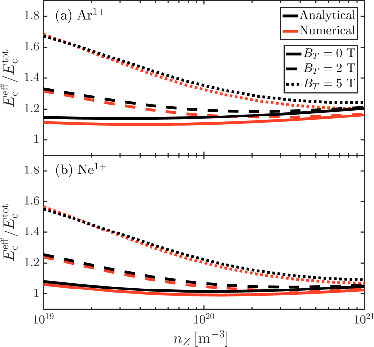
Figure 2: Effective critical electric field normalized to $E_{\rm c}^{\rm tot}$ (25) as function of $n_{Z}$, where $n_{Z}$ is the density of Ar⁺ (top) and Ne⁺ (bottom). The analytical expression (23) is plotted in black, and the numerical solutions to (22) are illustrated in red. The magnetic field is $B=0\,\mathrm{T}$ (solid line), $B=2\,\mathrm{T}$ (dashed line) and $B=5\,\mathrm{T}$ (dotted line). Parameters: $T=10\,\mathrm{eV}$, $n_{\rm D}=10^{20}\,\mathrm{m^{-3}}$.

Figure 2 shows the effective critical electric field normalized to $E_{\rm c}^{\rm tot}$. Our model, corresponding to (23), is shown in black and compared to the full numerical solution to (22) (using the algorithm in [33], implemented as fmincon in matlab) for three different values of the magnetic field: $B=0\,\mathrm{T}$ in solid line, $B=2\,\mathrm{T}$ dashed and $B=5\,\mathrm{T}$ in dotted line. These are shown for singly ionized argon in figure 2(a) and singly ionized neon in 2(b). The behavior is only weakly dependent on ionization states; this is illustrated with neutral argon and Ar⁴⁺ in figure 3. In addition, we find that the background deuterium density has a negligible effect on $E_{\rm c}^{\rm eff}$ when $Zn_{Z}\gg n_{\rm D}$.

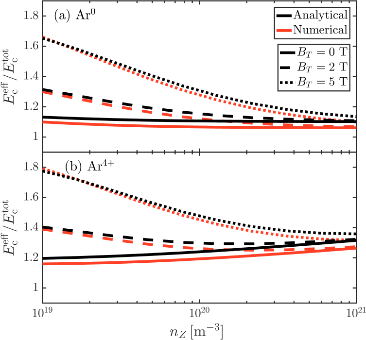
Figure 3: Effective critical electric field normalized to $E_{\rm c}^{\rm tot}$ (25) as function of $n_{Z}$, where $n_{Z}$ is the density of (a) Ar⁰ and (b) Ar⁴⁺. The black lines correspond to the analytical expression (23), and the red lines are the numerical solutions to (22). The magnetic field is $B=0\,\mathrm{T}$ (solid line), $B=2\,\mathrm{T}$ (dashed line) and $B=5\,\mathrm{T}$ (dotted line). Parameters: $T=10\,\mathrm{eV}$, $n_{\rm D}=10^{20}\,\mathrm{m^{-3}}$.

Figures 2-3 also show that with weakly ionized impurities,

$$E_{\rm c}^{\rm eff}\gtrsim E_{\rm c}^{\rm tot}\gg E_{\rm c}.$$

Hence, it is more accurate to include all electrons in the critical electric field, than to count for instance half of the bound electrons as done in the Rosenbluth-Putvinski model ($E_{\rm c}^{\rm RP}=E_{\rm c}^{\rm tot}(n_{\rm e}+0.5n_{\rm bound})/n_{\rm e}^{\rm tot}$). This underestimation of the effective critical field by the RP model is a result of using a simplistic form of the inelastic collision rate as well as neglecting the effect of pitch-angle scattering and radiation losses. To further explore the scaling of $E_{\rm c}^{\rm eff}$ with magnetic field strength and impurity content, we approximate (23) in the case where one weakly ionized state $j$ dominates:

$$\frac{E_{\rm c}^{\rm eff}}{E_{\rm c}^{\rm tot}}\!\approx\frac{n_{\rm e}}{n_{\rm e}^{\rm tot}}\!+\!\frac{N_{{\rm e},j}n_{Z}}{n_{\rm e}^{\rm tot}}\frac{1}{\ln\Lambda_{\rm c}}\!\!\left(\!S_{j}\!+\!R_{j}\sqrt{\frac{B_{\rm T}^{2}}{n_{20}^{\rm tot}}\!+\!\frac{0.9}{\ln\bar{a}_{j}}}\!\right)\!,\!$$ (26)

$$S_{j}=\left[\ln I_{j}^{-1}\!-\!1\!+\!\frac{3}{2}\left(\!1\!+\!\frac{1}{\ln\bar{a}_{j}}\right)\ln\!\left(\!\frac{Z_{j}}{3}\ln\bar{a}_{j}\right)\right],\!$$ (27)

$$R_{j}=0.09(Z\!+\!Z_{0})\ln\bar{a}_{j}.$$ (28)

The screening constant $S_{j}$ is given for all argon and neon species in table 1 in A. For typical magnetic fields, the terms inside the brackets tend to be roughly 1-2 times $\ln\Lambda_{\rm c}$. As $n_{\rm e}\!+\!N_{{\rm e},j}n_{j}\!=\!n_{\rm e}^{\rm tot}$ with only one impurity species $j$, one obtains $E_{\rm c}^{\rm eff}\!\gtrsim\!E_{\rm c}^{\rm tot}$. From (26), we thus conclude that the effect of partially stripped impurities scale approximately linearly with impurity density; more specifically, $E_{\rm c}^{\rm eff}=E_{\rm c}^{\rm tot}(n_{\rm e}+\kappa n_{\rm bound})/n_{\rm e}^{\rm tot}\approx\kappa E_{\rm c}^{\rm tot}$, where $\kappa$ is between 1 and 2. Consequently, our calculated of $E_{\rm c}^{\rm eff}$ is up to $4E_{\rm c}^{\rm RP}$ in typical tokamak scenarios.

The radiation term $R_{j}$ quantifies the effect of bremsstrahlung and synchrotron losses; these are dominated by synchrotron radiation reaction if

$$B_{\rm T}^{2}\gtrsim 0.2n_{20}^{\rm tot}\,,$$

which is lower than the fully ionized estimation (13). In this case, $E_{\rm c}^{\rm eff}$ depends linearly on $B_{\rm T}/\sqrt{n_{20}^{\rm tot}}$ . This agrees with the scaling found in [20] for the fully ionized case. In contrast, for low magnetic fields, bremsstrahlung can increase the effective critical field by up to 20% for argon. This number is insensitive to the plasma density and depends only on its ionic composition.

4 Current decay

The critical electric field, especially as modified by the effects of partially screened nuclei and radiation losses, plays an important role during the relaxation of runaway electrons. In this section, we demonstrate with kinetic simulations that (23) well characterizes the threshold between runaway growth and decay under these modifications. Then, when the electric field evolves self-consistently, we show that it remains tied to $E_{\rm c}^{\rm eff}$ under certain assumptions during the current decay phase of a tokamak disruption.

If the current is carried by runaway electrons and the shape of the runaway distribution is constant in time, the time derivative of the current is related to the steady-state runaway growth rate

$$\Gamma(E)\equiv\frac{1}{n_{\rm RE}}\frac{\mathrm{d}n_{\rm RE}}{\mathrm{d}t}\approx\frac{1}{I}\frac{\mathrm{d}I}{\mathrm{d}t}.$$ (29)

The scaling of the growth rate with impurity content may be estimated from the Rosenbluth–Putvinski formula [22] by replacing $E_{\rm c}$ with $E_{\rm c}^{\rm eff}$ and the density by the total electron density due to the fact that bound and free electrons have equal probability of becoming runaway electrons through knock-on collisions:

$$\Gamma(E)\sim\frac{1}{\ln\Lambda_{\rm c}}\frac{1}{\tau_{\rm c}^{\rm tot}}\left(\frac{E}{E_{\rm c}^{\rm eff}}-1\right),$$ (30)

with $\tau_{\rm c}^{\rm tot}\!=\!(n_{\rm e}/n_{\rm e}^{\rm tot})\tau_{\rm c}$. The qualitative scaling of the analytic growth rate is confirmed in figure 4, where the growth rate is numerically calculated using code [34, 35], which directly solves the kinetic equation (1). These simulations employed the general field-particle knock-on operator of [36, 37, 38] and a Boltzmann operator for partially screened bremsstrahlung losses as described in section 2.2. The vertical lines denote the analytic prediction in (23) for when one would expect the transition between growth and decay of an existing runaway population. Radiation losses affect where this threshold lies and the analytic model $E_{\rm c}^{\rm eff}$ accurately and robustly captures this effect. In particular, we note that the mean-force bremsstrahlung model employed in the analytical derivation of $E_{\rm c}^{\rm eff}$ agrees with the Boltzmann-type bremsstrahlung operator used in the simulations within a few percent.

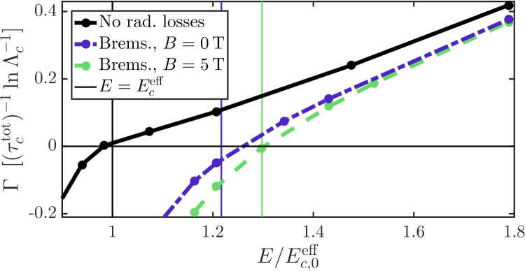
Figure 4: Steady-state runaway growth rate as a function of electric field normalized to the critical electric field $E_{c,0}^{\rm eff}$ without radiation losses. The solid black line is without radiation losses; the dash-dotted blue line includes bremsstrahlung and the dashed green line includes both bremsstrahlung and synchrotron losses corresponding to $B=5\,\mathrm{T}$. The vertical lines denote the analytical prediction $E=E_{\rm c}^{\rm eff}$. Parameters: $n_{\rm D}=10^{20}\,\mathrm{m^{-3}}$, a density of Ar⁺ given by $n_{\rm Ar}=4n_{\rm D}$ and $T=10\,\mathrm{eV}$.

The electric field is hypothesized to remain close to $E_{\rm c}^{\rm eff}$ during the current-decay phase of a tokamak disruption [21]. The mechanism by which this occurs is the fast timescale of the avalanche generation in relation to the inductive timescale of the system. A toroidal electric field is induced when there is a time-changing magnetic flux through a current loop such as a runaway beam. This magnetic flux is proportional to the total current through the loop. The induced electric field is therefore related to the rate of change of the current:

$$E=-\frac{L}{2\pi R}\frac{{\rm d}I}{{\rm d}t},$$ (31)

where $R$ is the major radius of the tokamak. This inductance model has recently been implemented in code to calculate the electric field self-consistently with the evolution of the electron velocity distribution. In general, the exact value of the inductance $L$ will depend on the spatial distribution of current, which will change in time. For a large-aspect ratio current loop (such as a runaway beam), $L$ can be approximated by [39]

$$L\approx\mu_{0}R\left[\ln\left(\frac{8R}{a}\right)-2+\frac{l_{i}}{2}\right].$$ (32)

Here, $R$ is the major radius of the tokamak, $a$ is the radius of the runaway beam, and $l_{i}$ parametrizes the distribution of current within the beam. We have chosen $l_{i}=1.5$ as a representative mid-plateau value, based on experimental results from European medium sized tokamaks.

When $E\approx E_{\rm c}^{\rm eff}$, the growth rate can be expanded according to

$$\Gamma=\Gamma^{\prime}\!(\!E_{\rm c}^{\rm eff}\!)[E-E_{\rm c}^{\rm eff}]+\dots,$$

which allows (31) to be solved analytically:

$$E\approx E_{\rm c}^{\rm eff}\left(1-\frac{2\pi R}{LI_{\rm RE}\Gamma^{\prime}\!(\!E_{\rm c}^{\rm eff}\!)}\right).$$ (33)

This yields a condition under which the electric field remains close to $E_{\rm c}^{\rm eff}$:

$$LI_{\rm RE}\Gamma^{\prime}\!(\!E_{\rm c}^{\rm eff}\!)\gg 2\pi R.$$

With the estimate of $\Gamma^{\prime}\!(\!E\!)$ from the numerical results of figure 4 (at $B=0\,\mathrm{T}$) and estimating $R/a\!\approx\!5$ we find that the minimum required current for $E\!\approx\!E_{\rm c}^{\rm eff}$ is approximately

$$I_{\rm RE}\,\gg 60\,\mathrm{kA}.$$ (34)

This value is substantially lower than the estimation of 250 kA in [21], which did not include the effect of partial screening or radiation losses. Since this threshold current is inversely proportional to the inductance, the estimate (34) is only weakly dependent on the details of the spatial current distribution. Therefore, the exact value of the instantaneous inductance does not affect the primary result of this section: for large enough inductance, the electric field remains approximately tied to $E_{\rm c}^{\rm eff}$ during the current decay phase, leading to a predictable decay time scale.

To test the hypothesis that $E\!\approx\!E_{\rm c}^{\rm eff}$ when $I_{\rm RE}\!\gg\!60\,\mathrm{kA}$, we generate a forward-beamed initial distribution obtained from a simulation with a large electric field; the initial average runaway energy in our simulation is 17.2 MeV. We then inject singly ionized argon with a density that is four times the deuterium density $n_{\mathrm{D}}\!=\!10^{20}\,\mathrm{m^{-3}}$. Starting at an initial current density $j_{0}\!=\!12.9\,\mathrm{MA/m^{2}}$, we let the electron distribution evolve with a self-consistent electric field in a strongly, intermediate or weakly inductive system. At a constant current density, varying $I_{0}^{\rm RE}L/(\mu_{0}R)$ corresponds to varying $L/(\mu_{0}R)$ through the beam aspect ratio $R/a$ or the initial current $I_{0}\!=\!j_{0}\pi a^{2}$. The following values were chosen in the simulations: $\pi a^{2}L/(\mu_{0}R)\!=\!(i)\,4.30\,,(ii)\,1.57\,{\rm and}\,(iii)\,0.14$. If $R/a\!=\!5$ and $l_{i}=1.5$, these three values correspond to an initial current of $(i)\,I_{0}^{\rm RE}\!=\!23\,\mathrm{MA}$; $(ii)\,I_{0}^{\rm RE}\!=\!8.3\,\mathrm{MA}$; and $(iii)\,I_{0}^{\rm RE}\!=\!0.75\,\mathrm{MA}$. As in the growth rate simulations, we include both synchrotron losses, the full bremsstrahlung model and a Chiu-Harvey type avalanche operator.

Figure 5a shows the current decay, which is linear (as expected) and faster in the low inductance case. Figure 5b shows the electric field evolution. Clearly, in the high-inductance case, the electric field is close to the critical field after an initial transient. This means that, in highly inductive devices such as ITER, the current decay is to a very good approximation given by ${\rm d}I_{\rm RE}/{\rm d}t=-2\pi RE_{\rm c}^{\rm eff}/L$. Enhanced $E_{\rm c}^{\rm eff}$ will lead to faster current decay, and (23) quantifies how fast the decay is.

On the other hand, the induced electric field deviates by approximately 10% from $E_{\rm c}^{\rm eff}$ in the low-inductance case. Since the initial current $I_{0}^{\rm RE}\!=\!750\,\mathrm{kA}$ is high in relation to many medium-sized tokamak experiments, $E\!\approx\!E_{\rm c}^{\rm eff}$ gives an overestimation of the current decay rate in many of today’s devices. The relative deviation from $E_{\rm c}^{\rm eff}$ observed in figure 5b is consistent with the estimation $1-E/E_{\rm c}^{\rm eff}\approx 60\,\mathrm{kA}/I_{\rm RE}$ from (33) and (34).

Although the predicted induced electric field obeys $E\!\leq\!E_{\rm c}^{\rm eff}$ with our assumptions, several effects could lead to a higher induced electric field in an actual experimental discharge. For example, a stronger electric field would be necessary to balance a runaway population with sub-relativistic energy, in which case the steady-state growth rate used here is inaccurate. Other effects such as transport [40, 41, 42], trapping [22, 43] and wave-particle interaction [10, 44, 45, 46] may also increase the runaway current decay rate and accordingly the induced electric field. Such complete modelling remains the subject of future work. Nevertheless, partial screening has a major effect on the critical electric field as demonstrated here, and therefore the results derived herein should be an important piece toward improved experimental comparison of the runaway current decay rate as well as the avalanche growth rate.

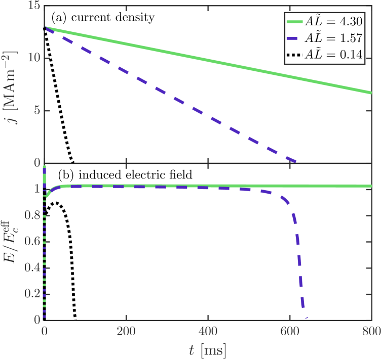
Figure 5: Current decay (top) and electric field (bottom) for $T=10\;\rm eV$, Ar⁺ with $n_{\mathrm{Ar}}\!=\!4n_{\mathrm{D}}$, $n_{\mathrm{D}}\!=\!10^{20}$ m^-3, for three different inductance parameters $A\tilde{L}\equiv\pi a^{2}L/(\mu_{0}R)$ in solid blue, dashed green and dotted black line respectively. The initial average runaway energy was 17.2 MeV. Bremsstrahlung losses were included here, and $B=0\,\mathrm{T}$ for simplicity.

Finally, we note that the simulations with an inductive electric field validate the initial assumption of rapid pitch-angle dynamics in (19); we find that the resulting pitch-angle distribution in (20) is accurate for $E\!\approx\!E_{\rm c}^{\rm eff}$; see B. The distribution function in (20) is consequently appropriate for determining the effective critical electric field, but not for describing runaway generation.

5 Conclusion

Recent experimental studies on several tokamaks show that the onset and decay of runaway electrons occurs for critical electric fields that are considerably higher than the Connor–Hastie field $E_{\rm c}$. One reason is that there are other runaway loss mechanisms in addition to damping due to collisions in a fully ionized plasma that seem to dominate both in disruptive and quiescent cases. In this paper, we show that if there are heavy partially ionized impurities present in the plasma, the dominant effect on the critical electric field is the effect of partial screening. The effective critical field is further increased due to the enhanced radiation loss rates when partially ionized impurities are present.

We give analytical formulas for the effective critical electric field $E_{\rm c}^{\rm eff}$ including partial screening and radiation effects, derived under the condition of rapid pitch-angle dynamics. The validity of this assumption and the value of the effective critical electric field is demonstrated by numerical simulations with the kinetic equation solver code. The most complete expression for the critical electric field is given in (23). It has been shown to be valid for a wide range of magnetic fields, impurity species and plasma composition. To make the parametric dependencies more transparent, we also give an approximate expression in (26) that is valid when one weakly ionized state dominates, which is often the case in a cold post-disruption tokamak plasma.

As expected, we find that in the presence of large amounts of heavy impurities, the effective critical field can be drastically higher than $E_{\rm c}$ which is proportional to the density of free electrons: $E_{\rm c}^{\rm eff}$ even exceeds the value obtained by including the total density of both free and bound electrons. In contrast to Rosenbluth–Putvinski [22], where the effective density includes half of the bound electrons, $n=n_{\rm e}+0.5n_{\rm bound}$, our calculations show that the bound electrons are weighted by a factor of typically 1-2. This enhancement is attributed to the energy-dependent collisional friction, pitch-angle scattering as well as radiation losses. Bremsstahlung and synchrotron losses both increase the effective critical field, typically by tens of percent.

Using a 0D inductive electric field we calculate the runaway current decay after impurity injection. Through kinetic simulations we confirm the accuracy of the formula for the effective critical field (23), and demonstrate that the electric field stays close to the effective critical field when the runaway current satisfies $I_{\rm RE}\!\gg\!60\,\mathrm{kA}$, in which case ${\rm d}I_{\rm RE}/{\rm d}t\propto E_{\rm c}^{\rm eff}$. These findings are relevant for the efficacy of mitigation strategies for runaway electrons in tokamak devices: since the runaway current decay rate is typically 2-4 times higher than what is predicted by the Rosenbluth–Putvinski formula, a lower quantity of assimilated material is required for successful mitigation. As screening significantly increases the critical electric field, we anticipate that this effect is of importance to include in experimental comparisons; however, accurate predictions may require the modelling of spatial effects which are not considered here.

Appendix A Constants for the effective electric field

Table 1 summarizes the constants needed to compute the value of the effective electric field in the presence of argon and neon. The effective ion size $\bar{a}_{j}$ is determined by DFT simulations and is related to $a_{j}$ in [9] through $\bar{a}_{j}=2a_{j}/\alpha$ where $\alpha\approx 1/137$ is the fine-structure constant. The mean excitation energy $I_{j}$ is taken from [12]. These give $S_{j}$ from (27) according to

$$S_{j}=\left[\ln I_{j}^{-1}\!-\!1\!+\!\frac{3}{2}\left(\!1\!+\!\frac{1}{\ln\bar{a}_{j}}\right)\ln\!\left(\!\frac{Z_{j}}{3}\ln\bar{a}_{j}\right)\right].$$

Table 1: Constants to determine $E_{\rm c}^{\rm eff}$.

• 	$\ln\bar{a}_{j}$	$\ln I_{j}^{\scalebox{0.5}[0.7]{$-$}\!1}$	$S_{j}$			$\ln\bar{a}_{j}\!$	$\ln I_{j}^{\scalebox{0.5}[0.7]{$-$}\!1}$	$S_{j}$
  Ar0	4.6	7.9	13.0		Ne0	4.7	8.2	12.2
  Ar1+	4.5	7.8	12.8		Ne1+	4.6	8.0	12.0
  Ar2+	4.4	7.6	12.6		Ne2+	4.5	7.9	11.8
  Ar3+	4.4	7.5	12.5		Ne3+	4.4	7.7	11.6
  Ar4+	4.3	7.3	12.3		Ne4+	4.3	7.5	11.4
  Ar5+	4.2	7.2	12.2		Ne5+	4.1	7.3	11.2
  Ar6+	4.1	7.0	12.0		Ne6+	4.0	7.0	10.8
  Ar7+	4.0	6.8	11.8		Ne7+	3.7	6.6	10.4
  Ar8+	3.9	6.6	11.5		Ne8+	3.2	5.9	09.5
  Ar9+	3.8	6.5	11.4		Ne9+	3.1	5.8	09.5
  Ar10+	3.7	6.4	11.3
  Ar11+	3.6	6.2	11.1
  Ar12+	3.6	6.1	11.0
  Ar13+	3.5	5.9	10.8
  Ar14+	3.3	5.7	10.5
  Ar15+	3.1	5.3	10.1
  Ar16+	2.6	4.7	09.4
  Ar17+	2.5	4.7	09.4

Appendix B Angular dependence of the runaway electron distribution function

The simulations with an inductive electric field (figure 5) can be used to validate the initial assumption of rapid pitch-angle dynamics in (19) leading to the pitch-angle distribution in (20). Expanding $\bar{f}$ in Legendre polynomials

$$\bar{f}=\sum_{L}\bar{f}_{L}(p)P_{L}(\xi),$$

we relate the predicted analytical distribution in (20) to the ratio between the zeroth and the first Legendre modes of the distribution:

$$\frac{1}{3}\frac{\bar{f}_{1}}{\bar{f}_{0}}=\left(\frac{1}{\tanh A}-\frac{1}{A}\right).$$ (35)

The ratio given in (35) quantifies the narrowness of the electron distribution: $\bar{f}_{1}/3\bar{f}_{0}=0$ corresponds to an isotropic distribution while the $\bar{f}_{1}/3\bar{f}_{0}\rightarrow 1$ for a narrow, beam-like distribution. Figure 6 compares the numerical value of $\bar{f}_{1}/3\bar{f}_{0}$ as computed in code in solid black line, to the analytical prediction (35) in dashed green line. The analytical formula accurately predicts the distribution width on the entire interval from a fully isotropic distribution at $p=0$ to a narrow beam for $p\gg 1$. This validates our assumptions on the rapid pitch-angle dynamics in (19). In contrast, for larger electric fields ($E/E_{\rm c}^{\rm eff}\gtrsim 5$), we find that the distribution rather follows the formula in Fülöp et al. [47], which is derived in the limit of $E\gg E_{\rm c}^{\rm eff}$.

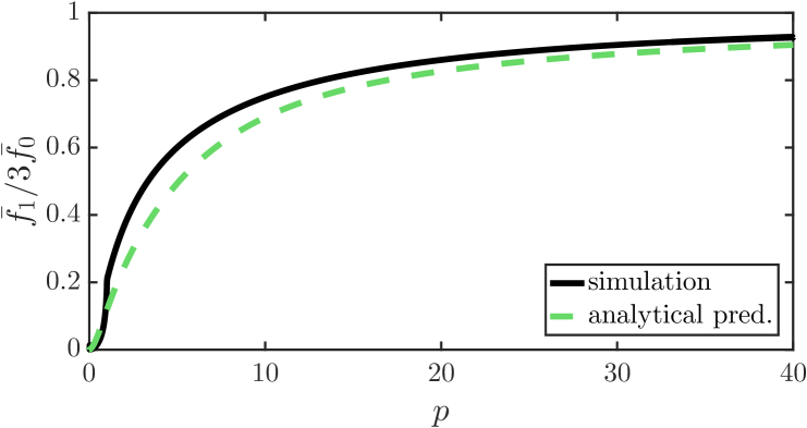
Figure 6: The distribution width parameter $\bar{f}_{1}/3\bar{f}_{0}$ as a function of momentum $p$ taken after 200 ms for the high inductance case in figure 5. This snapshot is representative for all times and for both the intermediate and the high-inductance cases.

Appendix C Derivation of the effective critical field

The effective critical field can be found analytically noting that the critical momentum fulfills $p_{\rm c}^{\star}\equiv p_{\rm c}(E_{\rm c}^{\rm eff})\!\gg\!1$. Moreover, we assume that $A$, which is defined in (20), fulfills $A\!\gg\!1$ (so that $\tanh A\approx 1$). These two assumptions are consistent with our final solution if partially ionized impurities dominate. Hence (6), (10) and (18) may be used in the expression for the effective critical field (22), and the requirement $U(p)=0$ [with $U$ given in (21)] results in a quadratic equation in $E/E_{\rm c}$:

$$\left(\frac{E}{E_{\rm c}}\right)^{2}-\frac{E}{E_{\rm c}}h(p)-\epsilon(p)=0,$$ (36)

where $h(p)$ and $\epsilon(p)$ are both positive functions of $p$ within the assumption $p_{\rm c}\!\gg\!1$:

$$h(p)\equiv\bar{\nu}_{\rm s0}+\bar{\nu}_{\rm s1}\ln p+\frac{1}{2p}(\bar{\nu}_{\rm D0}+\bar{\nu}_{\rm D1}\ln p)$$

$$+p(\phi_{\rm br0}+\phi_{\rm br1}\ln p),$$

$$\epsilon(p)\equiv p(\bar{\nu}_{\rm D0}+\bar{\nu}_{\rm D1}\ln p)\tau_{\rm syn}^{-1}.$$

Consequently, finding the effective critical field amounts to evaluating the positive solution to (36)

$$\frac{E_{\rm c}^{\rm eff}}{E_{\rm c}}\approx\frac{1}{2}\left[h(p_{\rm c}^{\star})+\sqrt{h(p_{\rm c}^{\star})^{2}+4\epsilon(p_{\rm c}^{\star})}\right]$$ (37)

at the minimum $p_{\rm c}^{\star}$, the critical momentum which minimizes $E_{\rm c}^{\rm eff}$ in (36), which is determined by

$$\frac{E_{\rm c}^{\rm eff}}{E_{\rm c}}h^{\prime}(p_{\rm c}^{\star})+\epsilon^{\prime}(p_{\rm c}^{\star})=0.$$ (38)

The derivatives of $h(p)$ and $\epsilon(p)$ are given by

$$h^{\prime}(p_{\rm c}^{\star}) \approx\frac{\bar{\nu}_{\rm s1}}{p_{\rm c}^{\star}}-\frac{1}{2(p_{\rm c}^{\star})^{2}}\left[\bar{\nu}_{\rm D0}+\bar{\nu}_{\rm D1}(\ln p_{\rm c}^{\star}-1)\right]+\phi_{\rm br0}+\phi_{\rm br1}(\ln p_{\rm c}^{\star}+1),$$

$$\epsilon^{\prime}(p_{\rm c}^{\star}) \approx\tau_{\rm syn}^{-1}[\bar{\nu}_{\rm D0}+\bar{\nu}_{\rm D1}(\ln p_{\rm c}^{\star}+1)],$$

and thus (38) is solved by

$$p_{\rm c}^{\star}\approx\frac{2p_{\rm c0}^{\star}}{1+\sqrt{1+2\delta}}\,,$$

where

$$\delta\equiv\frac{\bar{\nu}_{\rm D0}+\bar{\nu}_{\rm D1}(\ln p_{\rm c}^{\star}\!-\!1)}{\bar{\nu}_{\rm s1}^{2}}[\phi_{\rm br0}+\phi_{\rm br1}(\ln p_{\rm c}^{\star}+1)](x_{\rm rad}+1),$$ (39)

$$p_{\rm c0}^{\star}\equiv\frac{\bar{\nu}_{\rm D0}+\bar{\nu}_{\rm D1}(\ln p_{\rm c}^{\star}\!-\!1)}{2\bar{\nu}_{\rm s1}},$$ (40)

$$x_{\rm rad}\equiv\frac{[\bar{\nu}_{\rm D0}+\bar{\nu}_{\rm D1}(\ln p_{\rm c}^{\star}+1)]\tau_{\rm syn}^{-1}}{[\phi_{\rm br0}+\phi_{\rm br1}(\ln p_{\rm c}^{\star}+1)]E_{\rm c}^{\rm eff}/E_{\rm c}}.$$ (41)

Here, $x_{\rm rad}$ describes the relative importance of synchrotron radiation compared to bremsstrahlung.

To evaluate (37), we first simplify $h(p_{\rm c}^{\star})$ using $(1+\sqrt{1+2\delta})^{-1}=(\sqrt{1+2\delta}-1)/2\delta$:

$$h(p_{\rm c}^{\star})=\bar{\nu}_{\rm s0}+\bar{\nu}_{\rm s1}\ln p_{\rm c}^{\star}+\frac{\bar{\nu}_{\rm s1}}{2}\frac{(\bar{\nu}_{\rm D0}+\bar{\nu}_{\rm D1}\ln p_{\rm c}^{\star})}{\bar{\nu}_{\rm D0}+\bar{\nu}_{\rm D1}(\ln p_{\rm c}^{\star}-1)}\big{(}1+\sqrt{2\delta+1}\big{)}$$

$$+\frac{\bar{\nu}_{\rm s1}}{2}\frac{\phi_{\rm br0}+\phi_{\rm br1}\ln p_{\rm c}^{\star}}{\phi_{\rm br0}+\phi_{\rm br1}(\ln p_{\rm c}^{\star}+1)}\frac{\sqrt{1+2\delta}-1}{x_{\rm rad}+1}$$

$$\qquad\approx\underbrace{\bar{\nu}_{\rm s0}+\bar{\nu}_{\rm s1}\left(\ln p_{\rm c}^{\star}+1+\frac{\bar{\nu}_{\rm D1}}{\bar{\nu}_{\rm D0}}\ln p_{\rm c}^{\star}\right)}_{\equiv h_{0}(p_{\rm c}^{\star})}$$

$$+\frac{\bar{\nu}_{\rm s1}}{2}\big{(}\sqrt{1+2\delta}-1\big{)}\left(\frac{x_{\rm rad}+2}{x_{\rm rad}+1}\right),$$ (42)

where we assumed $\bar{\nu}_{\rm D0}\gg\bar{\nu}_{\rm D1}(\ln p_{\rm c}^{\star}-1)$ since $\bar{\nu}_{\rm D0}\gg\bar{\nu}_{\rm D1}$ typically; see (7) and (8). Furthermore, we assumed $\phi_{\rm br1}\ll\phi_{\rm br0}+\phi_{\rm br1}\ln p_{\rm c}^{\star}$. To simplify $\epsilon(p_{\rm c}^{\star})$, we approximate $E_{\rm c}^{\rm eff}/E_{\rm c}\approx h(p_{\rm c}^{\star})$ and assume $\bar{\nu}_{\rm D1}\ll\bar{\nu}_{\rm D0}+\bar{\nu}_{\rm D1}\ln p_{\rm c}^{\star}$:

$$\epsilon(p_{\rm c}^{\star}) =\frac{\bar{\nu}_{\rm s1}}{2}E_{\rm c}^{\rm eff}\big{(}\sqrt{1+2\delta}-1\big{)}\frac{\bar{\nu}_{\rm D0}+\bar{\nu}_{\rm D1}\ln p_{\rm c}^{\star}}{\bar{\nu}_{\rm D0}+\bar{\nu}_{\rm D1}(\ln p_{\rm c}^{\star}+1)}\left(\frac{x_{\rm rad}}{x_{\rm rad}+1}\right)$$ (43)

$$\approx\frac{\bar{\nu}_{\rm s1}}{2}h(p_{\rm c}^{\star})\big{(}\sqrt{1+2\delta}-1\big{)}\left(\frac{x_{\rm rad}}{x_{\rm rad}+1}\right).$$

Then,

$$\sqrt{h(p_{\rm c}^{\star})^{2}+4\epsilon(p_{\rm c}^{\star})} \approx\sqrt{h_{0}(p_{\rm c}^{\star})+\frac{\bar{\nu}_{\rm s1}}{2}\big{(}\sqrt{1+2\delta}-1\big{)}\frac{x_{\rm rad}+2}{x_{\rm rad}+1}}$$ (44)

$$\quad\times\sqrt{h_{0}(p_{\rm c}^{\star})+\frac{\bar{\nu}_{\rm s1}}{2}\big{(}\sqrt{1+2\delta}-1\big{)}\frac{5x_{\rm rad}+2}{x_{\rm rad}+1}}$$

$$\approx\left(h_{0}(p_{\rm c}^{\star})+\frac{\bar{\nu}_{\rm s1}}{2}\big{(}\sqrt{1+2\delta}-1\big{)}\frac{3x_{\rm rad}+2}{x_{\rm rad}+1}\right),$$

where the last approximation is a matching between the behavior at $x_{\rm rad}\gg 1$ and $x_{\rm rad}\ll 1$ for $2h_{0}(p_{\rm c}^{\star})\gg\bar{\nu}_{\rm s1}(\sqrt{1+2\delta}-1)$, i.e. screening effects dominate over radiation reaction effects. This assumption also motivates the approximation

$$\ln p_{\rm c}^{\star}\approx\ln p_{\rm c0}^{\star}\approx\ln(\bar{\nu}_{\rm D0}/2\bar{\nu}_{\rm s1}).$$ (45)

Finally, the effective critical field (37) is the mean of (42) and (44):

$$\frac{E_{\rm c}^{\rm eff}}{E_{\rm c}} \approx h_{0}(p_{\rm c}^{\star})+\bar{\nu}_{\rm s1}\left(\sqrt{1+2\delta}-1\right)$$ (46)

$$\approx \bar{\nu}_{\rm s0}+\bar{\nu}_{\rm s1}\!\left[\!\left(1\!+\!\frac{\bar{\nu}_{\rm D1}}{\bar{\nu}_{\rm D0}}\right)\ln\!\frac{\bar{\nu}_{\rm D0}}{2\bar{\nu}_{\rm s1}}+\sqrt{2\delta+1}\right].$$

For $\delta$ in equation (39), we again approximate $\ln p_{\rm c}^{\star}$ using  (45) but also neglect the $\bar{\nu}_{\rm D1}$ terms compared to $\bar{\nu}_{\rm D0}$, which is motivated both by the smallness of $\bar{\nu}_{\rm D1}$ compared to $\bar{\nu}_{\rm D0}$ and the fact that (45) overestimates $\ln p_{\rm c}^{\star}$ if the effect of radiation reaction is significant. Accordingly, we obtain

$$\delta\approx\frac{\bar{\nu}_{\rm D0}}{\bar{\nu}_{\rm s1}^{2}}\left(\frac{\bar{\nu}_{\rm D0}\tau_{\rm syn}^{-1}}{E_{\rm c}^{\rm eff}/E_{\rm c}}+\phi_{\rm br0}+\phi_{\rm br1}\ln\!\frac{\bar{\nu}_{\rm D0}}{2\bar{\nu}_{\rm s1}}\right).$$ (47)

Equation (46) is a not in a closed form since $\delta$ depends on $E_{\rm c}^{\rm eff}$, but an accurate approximation is obtained after one iteration of (46) and (47). This is shown in a comparison with the full numerical solution to (22) in figures 2 and 3.

References

References

- [1] Dreicer H 1960 Physical Review 117(2) 329
- [2] Connor J and Hastie R 1975 Nuclear Fusion 15 415
- [3] Reux C, Plyusnin V, Alper B, Alves D, Bazylev B, Belonohy E, Boboc A, Brezinsek S, Coffey I, Decker J, Drewelow P, Devaux S, de Vries P, Fil A, Gerasimov S, Giacomelli L, Jachmich S, Khilkevitch E, Kiptily V, Koslowski R, Kruezi U, Lehnen M, Lupelli I, Lomas P, Manzanares A, Aguilera A M D, Matthews G, Mlynář J, Nardon E, Nilsson E, von Thun C P, Riccardo V, Saint-Laurent F, Shevelev A, Sips G, Sozzi C and contributors J 2015 Nuclear Fusion 55 093013
- [4] Hollmann E M, Aleynikov P B, Fülöp T, Humphreys D A, Izzo V A, Lehnen M, Lukash V E, Papp G, Pautasso G, Saint-Laurent F and Snipes J A 2015 Physics of Plasmas 22 021802
- [5] Boozer A H 2015 Physics of Plasmas 22 032504
- [6] Pautasso G, Bernert M, Dibon M, Duval B, Dux R, Fable E, Fuchs J C, Conway G D, Giannone L, Gude A, Herrmann A, Hoelzl M, McCarthy P J, Mlynek A, Maraschek M, Nardon E, Papp G, Potzel S, Rapson C, Sieglin B, Suttrop W, Treutterer W, The ASDEX Upgrade team and The EUROfusion MST1 team 2017 Plasma Physics and Controlled Fusion 59 014046
- [7] Kirillov V D, Trubnikov B A and Trushin S A 1975 Soviet Journal of Plasma Physics 1 117
- [8] Zhogolev V and Konovalov S 2014 VANT or Problems of Atomic Sci. and Tech. series Thermonuclear Fusion 37 71 (in Russian)
- [9] Hesslow L, Embréus O, Stahl A, DuBois T C, Papp G, Newton S L and Fülöp T 2017 Phys. Rev. Lett. 118(25) 255001
- [10] Breizman B and Aleynikov P 2017 Nuclear Fusion 57 125002
- [11] Bethe H 1930 Annalen der Physik 397 325 (in German)
- [12] Sauer S P, Oddershede J and Sabin J R 2015 Concepts of Mathematical Physics in Chemistry: A Tribute to Frank E. Harris - Part A (Advances in Quantum Chemistry vol 71) (Academic Press) p 29
- [13] Granetz R S, Esposito B, Kim J H, Koslowski R, Lehnen M, Martín-Solís J R, Paz-Soldan C, Rhee T, Wesley J C, Zeng L and Group I M 2014 Physics of Plasmas 21 072506
- [14] Hollmann E, Austin M, Boedo J, Brooks N, Commaux N, Eidietis N, Humphreys D, Izzo V, James A, Jernigan T, Loarte A, Martin-Solis J, Moyer R, Munoz-Burgos J, Parks P, Rudakov D, Strait E, Tsui C, Zeeland M V, Wesley J and Yu J 2013 Nuclear Fusion 53 083004
- [15] Martín-Solís J R, Sánchez R and Esposito B 2010 Phys. Rev. Lett. 105(18) 185002
- [16] Paz-Soldan C, Eidietis N W, Granetz R, Hollmann E M, Moyer R A, Wesley J C, Zhang J, Austin M E, Crocker N A, Wingen A and Zhu Y 2014 Physics of Plasmas 21 022514
- [17] Popovic Z, Esposito B, Martín-Solís J R, Bin W, Buratti P, Carnevale D, Causa F, Gospodarczyk M, Marocco D, Ramogida G and Riva M 2016 Physics of Plasmas 23 122501
- [18] Plyusnin V, Reux C, Kiptily V, Pautasso G, Decker J, Papp G, Kallenbach A, Weinzettl V, Mlynar J, Coda S, Riccardo V, Lomas P, Jachmich S, Shevelev A, Alper B, Khilkevitch E, Martin Y, Dux R, Fuchs C, Duval B, Brix M, Tardini G, Maraschek M, Treutterer W, Giannone L, Mlynek A, Ficker O, Martin P, Gerasimov S, Potzel S, Paprok R, McCarthy P J, Imrisek M, Boboc A, Lackner K, Fernandes A, Havlicek J, Giacomelli L, Vlainic M, Nocente M, Kruezi U, COMPASS team, TCV team, ASDEX-Upgrade team, EUROFusion MST1 Team and JET contributors 2018 Nuclear Fusion 58 016014
- [19] Stahl A, Hirvijoki E, Decker J, Embréus O and Fülöp T 2015 Physical Review Letters 114 115002
- [20] Aleynikov P and Breizman B N 2015 Phys. Rev. Lett. 114(15) 155001
- [21] Breizman B N 2014 Nuclear Fusion 54 072002
- [22] Rosenbluth M and Putvinski S 1997 Nuclear Fusion 37 1355
- [23] Wesson J 2011 Tokamaks 4th ed (Oxford University Press)
- [24] Solodov A A and Betti R 2008 Physics of Plasmas 15 042707
- [25] Bakhtiari M, Kramer G J, Takechi M, Tamai H, Miura Y, Kusama Y and Kamada Y 2005 Phys. Rev. Lett. 94(21) 215003
- [26] Embréus O, Stahl A and Fülöp T 2016 New Journal of Physics 18 093023
- [27] Embréus O, Stahl A, Newton S, Papp G, Hirvijoki E and Fülöp T 2015 Effect of bremsstrahlung radiation emission on distributions of runaway electrons in magnetized plasmas arXiv:1511.03917
- [28] Hirvijoki E, Decker J, Brizard A J and Embréus O 2015 Journal of Plasma Physics 81 475810504
- [29] Hirvijoki E, Pusztai I, Decker J, Embréus O, Stahl A and Fülöp T 2015 Journal of Plasma Physics 81(05) 475810502
- [30] Koch H W and Motz J W 1959 Rev. Mod. Phys. 31(4) 920
- [31] Seltzer S M and Berger M J 1985 Nuclear Instruments and Methods in Physics Research Section B: Beam Interactions with Materials and Atoms 12 95
- [32] Lehtinen N G, Bell T F and Inan U S 1999 Journal of Geophysical Research: Space Physics 104 24699
- [33] Byrd R H, Gilbert J C and Nocedal J 2000 Mathematical Programming 89 149
- [34] Landreman M, Stahl A and Fülöp T 2014 Computer Physics Communications 185 847
- [35] Stahl A, Embréus O, Papp G, Landreman M and Fülöp T 2016 Nuclear Fusion 56 112009
- [36] Embréus O, Stahl A and Fülöp T 2018 Journal of Plasma Physics 84 905840102
- [37] Chiu S C, Rosenbluth M N, Harvey R W and Chan V S 1998 Nucl. Fusion 38 1711
- [38] Harvey R W, Chan V S, Chiu S C, Evans T E and Rosenbluth M N 2000 Phys. Plasmas 7 4590
- [39] Mukhovatov V and Shafranov V 1971 Nuclear Fusion 11 605
- [40] Zeng L, Koslowski H R, Liang Y, Lvovskiy A, Lehnen M, Nicolai D, Pearson J, Rack M, Jaegers H, Finken K H, Wongrach K, Xu Y and the TEXTOR team 2013 Phys. Rev. Lett. 110(23) 235003
- [41] Papp G, Drevlak M, Pokol G I and Fülöp T 2015 Journal of Plasma Physics 81 475810503
- [42] Ficker O, Mlynar J, Vlainic M, Cerovsky J, Urban J, Vondracek P, Weinzettl V, Macusova E, Decker J, Gospodarczyk M, Martin P, Nardon E, Papp G, Plyusnin V, Reux C, Saint-Laurent F, Sommariva C, Cavalier J, Havlicek J, Havranek A, Hronova O, Imrisek M, Markovic T, Varju J, Paprok R, Panek R, Hron M and The COMPASS Team 2017 Nuclear Fusion 57 076002
- [43] Nilsson E, Decker J, Peysson Y, Granetz R, Saint-Laurent F and Vlainic M 2015 Plasma Phys. Controlled Fusion 57 095006
- [44] Fülöp T and Newton S 2014 Physics of Plasmas 21 080702
- [45] Pokol G I, Kómár A, Budai A, Stahl A and Fülöp T 2014 Physics of Plasmas 21 102503
- [46] Liu C, Hirvijoki E, Fu G y, Brennan D P, Bhattacharjee A and Paz-Soldan C 2018 arXiv preprint arXiv:1801.01827
- [47] Fülöp T, Pokol G, Helander P and Lisak M 2006 Physics of Plasmas 13 062506