Numerical methods for conservation laws
with rough flux

Abstract.

Finite volume methods are proposed for computing approximate pathwise entropy/kinetic solutions to conservation laws with a rough path dependent flux function. For a convex flux, it is demonstrated that rough path oscillations may lead to “cancellations” in the solution. Making use of this property, we show that for $\alpha$-Hölder continuous rough paths the convergence rate of the numerical methods can improve from $\mathcal{O}(\text{COST}^{-\gamma})$, for some $\gamma\in\left[\alpha/(12-8\alpha),\alpha/(10-6\alpha)\right]$, with $\alpha\in(0,1)$, to $\mathcal{O}(\text{COST}^{-\min(1/4,\alpha/2)})$. Numerical examples support the theoretical results.

1. Introduction

The inclusion of random effects is important for the development of realistic models of physical phenomena. Frequently such models lead to nonlinear stochastic partial differential equations (SPDEs), whose solutions may possess singularities, reflecting the appearance of shock waves, turbulence, or other physical features. Recently many researchers have targeted a wide range of questions relating to mathematical analysis and numerical methods for stochastic conservation laws and related SPDEs. Among the numerous questions addressed, we mention selection principles for singling out “correct” generalized solutions, theories of well-posedness (existence, uniqueness, stability of solutions), regularity and compactness properties (sometimes improved by the inclusion of noise), existence of invariant measures, and construction of convergent numerical methods.

Randomness can enter models in different ways, such as stochastic forcing or uncertain system parameters as well as random initial and boundary data. For example, a number of mathematical works [8, 11, 14, 19, 20, 21, 28, 46, 56, 53, 30, 74, 73] have studied the effect of Itô stochastic forcing on conservation laws,

(1.1) $$du+\nabla\cdot f(u)\,\mathrm{d}t=\sigma(u)\,dW(t),$$

where $f,\sigma$ are nonlinear functions and $W(t)$ is a (finite or infinite dimensional) Wiener process. Numerical methods, based on operator splitting [5, 48, 54] or finite volume discretizations [7, 6, 23, 24, 58], have been proposed and successfully analyzed for (1.1) and similar equations.

In another direction, several works [2, 31, 67, 69] have explored linear transport equations with low-regularity velocity coefficient $b(x)$ and “transportation noise”,

(1.2) $$du+b(x)\cdot\nabla u\,\mathrm{d}t+\nabla u\circ dW(t)=0,$$

where $\circ$ refers to the Stratonovich differential (integral).

In this work we are interested in constructing numerical methods for a nonlinear variant of (1.2), namely

(1.3) $$du+\nabla\cdot f(u)\circ dW(t)=0.$$

Nonlinear SPDEs like this were suggested and analyzed recently by Lions, Perthame, and Souganidis in a series of papers [60, 61, 62], where a pathwise well-posedness theory was developed based on entropy/kinetic solutions. Informally, their notion of solution is based on writing the kinetic formulation of (1.3):

$$d\chi+f^{\prime}(\xi)\cdot\nabla\chi\circ dW(t)=\frac{\partial}{\partial\xi}m,$$

for a bounded measure $m(t,x,\xi)\geq 0$ and a function $u(t,x)$ (entropy solution) such that $\chi=\chi(t,x,\xi):=\chi(\xi,u(t,x))$, where

$$\chi(\xi,u)=\begin{cases}+1&\text{if $0\leq\xi\leq u$},\\ -1&\text{if $u<\xi<0$},\\ 0&\text{otherwise}.\end{cases}$$

The next step is to use a “transformation” to remove the noise term. This can be achieved by the “method of characteristics” since the previous equation is linear in $\chi$. The result is that the function

$$v=v(t,x,\xi):=\chi\left(t,x+f^{\prime}(\xi)W(t),\xi\right)$$

satisfies the following kinetic equation without drift term:

(1.4) $$\begin{split}\partial_{t}v&=\left(\frac{\partial}{\partial\xi}m\right)\left(t,x+f^{\prime}(\xi)W(t),\xi\right)\\ &=\frac{\partial}{\partial\xi}\Bigl{(}m(t,x+f^{\prime}(\xi)W(t),\xi)\Bigr{)}\\ &\qquad-f^{\prime\prime}(\xi)W(t)\,\left(\frac{\partial}{\partial x}m\right)\left(t,x+f^{\prime}(\xi)W(t),\xi\right),\end{split}$$

where the right-hand side is “nonstandard”. Informally, a weak solution to (1.4) is taken as the definition of a pathwise (entropy/kinetic) solution to (1.3), since (1.4) depends on the noise signal $W$ in a nice way ($dW/dt$ is not entering the equation). Various results concerning existence, uniqueness, and “continuous dependence on the data” are found in the works [60, 62] by Lions, Perthame, and Souganidis (more on this below). The theory of pathwise solutions has been further developed by Gess and Souganidis in [34, 35], see also [47] and [4, 22] for a framework of intrinsic weak solutions of PDEs driven by rough signals, without relying on “transformation formulas” to remove the rough terms.

As alluded to above, we are interested in numerical solutions to conservation laws with rough time-dependent flux (1.3). To the best of our knowledge, [33] is the only work addressing numerical aspects of (1.3). In that work, Gess, Perthame, and Souganidis prove convergence of a semi-discrete method based on Brenier’s transport-collapse algorithm and “rough path” characteristics.

The primary goal of our work is to develop and analyze fully discrete and thus computable finite volume methods for solving the problem

(1.5) $$\begin{split}du+\partial_{x}f(u)\circ dz=0\quad\text{in}\;(0,T]\times\mathbb{R},\qquad u(0,\cdot)&=u_{0},\end{split}$$

where $0<T<\infty$ is some fixed final time, $z:[0,T]\to\mathbb{R}$ is an $\alpha$-Hölder continuous rough path with $\alpha\in[0,1]$, $f\in C^{2}(\mathbb{R})$, and $u_{0}\in(L^{1}\cap BV)(\mathbb{R})$. The basic numerical methods that we develop for (1.5) consist of the following two steps: (1) Approximate the rough path $z$ by a piecewise linear interpolant $z^{m}$ on a mesh over $[0,T]$ with $m-1$ degrees of freedom. (2) Solve (1.5) with driving signal $z^{m}$ using a traditional finite volume method for computing Kružkov entropy solutions, e.g., the Lax-Friedrichs, Godunov, or Engquist-Osher scheme [59]. The second step is justified by the observation that since $z$ is uniformly continuous, $z^{m}$ will be Lipschitz continuous for any fixed $m\in\mathbb{N}$, and for any Lipschitz path, classical and pathwise entropy solutions coincide, cf. Lemma 3.1 below. Several numerical examples are presented to illustrate the finite volume methods.

A continuous dependence estimate (cf. Theorem 2.1 below ) can be used to derive a convergence rate for the numerical methods. The result is a surprisingly slow rate of convergence: for any $\alpha\in(0,1]$ with $\|\dot{z}^{m}\|_{\infty}>cm^{1-\alpha}$ for some $c>0$, the final time numerical error (measured in the $L^{1}$-norm) is bounded by

(1.6) $${\mathcal{O}}\!\left(\text{COST}^{-\gamma}\right),\quad\text{for some }\gamma\in\left[\frac{\alpha}{12-8\alpha},\frac{\alpha}{10-6\alpha}\right].$$

Here COST denotes the computational cost of solving (1.5) with temporal and spatial resolution parameters $\Delta t$ and $\Delta x$ (that again are linked by the regularity of the rough path through the CFL condition); in other words, if the problem is solved numerically over the domain $[0,T]\times[a,b]$, then

$$\text{COST}(\Delta t,\Delta x)={\mathcal{O}}\!\left(\frac{T}{\Delta t}\times\frac{b-a}{\Delta x}\right).$$

A conceptually helpful way of seeing why the convergence rate deteriorates so quickly as $\alpha$ decreases, justified by the CFL condition applied to the flux $\dot{z}^{m}f$, is to think of (1.5) as being integrated along the path $z^{m}$ rather than along time $t$. By that viewpoint the numerical error accumulates along the full path length of $z^{m}$ and leads to the replacement of the factor $T$ by ${\left|z^{m}\right|}_{BV([0,T])}$ in the standard error estimates for numerical methods for conservation laws [49, 59] (see also Section 2).

For strictly convex flux functions, the theory of generalized characteristics and Oleinik estimates can be used to derive a cancellation property due to rough path oscillations. We show that for any pathwise entropy solution $u(T)$ with piecewise linear path $z$, there exists a pathwise entropy solution $\tilde{u}(T)$ with a constructively defined “less oscillatory” path $\tilde{z}$ which is equivalent to $z$ in the sense that $u(T)=\tilde{u}(T)$, provided $u(0)=\tilde{u}(0)=u_{0}$.

The total variation of a rough path enters as a factor in the error estimate for the numerical methods (for details, see Section 2). In an effort to improve efficiency, we develop a variant of the numerical methods which solves (1.5) with $z$ replaced by the equivalent smoother path $\tilde{z}$. The theoretical efficiency gain by doing so can be significant. For instance, if the rough path is a realization of a standard Wiener process, then we show that the final time approximation error is bounded by

(1.7) $${\mathcal{O}}\!\left(\left(\frac{\log(\mathrm{COST})}{\text{COST}}\right)^{1/4}\right).$$

As sample paths of a standard Wiener process almost surely are $\alpha$-Hölder continuous for any $\alpha<1/2$, the improvement from (1.6) with $\alpha\approx 1/2$ to (1.7) is near-optimal in the sense that for conservation laws with $z(t)=t$, the optimal “cost versus accuracy” rate for finite volume methods is $-1/4$.

The cancellation property along with some of its theoretical consequences are further investigated in the companion work [44]. Although this article studies problem (1.5) from a numerical perspective and the companion work [44] is more focused on theoretical aspects, there are, in terms of results, some overlaps. Let us therefore point out a few characteristic features of the approach taken in the companion work [44] in relation to the one taken herein. Let $u$ be the pathwise entropy solution to (1.5). The article [44] has the equivalence relation induced by the map $z\mapsto u(T)$ as its main object of study, and also as a fundamental tool. Proofs via the mentioned equivalence relation makes continuous paths the natural objects of “manipulation”. In this work, a somewhat different approach is taken. In the case of a piecewise linear map, the solution map $u_{0}\mapsto u(T)$ is factorized as a product of solution operators, each associated to a straight line segment of the path, cf. (3.3) and (4.6). What amounts to “manipulation” of paths via equivalence relations in [44] is replaced by ”manipulations” on the product of solution operators. The equivalent “less oscillatory” path $\tilde{z}$ is herein associated to an “irreducible factorization” of solution operators.

Although it is not a venue we will explore in this work, let us mention that the equation (1.5) may be extended to stochastic versions which are amenable to various forms of uncertainty quantification studies. To exemplify, let $(\Omega,\mathcal{F},(\mathcal{F})_{t\in[0,T]},\mathbb{P})$ denote a filtered probability space on which the standard Wiener process is defined, and consider (1.5) with the sampled rough path $z=W$. Then it follows from Theorem 2.1 that $u\in C([0,T];L^{1}(\mathbb{R}))$, almost surely. For a given functional $Q:L^{1}(\mathbb{R})\to\mathbb{R}$, one may for instance seek to approximate the quantity of interest (QoI)

$${\mathbb{E}\mspace{-2.0mu}\left[Q(u(T,\cdot))\right]}=\int_{\Omega}Q(u(T,\cdot))\mathbb{P}(d\omega).$$

The numerical methods developed in this paper are directly applicable to non-intrusive UQ methods for approximating QoIs of this kind, e.g., Monte Carlo and Multilevel Monte Carlo methods. We refer to [36, 38, 1, 65, 66, 9, 71, 3, 75, 15] for recent developments on numerical methods for uncertainty quantification, and note that the contributions of this work share similarities with pathwise adaptive methods for conservation laws and stochastic differential equations, cf. [50, 42, 72, 40, 32, 45, 43, 37, 55, 76].

The remaining part of this paper is organized as follows: In Section 2, we collect some preliminary material, including a precise definition of pathwise solutions as well as relevant existence, uniqueness, and stability results. In Section 3, we present finite volume methods for solving (1.5) with a general flux function $f$. In Section 4 we study properties of oscillatory cancellations (for convex fluxes $f$) which we use to develop more efficient numerical methods. Section 5 wraps the paper up with some concluding remarks.

2. Preliminary material

If we assume that the path $z$ is Lipschitz continuous ($\alpha=1$), then (1.5) reduces to a standard conservation law of the form

(2.1) $$\partial_{t}u+\partial_{x}f(u)\dot{z}=0\quad\text{in}\;(0,T]\times\mathbb{R},\qquad u(0,\cdot)=u_{0},$$

and, assuming for example that $u_{0}\in(L^{1}\cap BV)(\mathbb{R})$, well-posedness within the framework of Kružkov entropy solutions is a well-known result [18]. Furthermore, entropy solutions are equivalent to kinetic solutions [70].

However, if $z$ is merely $\alpha$-Hölder continuous, for some $\alpha<1$, the well-posedness of entropy/kinetic solutions does not follow from standard arguments. This very fact motivates the following notion of solution [35, 60, 62], which can be viewed as a suitable weak formulation of (1.4).

Definition 2.1.

Assume $z\in C([0,T])$, $f\in C^{2}(\mathbb{R})$. Then $u\in(L^{1}\cap L^{\infty})([0,T]\times\mathbb{R})$ is a pathwise entropy solution to equation (1.5) provided there exists a non-negative, bounded measure $m$ on $\mathbb{R}\times\mathbb{R}\times[0,T]$ such that for all $\rho_{0}\in C^{\infty}_{0}(\mathbb{R}^{2})$ and $\rho$ given by

$$\rho(x,y,\xi,\eta,t):=\rho_{0}(y-x+f^{\prime}(\xi)z(t),\xi-\eta),$$

and all $\phi\in C_{0}^{\infty}([0,T])$,

(2.2) $$\int_{0}^{T}\partial_{t}\phi(r)(\rho*\chi)(y,\eta,r)dr+\phi(0)(\rho*\chi)(y,\eta,0)-\phi(T)(\rho*\chi)(y,\eta,T)\\ =\int_{0}^{T}\phi(r)\partial_{\xi}\rho(x,y,\chi,\eta,r)m(x,\xi,r)dxd\xi dr,$$

where the “convolution along characteristics” term $\rho*\chi$ is defined by

$$\rho*\chi(y,\eta,r):=\int\rho(x,y,\xi,\eta,r)\chi(x,\xi,r)dxd\xi.$$

We note that for a continuous, piecewise Lipschitz path $z(t)$, the notions of entropy and pathwise entropy solutions coincide. We recall the following existence, uniqueness, and stability results for pathwise entropy solutions [60, Theorem 3.2].

Theorem 2.1.

Let $u_{0}\in(L^{1}\cap L^{\infty})(\mathbb{R})$ and assume $z\in C([0,T])$ and $f\in C^{2}(\mathbb{R})$. Then there exists a unique pathwise entropy solution $u\in C([0,T];L^{1}(\mathbb{R}))$ which satisfies the following inequality for all $p\in[1,\infty]$:

$$\sup_{t\in[0,T]}\|u(t)\|_{L^{p}(\mathbb{R})}\leq\|u_{0}\|_{L^{p}(\mathbb{R})}.$$

Furthermore, if $u$ and $\bar{u}$ represent the pathwise entropy solution with respective paths $z$ and $\bar{z}$, then there exists a uniform constant $C>0$ such that for all $t\in[0,T]$,

(2.3) $$\begin{split}\|u(t)-\bar{u}(t)\|_{1}&\leq\|u_{0}-\bar{u}_{0}\|_{1}+C\Big{[}\|f^{\prime}\|(\|u_{0}\|_{BV}+\|\bar{u}_{0}\|_{BV})|(z-\bar{z})(t)|\\ &+\sqrt{\sup_{s\in(0,t)}|(z-\bar{z})(s)|\|f^{\prime\prime}\|(\|u_{0}\|_{2}+\|\bar{u}_{0}\|_{2})}\Big{]}.\end{split}$$

Remark 2.1.

Theorem 2.1 is proved in two steps. First, the result is verified for smooth paths $z\in C^{1}([0,T])$. Thereafter, the result is extended to $z\in C([0,T])$ by utilizing an approximation sequence $\{z^{m}\}_{m}\subset C^{1}([0,T])$ such that $z^{m}\to z$ in $C([0,T])$, and using that solutions of (2.1) depend continuously on the driving path.

Remark 2.2.

According to Theorem 2.1, the pathwise entropy solution of (2.1) depends continuously on the rough path $z(t)$ in the supremum norm. It is also possible to prove a variant of (2.3) that includes continuous dependence with respect to the flux $f$. Such estimates are relevant for some numerical methods [49, 63]. Suppose $\bar{u}$ is the pathwise entropy solution of (2.1) with the “data” $(u_{0},z,f)$ replaced by $(\bar{u}_{0},\bar{z},\bar{f})$. Then the “continuous dependence” estimate (2.3) is replaced by

(2.4) $$\begin{split}{\left\|u(t,\cdot)-\bar{u}(t,\cdot)\right\|}_{L^{1}(\mathbb{R})}&\leq{\left\|u_{0}-\bar{u}_{0}\right\|}_{L^{1}(\mathbb{R})}\\ &\qquad+C\Bigl{(}\,t{\left\|f^{\prime}z-\bar{f}^{\prime}\bar{z}\right\|}_{L^{\infty}}+\sqrt{{\left\|f^{\prime\prime}z-\bar{f}^{\prime\prime}\bar{z}\right\|}_{L^{\infty}}}\,\Bigr{)},\end{split}$$

for some constant $C$ depending on ${\left\|(u_{0},\bar{u}_{0})\right\|}_{L^{2}\cap BV}$. We omit the (lengthy) proof since the arguments are very similar to those found in [60]. Earlier “deterministic” continuous dependence estimates can be found, e.g., in [13, 52, 63].

The numerical methods presented later are based on replacing the rough path $z(t)$ by a piecewise linear, Lipschitz continuous approximation $\bar{z}(t)$. Suppose for the moment that both paths $z(t),\bar{z}(t)$ are Lipschitz continuous. Then, adapting the arguments in [13, 52, 63], one can prove the following stability estimate:

(2.5) $$\begin{split}{\left\|u(t,\cdot)-\bar{u}(t,\cdot)\right\|}_{L^{1}(\mathbb{R})}&\leq{\left\|u_{0}-\bar{u}_{0}\right\|}_{L^{1}(\mathbb{R})}\\ &\qquad+C\Bigl{(}\,{\left\|f^{\prime}-\bar{f}^{\prime}\right\|}_{L^{\infty}}+{\left\|\dot{z}-\dot{\bar{z}}\right\|}_{L^{1}((0,t))}\,\Bigr{)},\end{split}$$

where the constant $C$ depends on the data as follows:

$$C=C\left({\left\|\left(u_{0},\bar{u}_{0}\right)\right\|}_{BV},{\left\|\left(f^{\prime},\bar{f}^{\prime}\right)\right\|}_{L^{\infty}},{\left\|\left(\dot{z},\dot{\bar{z}}\right)\right\|}_{L^{1}((0,t))}\right).$$

At variance with (2.4), note that the estimate (2.5) does not depend on the second derivative of the flux, but it does depend on the derivative of the path (actually the total variation of the path). Consequently, there is a trade-off between the regularity of the nonlinear flux function and the regularity of the path.

3. The first numerical method

In this section we describe numerical methods for (1.5). Convergence rates are derived and a few numerical examples are presented to illustrate the qualitative behavior of solutions.

Since solutions to (1.5) depend on the differential of the driving path $z$, but not on its initial value $z(0)$, we may without loss of generality restrict ourselves to driving paths in the function space

$$C_{0}([0,T])\mathrel{\vbox{\hbox{\scriptsize.}\hbox{\scriptsize.}}}=\{g\in C([0,T])\mid g(0)=0\}.$$

Denote the set of $\alpha$-Hölder continuous functions on $[0,T]$ that are zero-valued at $t=0$ by

$$C^{0,\alpha}_{0}([0,T])\mathrel{\vbox{\hbox{\scriptsize.}\hbox{\scriptsize.}}}=\left\{z\in C_{0}([0,T])\,\Bigg{|}\,\sup_{s\neq t\in[0,T]}\frac{|z(s)-z(t)|}{|t-s|^{\alpha}}<\infty\right\},\qquad\alpha\in(0,1].$$

The set of Lipschitz continuous functions on $[0,T]$ that are zero-valued at $t=0$ are denoted by

$$\mathrm{Lip}_{0}([0,T])\mathrel{\vbox{\hbox{\scriptsize.}\hbox{\scriptsize.}}}=C^{0,1}_{0}([0,T]).$$

Given a mesh

$$0=\tau_{0}<\tau_{1}<\cdots<\tau_{m}=T,\qquad m\geq 2,$$

we introduce the set of functions which are Lipschitz continuous over $[0,T]$ and linear over each interval $[\tau_{k},\tau_{k+1}]$, i.e.,

$$\begin{split}I_{0}([0,T];\{\tau_{j}\}_{j=0}^{m})\!\mathrel{\vbox{\hbox{\scriptsize.}\hbox{\scriptsize.}}}=\!\!\Big{\{}g\in\mathrm{Lip}_{0}([0,T])\,\Big{|}\,g|_{[\tau_{k},\tau_{k+1}]}(t)\!=&g(\tau_{k})\!+\!\frac{t-\tau_{k}}{\Delta\tau}(g(\tau_{k+1})-g(\tau_{k}))\\ &\quad\text{ for all }k=0,1,\ldots,m-1\Big{\}}.\end{split}$$

We also introduce the operator $\mathcal{I}[\cdot](\cdot;\{\tau_{j}\}_{j=0}^{m}):C_{0}([0,T])\to I_{0}([0,T];\{\tau_{j}\}_{j=0}^{m})$ defined by

(3.1) $$\begin{split}\mathcal{I}[g](t;\{\tau_{j}\}_{j=0}^{m})&\mathrel{\vbox{\hbox{\scriptsize.}\hbox{\scriptsize.}}}={\mathbf{1}_{[\tau_{0},\tau_{1}]}}(t)\left(g(\tau_{0})+\frac{t-\tau_{0}}{\Delta\tau}(g(\tau_{1})-g(\tau_{0}))\right)\\ &\quad+\sum_{k=1}^{m-1}{\mathbf{1}_{(\tau_{k},\tau_{k+1}]}}(t)\left(g(\tau_{k})+\frac{t-\tau_{k}}{\Delta\tau}(g(\tau_{k+1})-g(\tau_{k}))\right),\end{split}$$

for $g\in C_{0}([0,T])$. On some occasions we use the shorthand notations $I^{m}_{0}([0,T])=I_{0}([0,T];\{\tau_{j}\}_{j=0}^{m})$ and $\mathcal{I}^{m}[\cdot]=\mathcal{I}[\cdot](\cdot;\{\tau_{j}\}_{j=0}^{m})$.

3.1. Framework for numerical solvers

We propose the following numerical method for solving (1.5):

1. For an appropriately chosen mesh $\{\tau_{j}\}_{j=0}^{m}$, approximate the rough path $z\in C_{0}([0,T])$ by the piecewise linear interpolant $z^{m}\mathrel{\vbox{\hbox{\scriptsize.}\hbox{\scriptsize.}}}=\mathcal{I}^{m}[z]$.

2. Solve (2.1) with the rough path $z$ replaced by the Lipschitz path $z^{m}$, using a consistent, conservative and monotone finite volume method (for entropy solutions).

With the purpose of studying properties of the entropy solution of (1.5) with path $z^{m}$, we introduce the solution operator $\mathcal{S}^{\cdot}(\cdot)\cdot$ mapping $\mathbb{R}\times[0,\infty)\times(L^{1}\cap BV)(\mathbb{R})$ into $(L^{1}\cap BV)(\mathbb{R})$. For $\kappa\in\mathbb{R}$, $s\geq 0$ and $v\in(L^{1}\cap BV)(\mathbb{R})$, $\mathcal{S}^{\kappa}(s)v$ denotes the solution at time $t=s$ of

(3.2) $$\partial_{t}u+\kappa\partial_{x}f(u)=0\quad\text{in}\;(0,\infty)\times\mathbb{R},\qquad u(0,\cdot)=v.$$

Using the convention that for any $k=0,1,\ldots,m-1$, $\dot{z}^{m}_{k}\mathrel{\vbox{\hbox{\scriptsize.}\hbox{\scriptsize.}}}=\lim_{t\downarrow\tau_{k}}\dot{z}^{m}(t)$ and denoting $\Delta\tau_{k}=\tau_{k+1}-\tau_{k}$, we define

(3.3) $$u^{m}(t,\cdot)=\begin{cases}u_{0}&\text{if }t=0,\\ \mathcal{S}^{\dot{z}_{0}^{m}}(t)u_{0}&\text{if }t\in(\tau_{0},\tau_{1}],\\ \mathcal{S}^{\dot{z}_{1}^{m}}(t-\tau_{1})\mathcal{S}^{\dot{z}_{0}^{m}}(\Delta\tau_{0})u_{0}&\text{if }t\in(\tau_{1},\tau_{2}],\\ \vdots\\ \mathcal{S}^{\dot{z}_{m-1}^{m}}(t-\tau_{m-1})\mathcal{S}^{\dot{z}_{m-2}^{m}}(\Delta\tau_{m-2})\ldots\mathcal{S}^{\dot{z}_{0}^{m}}(\Delta\tau_{0})u_{0}&\text{if }t\in(\tau_{m-1},T].\end{cases}$$

To justify step (ii) of the above algorithm, let us verify that $u^{m}$ is a Kružkov entropy solution as well as a pathwise entropy solution.

Lemma 3.1.

Assume that $u_{0}\in(L^{1}\cap BV)(\mathbb{R})$, $f\in C^{2}(\mathbb{R})$, $z\in C_{0}([0,T])$ and $z^{m}\in\mathcal{I}^{m}[z]$. Then the function $u^{m}$ defined by equation (3.3) is a Kružkov entropy solution of (2.1) with driving path $z^{m}$, such that

(3.4) $$u^{m}\in C([0,T];L^{1}(\mathbb{R}))\text{ and }|u^{m}(t)|_{\mathrm{BV}(\mathbb{R})}\leq|u_{0}|_{\mathrm{BV}(\mathbb{R})}\;\forall t\in[0,T].$$

Moreover, $u^{m}$ is also a pathwise entropy solution of (1.5) with driving path $z^{m}$.

Proof.

It is enough to remark that $u^{m}$ is a Kružkov entropy solution of (2.1). By [60] it is then also a pathwise entropy solution of (1.5), as the total variation of $z^{m}$ is finite. Indeed, by construction, on each time interval $\left[\tau_{k},\tau_{k+1}\right]$, $u^{m}$ satisfies the following local Kružkov entropy condition:

$$\int_{\tau_{k}}^{\tau_{k+1}}\int_{\mathbb{R}}{\left|u^{m}-c\right|}\phi_{t}+\operatorname*{sign}\left(u-c\right)\dot{z}^{m}(f(u^{m})-f(c))\phi_{x}\,\,\mathrm{d}x\,\mathrm{d}t$$

$$+\int_{\mathbb{R}}{\left|u^{m}(\tau_{k}+,x)-c\right|}\phi(\tau_{k},x)-{\left|u^{m}(\tau_{k+1}-,x)-c\right|}\phi(\tau_{k+1},x)\,\mathrm{d}x\geq 0,$$

for all $c\in\mathbb{R}$ and test functions $\phi\geq 0$. Since $u^{m}\in C_{0}([0,T];L^{1}(\mathbb{R}))$, we have that $u(\tau_{k}+)=u(\tau_{k}-)$ in $L^{1}(\mathbb{R})$-sense, and summing over $k=0,\ldots,m-1$ gives that $u^{m}$ is a Kružkov entropy solution on $[0,T]$. See [49] for verification of (3.4). ∎

3.2. Numerical schemes

Let $U$ denote a finite volume method approximation of $u^{m}$ with uniform spatial and temporal mesh parameters $\Delta x$ and $\Delta t$ such that

$$U^{n}_{j}\approx\frac{1}{\Delta x}\int_{x_{j}-\Delta x/2}^{x_{j}+\Delta x/2}u^{m}(t_{n},y)\,\mathrm{d}y,\qquad t_{n}=n\Delta t,\,x_{j}=j\Delta x.$$

Although theoretical results will be stated in more generality, we have in the numerical implementations restricted ourselves to two numerical methods: the Lax-Friedrichs scheme

$$U^{n+1}_{j}=\frac{U^{n}_{j+1}+U^{n}_{j-1}}{2}-\frac{\dot{z}^{m}(t_{n})\Delta t}{2\Delta x}\Big{(}f(U^{n}_{j+1})-f(U^{n}_{j-1})\Big{)},$$

and the Engquist–Osher scheme

$$\begin{split}U^{n+1}_{j}&=U^{n}_{j}-\frac{\dot{z}^{m}(t_{n})\Delta t}{2\Delta x}\Bigg{(}f(U^{n}_{j+1})-f(U^{n}_{j-1})\\ &\qquad\qquad\qquad\qquad\qquad-\operatorname*{sign}\left(\dot{z}^{m}(t_{n})\right)\Big{(}\int^{U^{n}_{j+1}}_{U^{n}_{j}}|f^{\prime}(s)|ds-\int^{U^{n}_{j}}_{U^{n}_{j-1}}|f^{\prime}(s)|ds\Big{)}\Bigg{)}.\end{split}$$

If volume averages of $u_{0}$ are computable, both schemes are initialized by setting

(3.5) $$U_{j}^{0}:=\frac{1}{\Delta x}\int_{x_{j}-\Delta x/2}^{x_{j}+\Delta x/2}u_{0}(y)dy,$$

otherwise each volume average of $u_{0}$ is approximated using a finite number of quadrature points evaluating the càdlàg modification of $u_{0}$ over each volume.

For a consistent treatment of $\dot{z}^{m}$ at (possible) discontinuity points $\{\tau_{j}\}$, we will always assume that $\{\tau_{j}\}\subset\{t_{n}\}$, i.e., the interpolation points of $z^{m}$ constitute a subset of the temporal mesh points used in the finite volume scheme.

We refer to [49, 59] for background material on numerical methods for conservation laws.

3.3. Resolution balancing and convergence rates

Assuming that the mesh $\{\tau_{j}\}\subset[0,T]$ consists of uniformly spaced points, the numerical solution $U^{n}_{j}$ defined above has three “resolution parameters”: the rough path interpolation step size $\Delta\tau$, and the temporal/spatial mesh sizes $\Delta t$ and $\Delta x$ of the finite volume method. To construct an efficient and stable (convergent) numerical method, these parameters must be appropriately balanced. In this section, we derive a convergence rate expressed in terms of the resolution parameters, and determine the optimal balance for minimizing the error in terms of computational cost.

The next lemma contains our first convergence rate result.

Lemma 3.2.

Let $u\in C([0,T];L^{1}(\mathbb{R}))$ denote the unique pathwise entropy solution of (1.5) for given $u_{0}\in(L^{1}\cap BV)(\mathbb{R})$, $f\in C^{2}(\mathbb{R})$, and $z\in C^{0,\alpha}_{0}([0,T])$ with $\alpha\in(0,1]$. Assume that $\{\tau_{j}\}_{j=0}^{m}\subset[0,T]$ are uniformly spaced points with step size $\Delta\tau=T/m$, and that for the numerical solution $U$ defined in Section 3.1 the following global CFL condition is fulfilled:

(3.6) $$\frac{\Delta t\|\dot{z}^{m}\|_{\infty}\|f^{\prime}\|_{\infty}}{\Delta x}\leq C_{\mathrm{CFL}},$$

where the constant $C_{\mathrm{CFL}}>0$ depends on the scheme used. Then

(3.7) $$\|u(T)-U(T)\|_{1}\leq\|u_{0}-U(0)\|_{1}+C\left(\Delta\tau^{\alpha/2}+\Delta\tau^{\alpha-1}(\sqrt{\Delta t}+\sqrt{\Delta x})\right),$$

where $C>0$ is independent of the resolution parameters.

Proof.

Recall that for the given initial data $u_{0}$ and flux $f$, $u^{m}$ denotes the pathwise entropy solution with driving signal $z^{m}$, and $U$ denotes the corresponding numerical solution with path $z^{m}$. By the triangle inequality and (2.3),

(3.8) $$\|u(T)-U(T)\|_{1} \leq\|u(T)-u^{m}(T)\|_{1}+\|u^{m}(T)-U(T)\|_{1}$$

$$\leq C\sqrt{\|z-z^{m}\|_{\infty}}+\|u^{m}(T)-U(T)\|_{1}.$$

The error can thus be bounded by the sum of the path approximation error and the finite volume discretization error. Since $z\in C^{0,\alpha}_{0}([0,T])$ and $z^{m}$ uses $m+1$ uniformly spaced interpolation points with step size $\Delta\tau$,

$$\|z-z^{m}\|_{\infty}={\mathcal{O}}\!\left(\Delta\tau^{\alpha}\right)\quad\text{and}\quad\|\dot{z}^{m}\|_{\infty}={\mathcal{O}}\!\left(\Delta\tau^{\alpha-1}\right).$$

To bound the second term, we repeat the proof of Kuznetsov’s lemma (see e.g. [49], with $f$ replaced by $\dot{z}^{m}f$) to derive that for some constant $C$, depending on $\|f^{\prime}\|_{\infty}$ and $|u_{0}|_{BV(\mathbb{R})}$, the following error estimate holds for any consistent, conservative and monotone finite volume approximation:

(3.9) $$\begin{split}\|u^{m}(T)-U(T)\|_{1}&\leq\|u^{m}_{0}-U(0)\|_{1}+C\|\dot{z}^{m}\|_{\infty}(\sqrt{\Delta t}+\sqrt{\Delta x})\\ &\leq\|u^{m}_{0}-U(0)\|_{1}+C\Delta\tau^{\alpha-1}(\sqrt{\Delta t}+\sqrt{\Delta x}).\end{split}$$

∎

Having obtained a convergence rate expressed in terms of the resolution parameters, we next seek to optimally balance these parameters for the purpose of minimizing computational cost versus accuracy. Let us first dicuss briefly how the spatial support of the numerical solutions grows in time.

For any $y\in\mathbb{R}$, let $\lceil y\rceil$ denote the smallest $n\in\mathbb{Z}$ such that $n\geq y$. For two functions $g_{1}$ and $g_{2}$ we use the notation $g_{1}(m)=\Theta(g_{2}(m))$ to signify that there exists two positive constants $C_{1}$ and $C_{2}$ such that $C_{1}g_{1}(m)\leq g_{2}(m)\leq C_{2}g_{1}(m)$ for all $m$, in particular $g_{1}(m)=\Theta(g_{2}(m))$ implies that $g_{1}(m)={\mathcal{O}}\!\left(g_{2}(m)\right)$ and $g_{2}(m)={\mathcal{O}}\!\left(g_{1}(m)\right)$. Let $N=\lceil T/\Delta t\rceil$ denote the number of timesteps used in the finite volume method (expressing that number by $N$ rather than $\lceil T/\Delta t\rceil$ simplifies the transition to non-uniform timesteps $\Delta t_{n}$ later on).

Suppose that at some time $t_{n}\in[0,T-\Delta t]$, we have

$$-\infty<a=\inf\{x\in\mathbb{R}\mid U(t_{n},x)\neq 0\}\quad\text{and}\quad\sup\{x\in\mathbb{R}\mid U(t_{n},x)\neq 0\}=b<\infty.$$

Computing $U(t_{n+1})$ from $U(t_{n})$ by a $k$-stencil numerical scheme yields

$$-\infty<a-k\Delta x\leq\inf\{x\in\mathbb{R}\mid U(t_{n+1},x)\neq 0\}$$

and

$$\sup\{x\in\mathbb{R}\mid U(t_{n+1},x)\neq 0\}\leq b+k\Delta x<\infty.$$

Let $\text{Leb}(\cdot)$ denote the Lebesgue measure on $(\mathbb{R},\mathcal{B})$ and for any $g\in L^{1}(\mathbb{R})$ let $\mathrm{supp}\left(g\right)$ denote the essential support of $g$. Based on the above observations, we will in the sequel assume that for any $u_{0}\in(L^{1}\cap BV)(\mathbb{R})$ with $\mathrm{Leb}\left(\mathrm{supp}\left(u_{0}\right)\right)>0$, $z^{m}=\mathcal{I}^{m}[z]$ and $f\in C^{2}(\mathbb{R})$, there exists constants $c_{1},c_{2}>0$ such that

(3.10) $$c_{1}\leq\text{Leb}\left(\bigcup_{k\in\{0,1,\ldots,N\}}\text{supp}(U(t_{k}))\right)\leq c_{2}\left(1+N\Delta x\right)$$

Note that in the classical setting $\alpha\geq 1$, the CFL condition (3.6) allows for $\Delta t={\Theta}\!\left(\Delta x\right)$. This yields $N={\Theta}\!\left(\Delta x^{-1}\right)$, and assumption (3.10) becomes

$$\text{Leb}\left(\bigcup_{k\in\{0,1,\ldots,N\}}\text{supp}(U(t_{k}))\right)={\Theta}\!\left(1\right),$$

indicating finite speed of propagation. If $\alpha<1$, however, then the CFL condition imposes the constraint $N\Delta x\geq C\|\dot{z}^{m}\|_{\infty}$. So whenever $\lim_{m\to\infty}\|\dot{z}^{m}\|_{\infty}=\infty$, a numerical solution generated by a scheme with artificial diffusion may attain infinite speed of propagation in the limit as $m\to\infty$ (although this is not an issue with the numerical examples presented later).

Theorem 3.3.

Let $u\in C([0,T];L^{1}(\mathbb{R}))$ be the unique pathwise entropy solution of (1.5), for given $u_{0}\in(L^{1}\cap BV)(\mathbb{R})$ with $\mathrm{Leb}\left(\mathrm{supp}\left(u_{0}\right)\right)<\infty$, $f\in C^{2}(\mathbb{R})$ with $\|f^{\prime}\|_{\infty}>0$, and $z\in C^{0,\alpha}_{0}([0,T])$ with $\alpha\in(0,1]$. For any $m\geq 2$, let $\{\tau_{j}\}_{j=0}^{m}\subset[0,T]$ denote the uniform mesh with step size $\Delta\tau=T/m$ and assume the computational cost of generating the interpolant $z^{m}=\mathcal{I}^{m}[z]$ is $\Theta(m^{\beta})$ for some $\beta\geq 1$, and that there exists an $\check{m}\geq 2$ such that

$$\|\dot{z}^{m}\|_{\infty}>m^{(1-\alpha)/3}\qquad\forall m\geq\check{m}.$$

Let $U$ denote a numerical solution linked to the two-step algorithm in Section 3.1, satisfying the CFL condition

(3.11) $$\Delta t=\frac{\Delta\tau}{\max\left(\left\lceil\frac{\max\left(\{|\Delta z^{m}_{k}|\}_{k=0}^{m-1}\right){\left\|f^{\prime}\right\|}_{\infty}}{C_{\mathrm{CFL}}\Delta x}\right\rceil,\,1\right)}.$$

Assume that the spatial support of $U([0,T])$ is covered by an interval $[a_{m},b_{m}]\subset\mathbb{R}$ that satisfies

$$c_{1}\leq b_{m}-a_{m}\leq c_{2}(1+N\Delta x),$$

for some $c_{1},c_{2}>0$, cf. (3.10).

Then the optimal balance of resolution parameters for minimizing computational cost versus accuracy is

$$\Delta x={\Theta}\!\left(\frac{\Delta\tau^{\alpha}}{\|\dot{z}^{m}\|_{\infty}^{2}}\right)\quad\text{and}\quad\Delta t={\Theta}\!\left(\frac{\Delta\tau^{\alpha}}{\|\dot{z}^{m}\|_{\infty}^{3}}\right),$$

and

(3.12) $$\|u(T)-U(T)\|_{1}={\mathcal{O}}\!\left(m^{-\alpha/2}\right)$$

is achieved at the computational cost

(3.13) $$\hat{c}_{1}\left(\|\dot{z}^{m}\|_{\infty}^{5}m^{2\alpha}+m^{\beta}\right)\leq\mathrm{Cost}(U)\leq\hat{c}_{2}\left(\|\dot{z}^{m}\|_{\infty}^{6}m^{2\alpha}+m^{\beta}\right),$$

for some $\hat{c}_{1},\hat{c}_{2}>0$.

Proof.

Assume that $m\geq\check{m}$. Then the CFL condition (3.11) imposes the following constraint on the timestep:

$$\Delta t={\Theta}\!\left(\frac{\Delta x}{\|\dot{z}^{m}\|_{\infty}}\right).$$

Since $u^{m}(0)=u_{0}\in(L^{1}\cap BV)(\mathbb{R})$, the approximation of the initial data (3.5) yields that

$$\|u^{m}_{0}-U(0)\|_{1}={\mathcal{O}}\!\left(\Delta x\right),$$

and by (3.8),

$$\|u(T)-U(T)\|_{1}={\mathcal{O}}\!\left(\Delta\tau^{\alpha/2}+\|\dot{z}^{m}\|_{\infty}\sqrt{\Delta x}\right).$$

The optimal balance of resolution parameters for minimizing the computational cost versus accuracy is achieved through equilibration of error contributions:

$$\Delta x={\Theta}\!\left(\frac{\Delta\tau^{\alpha}}{\|\dot{z}^{m}\|_{\infty}^{2}}\right).$$

Since $m\geq\check{m}$,

$$\frac{\Delta x}{\|\dot{z}^{m}\|_{\infty}}={\Theta}\!\left(\frac{\Delta\tau^{\alpha}}{\|\dot{z}^{m}\|_{\infty}^{3}}\right)={\mathcal{O}}\!\left(\Delta\tau\right),$$

and thus

$$\Delta t={\Theta}\!\left(\min\left(\frac{\Delta x}{\|\dot{z}^{m}\|_{\infty}},\Delta\tau\right)\right)={\Theta}\!\left(\frac{\Delta\tau^{\alpha}}{\|\dot{z}^{m}\|_{\infty}^{3}}\right).$$

The computational cost of the numerical solution $U(T)$ is the sum of ${\Theta}\!\left(m^{\beta}\right)$ for generating the piecewise linear interpolant $z^{m}$, and

$$\begin{split}{\Theta}\!\left(\frac{T}{\Delta t}\times\frac{b_{m}-a_{m}}{\Delta x}\right)\end{split}$$

for solving $U$ over $[0,T]\times[a_{m},b_{m}]$. ∎

Remark 3.1.

Theorem 3.3 provides a surprisingly slow convergence rate. For instance, if $z\in C^{0,1/2}_{0}([0,T])$ and $\|\dot{z}^{m}\|_{\infty}={\Theta}\!\left(m^{1/2}\right)$, then (3.12) implies that in order to achieve the accuracy $\|u(T)-U(T)\|_{L^{1}}={\mathcal{O}}\!\left(\epsilon\right)$, one needs $m\geq c\epsilon^{-4}$ for some $c>0$. By (3.13), this results in the astounding ${\Theta}\!\left(\epsilon^{-14}+\epsilon^{-4\beta}\right)$ lower bound on the computational cost. In some numerical experiments, however, we observe a better convergence rate than predicted by (3.12), see Example 3.2 in Section 3.4.

Remark 3.2.

In Theorem 3.3, we assume the computational cost of generating/sampling the piecewise linear interpolant $z^{m}$ is ${\Theta}\!\left(m^{\beta}\right)$ for some $\beta\geq 1$. If $z$ is a realization of a Wiener process, for instance, then $\beta=1$, but to cover the more general Hölder continuous stochastic processes, we allow for $\beta\geq 1$.

We next consider the use of an adaptive mesh $\{t_{n}\}_{n=0}^{N}\supset\{\tau_{k}\}_{k=0}^{m}$ that have uniform timesteps over each interpolation interval $[\tau_{k},\tau_{k+1}]$ for $k=0,1,\ldots,m-1$. That is, $t_{0}=0$ and given $t_{n}\in[\tau_{k},\tau_{k+1})$, the next mesh point is set to

(3.14) $$\begin{cases}t_{n+1}=t_{n}+\frac{\Delta\tau_{k}}{\overline{n}(k)},\qquad\text{where}\\ \\ \overline{n}(k)\mathrel{\vbox{\hbox{\scriptsize.}\hbox{\scriptsize.}}}=\max\left\{\left\lceil\frac{|\Delta z^{m}_{k}|{\left\|f^{\prime}\right\|}_{\infty}}{C_{\mathrm{CFL}}\Delta x}\right\rceil,\,1\right\}&\text{for }k=0,1,2,\ldots,m-1.\end{cases}$$

Here, the constant $C_{\mathrm{CFL}}>0$ depends on the scheme used. We refer to (3.14) as the local CFL condition. The next theorem shows that adaptive timesteps can improve the efficiency of the numerical methods.

Theorem 3.4.

Let $u\in C([0,T];L^{1}(\mathbb{R}))$ denote the unique pathwise entropy solution of (1.5) for given $u_{0}\in(L^{1}\cap BV)(\mathbb{R})$ with $\mathrm{Leb}\left(\mathrm{supp}\left(u_{0}\right)\right)>0$, $f\in C^{2}(\mathbb{R})$ with $\|f^{\prime}\|_{\infty}>0$, and $z\in C^{0,\alpha}_{0}([0,T])$ with $\alpha\in(0,1]$. For any $m\geq 2$, let $\{\tau_{j}\}_{j=0}^{m}\subset[0,T]$ denote the uniform mesh with step size $\Delta\tau=T/m$ and assume the computational cost of generating the interpolant $z^{m}=\mathcal{I}^{m}[z]$ is $\Theta(m^{\beta})$ for some $\beta\geq 1$, and that there exists an $\check{m}\geq 2$ and $c>0$ such that

(3.15) $${\left|z^{m}\right|}_{\mathrm{BV}([0,T])}>cm^{(1-\alpha)/3}\qquad\forall m\geq\check{m}.$$

Furthermore, let $U$ denote a numerical solution of the method in Section 3.1 satisfying the local CFL condition (3.14) and assume that the spatial support of $U([0,T])$ is covered by an interval $[a_{m},b_{m}]\subset\mathbb{R}$ that satisfies

$$c_{1}\leq b_{m}-a_{m}\leq c_{2}(1+N\Delta x),$$

for some $c_{1},c_{2}>0$, cf. (3.10). Then, the optimal balance of the resolution parameters for minimizing computational cost versus accuracy is

$$\Delta x={\Theta}\!\left(\frac{\Delta\tau^{\alpha}}{{\left|z^{m}\right|}_{BV([0,T])}^{2}}\right)\quad\text{and}\quad N=\sum_{k=0}^{m-1}\overline{n}(k)={\Theta}\!\left(\frac{{\left|z^{m}\right|}_{BV([0,T])}^{3}}{\Delta\tau^{\alpha}}\right),$$

and

$$\|u(T)-U(T)\|_{1}={\mathcal{O}}\!\left(m^{-\alpha/2}\right),$$

is achieved at the computational cost

$$\hat{c}_{1}\left({\left|z^{m}\right|}_{BV([0,T])}^{5}m^{2\alpha}+m^{\beta}\right)\leq\mathrm{Cost}(U)\leq\hat{c}_{2}\left({\left|z^{m}\right|}_{BV([0,T])}^{6}m^{2\alpha}+m^{\beta}\right),$$

for some $\hat{c}_{1},\hat{c}_{2}>0$.

Remark 3.3.

If ${\left|z^{m}\right|}_{BV([0,T])}={\Theta}\!\left(\|\dot{z}^{m}\|_{\infty}\right)$, then the computational cost results in Theorems 3.3 and 3.4 are, up to constants, equivalent.

Proof.

The local CFL condition (3.14) implies that all timesteps $\Delta t_{n}$ belonging to the same interpolation interval $[\tau_{j},\tau_{j+1}]$ are of the equal size and

(3.16) $$\Delta t_{n}\leq C_{\mathrm{CFL}}\frac{\Delta\tau\Delta x}{|\Delta z_{j}^{m}|\|f^{\prime}\|_{\infty}},$$

for any $j\in\{0,1,\ldots,m-1\}$ and all $n\in\{0,1,\ldots,N\}$ such that $t_{n}\in[\tau_{j},\tau_{j+1})$. By (3.16) and the proof of Kuznetsov’s lemma (see e.g. [49], with the flux $f$ replaced by $\dot{z}^{m}_{j}f$), the numerical error from one interpolation interval can be bounded by

$$\|u^{m}(\tau_{j+1})-U(\tau_{j+1})\|_{1} \leq\|u^{m}(\tau_{j})-U(\tau_{j})\|_{1}$$

$$\qquad+C|\dot{z}^{m}_{j}|\!\!\!\!\sum_{n\in\{0\leq k\leq N\mid t_{k}\in[\tau_{j},\tau_{j+1})\}}\!\!\!\!\!\Delta t_{n}(\sqrt{\Delta t_{n}}+\sqrt{\Delta x})$$

$$\leq\|u^{m}(\tau_{j})-U(\tau_{j})\|_{1}+C\left(|\Delta z^{m}_{j}|+\Delta\tau\right)\sqrt{\Delta x},$$

for some $C>0$ that depends on $\|f^{\prime}\|_{\infty}$, $|u_{0}|_{BV(\mathbb{R})}$. Consequently, the error over $[0,T]$ is bounded by

$$\|u^{m}(T)-U(T)\|_{1}\leq\|u_{0}-U(0)\|_{1}+C({\left|z^{m}\right|}_{BV([0,T])}+T)\sqrt{\Delta x}.$$

By a similar argument as in the proof of the preceding theorem, we conclude that

$$\|u(T)-U(T)\|_{1}={\mathcal{O}}\!\left(\Delta\tau^{\alpha/2}+{\left|z^{m}\right|}_{BV([0,T])}\sqrt{\Delta x}\right),$$

where, by (3.15), we have used that ${\left|z^{m}\right|}_{BV([0,T])}+T={\mathcal{O}}\!\left({\left|z^{m}\right|}_{BV([0,T])}\right)$. The error contribution of the resolution parameters are balanced by

$$\Delta x={\Theta}\!\left(\frac{\Delta\tau^{\alpha}}{{\left|z^{m}\right|}_{BV([0,T])}^{2}}\right).$$

Assume that $m\geq\check{m}$. By (3.14),

(3.17) $$\frac{\|f^{\prime}\|_{\infty}}{C_{\mathrm{CFL}}}\frac{|\Delta z^{m}_{k}|}{\Delta x}\leq\overline{n}(k)\leq\frac{\|f^{\prime}\|_{\infty}}{C_{\mathrm{CFL}}}\frac{|\Delta z^{m}_{k}|}{\Delta x}+1\qquad\forall k\in\{0,1,\ldots,m-1\},$$

and (3.15) implies that

(3.18) $$\begin{split}N=\sum_{k=0}^{m-1}\overline{n}(k)&\leq\sum_{k=0}^{m-1}\left(\frac{\|f^{\prime}\|_{\infty}}{C_{\mathrm{CFL}}}\frac{|\Delta z^{m}_{k}|}{\Delta x}+1\right)\\ &\leq\frac{\|f^{\prime}\|_{\infty}}{C_{\mathrm{CFL}}}\frac{{\left|z^{m}\right|}_{BV([0,T])}^{3}}{\Delta\tau^{\alpha}}+m\\ &={\mathcal{O}}\!\left(\frac{{\left|z^{m}\right|}_{BV([0,T])}^{3}}{\Delta\tau^{\alpha}}\right).\end{split}$$

From (3.17) and (3.18) we conclude that

$$N={\Theta}\!\left(\frac{{\left|z^{m}\right|}_{BV([0,T])}^{3}}{\Delta\tau^{\alpha}}\right).$$

The computational cost of $U(T)$ is the sum of ${\mathcal{O}}\!\left(m^{\beta}\right)$, for generating the piecewise linear interpolant $z^{m}$, and

$${\Theta}\!\left(N\times\frac{b_{m}-a_{m}}{\Delta x}\right)$$

for solving $U$ over $[0,T]\times[a_{m},b_{m}]$. ∎

3.4. Numerical examples

To simplify the spatial discretization in our numerical tests, we consider the following version of (1.5) with periodic boundary conditions:

(3.19) $$\begin{split}&du+\partial_{x}f(u)\circ dz=0\quad\text{ in}\;(0,T]\times\mathbb{T},\\ &u(0,\cdot)=u_{0}\in(L^{1}\cap BV)(\mathbb{T}).\end{split}$$

Well-posedness and stability results for (3.19) can be derived by a simple extension of [60]. Lemma 3.1, and the numerical framework of Section 3.1 extend trivially to the periodic setting using the solution operator

$$\mathcal{S}_{\mathbb{T}}^{\cdot}(\cdot)\cdot:\mathbb{R}\times[0,\infty)\times(L^{1}\cap BV)(\mathbb{T})\to(L^{1}\cap BV)(\mathbb{T}),$$

where, for $c\in\mathbb{R}$, $s\geq 0$ and $v\in(L^{1}\cap BV)(\mathbb{T})$, $\mathcal{S}_{\mathbb{T}}^{c}(s)v$ denotes the solution at time $t=s$ of the conservation law

$$\partial_{t}u+c\partial_{x}f(u)=0\quad\text{in}\;(0,\infty)\times\mathbb{T},\qquad u(0,\cdot)=v.$$

All problems are solved with the adaptive timestep method of Theorem 3.4 with free/varying resolution parameter $m\geq 2$, linked parameters

(3.20) $$\Delta\tau=m^{-1},\qquad\Delta x=\frac{1}{\left\lceil m^{\alpha}{\left|z^{m}\right|}_{BV([0,T])}^{2}\right\rceil},$$

and $\Delta t_{n}$ determined by (3.14) with $C_{\mathrm{CFL}}=1$, for both the Lax–Friedrichs and the Engquist–Osher scheme.

Example 3.1.

We consider (3.19) with $T=1$, $f(u)=u^{2}/2$, $u_{0}(x)={\mathbf{1}_{[1/4,3/4]}}(x)$, and the zigzag path $z\in C^{0,1}_{0}([0,1])$ generated by piecewise linear interpolation of the points $\{(t_{i},z(t_{i}))\}_{i=0}^{8}$ with $t_{i}=i/8$ and

$$z(t_{i})=\begin{cases}0&i\text{ odd},\\ \frac{(-1)^{i/2}}{4}&i\text{ even}.\end{cases}$$

Thanks to Lemma 3.1, the solution can be represented as

(3.21) $$u(t,\cdot)=\begin{cases}{\mathbf{1}_{[3/8,5/8]}}(x)&\text{if }t=0,\\ \mathcal{S}^{2}_{\mathbb{T}}(t)u_{0}&\text{if }t\in(t_{0},t_{1}],\\ \mathcal{S}^{-2}_{\mathbb{T}}(t-t_{1})\mathcal{S}_{\mathbb{T}}^{2}(1/8)u_{0}&\text{if }t\in(t_{1},t_{2}],\\ \vdots\\ \mathcal{S}_{\mathbb{T}}^{2}(t-t_{7})\mathcal{S}_{\mathbb{T}}^{-2}(1/8)\ldots\mathcal{S}_{\mathbb{T}}^{2}(1/8)u_{0}&\text{if }t\in(t_{7},1].\end{cases}$$

Moreover, using the method of characteristics and the auxiliary function $\psi:A\subset\mathbb{T}^{4}\to\mathbb{R}$ defined on the domain $A=\{(a,b,c,d)\in\mathbb{T}^{4}\mid a\leq b\leq c\leq d\text{ and }a<d\}$ by

$$\psi(a,b,c,d)\mathrel{\vbox{\hbox{\scriptsize.}\hbox{\scriptsize.}}}=\begin{cases}0&0\leq x\leq a,\\ (x-a)/(b-a)&a<x<b,\\ 1&b\leq x\leq c,\\ (d-x)/(d-c)&c<x<d,\\ 0&d\leq x<1,\end{cases}$$

we obtain the exact solution

(3.22) $$u(t,x)=\begin{cases}\psi(3/8,3/8+2t,5/8+t,5/8+t)&\!\!\!t\in[0,1/8],\\ \psi(3/8,5/8-2(t-1/8),6/8-2(t-1/8),6/8)&\!\!\!t\in(1/8,1/4],\\ \psi(3/8-(t-1/4),3/8-(t-1/4),4/8-2(t-1/4),6/8)&\!\!\!t\in(1/4,3/8],\\ \psi(2/8,2/8+2(t-3/8),2/8+2(t-3/8),6/8)&\!\!\!t\in(3/8,1/2],\\ \psi(2/8,4/8+2(t-1/2),4/8+2(t-1/2),6/8)&\!\!\!t\in(1/2,5/8],\\ \psi(2/8,6/8-2(t-5/8),6/8-2(t-5/8),6/8)&\!\!\!t\in(5/8,3/4],\\ \psi(2/8,4/8-2(t-3/4),4/8-2(t-3/4),6/8)&\!\!\!t\in(3/4,7/8],\\ \psi(2/8,2/8+2(t-7/8),2/8+2(t-7/8),6/8)&\!\!\!t\in(7/8,1].\end{cases}$$

Figure 1 shows snapshots of the exact solution of $u$ for the above problem, and corresponding numerical solutions $U$ computed with the Lax–Friedrichs and the Engquist–Osher scheme. The free resolution parameter is set to $m=2^{3}$ in first time series and $m=2^{6}$ in the second one. Since $\alpha=1$, $\|f^{\prime}\|_{\infty}=1$ and ${\left|z^{m}\right|}_{\mathrm{BV}([0,1])}=2$, equations (3.14) and (3.20) yield $\Delta x=2^{-5}$, $N=2^{6}$ when $m=2^{3}$ and $\Delta x=2^{-8}$, $N=2^{9}$ when $m=2^{6}$. As is to be expected from Theorem 3.4, the numerical solutions converge towards the exact solution as $m$ increases, and the Engquist–Osher approximations converges faster than the Lax–Friedrichs approximations.

Observe further from (3.22) and Figure 1 that for any $s,t\in[t_{3},1]$ such that $z(s)=z(t)$, it holds that $u(s)=u(t)$. In the next section we will explain this property by showing that certain “oscillating cancellations” in $z$ lead to corresponding cancellations in the solution $u$.

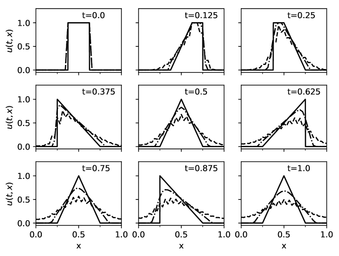
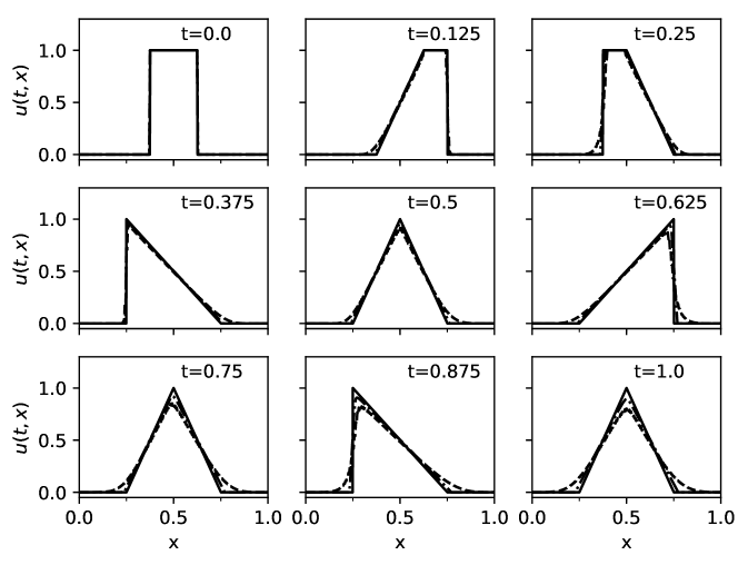
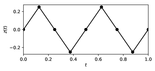
Figure 1. Top and middle: Time series snapshots of the exact (solid line), the Lax–Friedrichs (dashed line) and the Engquist–Osher (dash-dotted line) solutions of Example 3.1 with flux $f(u)=u^{2}/2$ and free resolution parameter $m=2^{3}$ (top $3\times 3$ subfigure) and $m=2^{6}$ (middle $3\times 3$ subfigure). Bottom: The zigzag driving path $z$. The dotted points correspond to the value of $z$ at the respective time series snapshots.

Figure 2 shows snapshots of numerical solutions of the above problem with the only difference being that the flux function here is $f(u)=u^{3}/3$. The free resolution parameter is set to $m=2^{3}$ for the first time series and $m=2^{6}$ for the second one, and an approximate reference solution is computed at resolution $m=2^{12}$ using the Engquist–Osher scheme. We observe that the numerical solutions converge towards the reference solution, and a similar cancellation property as that for $f(u)=u^{2}/2$ seems to hold at the snapshot times $t_{i},t_{j}\geq t_{3}$ displayed here as well.

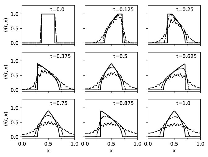
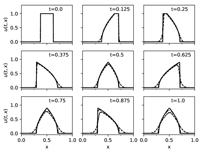
Figure 2. Example 3.1 with flux $f(u)=u^{3}/3$. Approximated reference solution (solid), Lax–Friedrichs (dashed) and Engquist–Osher (dash-dotted). The free resolution parameter is $m=2^{3}$ in the top $3\times 3$ subfigure, and $m=2^{6}$ in the bottom one.

Example 3.2.

We study the problem (3.19) with $T=1$, initial function $u_{0}(x)={\mathbf{1}_{[3/8,5/8]}}(x)$, and flux $f(u)=u^{2}/2$. As driving path $z\in C^{0,\alpha}_{0}([0,1])$ we consider realizations of a fractional Brownian motion (fBM) with Hurst index $\alpha=1/4,1/2$ and $3/4$. We refer to [57] for details on fBM and the circulant embedding algorithm, which we use here to generate realizations on a uniformly spaced mesh $\{\tau_{k}\}_{k=0}^{m}$. The cost of generating $z^{m}$ with this method is ${\mathcal{O}}\!\left(m\log(m)\right)$.

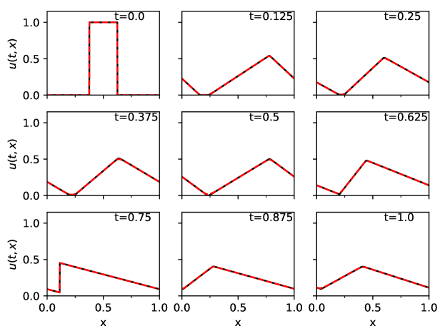
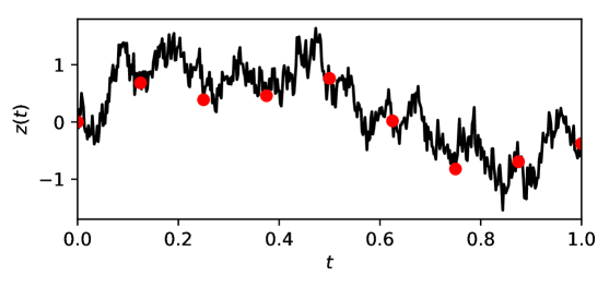
Figure 3. Top: Time series of numerical solutions with $\alpha=0.25$ for Example 3.2. Lax–Friedrichs (red dashed line) and Engquist–Osher (black line). Bottom: The rough path $z$. Red points correspond to the value of $z$ at the respective time series snapshots.

Figures 3,  4, and 5 show time series of “adaptive timestep” numerical solutions for the respective Hurst indices $\alpha=0.25,0.5$ and $0.75$. The free resolution parameter is set to $m=2^{8}$. In Figure 6 we compare the final time numerical solutions $U(1)$ computed with the respective resolutions $m=2^{6}$ and $m=2^{8}$, and with an approximate reference solution computed with resolution $m=2^{10}$ using the more accurate numerical method developed in Section 4.3. A link to the other resolution parameters is obtained through (3.20) and the following property for fBMs: ${\mathbb{E}\mspace{-2.0mu}\left[{\left|z^{m}\right|}_{\mathrm{BV}([0,1])}\right]}={\Theta}\!\left(m^{1-\alpha}\right)$. At resolution $m=2^{8}$, for instance, a typical realization of an fBM sample path yields $\Delta x=2^{-10}$ and $N=2^{12}$ for $\alpha=3/4$; $\Delta x=2^{-12}$ and $N=2^{16}$ for $\alpha=1/2$; and $\Delta x=2^{-14}$ and $N=2^{20}$ for $\alpha=1/4$. We observe that the Engquist–Osher scheme introduces less artificial diffusion and therefore produces more accurate approximations than the the Lax–Friedrichs scheme. (Note that solutions for different values of $\alpha$ are not directly comparable, not least since they are generated from independent fBM sample paths.)

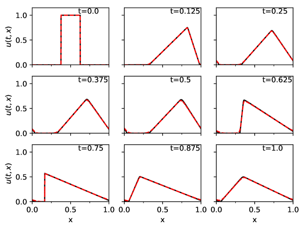
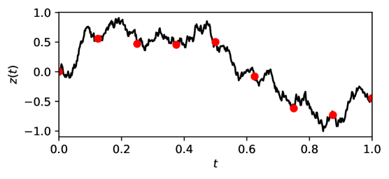
Figure 4. Top: Time series of numerical solutions with $\alpha=0.5$ for Example 3.2. Lax–Friedrichs (red dashed line) and Engquist–Osher (black line). Bottom: The rough path $z$. Red points correspond to the value of $z$ at the respective time series snapshots.

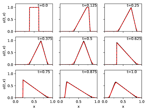
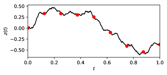
Figure 5. Top: Time series of numerical solutions with $\alpha=0.75$ for Example 3.2. Lax–Friedrichs (red dashed line) and Engquist–Osher (black line). Bottom: The rough path $z$. Red points correspond to the value of $z$ at the respective time series snapshots.

Figure 7 shows the final time approximation error $\|U(1)-u(1)\|_{1}$ as a function of the resolution parameter $m$ for both numerical schemes. The error is averaged over 10 fBM realizations for each of the considered Hurst indices. The convergence rate decreases as $\alpha$ (and thus the regularity of $z$) decreases, but it is consistently orders of magnitude faster than Theorem 3.4’s possible worst case, ${\mathcal{O}}\!\left(m^{-\alpha/2}\right)$.

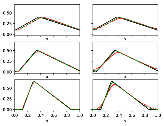
Figure 6. Final time solutions for Example 3.2. Reference solution (black line), numerical solutions at resolutions $m=2^{6}$ (red dashed line) and $m=2^{8}$ (green dash-dot line). Left column: Engquist–Osher scheme, Hurst index $\alpha=0.25,0.5,0.75$ from top to bottom, respectively. Right column: Lax–Friedrichs scheme, Hurst index $\alpha=0.25,0.5,0.75$ from top to bottom, respectively.

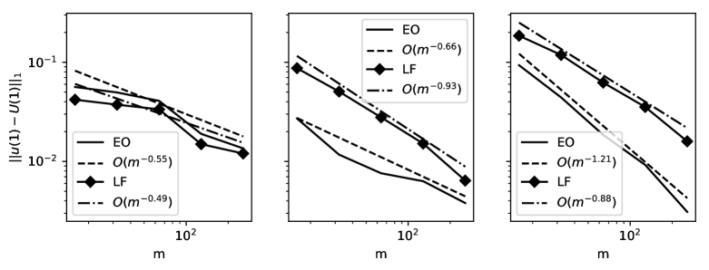
Figure 7. Final time approximation error for Example 3.2. Hurst indices $\alpha=0.25,0.5,0.75$ from left to right, respectively. The abbreviations EO and LF denote respectively the Engquist–Osher and Lax–Friedrichs schemes.

4. Cancellations and improved numerical methods

The numerical experiments in Example 3.2 indicate that the convergence rates obtained in Theorems 3.3 and 3.4 might not be sharp. In view of the more precise adaptive timestep error analysis of the latter theorem, where the factor ${\left|z^{m}\right|}_{BV([0,T])}$ enters, one might suspect that the error bounds could be improved if one were able to identify “rough path oscillations” resulting in “cancellations” in the flux term $\dot{z}^{m}\partial_{x}f(u)$. In this section we identify such oscillatory cancellations for strictly convex flux functions. More precisely, we show that if $f\in C^{2}(\mathbb{R})$ is strictly convex, then the path $z^{m}\in I^{m}_{0}([0,T])$ can be replaced by a “simpler” path $y^{m}\in I^{m}_{0}([0,T])$ (with smaller total variation) such that the solution of (2.1) with path $y^{m}$ coincides with the corresponding solution with path $z^{m}$ at final time $T$ (but not necessarily at earlier times). An efficient numerical method that exploits this property is developed in Section 4.3.

4.1. Preliminaries

Recall that for $\kappa\in\mathbb{R}$, $s\geq 0$, and $v\in(L^{1}\cap BV)(\mathbb{R})$, $\mathcal{S}^{\kappa}(s)v$ denotes the solution at time $t=s$ of

$$\partial_{t}u+\kappa\partial_{x}f(u)=0\quad\text{in}\;(0,\infty)\times\mathbb{R},\qquad u(0,\cdot)=v,$$

so the entropy solution at time $t=T$ of (2.1) with path $z^{m}\in I_{0}([0,T];\{\tau_{j}\}_{j=0}^{m})$ can be expressed by

(4.1) $$u^{m}(T)=\mathcal{S}^{\dot{z}_{m-1}^{m}}(\Delta\tau)\mathcal{S}^{\dot{z}_{m-2}^{m}}(\Delta\tau)\ldots\mathcal{S}^{\dot{z}_{0}^{m}}(\Delta\tau)u_{0}.$$

By a change of variables, the solution mapping can be simplified to only depend on the path increments.

Lemma 4.1.

For any $\Delta\tau>0$, $\kappa\in\mathbb{R}$ and $v\in(L^{1}\cap BV)(\mathbb{R})$, $\mathcal{S}^{\kappa}(\Delta\tau)v$ coincides with the entropy solution at time $t=|\kappa|\Delta\tau$ of

(4.2) $$\partial_{t}\tilde{u}+\operatorname*{sign}\left(\kappa\right)\partial_{x}f(\tilde{u})=0\quad\text{in}\;(0,\infty)\times\mathbb{R},\qquad\tilde{u}(0)=v.$$

Proof.

For $\kappa=0$ the result trivially holds as $\mathcal{S}^{0}(\cdot)=I$. Otherwise, when $|\kappa|>0$, we verify the result by showing that

$$\bar{u}(t,x):=\tilde{u}(t|\kappa|,x)$$

is an entropy solution of

$$\partial_{t}\bar{u}+\kappa\partial_{x}f(\bar{u})=0\quad\text{in}\;(0,\infty)\times\mathbb{R},\qquad\bar{u}(0)=v.$$

Let $\phi\in C^{\infty}_{0}(\mathbb{R}\times\mathbb{R})$ be an arbitrary nonnegative test function and set

(4.3) $$\bar{\phi}(t,x):=\phi(t|\kappa|,x).$$

By construction, for all $c\in\mathbb{R}$, we have

$$\begin{split}&\int_{0}^{|\kappa|\Delta\tau}\int_{\mathbb{R}}|\tilde{u}-c|\partial_{t}\phi+\operatorname*{sign}\left(\tilde{u}-c\right)\operatorname*{sign}\left(\kappa\right)(f(\tilde{u})-f(c))\partial_{x}\phi\,\mathrm{d}x\,\mathrm{d}t\\ &\quad+\int_{\mathbb{R}}|\tilde{u}(0,x)-c|\phi(0,x)-|\tilde{u}(|\kappa|\Delta\tau,x)-c|\phi(|\kappa|\Delta\tau,x)\,\mathrm{d}x\geq 0.\end{split}$$

Making the change of variables $\bar{t}=t/|\kappa|$, we arrive at

$$\begin{split}&\int_{0}^{\Delta\tau}\int_{\mathbb{R}}|\bar{u}-c|(\partial_{t}\phi)\left(\bar{t}|\kappa|,x\right)\\ &\qquad\qquad+\operatorname*{sign}\left(\bar{u}-c\right)\kappa(f(\bar{u})-f(c))(\partial_{x}\phi)\left(\bar{t}|\kappa|,x\right)\,\mathrm{d}x\,\mathrm{d}\bar{t}\\ &\quad+\int_{\mathbb{R}}|\bar{u}(0,x)-c|\bar{\phi}(0,x)-|\bar{u}(\Delta\tau,x)-c|\bar{\phi}(\Delta\tau,x)\,\mathrm{d}x\geq 0.\end{split}$$

Noting that

$$\partial_{t}\phi\left(\bar{t}|\kappa|,x\right)=\partial_{\bar{t}}\phi\left(\bar{t}|\kappa|,x\right)|\kappa|^{-1},$$

it follows that

$$\begin{split}&\int_{0}^{\Delta\tau}\int_{\mathbb{R}}|\bar{u}-c|\partial_{\bar{t}}\bar{\phi}+\operatorname*{sign}\left(\bar{u}-c\right)\kappa(f(\bar{u})-f(c))\partial_{x}\bar{\phi}\,\mathrm{d}x\,\mathrm{d}\bar{t}\\ &\quad+\int_{\mathbb{R}}|\bar{u}(0,x)-c|\bar{\phi}(0,x)-|\bar{u}(\Delta\tau,x)-c|\bar{\phi}(\Delta\tau,x)\,\mathrm{d}x\geq 0.\end{split}$$

In view of (4.3) and the invertibility of the mapping $t\mapsto t|\kappa|$, the above inequality holds for arbitrary nonnegative $\bar{\phi}\in C^{\infty}_{0}(\mathbb{R}\times\mathbb{R})$. ∎

Let $\bar{}\mathcal{S}(\cdot):\mathbb{R}\times(L^{1}\cap BV)(\mathbb{R})\to(L^{1}\cap BV)(\mathbb{R})$ be the solution operator linked to

(4.4) $$\partial_{t}\tilde{u}+\operatorname*{sign}\left(\Delta z\right)\partial_{x}f(\tilde{u})=0\quad\text{in}\;(0,\infty)\times\mathbb{R},\qquad\tilde{u}(0)=v,$$

that is, for $\Delta z\in\mathbb{R}$ and $v\in(L^{1}\cap BV)(\mathbb{R})$, $\bar{}\mathcal{S}(\Delta z)v$ denotes the Kružkov entropy solution at time $t=|\Delta z|$ of (4.4).

Lemma 4.1 implies that for any $z^{m}\in I_{0}([0,T];\{\tau_{j}\}_{j=0}^{m})$, $k\in\{0,1,\ldots,m-1\}$, $s\in[0,\Delta\tau_{k}]$ and $v\in(L^{1}\cap BV)(\mathbb{R})$,

(4.5) $$\mathcal{S}^{\dot{z}^{m}_{k}}(s)v=\bar{}\mathcal{S}(z^{m}(\tau_{k}+s)-z^{m}(\tau_{k}))v.$$

In view of (4.5) and (3.3), the solution of (2.1), for given $u_{0}\in(L^{1}\cap BV)(\mathbb{R})$, $f\in C^{2}(\mathbb{R})$ and driving path $z^{m}\in I^{m}_{0}([0,T])$, can be represented by

(4.6) $$u^{m}(t)=\begin{cases}\bar{}\mathcal{S}(z^{m}(t)-z^{m}(0))u_{0}&\text{if }t\in[0,\tau_{1}],\\ \bar{}\mathcal{S}(z^{m}(t)-z^{m}(\tau_{1}))\bar{}\mathcal{S}(\Delta z_{0}^{m})u_{0}&\text{if }t\in(\tau_{1},\tau_{2}],\\ \cdots\\ \bar{}\mathcal{S}(z^{m}(t)-z^{m}(\tau_{m-1}))\bar{}\mathcal{S}(\Delta{z}_{k-2}^{m})\cdots\bar{}\mathcal{S}(\Delta{z}_{0}^{m})u_{0}&\text{if }t\in(\tau_{m-1},T].\end{cases}$$

To study how an entropy solution depends on the driving path, we introduce the notion “oscillatory cancellations”.

Definition 4.1.

For given $u_{0}\in(L^{1}\cap BV)(\mathbb{R})$, $f\in C^{2}(\mathbb{R})$ and $z^{m}\in I^{m}_{0}([0,T])$, we say there are “oscillatory cancellations” over an interval $[\tau_{k},\tau]\subset[0,T]$, with $k\in\{0,1,\ldots,m-2\}$ and $\tau\in(\tau_{\ell},\tau_{\ell+1}]$ for some $k<\ell\leq m-1$, if it holds that

(4.7) $$\begin{split}u^{m}(\tau)&=\bar{}\mathcal{S}(z^{m}(\tau)-z^{m}(\tau_{\ell}))\cdots\bar{}\mathcal{S}(\Delta z_{k}^{m})u^{m}(\tau_{k})\\ &=\bar{}\mathcal{S}\left(z^{m}(\tau)-z^{m}(\tau_{\ell})+\sum_{j=k}^{\ell-1}\Delta z_{j}^{m}\right)u^{m}(\tau_{k})\\ &=\bar{}\mathcal{S}\left(z^{m}(\tau)-z^{m}(\tau_{k})\right)u^{m}(\tau_{k}).\end{split}$$

Recall from [49, Theorem 2.15] that the solution operator $\bar{}\mathcal{S}$ fulfills the following properties for all $u,v\in(L^{1}\cap BV)(\mathbb{R})$ and $s,t\in\mathbb{R}$:

(4.8) $$\|\bar{S}(s)u-\bar{S}(s)v\|_{L^{1}(\mathbb{R})} \leq\|u-v\|_{L^{1}(\mathbb{R})},$$

(4.9) $$\|\bar{S}(s)u-\bar{S}(t)u\|_{L^{1}(\mathbb{R})} \leq\|f^{\prime}\|_{L^{\infty}}|u|_{\mathrm{BV}(\mathbb{R})}|t-s|,$$

(4.10) $$|\bar{S}(s)u|_{\mathrm{BV}(\mathbb{R})} \leq|u_{0}|_{\mathrm{BV}(\mathbb{R})}.$$

Definition 4.2.

For any $z\in C_{0}([0,T])$, let

(4.11) $$M^{+}[z](t)\mathrel{\vbox{\hbox{\scriptsize.}\hbox{\scriptsize.}}}=\max_{s\in[0,t]}z(s)\quad M^{-}[z](t)\mathrel{\vbox{\hbox{\scriptsize.}\hbox{\scriptsize.}}}=\min_{s\in[0,t]}z(s),\quad t\in[0,T],$$

denote the running max/min functions of $z$.

See Figure 8 for an example illustrating the running max/min functions.

To identify intervals with oscillatory cancellations we make use of the following regularity result:

Corollary 4.2.

Let $u^{m}\in C_{0}([0,T];L^{1}(\mathbb{R}))$ denote the unique entropy solution of (2.1), for given initial data $u_{0}\in(L^{1}\cap BV)(\mathbb{R})$, strictly convex flux $f\in C^{2}(\mathbb{R})$ and driving path $z^{m}\in I^{m}_{0}([0,T])$. If for some $0\leq s_{1}<s_{2}\leq T$,

$$z^{m}(t)\in(M^{-}[z^{m}](s_{1}),M^{+}[z^{m}](s_{1}))\quad\forall t\in(s_{1},s_{2}),$$

then for all $t\in(s_{1},s_{2})$, it holds that $u^{m}(t)\in\mathrm{Lip}(\mathbb{R})$ and

$$\sup_{x\neq y}{\left|\frac{u^{m}(t,y)-u^{m}(t,x)}{y-x}\right|}\leq\frac{\|f^{\prime\prime}\|_{L^{\infty}}^{-1}}{\min\left\{z^{m}(t)-M^{-}[z^{m}](s_{1}),\,M^{+}[z^{m}](s_{1})-z^{m}(t)\right\}},$$

where (as usual) the $L^{\infty}$ is restricted to the interval $\left[-\|u_{0}\|_{\infty},\|u_{0}\|_{\infty}\right]$.

The corollary is a direct consequence of Lemma A.1, $f\in C^{2}(\mathbb{R})$, and the mean-value theorem. We refer to the companion work [44] for an in-depth theoretical treatment of regularity and cancellation properties for (2.1).

Lemma 4.3.

For an $m\geq 2$, let $u^{m}\in C_{0}([0,T];L^{1}(\mathbb{R}))$ denote the unique entropy solution of (2.1) for some initial data $u_{0}\in(L^{1}\cap BV)(\mathbb{R})$, strictly convex $f\in C^{2}(\mathbb{R})$ and driving noise $z^{m}\in I^{m}_{0}([0,T])$. Then property (4.7) holds over an interval $[\tau_{k},\tau]\subset[0,T]$ with $k\in\{0,1,\ldots,m-2\}$ and $\tau\in(\tau_{\ell},\tau_{\ell+1}]$ for some $k<\ell\leq m-1$, if at least one of the following conditions are met:

1. $\dot{z}^{m}(s+)\mathrel{\vbox{\hbox{\scriptsize.}\hbox{\scriptsize.}}}=\lim_{\delta\downarrow 0}\dot{z}^{m}(s+\delta)\geq 0$ for all $s\in[\tau_{k},\tau)$,

2. $\dot{z}^{m}(s+)\leq 0$ for all $s\in[\tau_{k},\tau)$,

3. $z^{m}([\tau_{k},\tau])\subset[M^{-}[z^{m}](\tau_{k}),M^{+}[z^{m}](\tau_{k})]$.

Remark 4.1.

Figure 8 exemplifies the running max/min functions for a piecewise linear function $z^{10}\in I_{0}([0,T];\{\tau_{j}\}_{j=0}^{10})$, where $[\tau_{5},\tau_{7}]$ is of type (i), $[\tau_{7},\tau_{10}=T]$ is of type (ii), and $[\tau_{2},\tau_{5}]$ and $[\tau_{7},\tau]$ with $\tau=\tau_{9}+2\Delta\tau/3$ are of type (iii).

Proof.

(i) & (ii): The condition $\dot{z}^{m}(\cdot+)|_{[\tau_{k},\tau)}\geq 0$ implies that $\Delta z^{m}_{j}\geq 0$ for $j=k,k+1,\ldots,\ell-1$. By the definition of $\bar{}\mathcal{S}$, cf. (4.4),

$$\bar{}\mathcal{S}(z^{m}(\tau)-z^{m}(\tau_{\ell}))\ldots\bar{}\mathcal{S}(\Delta z_{k}^{m})u^{m}(\tau_{k})$$

is equal to the entropy solution at time $t=z^{m}(\tau)-z^{m}(\tau_{\ell})+\sum_{j=k}^{\ell-1}\Delta z^{m}_{j}$ of

$$\partial_{t}\tilde{u}+\operatorname*{sign}\left(z^{m}(\tau)-z^{m}(\tau_{j})\right)\partial_{x}f(\tilde{u})=0,\quad\tilde{u}(0)=u^{m}(\tau_{k}).$$

But, by definition, we also have that

$$\bar{}\mathcal{S}\left(z^{m}(\tau)-z^{m}(\tau_{k})\right)u^{m}(\tau_{k})=\tilde{u}(z^{m}(\tau)-z^{m}(\tau_{k})),$$

and it is clear that (4.7) holds. Part (ii) follows by a similar argument.

(iii): We assume $M^{+}[z^{m}](\tau_{k})-M^{-}[z^{m}](\tau_{k})>0$, as otherwise $\dot{z}^{m}(\cdot+)|_{[\tau_{k},\tau)}=0$ and the cancellation property follows by (i) or (ii).

For a $\delta\in\left(0,(M^{+}[z^{m}](\tau_{k})-M^{-}[z^{m}](\tau_{k}))/2\right)$ we define the approximation path $z^{m,\delta}\in I_{0}([0,T];\{\tau_{j}\}_{j=0}^{m})$ by interpolating the values

$$z^{m,\delta}(\tau_{j})\mathrel{\vbox{\hbox{\scriptsize.}\hbox{\scriptsize.}}}=\begin{cases}z^{m}(\tau_{j})-\delta&\text{if }j\in\{k+1,\ldots,\ell\}\text{ and }z^{m}(\tau_{j})=M^{+}[z^{m}](\tau_{k}),\\ z^{m}(\tau_{j})+\delta&\text{if }j\in\{k+1,\ldots,\ell\}\text{ and }z^{m}(\tau_{j})=M^{-}[z^{m}](\tau_{k}),\\ z^{m}(\tau_{j})&\text{otherwise,}\end{cases}$$

over the set of interpolation points $\{\tau_{j}\}_{j=0}^{m}$. By construction, it then holds that

$$z^{m,\delta}(s)\in(M^{-}[z^{m}](\tau_{k}),M^{+}[z^{m}](\tau_{k})),\qquad\forall s\in(\tau_{k},\tau),$$

(4.12) $$\Big{|}\Delta z^{m,\delta}_{j}-\Delta z^{m}_{j}\Big{|}\leq 2\delta,\quad\text{for all }\quad j\in\{k,k+1,\ldots,\ell-1\},$$

where $\Delta z^{m,\delta}_{j}\mathrel{\vbox{\hbox{\scriptsize.}\hbox{\scriptsize.}}}=z^{m,\delta}(\tau_{j+1})-z^{m,\delta}(\tau_{j})$, and

(4.13) $${\left|z^{m,\delta}(\tau)-z^{m,\delta}(\tau_{\ell})-(z^{m}(\tau)-z^{m}(\tau_{\ell}))\right|}\leq 2{\left|z^{m,\delta}(\tau_{\ell})-z^{m}(\tau_{\ell})\right|}\leq 2\delta.$$

Let $u^{m,\delta}$ denote the solution of (2.1) with driving path $z^{m,\delta}$ and the same initial data $u_{0}$ and flux $f$ as the solution $u^{m}$. Since $z^{m,\delta}|_{[0,\tau_{k}]}=z^{m}|_{[0,\tau_{k}]}$, (4.4) implies

$$u^{m,\delta}(t)=\begin{cases}u^{m}(t)&\text{if }t\leq\tau_{k},\\ \bar{}\mathcal{S}(z^{m,\delta}(t)-z^{m}(\tau_{k}))u^{m}(\tau_{k})&\text{if }t\in(\tau_{k},\tau_{k+1}],\\ \cdots\\ \bar{}\mathcal{S}(z^{m,\delta}(t)-z^{m,\delta}(\tau_{\ell}))\cdots\bar{}\mathcal{S}(\Delta z^{m,\delta}_{k})u^{m}(\tau_{k}),&\text{if }t\in(\tau_{\ell},\tau].\end{cases}$$

By Corollary 4.2 it holds that $u^{m,\delta}(s)\in\mathrm{Lip}(\mathbb{R})$ for all $s\in(\tau_{k},\tau)$. Consequently, $u^{m,\delta}|_{(\tau_{k},\tau)\times\mathbb{R}}$ is a classical solution that is time invertible, as it can be obtained by the method of characteristics. By (4.9), we further obtain that

$$\begin{split}&\bar{}\mathcal{S}\left(z^{m,\delta}(\tau)-z^{m,\delta}(\tau_{\ell})\right)\cdots\bar{}\mathcal{S}(\Delta z^{m,\delta}_{k})u^{m}(\tau_{k})\\ &=\lim_{\epsilon\downarrow 0}\Big{[}\bar{}\mathcal{S}\left(z^{m,\delta}(\tau)-z^{m,\delta}(\tau-\epsilon)\right)\bar{}\mathcal{S}\left(z^{m,\delta}(\tau-\epsilon))-z^{m,\delta}(\tau_{\ell})\right)\bar{}\mathcal{S}(\Delta z^{m,\delta}_{\ell-1})\cdots\\ &\quad\quad\bar{}\mathcal{S}(\Delta z^{m,\delta}_{k+1})\bar{}\mathcal{S}\left(z^{m,\delta}(\tau_{k+1})-z^{m,\delta}(\tau_{k}+\epsilon)\right)\bar{}\mathcal{S}\left(z^{m,\delta}(\tau_{k}+\epsilon)-z^{m,\delta}(\tau_{k})\right)u^{m}(\tau_{k})\Big{]}\\ &=\lim_{\epsilon\downarrow 0}\Big{[}\bar{}\mathcal{S}\left(z^{m,\delta}(\tau)-z^{m,\delta}(\tau-\epsilon)\right)\bar{}\mathcal{S}\left(z^{m,\delta}(\tau-\epsilon))-z^{m,\delta}(\tau_{k}+\epsilon)\right)\\ &\qquad\qquad\bar{}\mathcal{S}\left(z^{m,\delta}(\tau_{k}+\epsilon)-z^{m,\delta}(\tau_{k})\right)u^{m}(\tau_{k})\Big{]}\\ &=\bar{}\mathcal{S}\left(z^{m,\delta}(\tau))-z^{m,\delta}(\tau_{k})\right)u^{m}(\tau_{k}).\end{split}$$

By (4.8), (4.9), (4.10), (4.12) and (4.13),

$$\begin{split}&{\left\|\bar{}\mathcal{S}\left(z^{m}(\tau)-z^{m}(\tau_{\ell})\right)\cdots\bar{}\mathcal{S}(\Delta z_{k}^{m})u^{m}(\tau_{k})-\bar{}\mathcal{S}\left(z^{m,\delta}(\tau)-z^{m,\delta}(\tau_{k})\right)u^{m}(\tau_{k})\right\|}_{L^{1}}\\ &={\left\|\left[\bar{}\mathcal{S}\left(z^{m}(\tau)-z^{m}(\tau_{\ell})\right)\cdots\bar{}\mathcal{S}(\Delta z_{k}^{m})-\bar{}\mathcal{S}\left(z^{m,\delta}(\tau)-z^{m,\delta}(\tau_{\ell})\right)\cdots\bar{}\mathcal{S}(\Delta z^{m,\delta}_{k})\right]u^{m}(\tau_{k})\right\|}_{L^{1}}\\ &\leq{\left\|\Big{[}\bar{}\mathcal{S}\left(z^{m}(\tau)-z^{m}(\tau_{\ell})\right)-\bar{}\mathcal{S}\left(z^{m,\delta}(\tau)-z^{m,\delta}(\tau_{\ell})\right)\Big{]}\bar{}\mathcal{S}(\Delta z_{\ell-1}^{m})\cdots\bar{}\mathcal{S}(\Delta z_{k}^{m})u^{m}(\tau_{k})\right\|}_{L^{1}}\\ &+{\left\|\bar{}\mathcal{S}\left(z^{m,\delta}(\tau)-z^{m,\delta}(\tau_{\ell})\right)\left[\bar{}\mathcal{S}(\Delta z_{\ell-1}^{m})-\bar{}\mathcal{S}(\Delta z_{\ell-1}^{m,\delta})\right]\bar{}\mathcal{S}(\Delta z_{\ell-2}^{m})\cdots\bar{}\mathcal{S}(\Delta z_{k}^{m})u^{m}(\tau_{k})\right\|}_{L^{1}}\\ &+\cdots+{\left\|\bar{}\mathcal{S}\left(z^{m,\delta}(\tau)-z^{m,\delta}(\tau_{\ell})\right)\cdots\bar{}\mathcal{S}(\Delta z_{k+1}^{m,\delta})\left[\bar{}\mathcal{S}(\Delta z_{k}^{m})-\bar{}\mathcal{S}(\Delta z_{k}^{m,\delta})\right]u^{m}(\tau_{k})\right\|}_{L^{1}}\\ &\leq 2\delta(\ell+1-k)\|f^{\prime}\|_{\infty}|u_{0}|_{\mathrm{BV}}.\end{split}$$

Taking the limit $\delta\downarrow 0$, shows that  (4.7) holds in $L^{1}(\mathbb{R})$-sense. ∎

4.2. The oscillating running max and min functions

Lemma 4.3 identifies a class of intervals over which an entropy solution with driving path $z^{m}\in I^{m}_{0}([0,T])$ experience “oscillatory cancellations”. In this section we construct an alternative driving path from $z^{m}$ that is free of Lemma 4.3’s type (iii) “oscillatory cancellations”, has lower total variation than $z^{m}$, and (under some assumptions) produces the same entropy solution at the final time as $z^{m}$ does. The further removal of type (i), (ii) “oscillatory cancellations” is postponed to Section 4.3.

Definition 4.3.

For any $z\in C_{0}([0,T])$, we define the monotonically increasing functions $A^{+}[z],A^{-}[z]:[0,T]\to[0,T]$ by

$$A^{+}[z](t) :=\min\{s\in[0,t]\,|\,z(s)=M^{+}[z](t)\},$$

$$A^{-}[z](t) :=\min\{s\in[0,t]\,|\,z(s)=M^{-}[z](t)\},$$

and the monotonically increasing càdlàg functions $\bar{A}^{+}[z],\bar{A}^{-}[z]:[0,T]\to[0,T]$ by

(4.14) $$\begin{split}\bar{A}^{+}[z](t)&:=\begin{cases}\lim\limits_{\delta\downarrow 0}A^{+}[z](t+\delta)&\text{if}\quad t\in[0,T),\\ A^{+}[z](T)&\text{if}\quad t=T,\end{cases}\\ \bar{A}^{-}[z](t)&:=\begin{cases}\lim\limits_{\delta\downarrow 0}A^{-}[z](t+\delta)&\text{if}\quad t\in[0,T),\\ A^{-}[z](T)&\text{if}\quad t=T.\end{cases}\end{split}$$

For a given set of points

$$0=\tau_{0}<\tau_{1}<\ldots<\tau_{m}=T,$$

and $z^{m}=\mathcal{I}[z](\cdot;\{\tau_{k}\}_{k=0}^{m})$, define

$$A^{\pm}[z^{m}]:=\bar{A}^{+}[z^{m}](\{\tau_{k}\}_{k=0}^{m})\cup\bar{A}^{-}[z^{m}](\{\tau_{k}\}_{k=0}^{m})\subset\{\tau_{k}\}_{j=0}^{m}.$$

The set inclusion $A^{\pm}[z^{m}]\subset\{\tau_{k}\}_{j=0}^{m}$ is verified in Lemma 4.4.

Note that $0\in A^{\pm}[z^{m}]$, and let $\{\tau_{j(k)}\}_{k=0}^{\bar{m}}=A^{\pm}[z^{m}]\cup\{T\}$, with $0=j(0)<\cdots<j(\bar{m})=m$, represent the subsequence of interpolation points in ascending order. The operator $\overline{\operatorname{orm}}:C_{0}([0,T])\to I^{m}_{0}([0,T])$ is defined by

(4.15) $$\begin{split}&\overline{\operatorname{orm}}[z](t;\{\tau_{j(k)}\}_{k=0}^{\bar{m}})\\ &=\sum_{k=0}^{\bar{m}-1}{\mathbf{1}_{t\in(\tau_{j(k)},\tau_{j(k+1)}]}}\left(z(\tau_{j(k)})+\left(z(\tau_{j(k+1)})-z(\tau_{j(k)})\right)\frac{t-\tau_{j(k)}}{\tau_{j(k+1)}-\tau_{j(k)}}\right).\end{split}$$

We refer to $\overline{\operatorname{orm}}[z]\left(\cdot;\{\tau_{j(k)}\}_{k=0}^{\bar{m}}\right)$ as the piecewise linear oscillating running max/min (orm) function of $z$, and frequently use the shorthand $\overline{\operatorname{orm}}_{m}[z]=\overline{\operatorname{orm}}[z]\left(\cdot;\{\tau_{j(k)}\}_{k=0}^{\bar{m}}\right)$ (if no confusion is possible).

See Figure 8 for an example illustrating $\bar{A}^{+}[z^{m}]$, $\bar{A}^{-}[z^{m}]$, and $\overline{\operatorname{orm}}_{m}[z]$.

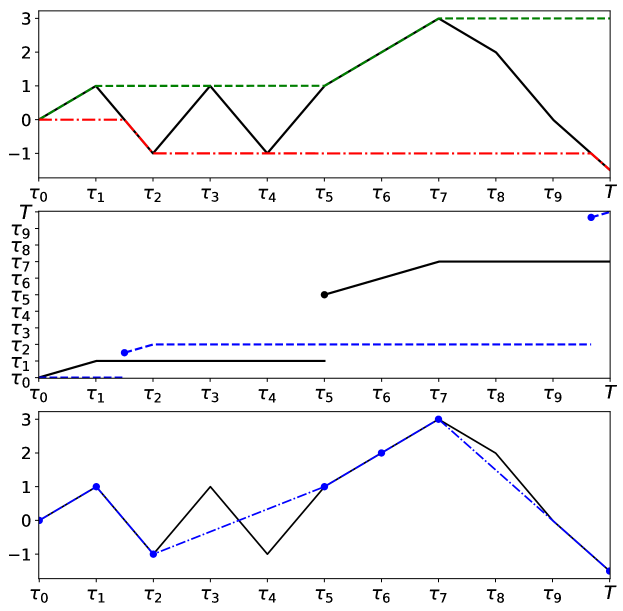
Figure 8. Top: The piecewise linear path $z^{m}\in I_{0}([0,T];\{\tau_{j}\}_{j=0}^{m})$ with $m=10$ (black line) and the associated running maximum $M^{+}[z^{m}]$ (green dashed line) and running minimum $M^{-}[z^{m}]$ (red dash-dotted line). Middle: $\bar{A}^{+}[z^{m}]$ (black line) and $\bar{A}^{-}[z^{m}]$ (blue dashed line). Black and blue dots illustrate that the respective functions are right-continuous at jump discontinuities. Bottom: The piecewise linear path $z^{m}$ (black line) and the associated $\overline{\operatorname{orm}}_{m}[z]$ (blue dash-dotted line). Blue dots mark the value of $\overline{\operatorname{orm}}_{m}[z]$ at its interpolation points $\{\tau_{j(k)}\}_{k=0}^{m}$.

For later reference we collect some properties of $\bar{A}^{\pm}[z]$ in a lemma.

Lemma 4.4.

Assume that $z\in C_{0}([0,T])$. Then, for all $t\in[0,T]$,

$$\max(\bar{A}^{+}[z],\bar{A}^{-}[z])(t)\leq t,$$

(4.16) $$\begin{split}z(\bar{A}^{+}[z](t))&=M^{+}[z](\bar{A}^{+}[z](t))=M^{+}[z](t),\\ z(\bar{A}^{-}[z](t))&=M^{-}[z](\bar{A}^{-}[z](t))=M^{-}[z](t),\end{split}$$

(4.17) $$\bar{A}^{+}[z](\bar{A}^{+}[z](t))=\bar{A}^{+}[z](t),\quad\bar{A}^{-}[z](\bar{A}^{-}[z](t))=\bar{A}^{-}[z](t).$$

Furthermore, for any set of points that satisfies

$$0=\tau_{0}<\tau_{1}<\ldots<\tau_{m}=T,\qquad m\geq 2,$$

and $z^{m}=\mathcal{I}[z](\cdot;\{\tau_{k}\}_{k=0}^{m})$, it holds that

(4.18) $$A^{\pm}[z^{m}]\subset\{\tau_{k}\}_{k=0}^{m}$$

and

(4.19) $$\tau=\max\left\{\bar{A}^{+}[z],\bar{A}^{-}[z]\right\}(\tau)\quad\text{ for all $\tau\in A^{\pm}[z^{m}]$.}$$

Proof.

By Definition 4.3,

$$\max(\bar{A}^{+}[z],\bar{A}^{-}[z])(t)=\lim_{\delta\downarrow 0}\max(A^{+}[z],A^{-}[z])(t+\delta)\leq\lim_{\delta\downarrow 0}(t+\delta)=t.$$

To verify (4.16), $z\in C_{0}([0,T])$ implies that $M^{+}[z]\in C_{0}([0,T])$,

$$\begin{split}z(\bar{A}^{+}[z](t))&=z(\lim_{\delta\downarrow 0}A^{+}[z](t+\delta))\\ &=\lim_{\delta\downarrow 0}z(A^{+}[z](t+\delta))\\ &=\lim_{\delta\downarrow 0}M^{+}[z](t+\delta)\\ &=M^{+}[z](t),\end{split}$$

and

$$\begin{split}M^{+}[z](\bar{A}^{+}[z](t))&=M^{+}[z](\lim_{\delta\downarrow 0}A^{+}[z](t+\delta))\\ &=\lim_{\delta\downarrow 0}M^{+}[z](A^{+}[z](t+\delta))\\ &=\lim_{\delta\downarrow 0}M^{+}[z](t+\delta)\\ &=M^{+}[z](t).\end{split}$$

The second line of (4.16) follows by a similar argument.

To verify (4.17), we begin by noting that for all $t\in[0,T]$,

(4.20) $$\begin{split}A^{+}[z](A^{+}[z](t))&=\min\{s\in[0,A^{+}[z](t)]\mid z(s)=M^{+}[z](A^{+}[z](t))\}\\ &=\min\{s\in[0,A^{+}[z](t)]\mid z(s)=M^{+}[z](t)\}\\ &=A^{+}[z](t).\end{split}$$

By writing

$$B_{1}^{+}[z]=\{t\in[0,T)\mid\lim_{\delta\downarrow 0}A^{+}[z](t+\delta)-A^{+}[z](t)=0\}\cup\{T\}$$

and

$$B_{2}^{+}[z]=\{t\in[0,T)\mid\lim_{\delta\downarrow 0}A^{+}[z](t+\delta)-A^{+}[z](t)>0\},$$

we see that for all $t\in B_{1}^{+}[z]$, $\bar{A}^{+}[z](t)=A^{+}[z](t)$. Hence,

$$\bar{A}^{+}[z](\bar{A}^{+}[z](t))\leq\bar{A}^{+}[z](t)=A^{+}[z](t)$$

and since $\bar{A}^{+}[z]\geq A^{+}[z]$,

$$\bar{A}^{+}[z](\bar{A}^{+}[z](t))\geq A^{+}[z](A^{+}[z](t))=A^{+}[z](t).$$

We conclude that

$$\bar{A}^{+}[z](\bar{A}^{+}[z](t))=A^{+}[z](t)=\bar{A}^{+}[z](t)\quad\forall t\in B_{1}^{+}[z].$$

We claim that for all $t\in B_{2}^{+}[z]$ and $\delta\in(0,T-t)$, it holds that $A^{+}[z](t+\delta)>t$; supposing otherwise, (4.20) and the monotonicity (increasing) of $A^{+}[z]$ leads to the following contradiction

$$A^{+}[z](t+\delta)-A^{+}[z](t)=A^{+}[z](A^{+}[z](t+\delta))-A^{+}[z](t)\leq 0.$$

Hence, for all $t\in B_{2}^{+}[z]$, it follows by the preceding observation and $\bar{A}^{+}[z](t)\leq t$ that $\bar{A}^{+}[z](\bar{A}^{+}[z](t))=\bar{A}^{+}[z](t)$. The equality $\bar{A}^{-}[z](\bar{A}^{-}[z](t))=\bar{A}^{-}[z](t)$ can be verified by a similar argument.

To verify (4.18), observe that since $z^{m}$ is piecewise linear, it holds that

$$A^{+}[z^{m}](\{\tau_{k}\}_{k=0}^{m})\cup A^{-}[z^{m}](\{\tau_{k}\}_{k=0}^{m})\subset\{\tau_{k}\}_{r=0}^{m},$$

and for all $k\in\{0,1,\ldots,m\}$,

$$\bar{A}^{+}[z^{m}](\tau_{k})=\begin{cases}A^{+}[z^{m}](\tau_{k})&\text{if }\tau_{k}\in B_{1}^{+}[z^{m}],\\ \tau_{k}&\text{if }\tau_{k}\in B_{2}^{+}[z^{m}],\end{cases}$$

and

$$\bar{A}^{-}[z^{m}](\tau_{k})=\begin{cases}A^{-}[z^{m}](\tau_{k})&\text{if }\tau_{k}\in B_{1}^{-}[z^{m}],\\ \tau_{k}&\text{if }\tau_{k}\in B_{2}^{-}[z^{m}],\end{cases}$$

where

$$B_{1}^{-}[z^{m}]=\{t\in[0,T)\mid\lim_{\delta\downarrow 0}A^{-}[z^{m}](t+\delta)-A^{-}[z^{m}](t)=0\}\cup\{T\}$$

and

$$B_{2}^{-}[z]=\{t\in[0,T)\mid\lim_{\delta\downarrow 0}A^{-}[z^{m}](t+\delta)-A^{-}[z^{m}](t)>0\}.$$

To verify (4.19), equation (4.17) implies that for any $\tau\in\bar{A}^{+}[z^{m}](\{\tau_{k}\}_{k=0}^{m})$,

$$\bar{A}^{+}[z^{m}](\tau)=\tau\quad\text{and}\quad\bar{A}^{-}[z^{m}](\tau)\leq\tau,$$

and for any $\tau\in\bar{A}^{-}[z^{m}](\{\tau_{k}\}_{k=0}^{m})$,

$$\bar{A}^{-}[z^{m}](\tau)=\tau\quad\text{and}\quad\bar{A}^{+}[z^{m}](\tau)\leq\tau.$$

∎

To extend the solution representation (4.6) to paths with jump discontinuities and to study asymptotic properties of $\overline{\operatorname{orm}}_{m}$ for $m\to\infty$, we introduce

Definition 4.4.

Let $\mathcal{D}([0,T])$ denote the space of càdlàg functions $g:[0,T]\to\mathbb{R}$. For some $m\geq 2$, let $\{\tau_{k}\}_{k=0}^{m}$ be a set of points with $0=\tau_{0}<\tau_{1}<\ldots<\tau_{m}=T$. Given $f\in C^{2}(\mathbb{R})$, $u_{0}\in(L^{1}\cap BV)(\mathbb{R})$ and $y\in\mathcal{D}([0,T])$, we define

(4.21) $$v(\tau_{k};y,\{\tau_{k}\}_{k=0}^{m})\mathrel{\vbox{\hbox{\scriptsize.}\hbox{\scriptsize.}}}=\begin{cases}u_{0}&\text{if }k=0\\ \bar{}\mathcal{S}(\Delta y_{k-1})\bar{}\mathcal{S}(\Delta{y}_{k-2})\ldots\bar{}\mathcal{S}(\Delta{y}_{0})u_{0}&\text{if }k\in\{1,\ldots,m\},\end{cases}$$

where $\Delta y_{k}=y(\tau_{k+1})-y(\tau_{k})$.

Note that for any $f\in C^{2}(\mathbb{R})$, $u_{0}\in(L^{1}\cap BV)(\mathbb{R})$, set of points

$$0=\tau_{0}<\tau_{1}<\ldots<\tau_{m}=T,\qquad m\geq 2,$$

and $y\in\mathcal{D}([0,T])$, it holds by (4.8), (4.10) and induction that

$$\|v(\tau_{k};y,\{\tau_{r}\}_{r=0}^{m})\|_{L^{1}}\leq\|u_{0}\|_{L^{1}}\qquad{\left|v(\tau_{k};y,\{\tau_{r}\}_{r=0}^{m})\right|}_{\mathrm{BV}}\leq|u_{0}|_{\mathrm{BV}}\quad\forall k\leq m.$$

Moreover, cf. (4.6),

$$v(T;z,\{\tau_{k}\}_{k=0}^{m})=v(T;\mathcal{I}^{m}[z],\{\tau_{k}\}_{k=0}^{m})=u^{m}(T),\quad z\in C_{0}([0,T]).$$

The next theorem shows that if the flux is strictly convex, then the driving paths $\mathcal{I}^{m}[z]$ and $\overline{\operatorname{orm}}_{m}[z]$ produce the same entropy solution at final time.

Theorem 4.5.

Assume that $f\in C^{2}(\mathbb{R})$ is strictly convex, $u_{0}\in(L^{1}\cap BV)(\mathbb{R})$ and $z\in C_{0}([0,T])$. For some $m\geq 2$, let $\{\tau_{k}\}_{k=0}^{m}$ denote a set of points satisfying $0=\tau_{0}<\tau_{1}<\ldots<\tau_{m}=T$, $z^{m}=\mathcal{I}^{m}[z]$, and let

$$0=\tau_{j(0)}<\tau_{j(1)}<\ldots<\tau_{j(\bar{m})}=T$$

denote the associated interpolation points of $\,\overline{\operatorname{orm}}[z]\left(\cdot;\{\tau_{j(k)}\}_{j=0}^{\bar{m}}\right)$, cf. Definition 4.3. Then

$$v(T;\overline{\operatorname{orm}}_{m}[z],\{\tau_{j(k)}\}_{k=0}^{\bar{m}})=v(T;\overline{\operatorname{orm}}_{m}[z],\{\tau_{k}\}_{k=0}^{m})=v(T;z^{m},\{\tau_{k}\}_{k=0}^{m}).$$

Proof.

Recall from the solution representations (4.6) and (4.21) that

$$v(T;z^{m},\{\tau_{k}\}_{k=0}^{m})=u^{m}(T)=\bar{}\mathcal{S}(\Delta z^{m}_{m-1})\cdots\bar{}\mathcal{S}(\Delta z^{m}_{0})u_{0}.$$

By writing $y^{m}=\overline{\operatorname{orm}}_{m}[z]$ and introducing the shorthand

$$v^{m}(\tau_{k})\mathrel{\vbox{\hbox{\scriptsize.}\hbox{\scriptsize.}}}=v(\tau_{k};y^{m},\{\tau_{r}\}_{r=0}^{m}),\quad\forall k\in\{0,1,\ldots,m\},$$

we have by (4.21),

$$v^{m}(T)=\bar{}\mathcal{S}(\Delta y^{m}_{m-1})\ldots\bar{}\mathcal{S}(\Delta y^{m}_{0})u_{0}.$$

For any $k\in\{0,\ldots,\bar{m}-1\}$, $y^{m}|_{[\tau_{j(k)},\tau_{j(k+1)}]}$ is a linear function. Therefore, either

$$\dot{y}^{m}(s+)\geq 0,\quad\forall s\in[\tau_{j(k)},\tau_{j(k+1)})$$

or

$$\dot{y}^{m}(s+)\leq 0,\quad\forall s\in[\tau_{j(k)},\tau_{j(k+1)}),$$

for any $k\in\{0,\ldots,\bar{m}-1\}$, and Lemma 4.3 and $y^{m}|_{A_{\tau}^{\pm}[z^{m}]\cup\{T\}}=z^{m}|_{A_{\tau}^{\pm}[z^{m}]\cup\{T\}}$, cf. (4.15), yield

$$\begin{split}v^{m}(T)&=\bar{}\mathcal{S}\left(y^{m}(\tau_{j(\bar{m})})-y^{m}(\tau_{j(\bar{m}-1)})\right)\ldots\bar{}\mathcal{S}\left(y^{m}(\tau_{j(1)})-y^{m}(\tau_{j(0)})\right)u_{0}\\ &=\bar{}\mathcal{S}\left(z^{m}(\tau_{j(\bar{m})})-z^{m}(\tau_{j(\bar{m}-1)})\right)\ldots\bar{}\mathcal{S}\left(z^{m}(\tau_{j(1)})-z^{m}(\tau_{j(0)})\right)u_{0}.\end{split}$$

Assume $\bar{m}>1$ (otherwise $z^{m}|_{[0,\tau_{m-1}]}=0$ and the lemma trivially holds). We claim that for all $k\in\{0,\ldots,\bar{m}-1\}$ such that $j(k+1)-j(k)\geq 2$,

(4.22) $$\begin{split}\bar{}\mathcal{S}\left(z^{m}(\tau_{j(k+1)})-z^{m}(\tau_{j(k)}))u^{m}(\tau_{j(k)}\right)&=\bar{}\mathcal{S}\left(\Delta z^{m}_{j(k+1)-1}\right)\ldots\bar{}\mathcal{S}\left(\Delta z^{m}_{j(k)}\right)u^{m}(\tau_{j(k)})\\ &=u^{m}(\tau_{j(k+1)}).\end{split}$$

Define

$$k_{1}=\min\left\{k\in\{0,\ldots,\bar{m}-1\}\big{|}j(k+1)-j(k)\geq 2\right\}\cup\left\{\bar{m}\right\}.$$

Then, since $j(k+1)-j(k)=1$ for all $k<k_{1}$, it follows from the solution representations (4.6) and (4.21) that $v^{m}(\tau_{j(k_{1})})=u^{m}(\tau_{j(k_{1})})$. If $k_{1}=\bar{m}$, we have $v^{m}(T)=u^{m}(T)$. Otherwise, if $k_{1}<\bar{m}$, assumption (4.22) implies that $v^{m}(\tau_{j(k_{1}+1)})=u^{m}(\tau_{j(k_{1}+1)})$. Let

$$k_{2}=\min\left\{k\in\{k_{1}+1,\ldots,\bar{m}-1\}|j(k+1)-j(k)\geq 2\right\}\cup\{\bar{m}\},$$

and argue as above to conclude that if $k_{2}=\bar{m}$, then $v^{m}(T)=u^{m}(T)$, and otherwise, $v^{m}(\tau_{j(k_{2}+1)})=u^{m}(\tau_{j(k_{2}+1)})$. The lemma follows by induction once we have verified the claim (4.22).

Suppose $k\in\{0,\ldots,\bar{m}-1\}$ satisfies $j(k+1)-j(k)\geq 2$. Consider two cases: $\tau_{j(k+1)}\notin A^{\pm}[z^{m}]$ and $\tau_{j(k+1)}\in A^{\pm}[z^{m}]$.

The case $\tau_{j(k+1)}\notin A^{\pm}[z^{m}]$ is only possible if $k=\bar{m}-1$, i.e., if $\tau_{j(k+1)}=T$. Then

$$z^{m}(\tau_{\ell})\in[M^{-}[z^{m}](\tau_{j(k)}),M^{+}[z^{m}](\tau_{j(k)})],\quad\forall\ell\in\{j(\bar{m}-1),j(\bar{m}-1)+1,\ldots,j(\bar{m})\},$$

which implies that

$$z^{m}([\tau_{j(k)},T])\subset[M^{-}[z^{m}](\tau_{j(k)}),M^{+}[z^{m}](\tau_{j(k)})],$$

and (4.22) follows by Lemma 4.3.

For the second case; $\tau_{j(k+1)}\in A^{\pm}[z^{m}]$, then

$$z^{m}(\tau_{\ell})\in[M^{-}[z^{m}](\tau_{j(k)}),M^{+}[z^{m}](\tau_{j(k)})],\quad\forall\ell\in\{j(k),j(k)+1,\ldots,j(k+1)-1\},$$

and there exists a unique $\tau\in(\tau_{j(k+1)-1},\tau_{j(k+1)}]$ such that

(4.23) $$\begin{split}&z^{m}([\tau_{j(k)},\tau])\subset[M^{-}[z^{m}](\tau_{j(k)}),M^{+}[z^{m}](\tau_{j(k)})],\\ &\tau\in\{\bar{A}^{+}[z^{m}](\tau),\bar{A}^{-}[z^{m}](\tau)\}.\end{split}$$

To show (4.23), if $z^{m}(\tau_{j(k+1)})\in[M^{-}[z^{m}](\tau_{j(k)}),M^{+}[z^{m}](\tau_{j(k)})]$ then $\tau=\tau_{j(k+1)}$. Otherwise, if $z^{m}(\tau_{j(k+1)})\notin[M^{-}[z^{m}](\tau_{j(k)}),M^{+}[z^{m}](\tau_{j(k)})]$, then
$z^{m}(\tau_{j(k+1)-1})\in[M^{-}[z^{m}](\tau_{j(k)}),M^{+}[z^{m}](\tau_{j(k)})]$ implies that $|\Delta z^{m}_{j(k+1)-1}|>0$. This observation and $\tau_{j(k+1)-1}\notin A^{\pm}[z^{m}]$ verifies statement (4.23).

By (4.23) and Lemma 4.3,

$$\begin{split}&\bar{}\mathcal{S}(\Delta z^{m}_{j(k+1)-1})\ldots\bar{}\mathcal{S}(\Delta z^{m}_{j(k)})u^{m}(\tau_{j(k)})\\ &=\bar{}\mathcal{S}\left(\Delta z^{m}(\tau_{j(k+1)})-z^{m}(\tau)\right)\bar{}\mathcal{S}\left(z^{m}(\tau)-z^{m}(\tau_{j(k+1)-1})\right)\ldots\bar{}\mathcal{S}(\Delta z^{m}_{j(k)})u^{m}(\tau_{j(k)})\\ &=\bar{}\mathcal{S}(\Delta z^{m}(\tau_{j(k+1)})-z^{m}(\tau))\bar{}\mathcal{S}(z^{m}(\tau)-z^{m}(\tau_{j(k)}))u^{m}(\tau_{j(k)}).\end{split}$$

If $\tau_{j(k+1)}=\bar{A}^{+}[z^{m}](\tau_{j(k+1)})$, then it must hold that $\Delta z^{m}_{j(k+1)-1}\geq 0$, hence, $z^{m}(\tau_{j(k+1)})-z^{m}(\tau)\geq 0$. The former inequality and $\tau\in\{\bar{A}^{+}[z^{m}](\tau),\bar{A}^{-}[z^{m}](\tau)\}$ imply that $z^{m}(\tau)=M^{+}[z^{m}](\tau)$, so that also $z^{m}(\tau)-z^{m}(\tau_{j(k)})\geq 0$. If, on the other hand, $\tau_{j(k+1)}=\bar{A}^{-}[z^{m}](\tau_{j(k+1)})$, then a similar argument yields

$$z^{m}(\tau_{j(k+1)})-z^{m}(\tau)\leq 0\quad\text{and}\quad z^{m}(\tau)-z^{m}(\tau_{j(k)})\leq 0.$$

We conclude from the above that if $\tau_{j(k+1)}\in A^{\pm}[z^{m}]$, then

$$(z^{m}(\tau_{j(k+1)})-z^{m}(\tau))(z^{m}(\tau)-z^{m}(\tau_{j(k)}))\geq 0.$$

Since both increments either are non-negative or non-positive,

$$\bar{}\mathcal{S}\left(z^{m}(\tau_{j(k+1)})-z^{m}(\tau)\right)\bar{}\mathcal{S}\left(z^{m}(\tau)-z^{m}(\tau_{j(k)})\right)u^{m}(\tau_{j(k)})$$

equals the unique entropy solution at time

$$t={\left|z^{m}(\tau_{j(k+1)})-z^{m}(\tau)+(z^{m}(\tau)-z^{m}(\tau_{j(k)}))\right|}={\left|z^{m}(\tau_{j(k+1)})-z^{m}(\tau_{j(k)})\right|}$$

of

$$\partial_{t}\tilde{u}+\operatorname*{sign}\left(z^{m}(\tau_{j(k+1)})-z^{m}(\tau_{j(k)})\right)\partial_{x}f(\tilde{u})=0,\quad\tilde{u}(0)=u^{m}(\tau_{j(k)}),$$

cf. (4.4). However,

$$\bar{}\mathcal{S}(z^{m}(\tau_{j(k+1)})-z^{m}(\tau_{j(k)}))u^{m}(\tau_{j(k)})$$

also equals $\tilde{u}(|z^{m}(\tau_{j(k+1)})-z^{m}(\tau_{j(k)})|)$. Hence,

$$\begin{split}u^{m}(\tau_{j(k+1)})&=\bar{}\mathcal{S}(\Delta z^{m}_{j(k+1)-1})\cdots\bar{}\mathcal{S}(\Delta z^{m}_{j(k)})u^{m}(\tau_{j(k)})\\ &=\bar{}\mathcal{S}(\Delta z^{m}(\tau_{j(k+1)})-z^{m}(\tau))\bar{}\mathcal{S}(z^{m}(\tau)-z^{m}(\tau_{j(k)}))u^{m}(\tau_{j(k)})\\ &=\bar{}\mathcal{S}(z^{m}(\tau_{j(k+1)})-z^{m}(\tau_{j(k)}))u^{m}(\tau_{j(k)}).\end{split}$$

∎

The operator $\overline{\operatorname{orm}}_{m}:C_{0}([0,T])\to I_{0}([0,T];\{\tau_{j}\}_{j=0}^{m})$ introduced in Definition 4.3 maps every driving path $z\in C_{0}([0,T])$ to a less oscillatory driving path $y^{m}=\overline{\operatorname{orm}}_{m}[z]$. In Theorem 4.5 it is shown that, provided $u_{0}\in(L^{1}\cap BV)(\mathbb{R})$ and $f\in C^{2}(\mathbb{R})$ is strictly convex, the paths $z^{m}=\mathcal{I}^{m}[z]$ and $\overline{\operatorname{orm}}_{m}[z]$ are equivalent in the sense of preserving final time solutions:

$$v(T;\overline{\operatorname{orm}}_{m}[z],\{\tau_{k}\}_{k=0}^{m})=v(T;z^{m},\{\tau_{k}\}_{k=0}^{m})=u^{m}(T),$$

for all $z\in C_{0}([0,T])$ and meshes $\{\tau_{k}\}_{k=0}^{m}$ for $m\geq 2$.

We next introduce an operator $\operatorname{orm}:C_{0}([0,T]):\to\mathcal{D}([0,T])$ that may be viewed as the “imit extension” of the $\overline{\operatorname{orm}}_{m}$ operators in the sense that

$$v(T;\operatorname{orm}[z^{m}],\{\tau_{k}\}_{k=0}^{m})=v(T;\overline{\operatorname{orm}}_{m}[z],\{\tau_{k}\}_{k=0}^{m}),$$

cf. Theorem 4.7, and, under the more restrictive assumptions of Theorem 4.10,

$$\lim_{m\to\infty}v(T;\operatorname{orm}[z],\{\tau_{k}\}_{k=0}^{m})=u(T).$$

Definition 4.5.

We define the operator $\operatorname{orm}[\cdot]:C_{0}([0,T])\to\mathcal{D}([0,T])$ by

$$\operatorname{orm}[z](t)\mathrel{\vbox{\hbox{\scriptsize.}\hbox{\scriptsize.}}}=\begin{cases}M^{+}[z](t){\mathbf{1}_{\bar{A}^{+}[z](t)>\bar{A}^{-}[z](t)}}+M^{-}[z](t){\mathbf{1}_{\bar{A}^{-}[z](t)>\bar{A}^{+}[z](t)}}&\text{if }t\in[0,T),\\ z(T)&\text{if }t=T,\end{cases}$$

and refer to $\operatorname{orm}[z]$ as the oscillating running max/min (orm) function of $z$.

See Figure 9 for examples illustrating the $\operatorname{orm}[z]$ functions.

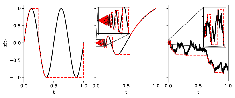
Figure 9. Illustration of a rough path $z$ (black line) and $\operatorname{orm}[z]$ (red dashed line). Left plot: $z(t)=\sin(4\pi t)$. Middle plot: $z(t)={\mathbf{1}_{t>0}}t\sin(\pi/(2t))$. Right plot: $z$ is a realization of a standard Wiener process.

It remains to verify that the orm functions are càdlàg.

Lemma 4.6.

For all $z\in C_{0}([0,T])$, $\operatorname{orm}[z]\in\mathcal{D}([0,T])$.

Proof.

Note first that if $t\in\bar{A}^{+}[z]([0,T])\cap\bar{A}^{-}[z]([0,T])$, then by (4.16),

$$z(t)=M^{+}[z](t)=M^{-}[z](t)\implies\text{$z(s)=0$ for all $s\in[0,t]$.}$$

By (4.16) and Definition 4.5, we have for all $t\in[0,T)$,

$$\begin{split}\operatorname{orm}[z](t)&=M^{+}[z](t){\mathbf{1}_{\bar{A}^{+}[z](t)>\bar{A}^{-}[z](t)}}+M^{-}[z](t){\mathbf{1}_{\bar{A}^{-}[z](t)>\bar{A}^{+}[z](t)}}\\ &=\begin{cases}M^{+}[z](t)=z(\bar{A}^{+}[z](t))&\text{if}\quad\bar{A}^{+}[z](t)\geq\bar{A}^{-}[z](t)\\ M^{-}[z](t)=z(\bar{A}^{-}[z](t))&\text{if}\quad\bar{A}^{-}[z](t)>\bar{A}^{+}[z](t),\end{cases}\end{split}$$

and $\operatorname{orm}[z](T)=z(T)$. Hence,

(4.24) $$\operatorname{orm}[z](t)=\begin{cases}z(\max(\bar{A}^{+}[z],\bar{A}^{-}[z])(t))&\text{if }t\in[0,T)\\ z(T)&\text{if }t=T,\end{cases}$$

and, since $z\in C_{0}([0,T])$ and

$$g(t)={\mathbf{1}_{t<T}}\max(\bar{A}^{+}[z],\bar{A}^{-}[z])(t)+{\mathbf{1}_{t=T}}T$$

is càdlàg whenever $\bar{A}^{+}[z],\bar{A}^{-}[z]\in\mathcal{D}([0,T])$, it follows that also $\operatorname{orm}[z]=z\circ g$ belongs to $\mathcal{D}([0,T])$.

∎

Theorem 4.7.

Assume that $f\in C^{2}(\mathbb{R})$ is strictly convex, $u_{0}\in(L^{1}\cap BV)(\mathbb{R})$, and $z\in C_{0}([0,T])$. For some $m\geq 2$, let $\{\tau_{k}\}_{k=0}^{m}$ be a set of points satisfying

$$0=\tau_{0}<\tau_{1}<\ldots<\tau_{m}=T,$$

$z^{m}=\mathcal{I}^{m}[z]$, and let

$$0=\tau_{j(0)}<\tau_{j(1)}<\ldots<\tau_{j(\bar{m})}=T$$

be the associated interpolation points of $\overline{\operatorname{orm}}[z](\cdot;\{\tau_{j(k)}\}_{k=0}^{\bar{m}})$, cf. Definition 4.3. Then

(4.25) $$v(T;\operatorname{orm}[z^{m}],\{\tau_{j(k)}\}_{k=0}^{\bar{m}})=v(T;\operatorname{orm}[z^{m}],\{\tau_{k}\}_{k=0}^{m})=u^{m}(T).$$

Proof.

Set $y^{m}=\overline{\operatorname{orm}}_{m}[z]$ and $\hat{y}^{m}=\operatorname{orm}[z^{m}]$. By (4.19), (4.24) and (4.15), it holds for all $k\in\{0,1,\ldots,\bar{m}-1\}$ that

(4.26) $$\begin{split}\hat{y}^{m}(\tau_{j(k)})&=z^{m}\left(\max(\bar{A}^{+}[z^{m}],\bar{A}^{-}[z^{m}])(\tau_{j(k)})\right)=z^{m}(\tau_{j(k)})=y^{m}(\tau_{j(k)}),\end{split}$$

and

$$\hat{y}^{m}(\tau_{j(\bar{m})})=z^{m}(T)=y^{m}(\tau_{j(\bar{m})}).$$

By Theorem 4.5,

(4.27) $$\bar{}\mathcal{S}(\Delta y_{\tau_{j(\bar{m})-1}}^{m})\cdots\bar{}\mathcal{S}(\Delta y_{\tau_{j(0)}}^{m})u_{0}\\ =\bar{}\mathcal{S}(y^{m}(\tau_{j(\bar{m})})-y^{m}(\tau_{j(\bar{m}-1)}))\cdots\bar{}\mathcal{S}(y^{m}(\tau_{j(1)})-y^{m}(\tau_{j(0)}))u_{0}=u^{m}(T);$$

so to verify (4.25), it suffices to show that for all $k\in\{0,1,\ldots,\bar{m}-1\}$,

(4.28) $$\bar{}\mathcal{S}(\Delta\hat{y}_{j(k+1)-1}^{m})\ldots\bar{}\mathcal{S}(\Delta\hat{y}_{j(k)}^{m})u^{m}(\tau_{j(k)})\\ =\bar{}\mathcal{S}(y^{m}(\tau_{j(k+1)})-y^{m}(\tau_{j(k)}))u^{m}(\tau_{j(k)}).$$

For $k\in\{0,1,\ldots,\bar{m}-1\}$ such that $j(k+1)-j(k)=1$, (4.28) holds by (4.26).

Assume next that $k\in\{0,1,\ldots,\bar{m}-1\}$ is such that $j(k+1)-j(k)\geq 2$. If $k=\bar{m}-1$ and $\tau_{j(k+1)}=T\notin A^{\pm}[z^{m}]$, then

$$z^{m}([\tau_{j(k)},T])\subset[M^{-}[z^{m}](\tau_{j(k)}),M^{+}[z^{m}](\tau_{j(k)})].$$

It follows that $M^{+}[z^{m}],M^{-}[z^{m}],\bar{A}^{+}[z^{m}]$ and $\bar{A}^{-}[z^{m}]$ are constant over $[\tau_{j(\bar{m}-1)},T)$, which implies that $\hat{y}^{m}$ is constant over $[\tau_{j(k)},T)$. Hence $\hat{y}^{m}(\tau_{j(\bar{m})-1})=\hat{y}^{m}(\tau_{j(\bar{m}-1)})$,

(4.29) $$\Delta\hat{y}_{j(\bar{m})-\ell}^{m}=0\quad\forall\ell\in\{2,\ldots,j(\bar{m})-j(\bar{m}-1)\},$$

and since $\bar{}\mathcal{S}(0)=I$,

$$\bar{}\mathcal{S}(\Delta\hat{y}_{j(\bar{m})-1}^{m})\cdots\bar{}\mathcal{S}(\Delta\hat{y}_{j(\bar{m}-1)}^{m})u^{m}(\tau_{j(\bar{m}-1)})$$

$$\qquad=\bar{}\mathcal{S}(\Delta\hat{y}_{j(\bar{m})-1}^{m})u^{m}(\tau_{j(\bar{m}-1)})$$

$$\qquad=\bar{}\mathcal{S}(y^{m}(\tau_{j(\bar{m})})-y^{m}(\tau_{j(\bar{m}-1)}))u^{m}(\tau_{j(\bar{m}-1)}).$$

Otherwise, if $k\in\{0,1,\ldots,\bar{m}-1\}$ is such that $j(k+1)-j(k)\geq 2$ and $\tau_{j(k+1)}\in A^{\pm}[z]$, then we recall from the proof of Theorem 4.5 that there exists a unique $\tau\in(\tau_{j(k+1)-1},\tau_{j(k+1)}]$ such that

$$z^{m}([\tau_{j(k)},\tau])\subset[M^{-}[z^{m}](\tau_{j(k)}),M^{+}[z^{m}](\tau_{j(k)})],\quad\tau\in\{\bar{A}^{+}(\tau),\bar{A}^{-}(\tau)\}.$$

This implies that $\hat{y}^{m}(\tau)=z^{m}(\tau)$, cf. (4.24), and that $M^{+}[z^{m}],M^{-}[z^{m}],\bar{A}^{+}[z^{m}]$, $\bar{A}^{-}[z^{m}]$ are constant over the interval $[\tau_{j(k)},\tau)$. Consequently, $\hat{y}^{m}$ is constant over $[\tau_{j(k)},\tau)$, and since $\tau_{j(k+1)-1}<\tau$, $\hat{y}^{m}(\tau_{j(k+1)-1})=\hat{y}^{m}(\tau_{j(k)})$ and

(4.30) $$\Delta\hat{y}_{j(k+1)-\ell}^{m}=0\quad\forall\ell\in\{2,\ldots,j(k+1)-j(k)\}.$$

Hence,

$$\begin{split}\bar{}\mathcal{S}(\Delta\hat{y}_{j(k+1)-1}^{m})\cdots\bar{}\mathcal{S}(\Delta\hat{y}_{j(k)}^{m})u^{m}(\tau_{j(k)})&=\bar{}\mathcal{S}(\Delta\hat{y}_{j(k+1)-1}^{m})u^{m}(\tau_{j(k)})\\ &=\bar{}\mathcal{S}(y^{m}(\tau_{j(k+1)})-y^{m}(\tau_{j(k)}))u^{m}(\tau_{j(k)}).\end{split}$$

∎

A direct consequence of the preceding proof is that the total variation of $\operatorname{orm}[\mathcal{I}^{m}[z]]$ equals the total variation of $\overline{\operatorname{orm}}_{m}[z]$.

Lemma 4.8.

For any $z\in C_{0}([0,T])$ and points $0=\tau_{0}<\tau_{1}<\ldots<\tau_{m}=T$, $m\geq 2$, it holds that

$${\left|\operatorname{orm}[\mathcal{I}[z](\cdot;\{\tau_{k}\}_{k=0}^{m})]\right|}_{\mathrm{BV}([0,T])}={\left|\overline{\operatorname{orm}}[z](\cdot;\{\tau_{k}\}_{k=0}^{m})\right|}_{\mathrm{BV}([0,T])}.$$

Proof.

Recall that $y^{m}=\overline{\operatorname{orm}}_{m}[z]\in I_{0}([0,T];\{\tau_{k}\}_{k=0}^{m})$ is piecewise linear, with interpolation points $0=\tau_{j(0)}<\tau_{j(1)}<\ldots<\tau_{j(\bar{m})}=T$. Hence, $y^{m}$ is monotone over each interval $[\tau_{j(k)},\tau_{j(k+1)}]$. Since $z^{m}=\mathcal{I}^{m}[z]$ is linear over every interval $[\tau_{k},\tau_{k+1}]$, it follows by Definition 4.5 that $\hat{y}^{m}=\operatorname{orm}[z^{m}]$ is monotone over every interval $[\tau_{k},\tau_{k+1}]$, and by the proof of Theorem 4.7, for every interval $[\tau_{j(k)},\tau_{j(k+1)}]$ with $j(k+1)-j(k)\geq 2$, it holds that $\hat{y}^{m}$ is constant over $[\tau_{j(k)},\tau_{j(k+1)-1}]$. Consequently, $\hat{y}^{m}$ is monotone over each interval $[\tau_{j(k)},\tau_{j(k+1)}]$, whereby

$${\left|\hat{y}^{m}\right|}_{\mathrm{BV}([\tau_{j(k)},\tau_{j(k+1)}])}={\left|\hat{y}^{m}(\tau_{j(k+1)})-\hat{y}^{m}(\tau_{j(k)})\right|}\quad\forall k\in\{0,1,\ldots,\bar{m}-1\}.$$

By (4.26),

$$\begin{split}{\left|\hat{y}^{m}\right|}_{\mathrm{BV}([0,T])}&=\sum_{k=0}^{\bar{m}-1}{\left|\hat{y}^{m}\right|}_{\mathrm{BV}([\tau_{j(k)},\tau_{j(k+1)}])}\\ &=\sum_{k=0}^{\bar{m}-1}{\left|\hat{y}^{m}(\tau_{j(k+1)})-\hat{y}^{m}(\tau_{j(k)})\right|}\\ &=\sum_{k=0}^{\bar{m}-1}{\left|y^{m}(\tau_{j(k+1)})-y^{m}(\tau_{j(k)})\right|}={\left|y^{m}\right|}_{\mathrm{BV}([0,T])}.\end{split}$$

∎

Definition 4.6.

For any mesh $\{\tau_{k}\}_{k=0}^{m}$ such that

$$0=\tau_{0}<\tau_{1}<\cdots<\tau_{m}=T,$$

and $g\in\mathcal{D}([0,T])$ we define the total variation of $g$ restricted to $\{\tau_{k}\}_{k=0}^{m}$ by

$$TV(g;\{\tau_{k}\}_{k=0}^{m})\mathrel{\vbox{\hbox{\scriptsize.}\hbox{\scriptsize.}}}=\sum_{k=0}^{m-1}|g(\tau_{k+1})-g(\tau_{k})|.$$

The next lemma shows that the approximation $v(T;\operatorname{orm}[z],\{\tau_{j}\}_{j=0}^{m})$ converges to a limit in $L^{1}(\mathbb{R})$ as $m\to\infty$, and it provides an upper bound for the approximation error. The upper bound depends on $\operatorname{orm}[z]$, the mesh $\{\tau_{k}\}_{k=0}^{m}$, $|u_{0}|_{\mathrm{BV}((\mathbb{R}))}$ and $\|f^{\prime}\|_{\infty}$, hence it differs from the stability result (2.3).

Lemma 4.9.

Let $\{\{\tau^{m}_{k}\}_{k=0}^{\ell_{m}}\}_{m=0}^{\infty}$ denote a sequence of nested meshes fulfilling $\ell_{0}\geq 2$, and for all $m\geq 0$,

$$0=\tau^{m}_{0}<\tau^{m}_{1}<\cdots<\tau^{m}_{\ell_{m}}=T,\quad\text{with}\quad\ell_{m}<\ell_{m+1}\leq 2\ell_{m},$$

and the nested mesh property

$$\{\tau^{m}_{k}\}_{k=0}^{\ell_{m}}\subset\{\tau^{m+1}_{k}\}_{k=0}^{\ell_{m+1}}$$

with a strictly increasing mapping $j^{m}:\{0,1,\ldots,\ell_{m}\}\to\{0,1,\ldots,\ell_{m+1}\}$ such that

$$\tau_{j^{m}(k)}^{m+1}=\tau^{m}_{k},\quad\forall k\in\{0,1,\ldots,\ell_{m}\},$$

and

$$1\leq j^{m}(k+1)-j^{m}(k)\leq 2,\quad\forall k\in\{0,1,\ldots,\ell_{m}-1\}.$$

Assume $f\in C^{2}(\mathbb{R})$ is strictly convex, $u_{0}\in(L^{1}\cap BV)(\mathbb{R})$, $z\in C_{0}([0,T])$. Then, for any $\widehat{m},\overline{m}\in\mathbb{N}\cup\{0\}$ with $\widehat{m}\geq\overline{m}$,

(4.31) $$\begin{split}&{\left\|v(T;\operatorname{orm}[z],\{\tau_{k}^{\widehat{m}}\}_{k=0}^{\ell_{\widehat{m}}})-v(T;\operatorname{orm}[z],\{\tau_{k}^{\overline{m}}\}_{k=0}^{\ell_{\overline{m}}})\right\|}_{L^{1}(\mathbb{R})}\\ &\qquad\leq 2\|f^{\prime}\|_{\infty}|u_{0}|_{\mathrm{BV}(\mathbb{R})}\left(TV(\operatorname{orm}[z];\{\tau_{k}^{\widehat{m}}\}_{k=0}^{\ell_{\widehat{m}}})-TV(\operatorname{orm}[z];\{\tau_{k}^{\overline{m}}\}_{k=0}^{\ell_{\overline{m}}})\right).\end{split}$$

Moreover, if

$${\left|\operatorname{orm}[z]\right|}_{\mathrm{BV}([0,T])}<\infty,$$

and

(4.32) $$\lim_{m\to\infty}\left({\left|\operatorname{orm}[z]\right|}_{\mathrm{BV}([0,T])}-TV(\operatorname{orm}[z];\{\tau_{k}^{m}\}_{k=0}^{\ell_{m}})\right)=0,$$

then

$$v_{\operatorname{orm}}(T)\mathrel{\vbox{\hbox{\scriptsize.}\hbox{\scriptsize.}}}=\lim_{m\to\infty}v(T;\operatorname{orm}[z],\{\tau_{k}^{m}\}_{k=0}^{\ell_{m}})\in L^{1}(\mathbb{R})$$

and

(4.33) $$\begin{split}&\|v_{\operatorname{orm}}(T)-v(T;\operatorname{orm}[z],\{\tau_{k}^{m}\}_{k=0}^{\ell_{m}})\|_{1}\\ &\qquad\leq 2\|f^{\prime}\|_{\infty}|u_{0}|_{\mathrm{BV}(\mathbb{R})}\left({\left|\operatorname{orm}[z]\right|}_{\mathrm{BV}([0,T])}-TV(\operatorname{orm}[z];\{\tau_{k}^{m}\}_{k=0}^{\ell_{m}})\right).\end{split}$$

Proof.

For a fixed $m\geq 0$, set $y=\operatorname{orm}[z]$, $\Delta y^{m}_{k}=y(\tau^{m}_{k+1})-y(\tau^{m}_{k})$, and introduce the shorthand

$$v^{m}(\tau_{k}^{m})=v(\tau_{k}^{m};y,\{\tau_{k}^{m+1}\}_{k=0}^{\ell_{m}}),\quad\text{for all }k\in\{0,1,\ldots,\ell_{m}\}.$$

We have that

(4.34) $$\begin{split}&\|v^{m+1}(T)-v^{m}(T)\|_{L^{1}(\mathbb{R})}\\ &\quad={\left\|\bar{}\mathcal{S}(\Delta y^{m+1}_{\ell_{m+1}-1})\cdots\bar{}\mathcal{S}(\Delta y^{m+1}_{0})u_{0}-\bar{}\mathcal{S}(\Delta y^{m}_{\ell_{m}-1})\cdots\bar{}\mathcal{S}(\Delta y^{m}_{0})u_{0}\right\|}_{L^{1}(\mathbb{R})}\\ &\quad\leq\sum_{k\in J^{m}_{2}}\|\Delta\bar{}\mathcal{S}_{k}u_{0}\|_{L^{1}(\mathbb{R})},\end{split}$$

where $J^{m}_{2}=\{k\in\{0,1,\ldots,\ell_{m}-1\}\mid j^{m}(k+1)-j^{m}(k)=2\}$ and

$$\begin{split}&\Delta\bar{}\mathcal{S}_{k}u_{0}\mathrel{\vbox{\hbox{\scriptsize.}\hbox{\scriptsize.}}}=\\ &\begin{cases}0&\text{if }k\notin J^{m}_{2},\\ \!\begin{aligned} &\bar{}\mathcal{S}(\Delta y^{m+1}_{\ell_{m+1}-1})\cdots\bar{}\mathcal{S}(\Delta y^{m+1}_{j^{m}(k+1)})\\ &\left(\bar{}\mathcal{S}(\Delta y^{m+1}_{j^{m}(k)+1})\bar{}\mathcal{S}(\Delta y^{m+1}_{j^{m}(k)})-\bar{}\mathcal{S}(\Delta y^{m}_{k})\right)v^{m}(\tau^{m}_{k})\end{aligned}&\text{if }k\in J^{m}_{2}\cap[0,\ell_{m}-2],\\ \left(\bar{}\mathcal{S}(\Delta y^{m+1}_{\ell_{m+1}-1})\bar{}\mathcal{S}(\Delta y^{m+1}_{\ell_{m+1}-2})-\bar{}\mathcal{S}(\Delta y^{m}_{\ell_{m}-1})\right)v^{m}(\tau^{m}_{\ell_{m}-1})&\text{if }k\in J^{m}_{2}\cap\{\ell_{m}-1\}.\end{cases}\end{split}$$

Assume that $k\in J^{m}_{2}$. Using (4.8), we obtain the following bound

$$\begin{split}\|\Delta\bar{}\mathcal{S}_{k}u_{0}\|_{L^{1}(\mathbb{R})}&\leq{\left\|\left(\bar{}\mathcal{S}(\Delta y^{m+1}_{j^{m}(k)+1})\bar{}\mathcal{S}(\Delta y^{m+1}_{j^{m}(k)})-\bar{}\mathcal{S}(\Delta y^{m}_{k})\right)v^{m}(\tau^{m}_{k})\right\|}_{L^{1}(\mathbb{R})}.\end{split}$$

We recall from (4.4) that $\bar{}\mathcal{S}(\Delta y^{m+1}_{j^{m}(k)+1})\bar{}\mathcal{S}(\Delta y^{m+1}_{j^{m}(k)})v^{m}(\tau^{m}_{k})$ is recursively defined by being the solution at time $t=|\Delta y^{m+1}_{j^{m}(k)+1}|$ of

$$\partial_{t}\tilde{u}+\operatorname*{sign}\left(\Delta y^{m+1}_{j^{m}(k)+1}\right)\partial_{x}f(\tilde{u})=0,\quad t>0,\quad\tilde{u}(0)=\bar{}\mathcal{S}(\Delta y^{m+1}_{j^{m}(k)})v^{m}(\tau^{m}_{k}).$$

If $\Delta y^{m+1}_{j^{m}(k)+1}\Delta y^{m+1}_{j^{m}(k)}\geq 0$, then

(4.35) $$\begin{split}\bar{}\mathcal{S}(\Delta y^{m+1}_{j^{m}(k)+1})\bar{}\mathcal{S}(\Delta y^{m+1}_{j^{m}(k)})v^{m}(\tau^{m}_{k})&=\bar{}\mathcal{S}(\Delta y^{m+1}_{j^{m}(k)+1}+\Delta y^{m+1}_{j^{m}(k)})v^{m}(\tau^{m}_{k})\\ &=\bar{}\mathcal{S}(\Delta y^{m}_{k})v^{m}(\tau^{m}_{k}).\end{split}$$

This yields

(4.36) $$\|\Delta\bar{}\mathcal{S}_{k}u_{0}\|_{L^{1}(\mathbb{R})}=0,\quad\forall k\in\{\bar{k}\in J^{m}_{2}\mid\Delta y^{m+1}_{j^{m}(\bar{k})+1}\Delta y^{m+1}_{j^{m}(\bar{k})}\geq 0\}.$$

Consider next the case $\Delta y^{m+1}_{j^{m}(k)+1}\Delta y^{m+1}_{j^{m}(k)}<0$. In view of Definition 4.5, $y(\tau^{m}_{k+1})\in\{M^{+}[z](\tau^{m}_{k+1}),M^{-}[z](\tau^{m}_{k+1})\}$. If $y(\tau^{m}_{k+1})=M^{+}[z](\tau^{m}_{k+1})$, then

$$y(\tau^{m+1}_{j^{m}(k)+1)})\leq y(\tau^{m}_{k+1})=y(\tau^{m+1}_{j^{m}(k+1))}),$$

while if $y(\tau^{m}_{k+1})=M^{-}[z](\tau^{m}_{k+1})$, then

$$y(\tau^{m+1}_{j^{m}(k)+1})\geq y(\tau^{m}_{k+1})=y(\tau^{m+1}_{j^{m}(k+1))}).$$

We conclude that regardless of whether $y(\tau^{m}_{k+1})=M^{+}[z](\tau^{m}_{k+1})$ or $y(\tau^{m}_{k+1})=M^{-}[z](\tau^{m}_{k+1})$, it holds that

(4.37) $$\Delta y^{m+1}_{j^{m}(k)+1}\Delta y^{m}_{k}=\left(y(\tau^{m}_{k+1})-y(\tau^{m+1}_{j^{m}(k)+1})\right)\left(y(\tau^{m}_{k+1})-y(\tau^{m}_{k})\right)\geq 0.$$

And since

$$\operatorname*{sign}\left(\Delta y^{m}_{k}\left(-\Delta y^{m+1}_{j^{m}(k)}\right)\right)=\operatorname*{sign}\left(\Delta y^{m}_{k}\Delta y^{m+1}_{j^{m}(k+1)}\right)\geq 0,$$

we also have that

$$\Delta y^{m}_{k}\left(-\Delta y^{m+1}_{j^{m}(k)}\right)\geq 0.$$

Using the relationship

$$\Delta y^{m+1}_{j^{m}(k)+1}=\Delta y^{m}_{k}-\Delta y^{m+1}_{j^{m}(k)}$$

we obtain

$$\begin{split}&\bar{}\mathcal{S}(\Delta y^{m}_{k})\bar{}\mathcal{S}\left(-\Delta y^{m+1}_{j^{m}(k)}\right)\bar{}\mathcal{S}\left(\Delta y^{m+1}_{j^{m}(k)}\right)v^{m}(\tau^{m}_{k})\\ &\qquad\qquad=\bar{}\mathcal{S}\left(\Delta y^{m}_{k}-\Delta y^{m+1}_{j^{m}(k)}\right)\bar{}\mathcal{S}\left(\Delta y^{m+1}_{j^{m}(k)}\right)v^{m}(\tau^{m}_{k})\\ &\qquad\qquad=\bar{}\mathcal{S}\left(\Delta y^{m+1}_{j^{m}(k)+1}\right)\bar{}\mathcal{S}\left(\Delta y^{m+1}_{j^{m}(k)}\right)v^{m}(\tau^{m}_{k}).\end{split}$$

By (4.8), (4.9) and (4.10), we derive the following bound for all $k\in J^{m}_{2}$ such that $\Delta y^{m+1}_{j^{m}(k)+1}\Delta y^{m+1}_{j^{m}(k)}<0$,

(4.38) $$\begin{split}\|\Delta\bar{}\mathcal{S}_{k}u_{0}\|_{L^{1}(\mathbb{R})}&\leq{\left\|\bar{}\mathcal{S}(\Delta y^{m}_{k})\left(\bar{}\mathcal{S}(-\Delta y^{m+1}_{j^{m}(k)})\bar{}\mathcal{S}(\Delta y^{m+1}_{j^{m}(k)})-I\right)v^{m}(\tau^{m}_{k})\right\|}_{L^{1}(\mathbb{R})}\\ &\leq{\left\|\left(\bar{}\mathcal{S}(-\Delta y^{m+1}_{j^{m}(k)})\bar{}\mathcal{S}(\Delta y^{m+1}_{j^{m}(k)})-I\right)v^{m}(\tau^{m}_{k})\right\|}_{L^{1}(\mathbb{R})}\\ &\leq{\left\|\left(\bar{}\mathcal{S}(-\Delta y^{m+1}_{j^{m}(k)})-I\right)\bar{}\mathcal{S}(\Delta y^{m+1}_{j^{m}(k)})v^{m}(\tau^{m}_{k})\right\|}_{L^{1}(\mathbb{R})}\\ &\qquad+{\left\|\left(\bar{}\mathcal{S}(\Delta y^{m+1}_{j^{m}(k)})-I\right)v^{m}(\tau^{m}_{k})\right\|}_{L^{1}(\mathbb{R})}\\ &\leq 2\|f^{\prime}\|_{\infty}|u_{0}|_{\mathrm{BV}(\mathbb{R})}|\Delta y^{m+1}_{j^{m}(k)}|.\end{split}$$

By (4.34), (4.36) and (4.38),

(4.39) $$\begin{split}\|v^{m+1}(T)-v^{m}(T)\|_{L^{1}(\mathbb{R})}&\leq\sum_{k\in J^{m}_{2}}2\|f^{\prime}\|_{\infty}|u_{0}|_{\mathrm{BV}(\mathbb{R})}|\Delta y^{m+1}_{j^{m}(k)}|\\ &\leq 2\|f^{\prime}\|_{\infty}|u_{0}|_{\mathrm{BV}(\mathbb{R})}\Bigl{(}\sum_{k=0}^{\ell_{m+1}}|\Delta y^{m+1}_{k}|-\sum_{k=0}^{\ell_{m}}|\Delta y^{m}_{k}|\Bigr{)}.\end{split}$$

For $m_{2}>m_{1}$ we get

$${\left\|v^{m_{2}}(T)-v^{m_{1}}(T)\right\|}_{L^{1}(\mathbb{R})} \leq\sum_{m=m_{1}}^{m_{2}-1}{\left\|v^{m+1}(T)-v^{m}(T)\right\|}_{L^{1}(\mathbb{R})}$$

$$\leq 2\|f^{\prime}\|_{\infty}|u_{0}|_{\mathrm{BV}(\mathbb{R})}\sum_{m=m_{1}}^{m_{2}-1}\Bigl{(}\sum_{k=0}^{\ell_{m+1}}|\Delta y^{m+1}_{k}|-\sum_{k=0}^{\ell_{m}}|\Delta y^{m}_{k}|\Bigr{)}$$

$$=2\|f^{\prime}\|_{\infty}|u_{0}|_{\mathrm{BV}(\mathbb{R})}\Bigr{(}\sum_{k=0}^{\ell_{m_{2}+1}}|\Delta y^{m_{2}+1}_{k}|-\sum_{k=0}^{\ell_{m_{1}}}|\Delta y^{m_{1}}_{k}|\Bigr{)}$$

By assumption (4.32), both sums on the right converge to ${\left|\operatorname{orm}[z]\right|}_{\mathrm{BV}([0,T])}$, thus $\{v^{m}(T)\}_{m}\subset L^{1}(\mathbb{R})$ is a Cauchy sequence, and,

$$\lim_{m\to\infty}v^{m}(T)=v_{\operatorname{orm}}(T)\in L^{1}(\mathbb{R}).$$

Moreover, by (4.39), (4.32) and a telescoping sum argument we obtain

$$\|v_{\operatorname{orm}}(T)-v^{m}(T)\|_{L^{1}(\mathbb{R})}\leq 2\|f^{\prime}\|_{\infty}|u_{0}|_{\mathrm{BV}(\mathbb{R})}\Bigl{(}{\left|\operatorname{orm}[z]\right|}_{\mathrm{BV}([0,T])}-\sum_{k=0}^{\ell_{m}}|\Delta y^{m}_{k}|\Bigr{)}.$$

Inequality (4.31) can be proved using a similar telescoping sum argument. ∎

It remains to verify that $v_{\operatorname{orm}}(T)$, under some assumptions, is equal to the unique pathwise entropy solution of (1.5) at time $t=T$.

Theorem 4.10.

Let $u$ denote the unique pathwise entropy solution of (1.5) with initial data $u_{0}\in(L^{1}\cap BV)(\mathbb{R})$, strictly convex flux $f\in C^{2}(\mathbb{R})$ and driving path $z\in C_{0}([0,T])$. Assume that ${\left|\operatorname{orm}[z]\right|}_{\mathrm{BV}(\mathbb{R})}<\infty$ and for some $m\geq 2$, let $\{\tau_{j=0}\}_{j=0}^{m}$ denote a mesh satisfying

$$0=\tau_{0}<\tau_{1}<\ldots<\tau_{m}=T.$$

Then

$$\begin{split}&\|u(T)-v(T;\operatorname{orm}[z],\{\tau_{k}\}_{k=0}^{m})\|_{L^{1}(\mathbb{R})}\\ &\qquad\qquad\leq 2\|f^{\prime}\|_{\infty}|u_{0}|_{\mathrm{BV}(\mathbb{R})}\left({\left|\operatorname{orm}[z]\right|}_{\mathrm{BV}([0,T])}-TV(\operatorname{orm}[z];\{\tau_{k}\}_{k=0}^{m})\right).\end{split}$$

Proof.

Since ${\left|\operatorname{orm}[z]\right|}_{BV([0,T])}<\infty$, there is a sequence of meshes $\{\{\tau^{r}_{k}\}_{k=1}^{\ell_{r}}\}_{r=0}^{\infty}$ such that

$$\lim_{r\to\infty}TV(\operatorname{orm}[z];\{\tau_{k}^{r}\}_{k=0}^{\ell_{r}})={\left|\operatorname{orm}[z]\right|}_{\mathrm{BV}([0,T])}.$$

If necessary, we can add meshpoints to get nested meshes $\{\{\hat{\tau}_{k}^{r}\}_{k=0}^{\hat{\ell}_{r}}\}_{r=0}^{\infty}$ fulfilling that $\{\hat{\tau}_{k}^{0}\}_{k=0}^{\hat{\ell}_{0}}=\{\tau_{k}\}_{k=0}^{m}$, $\hat{\ell}_{r}<\hat{\ell}_{r+1}$ for all $r\geq 0$,

$$\lim_{r\to\infty}\max_{k\in\{0,1,\ldots,\ell_{m}-1\}}\hat{\tau}^{r}_{k+1}-\hat{\tau}_{k}^{r}=0,$$

and

$$\lim_{r\to\infty}TV(\operatorname{orm}[z];\{\hat{\tau}_{k}^{r}\}_{k=0}^{\hat{\ell}_{r}})={\left|\operatorname{orm}[z]\right|}_{BV([0,T])}.$$

Let

(4.40) $$A^{\pm}_{r}[z]\mathrel{\vbox{\hbox{\scriptsize.}\hbox{\scriptsize.}}}=\bar{A}^{+}[z](\{\hat{\tau}_{k}^{r}\}_{k=0}^{\hat{\ell}_{r}})\cup\bar{A}^{-}[z](\{\hat{\tau}_{k}^{r}\}_{k=0}^{\hat{\ell}_{r}}),\quad r\geq 0.$$

As $A^{\pm}_{r}[z]\subset A^{\pm}_{r+1}[z]$ for all $r\geq 0$, we may construct a new sequence of nested meshes $\{\{\tau_{k}^{r}\}_{k=0}^{\ell_{r}}\}_{r=0}^{\infty}$ defined by

(4.41) $$\{\tau_{k}^{r}\}_{k=0}^{\ell_{r}}=\begin{cases}\{\hat{\tau}_{k}^{0}\}_{k=0}^{\hat{\ell}_{0}}=\{\tau_{k}\}_{k=0}^{m},&\text{if }r=0,\\ \{\hat{\tau}_{k}^{r-1}\}_{k=0}^{\hat{\ell}_{r-1}}\cup A^{\pm}_{r-1}[z],&\text{if }r\geq 1.\end{cases}$$

Since $\{\tau_{k}^{r}\}_{k=0}^{\ell_{r}}\supset\{\hat{\tau}_{k}^{r}\}_{k=0}^{\hat{\ell}_{r}}$ for all $r\geq 0$, it also holds that

(4.42) $$\lim_{r\to\infty}\max_{k\in\{0,1,\ldots,\ell_{r}-1\}}\tau^{r}_{k+1}-\tau_{k}^{r}=0,$$

and

$$\lim_{r\to\infty}TV(\operatorname{orm}[z];\{\tau_{k}^{r}\}_{k=0}^{\ell_{r}})={\left|\operatorname{orm}[z]\right|}_{BV([0,T])}.$$

For any $r\geq 1$, we have that

(4.43) $$\begin{split}&\|v(T;\operatorname{orm}[z],\{\tau_{k}\}_{k=0}^{m})-u(T)\|_{L^{1}(\mathbb{R})}\\ &\qquad\leq\|v(T;\operatorname{orm}[z],\{\tau_{k}\}_{k=0}^{m})-v(T;\operatorname{orm}[z],\{\tau_{k}^{r}\}_{k=0}^{\ell_{r}})\|_{L^{1}(\mathbb{R})}\\ &\qquad\qquad+\|v(T;\operatorname{orm}[z],\{\tau_{k}^{r}\}_{k=0}^{\ell_{r}})-u(T)\|_{L^{1}(\mathbb{R})}\\ &\qquad=\mathrel{\vbox{\hbox{\scriptsize.}\hbox{\scriptsize.}}}\mathrm{I}_{r}+\mathrm{II}_{r}.\end{split}$$

Lemma 4.9 implies that for any pair of nested meshes $\{\tau_{k}\}_{k=0}^{m}\subset\{\tau_{k}^{r}\}_{k=0}^{\ell_{r}}$,

(4.44) $$\begin{split}\mathrm{I}_{r}&\leq 2\|f^{\prime}\|_{\infty}|u_{0}|_{\mathrm{BV}(\mathbb{R})}\left(TV(\operatorname{orm}[z];\{\tau_{k}^{r}\}_{k=0}^{\ell_{r}})-TV(\operatorname{orm}[z];\{\tau_{k}\}_{k=0}^{m})\right)\\ &\leq 2\|f^{\prime}\|_{\infty}|u_{0}|_{\mathrm{BV}(\mathbb{R})}\left({\left|\operatorname{orm}[z]\right|}_{BV([0,T])}-TV(\operatorname{orm}[z];\{\tau_{k}\}_{k=0}^{m})\right).\end{split}$$

To bound $\mathrm{II}_{r}$, note first that by (4.24),

$$\operatorname{orm}[z](\tau_{k}^{r})=\begin{cases}z(\max(A^{+}[z],A^{-}[z])(\tau_{k}^{r}))&\text{if}\quad k\in\{0,1,\ldots,\ell_{r}-1\},\\ z(T)=z(\tau_{\ell_{r}}^{r})&\text{if}\quad k=\ell_{r}.\end{cases}$$

Recalling that $\hat{}\mathcal{S}(0)=I$ and that $\max(\bar{A}^{+}[z],\bar{A}^{-}[z])(\cdot)$ is a monotonically increasing function,

(4.45) $$\begin{split}&v(T;\operatorname{orm}[z],\{\tau_{k}^{r}\}_{k=0}^{\ell_{r}})\\ &=\bar{}\mathcal{S}(\operatorname{orm}[z](\tau^{r}_{\ell_{r}})-\operatorname{orm}[z](\tau^{r}_{\ell_{r}-1}))\cdots\bar{}\mathcal{S}(\operatorname{orm}[z](\tau^{r}_{1})-\operatorname{orm}[z](\tau^{r}_{0}))u_{0}\\ &=v(T;z,\max(A^{+}[z],A^{-}[z])(\{\tau_{k}^{r}\}_{k=0}^{\ell_{r}})\cup\{T\}).\end{split}$$

By (4.17),

$$\max\left\{\bar{A}^{+}[z],\bar{A}^{-}[z]\right\}(A^{\pm}_{r}[z])=A^{\pm}_{r}[z],$$

and (4.41) implies that

$$\begin{split}&\max(\bar{A}^{+}[z],\bar{A}^{-}[z])(\{\tau_{k}^{{r}}\}_{k=0}^{\ell_{r}})=\max(\bar{A}^{+}[z],\bar{A}^{-}[z])(A^{\pm}_{r}[z]\cup\{\hat{\tau}_{k}^{{r}}\}_{k=0}^{\hat{\ell}_{r}})\\ &\qquad\qquad\qquad=\max(\bar{A}^{+}[z],\bar{A}^{-}[z])(A^{\pm}_{r}[z])\,\cup\,\max(\bar{A}^{+}[z],\bar{A}^{-}[z])(\{\hat{\tau}_{k}^{r}\}_{k=0}^{\hat{\ell}_{r}})\\ &\qquad\qquad\qquad=A^{\pm}_{r}[z].\end{split}$$

Consequently,

$$\begin{split}v(T;z,\max(A^{+}[z],A^{-}[z])(\{\tau_{k}^{r}\}_{k=0}^{\ell_{r}})\cup\{T\})&=v(T;z,A^{\pm}_{r}[z]\cup\{T\})\\ &=v(T;\tilde{z}^{r},A^{\pm}_{r}[z]\cup\{T\}),\end{split}$$

where $\tilde{z}^{r}\mathrel{\vbox{\hbox{\scriptsize.}\hbox{\scriptsize.}}}=\mathcal{I}[z](\cdot;A^{\pm}_{r}[z]\cup\{T\})$. Introducing the function $z^{r}=\mathcal{I}[z](\cdot;\{\tau_{k}^{r}\}_{k=0}^{\ell_{r}})$, we may bound the second term as follows

(4.46) $$\begin{split}\mathrm{II}_{r}&\leq{\left\|u(T)-v(T;z^{r},\{\tau_{k}^{r}\}_{k=0}^{\ell_{r}})\right\|}_{1}+{\left\|v(T;z^{r},\{\tau_{k}^{r}\}_{k=0}^{\ell_{r}})-v(T;\tilde{z}^{r},A^{\pm}_{r}[z]\cup\{T\})\right\|}_{1}\\ &=\mathrel{\vbox{\hbox{\scriptsize.}\hbox{\scriptsize.}}}\mathrm{II}_{r,1}+\mathrm{II}_{r,2}.\end{split}$$

Theorem 2.1 and the property $z^{r}(T)=z(T)$ for all $r\geq 1$ imply that there exists a constant $C(\|u_{0}\|_{2},\|f^{\prime\prime}\|_{\infty})>0$ such that

$$\mathrm{II}_{r,1}\leq C\sqrt{\max_{s\in[0,T]}{\left|z-z^{r}\right|}(s)},\quad\forall r\geq 1.$$

Since $z$ is uniformly continuous on $[0,T]$, and it follows from (4.42) that

(4.47) $$\lim_{r\to\infty}\mathrm{II}_{r,1}=0.$$

The term $\mathrm{II}_{r,2}$ is bounded by verifying that

(4.48) $$v(T;z^{r},\{\tau_{k}^{r}\}_{k=0}^{\ell_{r}})=v(T;\tilde{z}^{r},A^{\pm}_{r}[z]\cup\{T\}),$$

which actually means that $\mathrm{II}_{r,2}=0$. Note first that since $A^{\pm}_{r}[z]\cup\{T\}\subset\{\tau_{k}^{r}\}_{k=0}^{\ell_{r}}$, we may introduce the monotonically increasing function $h:\{0,1,\ldots,\ell_{r}\}\to\{0,1,\ldots,\ell_{r}\}$ defined by

$$h(k)=\begin{cases}\{s\in\{0,1,\ldots,k\}\mid\tau_{s}^{r}=\max(\bar{A}^{+}[z],\bar{A}^{-}[z])(\tau^{r}_{k})\}&\text{if }k<\ell_{r},\\ \ell_{r}&\text{if }k=\ell_{r}.\end{cases}$$

and write $\{\tau_{h(k)}\}_{k=0}^{\ell_{r}}=A^{\pm}_{r}[z]\cup\{T\}$. Using this representation and that

$$\tilde{z}^{r}|_{A^{\pm}_{r}[z]\cup\{T\}}=z|_{A^{\pm}_{r}[z]\cup\{T\}}=z^{r}|_{A^{\pm}_{r}[z]\cup\{T\}},$$

we obtain

$$v(T;\tilde{z}^{r},\{\tau_{h(k)}\}_{k=0}^{\ell_{r}})=\bar{}\mathcal{S}\left(z^{r}(\tau_{h(\ell_{r})}^{r})-z^{r}(\tau_{h(\ell_{r}-1)}^{r})\right)\cdots\bar{}\mathcal{S}\left(z^{r}(\tau_{h(1)}^{r})-z^{r}(\tau_{h(0)}^{r})\right)u_{0}.$$

Recalling that

$$\begin{split}v(T;z^{r},\{\tau_{k}^{r}\}_{k=0}^{\ell_{r}})&=\bar{}\mathcal{S}\left(z^{r}(\tau_{\ell_{r}})-z^{r}(\tau_{\ell_{r}-1})\right)\cdots\bar{}\mathcal{S}\left(z^{r}(\tau_{1})-z^{r}(\tau_{0})\right)u_{0},\end{split}$$

equality (4.48) follows by a straightforward induction argument if the following equality holds for all $k\in\{0,1,\ldots,\ell_{r}-1\}$ such that $h(k+1)-h(k)\geq 2$:

(4.49) $$\begin{split}&\bar{}\mathcal{S}\left(z^{r}(\tau_{h(k+1)}^{r})-z^{r}(\tau_{h(k+1)-1}^{r})\right)\cdots\bar{}\mathcal{S}\left(z^{r}(\tau_{h(k)+1}^{r})-z^{r}(\tau_{h(k)}^{r})\right)v(\tau^{r}_{h(k)};z^{r},\{\tau_{h(k)}^{r}\}_{k=0}^{\ell_{r}})\\ &=\bar{}\mathcal{S}\left(z^{r}(\tau_{h(k+1)}^{r})-z^{r}(\tau_{h(k)}^{r})\right)v(\tau^{r}_{h(k)};z^{r},\{\tau_{h(k)}^{r}\}_{k=0}^{\ell_{r}}).\end{split}$$

Assume $k\in\{0,1,\ldots,\ell_{r}-1\}$ is such that $h(k+1)-h(k)\geq 2$. Then

$$\{\bar{A}^{-}[z](\tau_{h(k+1)-1}^{r}),\bar{A}^{+}[z](\tau_{h(k+1)-1}^{r})\}\subset A^{\pm}_{r}[z],$$

$$\max(\bar{A}^{-}[z],\bar{A}^{+}[z])(\tau_{h(k+1)-1}^{r})=\tau_{h(k)}^{r},$$

which implies that for all $s\in\{h(k),\ldots,h(k+1)-1\}$,

$$z^{r}(\tau_{s}^{r})\geq M^{-}[z^{r}](\tau^{r}_{h(k+1)-1})\geq M^{-}[z](\tau^{r}_{h(k+1)-1})$$

$$\qquad=z(\bar{A}^{-}[z](\tau_{h(k+1)-1}^{r}))\geq M^{-}[z^{r}](\tau_{h(k)}^{r})$$

and

$$z^{r}(\tau_{s}^{r})\leq M^{+}[z^{r}](\tau^{r}_{h(k+1)-1})\leq M^{+}[z](\tau^{r}_{h(k+1)-1})$$

$$\qquad=z(\bar{A}^{+}[z](\tau^{r}_{h(k+1)-1}))\leq M^{+}[z^{r}](\tau_{h(k)}^{r}).$$

Consequently,

(4.50) $$z^{r}([\tau_{h(k)},\tau_{h(k+1)-1}])\subset[M^{-}[z^{r}](\tau_{h(k)}^{r}),M^{+}[z^{r}](\tau_{h(k)}^{r})].$$

Consider the following three cases: $z^{r}(\tau_{h(k+1)}^{r})-z^{r}(\tau_{h(k+1)-1}^{r})=0$, $z^{r}(\tau_{h(k+1)}^{r})-z^{r}(\tau_{h(k+1)-1}^{r})>0$, and $z^{r}(\tau_{h(k+1)}^{r})-z^{r}(\tau_{h(k+1)-1}^{r})<0$.

If $z^{r}(\tau_{h(k+1)}^{r})-z^{r}(\tau_{h(k+1)-1}^{r})=0$, then

(4.51) $$z^{r}([\tau_{h(k)},\tau_{h(k+1)}])\subset[M^{-}[z^{r}](\tau_{h(k)}^{r}),M^{+}[z](\tau_{h(k)}^{r})],$$

and 4.49 follows from Lemma 4.3.

If $z^{r}(\tau_{h(k+1)}^{r})-z^{r}(\tau_{h(k+1)-1}^{r})>0$, then, since $\tau_{h(k+1)}\in A^{\pm}_{r}[z]\cup\{T\}$, either $\tau_{h(k+1)}=T\notin A^{\pm}_{r}[z]$ or $\tau_{h(k+1)}\in A^{\pm}_{r}[z]$. If $\tau_{h(k+1)}=T\notin A^{\pm}_{r}[z]$, then $\max(\bar{A}^{+}[z],\bar{A}^{-}[z])(T)=\tau_{h(\ell_{r}-1)}^{r}$, and

$$z^{r}(\tau_{h(\ell_{r})})\geq z(\bar{A}^{-}[z](\tau_{h(\ell_{r})}^{r}))\geq M^{-}[z^{r}](\tau_{h(\ell_{r}-1)}^{r}),$$

$$z^{r}(\tau_{h(\ell_{r})})\leq z(\bar{A}^{+}[z](\tau_{h(\ell_{r})}^{r}))\leq M^{+}[z^{r}](\tau_{h(\ell_{r}-1)}^{r}).$$

Hence (4.51) holds and (4.49) follows. If $z^{r}(\tau_{h(k+1)}^{r})-z^{r}(\tau_{h(k+1)-1}^{r})>0$ and $\tau_{h(k+1)}^{r}\in A^{\pm}_{r}[z]$, then for all $t\in(\tau_{h(k+1)-1}^{r},\tau_{h(k+1)}^{r}]$,

$$\begin{split}z(t)&\geq z(\bar{A}^{-}(\tau_{h(k+1)-1}^{r}))+z^{r}(t)-z^{r}(\tau_{h(k+1)-1}^{r})\\ &\geq M^{-}[z](\tau_{h(k)}^{r})+z^{r}(t)-z^{r}(\tau_{h(k+1)-1}^{r})\\ &>M^{-}[z](\tau_{h(k)}^{r}).\end{split}$$

This implies that $\tau_{h(k+1)}^{r}=\bar{A}^{+}[z](\tau_{h(k+1)}^{r})$ and we conclude from

$$\begin{split}M^{+}[z^{r}](\tau_{h(k+1)}^{r})&\leq M^{+}[z](\tau_{h(k+1)}^{r})\\ &=z(\bar{A}^{+}[z](\tau_{h(k+1)}^{r}))\\ &=z(\tau_{h(k+1)}^{r})\\ &\leq M^{+}[z^{r}](\tau_{h(k+1)}^{r}),\end{split}$$

that $M^{+}[z^{r}](\tau_{h(k+1)}^{r})=z^{r}(\tau_{h(k+1)}^{r})$. Moreover, by (4.50) and $\dot{z}^{r}(\tau_{h(k+1)-1}^{r}+)>0$, there exists a unique $\tau\in[\tau_{h(k+1)-1}^{r},\tau_{h(k+1)}^{r}]$ such that

$$z^{r}(\tau)=M^{+}[z^{r}](\tau_{h(k)}^{r})\quad\text{ and }\bar{A}^{+}[z](\tau)=\tau.$$

Consequently,

$$z^{r}([\tau_{h(k)},\tau])\subset[M^{-}[z^{r}](\tau_{h(k)}^{r}),M^{+}[z^{r}](\tau_{h(k)}^{r})],$$

and Lemma 4.3 yields

$$\begin{split}&\bar{}\mathcal{S}\left(z^{r}(\tau_{h(k+1)}^{r})-z^{r}(\tau_{h(k+1)-1}^{r})\right)\cdots\bar{}\mathcal{S}\left(z^{r}(\tau_{h(k)+1}^{r})-z^{r}(\tau_{h(k)}^{r})\right)v(\tau^{r}_{h(k)};z^{r},\{\tau_{h(k)}^{r}\}_{k=0}^{\ell_{r}})\\ &=\bar{}\mathcal{S}\left(z^{r}(\tau_{h(k+1)}^{r})-z^{r}(\tau)\right)\mathcal{S}\left(z^{r}(\tau)-z^{r}(\tau_{h(k)}^{r})\right)v(\tau^{r}_{h(k)};z^{r},\{\tau_{h(k)}^{r}\}_{k=0}^{\ell_{r}})\\ &=\bar{}\mathcal{S}\left(z^{r}(\tau_{h(k+1)}^{r})-z^{r}(\tau_{h(k)}^{r})\right)v(\tau^{r}_{h(k)};z^{r},\{\tau_{h(k)}^{r}\}_{k=0}^{\ell_{r}}),\end{split}$$

where the last equality follows from

$$\left(z^{r}(\tau_{h(k+1)}^{r})-z^{r}(\tau)\right)\left(z^{r}(\tau)-z^{r}(\tau_{h(k)}^{r})\right)\\ =\left(M^{+}[z^{r}](\tau_{h(k+1)}^{r})-M^{+}[z^{r}](\tau_{h(k)}^{r})\right)\left(M^{+}[z^{r}](\tau_{h(k)}^{r})-z^{r}(\tau_{h(k)}^{r})\right)\geq 0$$

and the argument preceding (4.35).

Verifying (4.49) for the case $z^{r}(\tau_{h(k+1)}^{r})-z^{r}(\tau_{h(k+1)-1}^{r})<0$ may be done similarly. This yields

$$\mathrm{II}_{r,2}=0\qquad\forall r\geq 1,$$

and by (4.43), (4.44), (4.46) and (4.47),

$$\begin{split}&\|v(T;\operatorname{orm}[z],\{\tau_{k}\}_{k=0}^{m})-u(T)\|_{1}\\ &\quad\leq\lim_{r\to\infty}\left(\mathrm{I}_{r}+\mathrm{II}_{r,2}\right)\\ &\quad\leq 2\|f^{\prime}\|_{\infty}|u_{0}|_{\mathrm{BV}(\mathbb{R})}\left({\left|\operatorname{orm}[z]\right|}_{BV(\mathbb{R})}-TV(\operatorname{orm}[z];\{\tau_{k}\}_{k=0}^{m})\right).\end{split}$$

∎

For strictly convex fluxes $f\in C^{2}(\mathbb{R})$ and paths $z\in C_{0}([0,T])$ with $\operatorname{orm}[z]\in BV([0,T])$, Theorem 4.10 provides an error bound for approximations of pathwise entropy solutions, which is different from (2.3) and shows a link between the driving path $z$ and $\operatorname{orm}[z]$. If one were to consider an extension of (1.5) with $\operatorname{orm}[z]$ given as input, then Theorem 4.10 could be used as basis for a numerical method that (numerically) solves

$$v(T;\operatorname{orm}[z],\{\tau_{k}\}_{k=0}^{m}).$$

This would differ from the methods we propose herein, i.e., either numerically finding an approximation to

$$v(T;z^{m},\{\tau_{k}\}_{k=0}^{m})\quad\text{or}\quad v(T;\overline{\operatorname{orm}}_{m}[z],\{\tau_{k}\}_{k=0}^{m}),$$

see the next section for a description of the latter approach.

4.3. Improved numerical method

Theorem 4.5 shows that for strictly convex $f$ and $z\in C_{0}([0,T])$ the entropy solution of (2.1) at time $t=T$ with driving path $z^{m}=\mathcal{I}^{m}[z]$ can be computed by replacing $z^{m}$ with $y^{m}=\overline{\operatorname{orm}}_{m}[z]$ and solving $v(T;y^{m},\{\tau_{j(k)}\}_{k=0}^{\bar{m}})$, cf. (4.21) (or, equivalently, using $\operatorname{orm}[z^{m}]$, see Theorem 4.7). One may view $\overline{\operatorname{orm}}_{m}[z]$ as a version of $z^{m}$ with type (iii) “oscillatory cancellations” (cf.  Lemma 4.3) removed. A further implication of the lemma is that we may also remove type (i) and (ii) “oscillatory cancellations” from $\overline{\operatorname{orm}}_{m}[z]$ and still preserve the entropy solution at final time $t=T$. The following algorithm describes the removal procedure:

Algorithm 1 Removal of Lemma 4.3 type (i) and (ii) “oscillatory cancellations”

  Input: $y^{m}=\overline{\operatorname{orm}}_{m}[z]$ and mesh $\{\tau_{j(k)}\}_{k=0}^{\bar{m}}$.

  Output: Reduced mesh $\{\tilde{\tau}_{k}\}_{k=0}^{\tilde{L}(m)}\subset\{\tau_{j(k)}\}_{k=0}^{\bar{m}}$ and $\tilde{y}^{m}=\mathcal{I}[y^{m}]\left(\cdot;\{\tilde{\tau}_{k}\}_{k=0}^{\tilde{L}(m)}\right)$.

  Set $k=0$ and $\tilde{\tau}_{k}=\tau_{j(k)}=0$.

  while $\tilde{\tau}_{k}<T$ do

     Compute

(4.52) $$\begin{split}\tau^{+}_{k}&=\max\{t\in\{\tau_{j(i)}\}_{i=0}^{\bar{m}}\cap[\tilde{\tau}_{k},T]\mid\dot{y}^{m}(s+)\geq 0\quad\forall s\in[\tilde{\tau}_{k},t)\},\\ \tau^{-}_{k}&=\max\{t\in\{\tau_{j(i)}\}_{i=0}^{\bar{m}}\cap[\tilde{\tau}_{k},T]\mid\dot{y}^{m}(s+)\leq 0\quad\forall s\in[\tilde{\tau}_{k},t)\},\end{split}$$

set

$$\tilde{\tau}_{k+1}=\max(\tau^{+}_{k},\tau^{-}_{k}),$$

and $k=k+1$.

  end while

  Set $\tilde{L}(m)=k$.

  return  $\{\tilde{\tau}_{j}\}_{j=0}^{\tilde{L}(m)}$ and $\tilde{y}^{m}=\mathcal{I}[y^{m}](\cdot;\{\tilde{\tau}_{j}\}_{j=0}^{\tilde{L}(m)})$.

Figure 10 illustrates the transition from $y^{m}=\overline{\operatorname{orm}}_{m}[z]$ to $\tilde{y}^{m}$ computed by Algorithm 1.

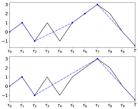
Figure 10. Top: The piecewise linear path $z^{m}$ with $m=10$ (black line) and the associated $y^{m}=\overline{\operatorname{orm}}_{m}[z]$ (blue dash-dotted line). Blue dots mark the value of $\overline{\operatorname{orm}}_{m}[z]$ at its interpolation points $\{\tau_{j(k)}\}_{k=0}^{\bar{m}}$. Bottom: The piecewise linear path $z^{m}$ (black line) and the associated $\tilde{y}^{m}$ computed by Algorithm 1 (blue dash-dotted line). Blue dots mark the value of $\tilde{y}^{m}$ at its interpolation points $\{\tilde{\tau}_{k}\}_{k=0}^{\tilde{L}(m)}$.

For later reference, note that the output mesh of Algorithm 1 satisfies $\{\tilde{\tau}_{k}\}_{k=0}^{\tilde{L}(m)-1}\subset A^{\pm}[z^{m}]$, and, using that for all $k<\tilde{L}(m)$,

$$y^{m}(\bar{A}^{+}[z^{m}](\tilde{\tau}_{k}))=M^{+}[z^{m}](\tilde{\tau}_{k})\quad\text{and}\quad y^{m}(\bar{A}^{-}[z^{m}](\tilde{\tau}_{k}))=M^{-}[z^{m}](\tilde{\tau}_{k}),$$

cf. Definition (4.15) and (4.16), it follows that $\{y^{m}(\bar{A}^{+}[z^{m}](\tilde{\tau}_{k}))\}_{k=0}^{\tilde{L}(m)-1}$ and
$\{y^{m}(\bar{A}^{-}[z^{m}](\tilde{\tau}_{k}))\}_{k=0}^{\tilde{L}(m)-1}$ respectively are monotonically increasing and decreasing sequences. For any $1\leq k\leq\tilde{L}(m)-2$ such that $\tilde{\tau}_{k}=\bar{A}^{+}[z^{m}](\tilde{\tau}_{k})$, it must hold that $\dot{y}^{m}(\tilde{\tau}_{k}+)<0$. Consequently, $\tilde{\tau}_{k+1}=\tau^{-}_{k}$, and since

$$y^{m}(\tilde{\tau}_{k+1})<y^{m}(\tilde{\tau}_{k})\leq y^{m}(\bar{A}^{+}[z^{m}](\tilde{\tau}_{k+1}))$$

implies that $\tilde{\tau}_{k+1}\neq\bar{A}^{+}[z^{m}](\tilde{\tau}_{k+1})$, it must hold that $\tilde{\tau}_{k+1}=\bar{A}^{-}[z^{m}](\tilde{\tau}_{k+1})$. By similar reasoning, if $1\leq k\leq\tilde{L}(m)-2$ is such that $\tilde{\tau}_{k}=\bar{A}^{-}[z^{m}](\tilde{\tau}_{k})$, then $\tilde{\tau}_{k+1}=\bar{A}^{+}[z^{m}](\tilde{\tau}_{k})$. We obtain that $\tilde{y}^{m}_{k}\tilde{y}^{m}_{k+1}\leq 0$ for all $k\leq\tilde{L}(m)-2$,

$$\tilde{y}^{m}_{k}\tilde{y}^{m}_{k+2}\geq 0\quad\text{and}\quad|\tilde{y}^{m}_{k}|\leq|\tilde{y}^{m}_{k+2}|\qquad\forall k\leq\tilde{L}(m)-3,$$

and as $\tilde{y}^{m}_{1}\neq 0$, if $\tilde{L}(m)>1$,

(4.53) $$\Delta\tilde{y}^{m}_{k}\Delta\tilde{y}^{m}_{k+1}<0\quad\text{and}\quad|\Delta\tilde{y}^{m}_{k}|\leq|\Delta\tilde{y}^{m}_{k+1}|\quad\forall k\leq\tilde{L}(m)-3.$$

(For the last index, $k=L(m)-2$, the properties (4.53) hold if $T\in A^{\pm}[z^{m}]$, but may not hold if $T\notin A^{\pm}[z^{m}]$.)

Corollary 4.11.

Assume $f\in C^{2}(\mathbb{R})$ is strictly convex, $u_{0}\in(L^{1}\cap BV)(\mathbb{R})$ and $z\in C_{0}([0,T])$. For any mesh $0=\tau_{0}<\tau_{1}<\ldots<\tau_{m}=T$, $m\geq 2$, let $y^{m}=\overline{\operatorname{orm}}_{m}[z]$ and $\tilde{y}^{m}=\mathcal{I}[y^{m}](\cdot;\{\tilde{\tau}_{k}\}_{k=0}^{\tilde{L}(m)})$, cf. Algorithm 1.

Then

(4.54) $$v(T;y^{m},\{\tau_{k}\}_{k=0}^{m})=v(T;\tilde{y}^{m},\{\tilde{\tau}_{k}\}_{k=0}^{\tilde{L}(m)})$$

and

(4.55) $${\left|y^{m}\right|}_{\mathrm{BV}([0,T])}={\left|\tilde{y}^{m}\right|}_{\mathrm{BV}([0,T])}.$$

Proof.

Equation (4.54) follows directly by Lemma 4.3.

To verify (4.55), note by Algorithm 1 that for any $k\in\{0,1,\ldots,\tilde{L}(m)-1\}$, it either holds that

$$\dot{y}^{m}(s+)\geq 0\quad\text{and}\quad\dot{\tilde{y}}^{m}(s+)\geq 0\quad\forall s\in[\tilde{\tau}_{k},\tilde{\tau}_{k+1}),$$

or

$$\dot{y}^{m}(s+)\leq 0\quad\text{and}\quad\dot{\tilde{y}}^{m}(s+)\leq 0\quad\forall s\in[\tilde{\tau}_{k},\tilde{\tau}_{k+1}),$$

and that

$$\tilde{y}^{m}(\tilde{\tau}_{k})=y^{m}(\tilde{\tau}_{k})\quad\forall k\in\{0,1,\ldots,\tilde{L}(m)\}.$$

Consequently,

$$\begin{split}{\left|y^{m}\right|}_{\mathrm{BV}([0,T])}&=\sum_{k=0}^{\bar{m}-1}{\left|y^{m}(\tau_{j(k+1)})-y^{m}(\tau_{j(k)})\right|}\\ &=\sum_{k=0}^{\tilde{L}(m)-1}{\left|y^{m}(\tilde{\tau}_{k+1})-y^{m}(\tilde{\tau}_{k})\right|}={\left|\tilde{y}^{m}\right|}_{\mathrm{BV}([0,T])}.\end{split}$$

∎

We now propose a numerical method that makes use of the piecewise linear orm function of $z$ and $\tilde{y}^{m}$ to compute entropy solutions at final time:

1. Approximate the rough path $z\in C_{0}([0,T])$ by the piecewise linear interpolant $z^{m}=\mathcal{I}^{m}[z]$ on a uniform mesh $\{\tau_{k}\}_{k=0}^{m}$ with step size $T/m$.

2. Compute $y^{m}=\overline{\operatorname{orm}}_{m}[z]$ and its interpolation points $\{\tau_{j(k)}\}_{k=0}^{\bar{m}}$, cf. Definition 4.3.

3. Compute $\tilde{y}^{m}$ and its interpolation points $\{\hat{\tau}_{k=0}\}_{k=0}^{\hat{L}(m)}$ by Algorithm 1 with $y^{m}$ and $\{\tau_{j(k)}\}_{k=0}^{\bar{m}}$ as input.

4. Compute a numerical solution of $v(T;\tilde{y}^{m},\{\tilde{\tau}_{k}\}_{k=0}^{\tilde{L}(m)})$, cf. (4.21) using a consistent, conservative and monotone finite volume method.

The numerical solution of $v\left(T;\tilde{y}^{m},\{\tau_{k}\}_{k=0}^{\tilde{L}(m)}\right)$, which we denote $U(T)$, is obtained through initializing $U(0)$ by (3.5), and iteratively, for $k=0,1,\ldots,\tilde{L}(m)-1$, computing the numerical solution of

(4.56) $$\begin{split}\partial_{t}\tilde{u}+\operatorname*{sign}\left(\Delta\tilde{y}^{m}_{k}\right)\partial_{x}f(\tilde{u})&=0\quad\text{in}\quad(0,|\Delta\tilde{y}^{m}_{k}|]\times\mathbb{R},\\ \quad\tilde{u}(0)&=U(\tilde{\tau}_{k}),\end{split}$$

and setting $U(\tilde{\tau}_{k+1})=\hat{\tilde{u}}(|\Delta\tilde{y}^{m}_{k}|;U(\tilde{\tau}_{k}))$, where $\hat{\tilde{u}}(s;U(\tilde{\tau}_{k}))$ denotes the numerical solution of (4.56) with $\hat{\tilde{u}}(0)=U(\tilde{\tau}_{k})$. We let $\tilde{n}(k)\geq 1$ denote the number of uniform timesteps used in the numerical solution of (4.56) over $[0,|\Delta\tilde{y}^{m}_{k}|]$, and

$$N=\sum_{k=0}^{\tilde{L}(m)-1}\tilde{n}(k),$$

denotes the total number of timesteps the numerical method uses to obtain the final time solution $U(T)$. The size of the uniform timesteps used in the numerical solution of the $k$-th problem (4.56), for $k\in\{0,1,\ldots,\tilde{L}(m)-1\}$, is determined through the following CFL condition:

(4.57) $$\begin{cases}\widetilde{\Delta}t_{k}=\frac{{\left|\Delta\tilde{y}^{m}_{k}\right|}}{\tilde{n}(k)},\quad\text{where}\\ \\ \tilde{n}(k)=\max\left(\left\lceil\frac{{\left|\Delta\tilde{y}^{m}_{k}\right|}\|f^{\prime}\|_{\infty}}{C_{\mathrm{CFL}}\Delta x}\right\rceil,\,1\right).\end{cases}$$

In other words, the numerical solution of the $k$-th problem  is computed on the temporal mesh discretization

(4.58) $$0=t_{k,0}\leq t_{k,1}\leq\ldots\leq t_{k,\tilde{n}(k)}=|\Delta\tilde{y}^{m}_{k}|,$$

where $t_{k,r}=r\widetilde{\Delta}t_{k}$ for $0\leq r\leq\tilde{n}(k)$.

For a given $z\in C_{0}^{0,\alpha}(\mathbb{R})$, $\alpha\in(0,1]$, Theorem 3.4 shows that the factors ${\left|z^{m}\right|}_{BV([0,T])}^{5}$ and ${\left|z^{m}\right|}_{BV([0,T])}^{6}$ respectively enter in lower and upper bounds of the computational cost of solving $v(T;z^{m},\{\tau_{k}\}_{k=0}^{m})$ by the adaptive time stepping method in Section 3. In comparison, the method considered here solves $v(T;\tilde{y}^{m},\{\tilde{\tau}_{k}\}_{k=0}^{\tilde{L}(m)})$, and since

$$|\tilde{y}^{m}|_{BV([0,T])}=|\overline{\operatorname{orm}}_{m}[z^{m}]|_{BV{([0,T])}}\leq{\left|z^{m}\right|}_{BV([0,T])}\quad\forall m\geq 2,$$

cf. Corollary 4.11, it is to be expected that the latter numerical method can be more efficient than the former. The following theorem states conditions under which efficiency gains are achieved.

Theorem 4.12.

Let $u\in C([0,T];L^{1}(\mathbb{R}))$ denote the unique pathwise entropy solution of (1.5) for given $u_{0}\in(L^{1}\cap BV)(\mathbb{R})$ with $\mathrm{Leb}\left(\mathrm{supp}\left(u_{0}\right)\right)>0$, strictly convex $f\in C^{2}(\mathbb{R})$ and $z\in C^{0,\alpha}_{0}([0,T])$ with $\alpha\in(0,1]$. For any $m\geq 2$, let $\{\tau_{j}\}_{j=0}^{m}\subset[0,T]$ denote the uniform mesh with step size $\Delta\tau=T/m$ and assume the computational cost of generating the interpolant $z^{m}=\mathcal{I}^{m}[z]$ is $\Theta(m^{\beta})$ for some $\beta\geq 1$. Set $y^{m}=\overline{\operatorname{orm}}_{m}[z]$, and let $\tilde{y}^{m}=\mathcal{I}[y^{m}]\left(\cdot;\{\tilde{\tau}_{k}\}_{k=0}^{\tilde{L}(m)}\right)$ denote the function generated by Algorithm 1. Let $U$ denote the solution of the numerical method in Section 4.3 satisfying the local CFL condition (4.57) and with the following constraint imposed on the spatial resolution

(4.59) $$\Delta x={\Theta}\!\left(\frac{\Delta\tau^{\alpha}}{\max\left(|y^{m}|_{BV([0,T])}^{2},\,1\right)}\right).$$

Assume that the spatial support of $U([0,T])$ is covered by an interval $[a_{m},b_{m}]\subset\mathbb{R}$ that satisfies

$$c_{1}\leq b_{m}-a_{m}\leq c_{2}(1+N\Delta x),$$

for some $c_{1},c_{2}>0$, cf. (3.10), and that at least one of the following two conditions hold:

• $$\tilde{L}(m)={\mathcal{O}}\!\left(m^{\alpha}\max\left(|y^{m}|_{BV([0,T])}^{3},1\right)\right),$$

• there exists an $\tilde{m}\geq 2$ and $\tilde{c}>0$ such that

  $$\max\left(M^{+}[z^{m}](\tau_{\left\lceil m^{\alpha}\right\rceil}),{\left|M^{-}[z^{m}](\tau_{\left\lceil m^{\alpha}\right\rceil})\right|}\right)\geq\tilde{c}m^{-\alpha}\qquad\forall m\geq\tilde{m}.$$

Then

(4.60) $$N=\sum_{k=0}^{\tilde{L}(m)-1}\widetilde{n}(k)={\mathcal{O}}\!\left(\frac{\max\left(|y^{m}|_{BV([0,T])}^{3},\,1\right)}{\Delta\tau^{\alpha}}\right),$$

and

$$\|u(T)-U(T)\|_{1}={\mathcal{O}}\!\left(m^{-\alpha/2}\right)$$

is achieved at the computational cost

$$\hat{c}_{1}\left(\max\left(|y^{m}|_{BV([0,T])}^{5},\,1\right)m^{2\alpha}+m^{\beta}\right)\\ \leq\mathrm{Cost}(U)\leq\\ \hat{c}_{2}\left(\max\left(|y^{m}|_{BV([0,T])}^{6},\,1\right)m^{2\alpha}+m^{\beta}\right),$$

for some $\hat{c}_{1},\hat{c}_{2}>0$.

Proof.

By the CFL condition (4.57), it holds for all $m\geq 2$ that

$$\max_{k\in\{0,1,\ldots,\tilde{L}(m)-1\}}\widetilde{\Delta}t_{k}\leq\frac{C_{\mathrm{CFL}}}{\|f^{\prime}\|_{\infty}}\Delta x.$$

Introducing the shorthand

$$\tilde{v}^{m}(\tilde{\tau}_{k})\mathrel{\vbox{\hbox{\scriptsize.}\hbox{\scriptsize.}}}=v\left(\tilde{\tau}_{k};\tilde{y}^{m},\{\tilde{\tau}_{k}\}_{k=0}^{\tilde{L}(m)}\right)\qquad\forall k\in\{0,1,\ldots,\tilde{L}(m)\},$$

and using Kuznetsov’s lemma, cf. [49, Example 3.15], the error of the numerical method at time $\tilde{\tau}_{k+1}$ can be bounded by

(4.61) $$\begin{split}\|\tilde{v}^{m}(\tilde{\tau}_{k+1})-U(\tilde{\tau}_{k+1})\|_{1}&\leq\|\tilde{v}^{m}(\tilde{\tau}_{k})-U(\tilde{\tau}_{k})\|_{1}+C|\Delta\tilde{y}^{m}_{k}|(\sqrt{\widetilde{\Delta}t_{k}}+\sqrt{\Delta x})\\ &\leq\|\tilde{v}^{m}(\tilde{\tau}_{k})-U(\tilde{\tau}_{k})\|_{1}+C|\Delta\tilde{y}^{m}_{i}|\sqrt{\Delta x},\end{split}$$

for some $C>0$ that depends on $\|f^{\prime}\|_{L^{\infty}}$, $|u_{0}|_{BV(\mathbb{R})}$ and the numerical scheme. Using that $\tilde{v}^{m}(0)=u_{0}$, $\tilde{v}^{m}(T)=u^{m}(T)$ and $|\tilde{y}^{m}|_{BV([0,T])}=|y^{m}|_{BV([0,T])}$, cf. Corollary 4.11 and Theorem 4.5, we obtain

$$\|u^{m}(T)-U(T)\|_{1}\leq\|u_{0}-U(0)\|_{1}+C|y^{m}|_{BV([0,T])}\sqrt{\Delta x}.$$

By Theorem 2.1, (4.61), and (4.59),

(4.62) $$\begin{split}\|u(T)-U(T)\|_{1}&\leq\|u(T)-u^{m}(T)\|_{1}+\|u^{m}(T)-U(T)\|_{1}\\ &={\mathcal{O}}\!\left(\Delta\tau^{\alpha/2}+|y^{m}|_{BV([0,T])}\sqrt{\Delta x}\right)\\ &={\mathcal{O}}\!\left(\Delta\tau^{\alpha/2}\right).\end{split}$$

And by (4.57) and (4.59),

$$\begin{split}N&=\sum_{k=0}^{\tilde{L}(m)-1}\tilde{n}(k)\leq\sum_{k=0}^{\tilde{L}(m)-1}\left(\frac{{\left|\Delta\tilde{y}^{m}_{k}\right|}\|f^{\prime}\|_{L^{\infty}}}{C_{\mathrm{CFL}}\Delta x}+1\right)\\ &\leq\frac{\|f^{\prime}\|_{L^{\infty}}}{C_{\mathrm{CFL}}\Delta x}{\left|y^{m}\right|}_{BV([0,T])}+\tilde{L}(m)\\ &={\mathcal{O}}\!\left(m^{\alpha}\max\left({\left|y^{m}\right|}_{BV([0,T])}^{3},\,1\right)+\tilde{L}(m)\right).\end{split}$$

In order to obtain (4.60), it remains to verify that

(4.63) $$\tilde{L}(m)={\mathcal{O}}\!\left(m^{\alpha}\max\left(|y^{m}|_{BV([0,T])}^{3},\,1\right)\right).$$

Assume condition (b) holds and that $m\geq\tilde{m}$. Since $\{\tilde{\tau}_{k}\}_{k=0}^{\tilde{L}(m)-1}\subset A^{\pm}[z^{m}]$ and $\{|\Delta\tilde{y}^{m}_{k}|\}_{k=0}^{\tilde{L}(m)-2}$ is a monotonically increasing sequence, cf. (4.53), it holds for any $\tau_{r}\in\{\tilde{\tau}_{k}\}_{k=0}^{\tilde{L}(m)-2}\cup[\tau_{\left\lceil m^{\alpha}\right\rceil},T)$ that

$$|\Delta\tilde{y}^{m}_{r}|\geq\max\left(M^{+}[z^{m}](\tilde{\tau}_{r}),{\left|M^{-}[z^{m}](\tilde{\tau}_{r})\right|}\right)\geq\tilde{c}m^{-\alpha}.$$

Moreover, the following function is well-defined for all $m\geq\tilde{m}$:

$$r(m)\mathrel{\vbox{\hbox{\scriptsize.}\hbox{\scriptsize.}}}=\min\Big{\{}k\in\{0,1,\ldots,\left\lceil m^{\alpha}\right\rceil\}\mid|\Delta\tilde{y}^{m}_{k}|>\tilde{c}m^{-\alpha}\Big{\}}.$$

It is clear that $r(m)={\mathcal{O}}\!\left(m^{\alpha}\right)$ and

$$\begin{split}|\tilde{y}^{m}|_{BV([0,T])}&=\sum_{k=0}^{\tilde{L}(m)-1}|\Delta\tilde{y}^{m}_{k}|\geq\sum_{k=r(m)}^{\tilde{L}(m)-2}m^{-\alpha}=(\tilde{L}(m)-(r(m)+2))m^{-\alpha}.\end{split}$$

We conclude that

$$\tilde{L}(m)={\mathcal{O}}\!\left(m^{\alpha}\max\left(|y^{m}|_{BV([0,T])},\,1\right)\right)={\mathcal{O}}\!\left(m^{\alpha}\max\left(|y^{m}|_{BV([0,T])}^{3},\,1\right)\right),$$

and thus condition (b) is stronger than condition (a) (condition (b) is included in the theorem as it might be easier to verify than condition (a)).

The computational cost of the numerical method is equal to the sum of ${\Theta}\!\left(m^{\beta}\right)$ for generating the piecewise linear interpolant $z^{m}$, and

$$\begin{split}{\Theta}\!\left(N\times\frac{b_{m}-a_{m}}{\Delta x}\right)\end{split}$$

for solving $U$ over $[0,T]\times[a_{m},b_{m}]$. ∎

4.4. Efficiency gains

By comparing the computational cost versus accuracy results in Theorems 3.4 and 4.12, we see that if the assumptions of both theorems hold,

$$\limsup_{m\to\infty}\frac{m^{\beta}}{m^{2\alpha}|z^{m}|^{5}_{BV([0,T])}}=0,$$

and

(4.64) $$\limsup_{m\to\infty}\frac{|\overline{\operatorname{orm}}_{m}[z]\,|_{BV([0,T])}^{6}}{{\left|z^{m}\right|}_{BV([0,T])}^{5}}=0,$$

then it is guaranteed that the orm based numerical method will asymptotically be more efficient than the adaptive timestep method.

The next two lemmas, Lemmas 4.13 and 4.14, verify that ${\left|\overline{\operatorname{orm}}_{m}[z]\right|}_{BV([0,T])}<\infty$, for all $m\geq 2$, and assumption (b) in Theorem 4.12 hold for almost all sample paths of a standard Wiener process.

Lemma 4.13.

Let $(\Omega,\mathcal{F},\mathbb{P})$ denote a probability space on which the standard Wiener process $W:[0,\infty)\times\Omega\to\mathbb{R}$ with $W(0)=0$, $\mathbb{P}$-a.s. is defined. For every $\omega\in\Omega$, let $z\mathrel{\vbox{\hbox{\scriptsize.}\hbox{\scriptsize.}}}=W(\cdot,\omega)$ denote a sample path of the Wiener process. Then, for every $\alpha\in(0,1/2)$ and $\widehat{T}>0$

(4.65) $$z\in C_{0}^{0,\alpha}([0,\widehat{T}]),\qquad\mathbb{P}\mathrm{-a.s.}$$

Furthermore, for a fixed $T>0$, let

(4.66) $$\widetilde{\Omega}=\{\omega\in\Omega\mid W(\cdot,\omega)\in C_{0}([0,T])\},$$

and for any $m\geq 2$, let $\{\tau_{k}\}_{k=0}^{m}\subset[0,T]$ denote the uniform mesh with step size $\Delta\tau=T/m$. We define

(4.67) $$z^{m}\mathrel{\vbox{\hbox{\scriptsize.}\hbox{\scriptsize.}}}=\begin{cases}\mathcal{I}[z](\cdot;\{\tau_{k}\}_{k=0}^{m})&\text{if}\quad\omega\in\widetilde{\Omega},\\ 0&\text{if}\quad\omega\in\Omega\setminus\widetilde{\Omega},\end{cases}$$

and

(4.68) $$\overline{\operatorname{orm}}_{m}[z]\mathrel{\vbox{\hbox{\scriptsize.}\hbox{\scriptsize.}}}=\begin{cases}\overline{\operatorname{orm}}[z](\cdot;\{\tau_{k}\}_{k=0}^{m})&\text{if}\quad\omega\in\widetilde{\Omega},\\ 0&\text{if}\quad\omega\in\Omega\setminus\widetilde{\Omega}.\end{cases}$$

Then

(4.69) $$\limsup_{m\to\infty}\sup_{t\in[0,T]}|z-z^{m}|(t)\sqrt{\frac{m}{\log(m)}}\leq\sqrt{2T},\qquad\mathbb{P}\mathrm{-a.s.,}$$

(4.70) $$\limsup_{m\to\infty}{\left|z^{m}\right|}_{BV([0,T])}\sqrt{\frac{\log(m)}{m}}\geq\sqrt{\frac{T}{2}},\quad\mathbb{P}\mathrm{-a.s.,}$$

and for $\mathbb{P}$-almost all paths, there is a constant $C(\omega)>0$ such that

(4.71) $$\limsup_{m\to\infty}{\left|\overline{\operatorname{orm}}_{m}[z]\right|}_{BV([0,T])}<C(\omega).$$

Moreover,

(4.72) $${\mathbb{E}\mspace{-2.0mu}\left[\sup_{m\geq 2}{\left|\overline{\operatorname{orm}}_{m}[z]\right|}_{BV([0,T])}\right]}<\infty,\quad{\mathbb{E}\mspace{-2.0mu}\left[{\left|\operatorname{orm}[z]\right|}_{BV([0,T])}\right]}<\infty.$$

Proof.

See [29] for a proof of (4.65).

Since $\mathbb{P}\mspace{-2.0mu}\left(\widetilde{\Omega}\right)=1$, we restrict ourselves to $\omega\in\widetilde{\Omega}$ in what follows. By Lévy’s global modulus of continuity [51, Theorem 9.25] ,

$$\limsup_{\delta\downarrow 0}\sup_{{\scriptsize\begin{split}0&\leq s\leq t\leq T\\ &t-s\leq\delta\end{split}}}\frac{{\left|z(t)-z(s)\right|}}{\sqrt{2\delta\log(1/\delta)}}=T,\qquad\mathbb{P}\mathrm{-a.s.,}$$

and as

$$\begin{split}\sup_{t\in[0,T]}{\left|z(t)-z^{m}(t)\right|}&\leq\max_{k\in\{0,1,\ldots,m-1\}}\sup_{t\in[\tau_{k},\tau_{k+1}]}\max\left({\left|z(t)-z(\tau_{k})\right|},{\left|z(t)-z(\tau_{k+1)}\right|}\right)\\ &\leq\sup_{{\scriptsize\begin{split}0&\leq s\leq t\leq T\\ &t-s\leq T/m\end{split}}}{\left|z(t)-z(s)\right|},\end{split}$$

inequality (4.69) follows and so does

$$\limsup_{m\to\infty}\left(\max_{k\in\{0,1,\ldots,m-1\}}{\left|\Delta z^{m}_{k}\right|}\sqrt{\frac{m}{\log(m)}}\right)\leq\sqrt{2T},\qquad\mathbb{P}\mathrm{-a.s.}$$

We further recall from [25] that

$$\limsup_{m\to\infty}\sum_{k=1}^{m-1}{\left|\Delta z^{m}_{k}\right|}^{2}=\lim_{m\to\infty}\sum_{k=1}^{m-1}{\left|\Delta z^{m}_{k}\right|}^{2}=T,\qquad\mathbb{P}\mathrm{-a.s.}$$

Hence,

$$\begin{split}T&=\limsup_{m\to\infty}\sum_{k=1}^{m-1}{\left|\Delta z^{m}_{k}\right|}^{2}\\ &\leq\limsup_{m\to\infty}\left(\max_{\ell\in\{0,1,\ldots,m-1\}}{\left|\Delta z^{m}_{\ell}\right|}\sum_{k=1}^{m-1}{\left|\Delta z^{m}_{k}\right|}\right)\\ &\leq\limsup_{m\to\infty}\left(\max\left(\max_{k\in\{0,1,\ldots,m-1\}}{\left|\Delta z^{m}_{k}\right|}\sqrt{\frac{m}{\log(m)}},\,\sqrt{2T}\right)\right)\\ &\qquad\times\limsup_{m\to\infty}\left({\left|z^{m}\right|}_{BV([0,T])}\sqrt{\frac{\log(m)}{m}}\right)\\ &=\sqrt{2T}\limsup_{m\to\infty}\left({\left|z^{m}\right|}_{BV([0,T])}\sqrt{\frac{\log(m)}{m}}\right),\qquad\qquad\mathbb{P}\mathrm{-a.s.},\end{split}$$

and (4.70) follows.

Equations (4.71) and (4.72) are proved in Appendix B. ∎

The next lemma shows that assumption (b) in Theorem 4.12 holds for almost all sample paths of a standard Wiener process.

Lemma 4.14.

For any $m\geq 2$, let $\{\tau_{k}\}_{k=0}^{m}\subset[0,T]$ denote the uniform mesh with with step size $\Delta\tau=T/m$. Let $z=W(\cdot,\omega)\in C_{0}([0,T])$ denote a path realization of the standard Wiener process with $\omega\in\widetilde{\Omega}$, cf. Lemma 4.13 and (4.66), and let $z^{m}$ be defined by (4.67). Then, for any $\alpha\in(2/5,1]$, there exists an $\tilde{m}(\omega)\geq 2$ for almost all $\omega\in\widetilde{\Omega}$ such that

(4.73) $$\max\left(M^{+}[z^{m}](\tau_{\left\lceil m^{\alpha}\right\rceil}),{\left|M^{-}[z^{m}](\tau_{\left\lceil m^{\alpha}\right\rceil})\right|}\right)\geq m^{-\alpha}\qquad\forall m\geq\tilde{m}(\omega).$$

Proof.

For $y\in\mathbb{R}$, let $\left\lfloor y\right\rfloor$ denote the largest $n\in\mathbb{Z}$ such that $y\geq n$ and let $r^{m}:\mathbb{N}\to\mathbb{N}$ be defined by $r^{m}(k)=\left\lfloor m^{\alpha/2}\right\rfloor k$. For any natural number $m\geq\hat{m}=\left\lceil 3^{2/\alpha}\right\rceil$, we introduce the set

$$\begin{split}D_{m}=\left\{\omega\in\tilde{\Omega}\,\Big{|}\,\,{\left|z(\tau_{r^{m}(k+1)})-z(\tau_{r^{m}(k)})\right|}\leq\frac{2}{m^{\alpha}}\quad\text{for}\quad k=0,1,\ldots,\left\lfloor m^{\alpha/2}\right\rfloor-1\right\}.\end{split}$$

We claim that $\omega\in\widetilde{\Omega}$ for which (4.73) does not hold is contained in

(4.74) $$\bigcap_{m\geq\hat{m}}\bigcup_{\ell\geq m}D_{\ell}.$$

To verify this, observe that if $\omega\notin\bigcap_{m\geq\hat{m}}\bigcup_{\ell\geq m}D_{\ell}$, then there exists an $\tilde{m}(\omega)$ such that $\omega\notin\bigcup_{\ell\geq\tilde{m}}D_{\ell}$. Since $\omega\notin D_{m}$ for every $m\geq\tilde{m}$, there exists a $k_{m}\in\{0,1,\ldots,\left\lfloor m^{\alpha/2}\right\rfloor-1\}$ such that ${\left|z(\tau_{r^{m}(k_{m}+1)})-z(\tau_{r^{m}(k_{m})})\right|}\geq\frac{2}{m^{\alpha}}$. This implies that $\max(|z(\tau_{r^{m}(k_{m}+1)})|,|z(\tau_{r^{m}(k_{m})})|)>m^{-\alpha}$, and, since $r^{m}(k_{m}+1)\leq\left\lceil m^{\alpha}\right\rceil$ by construction, we conclude that

$$\max\left(M^{+}[z^{m}](\tau_{\left\lceil m^{\alpha}\right\rceil}),{\left|M^{-}[z^{m}](\tau_{\left\lceil m^{\alpha}\right\rceil})\right|}\right)\geq m^{-\alpha},\qquad\forall m\geq\tilde{m}.$$

We will show that (4.74) is a zero-measure set. Since the increments $\{z(\tau_{r^{m}(k+1)})-z(\tau_{r^{m}(k)})\}_{k}$ are independent $N\left(0,\tau_{\left\lfloor m^{\alpha/2}\right\rfloor}\right)$ distributed random variables,

$$\mathbb{P}\mspace{-2.0mu}\left(D_{m}\right)\leq\left(\mathbb{P}\mspace{-2.0mu}\left({\left|z(\tau_{r^{m}(1)})-z(0)\right|}\leq\frac{2}{m^{\alpha}}\right)\right)^{\left\lfloor m^{\alpha/2}\right\rfloor},$$

and since $\tau_{\left\lfloor r^{m}(1)\right\rfloor}={\Theta}\!\left(m^{\alpha/2-1}\right)$, there exists a $C>0$ independent of $m$ such that for all $m\geq\hat{m}$,

$$\begin{split}\mathbb{P}\mspace{-2.0mu}\left({\left|z(\tau_{r^{m}(1)})-z(0)\right|}\leq\frac{2}{m^{\alpha}}\right)&=\frac{1}{\sqrt{2\pi\tau_{r^{m}(1)}}}\int_{-2m^{-\alpha}}^{2m^{-\alpha}}\exp\left(\frac{-x^{2}}{2\tau_{r^{m}(1)}}\right)\,\mathrm{d}x\\ &=\frac{1}{\sqrt{2\pi}}\int_{\frac{-2m^{-\alpha}}{\sqrt{\tau_{r^{m}(1)}}}}^{\frac{2m^{-\alpha}}{\sqrt{\tau_{r^{m}(1)}}}}e^{-y^{2}/2}\,\mathrm{d}y\\ &\leq Cm^{1/2-5\alpha/4}.\end{split}$$

Since $1/2-5\alpha/4<0$, there exists a $\check{m}\geq\hat{m}$, such that

$$\mathbb{P}\mspace{-2.0mu}\left(D_{m}\right)\leq m^{-2}\quad\text{for all}\quad m\geq\check{m},$$

and

$$\mathbb{P}\mspace{-2.0mu}\left(\bigcap_{m\geq\hat{m}}\bigcup_{\ell\geq m}D_{\ell}\right)\leq\liminf_{m\to\infty}\mathbb{P}\mspace{-2.0mu}\left(\bigcup_{\ell\geq m}D_{\ell}\right)\leq\liminf_{m\to\infty}\sum_{\ell=m}^{\infty}\mathbb{P}\mspace{-2.0mu}\left(D_{\ell}\right)\leq\lim_{m\to\infty}\frac{1}{m}=0.$$

Equations (4.65) and (4.66) ensures that

$$\mathbb{P}\mspace{-2.0mu}\left(\widetilde{\Omega}\setminus\bigcap_{m\geq\hat{m}}\bigcup_{\ell\geq m}D_{\ell}\right)=1,$$

and the proof follows. ∎

By the “Hölder continuity” (4.69), equations (4.70) and (4.71), and the fact that $\beta=1$ for sampling a path of a standard Wiener processes, we conclude that under the shared assumptions on $u_{0}$ in Theorems 3.4 and 4.12 and if $f\in C^{2}(\mathbb{R})$ is strictly convex, then the computational cost of achieving

$$\|u(T)-U(T)\|_{L^{1}}={\mathcal{O}}\!\left(\left(\frac{\log(m)}{m}\right)^{1/4}\right),$$

for a sample path $z:[0,T]\to\mathbb{R}$ of the standard Wiener process admits for some $c_{1}(\omega)>0$ the following lower bound for the adaptive time stepping method (cf. Theorem 3.4):

$$\mathrm{Cost}(U(T))\geq c_{1}\left(\frac{m}{\log(m)}\right)^{7/2}\qquad\mathbb{P}\mathrm{-a.s.,}$$

and, for some $c_{2}(\omega)>0$, the following upper bound for the orm based method (cf. Theorem 4.12):

$$\mathrm{Cost}(U(T))\leq c_{2}m\qquad\mathbb{P}\mathrm{-a.s.}$$

Remark 4.2.

In many cases (e.g. Brownian paths), ${\left|\operatorname{orm}[z]\right|}_{BV([0,T])}<{\left|z\right|}_{BV([0,T])}$. That is however not always the case. The second example in Figure 9 considers the locally rough path $z(t)={\mathbf{1}_{t>0}}t\sin(\pi/(2t))$, which is a member of $C^{0,1/2}_{0}([0,T])$ for which ${\left|\operatorname{orm}[z]\right|}_{BV([0,T])}={\left|z\right|}_{BV([0,T])}=\infty$. This shows that even if $f\in C^{2}(\mathbb{R})$ is strictly convex, the orm based method will not always solve (1.5) more efficiently than the adaptive timestepping method.

4.5. Numerical tests

Example 4.1.

To investigate if Lemma 4.13 holds more generally, we approximate ${\mathbb{E}\mspace{-2.0mu}\left[{\left|z^{m}\right|}_{BV([0,1])}\right]}$ and ${\mathbb{E}\mspace{-2.0mu}\left[{\left|\overline{\operatorname{orm}}_{m}[z]\right|}_{BV([0,1])}\right]}$ for four different fBMs with respective Hurst indices $\alpha=1/8,1/4,1/2$ and $3/4$ on uniform meshes of $[0,1]$ with respective step sizes $\Delta\tau=1/m$ for $m=2^{5},2^{6},\ldots,2^{16}$. The expectations are approximated by the Monte Carlo method using $10^{6}$ sample realizations of ${\left|z^{m}\right|}_{BV([0,1])}$ and ${\left|\overline{\operatorname{orm}}_{m}[z]\right|}_{BV([0,1])}$.

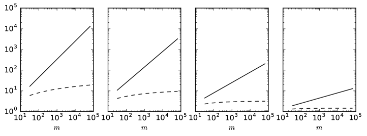
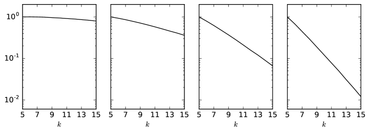
Figure 11. Top row: Example 4.1, Monte Carlo computations of ${\mathbb{E}\mspace{-2.0mu}\left[{\left|z^{m}\right|}_{BV([0,1])}\right]}$ (solid line) and ${\mathbb{E}\mspace{-2.0mu}\left[{\left|\overline{\operatorname{orm}}_{m}[z]\right|}_{BV([0,1])}\right]}$ (dashed line), Hurst indices $\alpha=0.125$ (left), $\alpha=0.25$ (second left), $\alpha=0.5$ (third left), and $\alpha=0.75$ (right). Bottom row: plots of the BV increment ratio $G(k)$, cf. (4.75), corresponding to the respective top row test cases.

Our Monte Carlo estimates of the expectations are presented in Figure 11. We observe that while ${\mathbb{E}\mspace{-2.0mu}\left[{\left|z^{m}\right|}_{BV([0,1])}\right]}={\Theta}\!\left(m^{1-\alpha}\right)$, ${\mathbb{E}\mspace{-2.0mu}\left[|\overline{\operatorname{orm}}_{m}[z]|_{BV([0,1])}\right]}$ seems to stay bounded as $m$ increases for all of the considered fBMs. In the bottom row of Figure 11, we have computed the “BV increment ratio”

(4.75) $$G(k):=\frac{{\mathbb{E}\mspace{-2.0mu}\left[|\overline{\operatorname{orm}}_{{}^{2^{k+1}}}[z]|_{BV([0,1])}-|\overline{\operatorname{orm}}_{2^{k}}[z]|_{BV([0,1])}\right]}}{{\mathbb{E}\mspace{-2.0mu}\left[|\overline{\operatorname{orm}}_{2^{6}}[z]|_{BV([0,1])}-|\overline{\operatorname{orm}}_{2^{5}}[z]|_{BV([0,1])}\right]}},$$

for $k\geq 5$. The increment ratio seems to be geometric of the form $G(k)={\mathcal{O}}\!\left(\rho_{\alpha}^{k-5}\right)$ with $\rho_{\alpha}\approx 2^{-\alpha}<1$. We interpret this as numerical support for

$${\mathbb{E}\mspace{-2.0mu}\left[\lim_{k\to\infty}|\overline{\operatorname{orm}}_{2^{k}}[z]|_{BV([0,1])}\right]}<\infty,\quad\forall\alpha\in\{1/8,1/4,1/2,3/4\},$$

since if $G(k)<1$,

$$\begin{split}&{\mathbb{E}\mspace{-2.0mu}\left[\lim_{k\to\infty}|\overline{\operatorname{orm}}_{2^{k}}[z]|_{BV([0,1])}\right]}\\ &={\mathbb{E}\mspace{-2.0mu}\left[|\overline{\operatorname{orm}}_{2^{5}}[z]|_{BV([0,1])}\right]}+\sum_{k=5}^{\infty}{\mathbb{E}\mspace{-2.0mu}\left[|\overline{\operatorname{orm}}_{2^{k+1}}[z]|_{BV([0,1])}-|\overline{\operatorname{orm}}_{2^{k}}[z]|_{BV([0,1])}\right]}\\ &\leq C\sum_{k=0}^{\infty}\rho_{\alpha}^{k}<\infty.\end{split}$$

Example 4.2.

We consider problem (3.19) over the time interval $[0,1]$ with periodic boundary conditions, initial data

$$u_{0}(x)=\operatorname*{sign}\left(x-1/2\right){\mathbf{1}_{1/6<5/6}}\qquad x\in[0,1],$$

strictly convex flux $f(u)=u/2+u^{2}/4$ and $z=W(\cdot,\omega)$, where $W:[0,1]\times\widetilde{\Omega}\to\mathbb{R}$ denotes the standard Wiener process and $\widetilde{\Omega}$ is defined in (4.66). In Figure 12 we compare the performance of the adaptive timestep method and the orm based method (cf. Section 4.3), both using the Lax–Friedrichs scheme. The driving path $z$ is piecewise linearly interpolated on two uniform mesh resolutions, $m=2^{8}$ and $m=2^{10}$, and the computational cost of the respective algorithms are equilibrated through

$$\Delta x_{\text{orm}}=\frac{\Delta x_{\mathrm{adaptive}}}{\left\lceil\sqrt{\frac{{\left|z^{m}\right|}_{BV([0,T])}}{|\operatorname{orm}[z^{m}]|_{BV([0,T])}}}\,\,\right\rceil},$$

(equilibrating either lower or upper bound costs in both of Theorems 3.4 and 4.7). The approximate reference solution is computed by the orm based method using the Lax–Friedrichs scheme with piecewise linear interpolation of $z$ on a uniform mesh with much higher resolution ($m=2^{14}$). We observe that at comparable computational budget, the orm based method approximates the reference solution with better accuracy and produces less artificial diffusion than the adaptive timestep method.

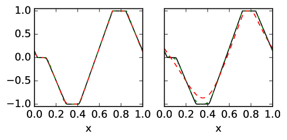
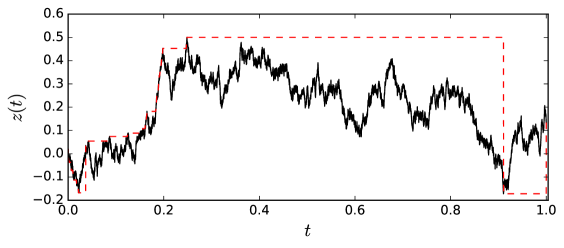
Figure 12. Top row: Final time solutions for Example 4.2 computed with the orm based method (left figure) and adaptive timestep method (right figure). The black solid line is the approximate reference solution $u(1)$, while the red dashed and the green dash-dotted lines are the numerical solutions at the rough path resolutions $m=2^{8}$ and $m=2^{10}$, respectively. Bottom: The rough path (black solid line) and the corresponding orm (red dashed line).

5. Conclusion

In this work we have developed fully discrete and thus computable numerical methods for solving conservation laws with rough paths. For strictly convex flux functions, we have identified a class of “oscillatory cancellations” that can be removed from the rough path to produce numerical methods with improved efficiency. If the rough path is a realization of a Wiener process, for instance, the asymptotic efficiency gain can be of orders of magnitude. An in-depth study of the rough path cancellation property is found in the theoretical companion article [44].

Appendix A Regularity of solutions

Lemma A.1.

For a given set of points

$$0=\tau_{0}<\tau_{1}<\ldots<\tau_{m}=T,\qquad m\geq 2,$$

let $u^{m}\in C_{0}([0,T];L^{1}(\mathbb{R}))$ denote the càdlàg version of the entropy solution of (2.1) with initial data $u_{0}\in(L^{1}\cap BV)(\mathbb{R})$, driving noise $z^{m}\in I_{0}([0,T];\{\tau_{j}\}_{j=0}^{m})$ and strictly convex $f\in C^{2}(\mathbb{R})$. For any $x\in\mathbb{R}$ and $t\in[0,T]$, let

$$u^{m}(t,x+)\mathrel{\vbox{\hbox{\scriptsize.}\hbox{\scriptsize.}}}=\lim_{\delta\downarrow 0}u^{m}(t,x+\delta)\,(=u(t,x))\quad\text{and}\quad u^{m}(t,x-)\mathrel{\vbox{\hbox{\scriptsize.}\hbox{\scriptsize.}}}=\lim_{\delta\downarrow 0}u^{m}(t,x-\delta),$$

Then, using the convention $0^{-1}=\infty$, it holds for all $x<y$ and $t\in[0,T]$ that

(A.1) $$\begin{split}-\frac{1}{M^{+}[z^{m}](t)-z^{m}(t)}&\leq\frac{f^{\prime}(u^{m}(t,y\pm))-f^{\prime}(u^{m}(t,x\pm))}{y-x}\leq\frac{1}{z^{m}(t)-M^{-}[z^{m}](t)},\end{split}$$

where the functions $M^{-}[z^{m}]$ and $M^{+}[z^{m}]$ are defined in (4.11).

To prove Corollary 4.2 we will need the following intermediate result, which is an adaptation of [44, Lemma 3.3].

Lemma A.2.

For a given set of points

$$0=\tau_{0}<\tau_{1}<\ldots<\tau_{m}=T,\qquad m\geq 2,$$

let $u^{m}\in C_{0}([0,T];L^{1}(\mathbb{R}))$ denote the càdlàg version of the entropy solution of (2.1) with initial data $u_{0}\in(L^{1}\cap BV)(\mathbb{R})$, driving noise $z^{m}\in I_{0}([0,T];\{\tau_{j}\}_{j=0}^{m})$ and strictly convex $f\in C^{2}(\mathbb{R})$. Assume that (A.1) holds at some time $\tau_{k}\in\{\tau_{j}\}_{j=0}^{m-1}$. Then, for all $x<y$ and $s\in[\tau_{k},\tau_{k+1}]$,

(A.2) $$\begin{split}-\frac{1}{M^{+}[z^{m}](s)-z^{m}(s)}&\leq\frac{f^{\prime}(u^{m}(s,y\pm))-f^{\prime}(u(s,x\pm))}{y-x}\leq\frac{1}{z^{m}(s)-M^{-}[z^{m}](s)}.\end{split}$$

Proof.

For some $s\in(\tau_{k},\tau_{k+1}]$, let $\zeta_{\pm}$ be the maximal/minimal backward generalized characteristic emanating from $(s,y)$ and $\xi_{\pm}$ be the maximal/minimal backward generalized characteristic emanating from $(s,x)$, cf. [18, § X]. The solution representation

$$u^{m}(s)=\bar{}\mathcal{S}(z^{m}(s)-z^{m}(\tau_{k}))u^{m}(\tau_{k})=\mathcal{S}^{\dot{z}^{m}_{k}}(s-\tau_{k})u^{m}(\tau_{k}),$$

cf. (3.2) and (4.4), and [18, Theorem 11.1.1] implies that the generalized characteristics satisfies the following equations

$$x =\xi_{\pm}(\tau_{k})+(s-\tau_{k})\dot{z}^{m}_{k}f^{\prime}(u^{m}(s,x\pm))=\xi_{\pm}(\tau_{k})+(z^{m}(s)-z^{m}(\tau_{k}))f^{\prime}(u^{m}(s,x\pm)),$$

$$y =\zeta_{\pm}(\tau_{k})+(s-\tau_{k})\dot{z}^{m}_{k}f^{\prime}(u^{m}(s,y\pm))=\zeta_{\pm}(\tau_{k})+(z^{m}(s)-z^{m}(\tau_{k}))f^{\prime}(u^{m}(s,y\pm)),$$

where $\xi_{\pm}(\tau_{k})\leq\zeta_{\pm}(\tau_{k})$ and each equation holds using either the limit sign $+$ or $-$ consistently in all terms with the appendage $\pm$ (i.e., $x+$ and $\xi_{+}(\tau_{k})$ etc.); and we recall that $\dot{z}^{m}_{k}=\dot{z}^{m}(\tau_{k}+)$. We will treat the cases $\dot{z}^{m}_{k}>0$ and $\dot{z}^{m}_{k}<0$ separately (the case $\dot{z}^{m}_{k}=0$ is trivial since then $u^{m}(t)=\mathcal{S}^{0}(t-\tau_{k})u^{m}(\tau_{k})=u^{m}(\tau_{k})$ for all $t\in[\tau_{k},\tau_{k+1}]$).

Assume $\dot{z}^{m}_{k}>0$. By [18, Theorem 11.1.3],

(A.3) $$\begin{split}u^{m}(\tau_{k},\xi_{\pm}(\tau_{k})-)&\leq u^{m}(s,x\pm)\leq u^{m}(\tau_{k},\xi_{\pm}(\tau_{k})+),\\ u^{m}(\tau_{k},\zeta_{\pm}(\tau_{k})-)&\leq u^{m}(s,y\pm)\leq u^{m}(\tau_{k},\zeta_{\pm}(\tau_{k})+).\end{split}$$

Under the assumption that $f^{\prime}(u^{m}(s,y\pm))-f^{\prime}(u^{m}(s,x\pm))\neq 0$ (otherwise (A.2) holds trivially), we have

(A.4) $$\begin{split}\frac{f^{\prime}(u^{m}(s,y\pm))-f^{\prime}(u(s,x\pm))}{y-x}=\frac{1}{\frac{\zeta_{\pm}(\tau_{k})-\xi_{\pm}(\tau_{k})}{f^{\prime}(u^{m}(s,y\pm))-f^{\prime}(u(s,x\pm))}+(z^{m}(s)-z^{m}(\tau_{k}))}.\end{split}$$

If $f^{\prime}(u^{m}(s,y\pm))-f^{\prime}(u^{m}(s,x\pm))<0$, then the upper bound of (A.2) holds trivially, and inequalities (A.3) and $f^{\prime}>0$ implies that

$$0>f^{\prime}(u^{m}(s,y\pm))-f^{\prime}(u^{m}(s,x\pm))\geq f^{\prime}(u^{m}(\tau_{k},\zeta_{\pm}(\tau_{k})-))-f^{\prime}(u^{m}(s,\xi_{\pm}(\tau_{k})+)).$$

Hence, either $\zeta_{\pm}(\tau_{k})=\xi_{\pm}(\tau_{k})$ or $\zeta_{\pm}(\tau_{k})>\xi_{\pm}(\tau_{k})$. In the former case, the lower bound of (A.2) holds since

$$\frac{\zeta_{\pm}(\tau_{k})-\xi_{\pm}(\tau_{k})}{f^{\prime}(u^{m}(s,y\pm))-f^{\prime}(u(s,x\pm))}+(z^{m}(s)-z^{m}(\tau_{k}))=(z^{m}(s)-z^{m}(\tau_{k}))>0,$$

(as we assume $\dot{z}^{m}_{k}>0$). In the latter case, since $u^{m}(\tau_{k})$ is càdlàg, there exists a sequence $\{\xi_{\pm,j}(\tau_{k})\}_{j\in\mathbb{N}}\subset[\xi_{\pm}(\tau_{k}),\zeta_{\pm}(\tau_{k}))$ such that $\xi_{\pm,j}(\tau_{k})\downarrow\xi_{\pm}(\tau_{k})$,

$$f^{\prime}(u^{m}(\tau_{k},\xi_{\pm,j}(\tau_{k})-)>f^{\prime}(u^{m}(\tau_{k},\zeta_{\pm}(\tau_{k})-)\quad\forall j\in\mathbb{N},$$

and

$$\lim_{j\to\infty}f^{\prime}(u^{m}(\tau_{k},\xi_{\pm,j}(\tau_{k})-)=f^{\prime}(u^{m}(\tau_{k},\xi_{\pm}(\tau_{k})+).$$

By (A.1),

$$\begin{split}\frac{\zeta_{\pm}(\tau_{k})-\xi_{\pm}(\tau_{k})}{f^{\prime}(u^{m}(s,y\pm))-f^{\prime}(u(s,x\pm))}&\leq\lim_{j\to\infty}\frac{\zeta_{\pm}(\tau_{k})-\xi_{\pm,j}(\tau_{k})}{f^{\prime}(u^{m}(\tau_{k},\zeta_{\pm}(\tau_{k})-))-f^{\prime}(u(\tau_{k},\xi_{\pm,j}(\tau_{k})-))}\\ &\leq z^{m}(\tau_{k})-M^{+}[z^{m}](\tau_{k}),\end{split}$$

which in combination with (A.4) shows that the lower bound of (A.2) holds.

So far, we have verified the lemma in the following situations:

1. $\dot{z}^{m}_{k}=0$,

2. $f^{\prime}(u^{m}(s,y\pm))-f^{\prime}(u(s,x\pm))=0$,

3. $f^{\prime}(u^{m}(s,y\pm))-f^{\prime}(u(s,x\pm))<0$ and $\dot{z}^{m}_{k}>0$.

To complete the proof it remains to verify the lemma for

1. $f^{\prime}(u^{m}(s,y\pm))-f^{\prime}(u(s,x\pm))<0$ and $\dot{z}^{m}_{k}<0$,

2. $f^{\prime}(u^{m}(s,y\pm))-f^{\prime}(u(s,x\pm))>0$ and $\dot{z}^{m}_{k}\neq 0$.

These cases can be proved in a similar fashion as (iii). We refer to  [44, Lemma 3.3] for further details. ∎

Proof of Corollary 4.2.

For an arbitrary $t\in[0,T]$, let us assume that $t\in[\tau_{k},\tau_{k+1}]$ for some $0\leq k\leq m-1$. For any $0\leq j\leq m$, let $P_{j}$ be the statement: for all $-\infty<x<y<\infty$,

(A.4) $$-\frac{1}{M^{+}[z^{m}](\tau_{j})-z(\tau_{j})}\leq\\ \frac{f^{\prime}(u^{m}(\tau_{j},y\pm))-f^{\prime}(u^{m}(\tau_{j},x\pm))}{y-x}\\ \leq\frac{1}{z(\tau_{j})-M^{-}[z^{m}](\tau_{j})}.$$

The statement $P_{0}$,

$$-\infty\leq\frac{f^{\prime}(u_{0}(y\pm))-f^{\prime}(u_{0}(x\pm))}{y-x}\leq\infty,\quad\text{for all}\quad-\infty<x<y<\infty,$$

is obviously true. Furthermore, if $P_{j}$ is true, Lemma A.2 implies that also $P_{j+1}$ is true. By induction, we conclude that $P_{k}$ is true and, using Lemma A.2 once more, we conclude that (A.1) holds for the considered $t\in[\tau_{k},\tau_{k+1}]$. ∎

Appendix B Orm, Wiener paths and bounded total variation

Before proceeding with the proof of equations (4.71) and (4.72) of Lemma 4.13, we recall a few useful properties on downcrossings for standard Wiener processes.

Theorem B.1.

Let $a<m<b$ and consider a standard Wiener process $W:[0,\infty)\times\Omega\to\mathbb{R}$ with $W(0)=m$, $\mathbb{P}$-a.s. Set $t^{*}=\min\{t\geq 0\mid W(t)\in\{a,b\}\}$. Then

$$\mathbb{P}\mspace{-2.0mu}\left(W(t^{*})=a\right)=\frac{b-m}{b-a},\qquad\mathbb{P}\mspace{-2.0mu}\left(W(t^{*})=b\right)=\frac{m-a}{b-a},$$

and

$${\mathbb{E}\mspace{-2.0mu}\left[t^{*}\right]}=(m-a)(b-m).$$

For a proof of Theorem B.1, see [68, Theorem 2.49].

Definition B.1 (Downcrossing function).

Let $m>a$ and consider a standard Wiener process $W:[0,\infty)\times\Omega\to\mathbb{R}$ with $W(0)=m$. Introduce the stopping times $\hat{\nu}_{0}=0$ and for $j\geq 1$,

$$\check{\nu}_{j}=\inf\left\{t>\hat{\nu}_{j-1}\,;\,W(t)=a\right\},\qquad\hat{\nu}_{j}=\inf\left\{t>\check{\nu}_{j}\,;\,W(t)=m\right\}.$$

The function $W^{(j)}_{\downarrow}(\cdot,\omega):[0,\check{\nu}_{j}-\hat{\nu}_{j-1}]\to\mathbb{R}$ defined by

$$W^{(j)}_{\downarrow}(s)=W(\hat{\nu}_{j-1}(\omega)+s,\omega),$$

thus represents the $j$th downcrossing of $[a,m]$ for the Wiener path $W(\cdot,\omega)$ For $t>0$, we denote the number of downcrossings of $[a,m]$ completed before time $t$ by

$$D(a,m,t)\mathrel{\vbox{\hbox{\scriptsize.}\hbox{\scriptsize.}}}=\max\left\{j\in\mathbb{N}\,;\,\check{\nu}_{j}\leq t\right\}.$$

See [68, Section 6] for details on downcrossings for standard Wiener processes.

For $a<m<b$, a standard Wiener process $W:[0,\infty)\times\Omega\to\mathbb{R}$ with $W(0)=m$, $\mathbb{P}$-a.s. and the stopping time

$$\mathfrak{t}^{b}\mathrel{\vbox{\hbox{\scriptsize.}\hbox{\scriptsize.}}}=\inf\left\{t\geq 0\,;\,W(t)=b\right\},$$

it follows from Theorem B.1 and Definition B.1 that

(B.1) $$D(a,m,\mathfrak{t}^{b})\sim\mathrm{Geo}\left(\frac{m-a}{b-a}\right).$$

Here, $\mathrm{Geo}(p)$ denotes the geometric distribution with parameter $p\in(0,1]$, which for $X\sim\mathrm{Geo}(p)$ has probability mass function

$$P(X=k)=p(1-p)^{k},\quad k=0,1,\ldots,$$

and

(B.2) $${\mathbb{E}\mspace{-2.0mu}\left[X\right]}=(1-p)/p,\qquad{\mathbb{E}\mspace{-2.0mu}\left[X^{2}\right]}=(1-p)(2-p)/p^{2},$$

cf. [27].

Proof of equations (4.71) and (4.72).

Recalling (4.66), it suffices to consider Wiener paths $z=W(\cdot,\omega)$ for $\omega\in\widetilde{\Omega}$. Moreover, since

$${\left|\operatorname{orm}[z]\right|}_{BV([0,T])}\leq{\left|\max(\operatorname{orm}[z],0)\right|}_{BV([0,T])}+{\left|\min(\operatorname{orm}[z],0)\right|}_{BV([0,T])},$$

and, by symmetry, since the sample path $z$ has the same probability as the sample path $-z$ and $\operatorname{orm}[z]=-\operatorname{orm}[-z]$, cf. (4.24),

$${\mathbb{E}\mspace{-2.0mu}\left[|\max(\operatorname{orm}[z],0)|_{BV([0,T])}\right]}={\mathbb{E}\mspace{-2.0mu}\left[|\min(\operatorname{orm}[z],0)|_{BV([0,T])}\right]},$$

it suffices to verify that

$${\mathbb{E}\mspace{-2.0mu}\left[{\left|y^{\dagger}\right|}_{BV([0,T])}\right]}<\infty,$$

where $y^{\dagger}\mathrel{\vbox{\hbox{\scriptsize.}\hbox{\scriptsize.}}}={\mathbf{1}_{\omega\in\widetilde{\Omega}}}\max(\operatorname{orm}[z],0)$. Introduce the stopping times

$$\check{\xi}_{j}=\inf\left\{t>0\,;\,z(t)=2^{-j}\right\},\qquad j\in\mathbb{Z}$$

and note that $D(0,2^{-j},\check{\xi}_{j-1}-\check{\xi}_{j})$ equals the number of $z$-downcrossings of $[0,2^{-{j}}]$ completed in the time interval $[\check{\xi}_{j},\check{\xi}_{j-1}]$ (i.e., between the first time $z$ equals $2^{-j}$ and the first time it equals $2^{-j+1}$). By (B.1), it follows that

$$D(0,2^{-j},\check{\xi}_{j-1}-\check{\xi}_{j})\sim\mathrm{Geo}\left(\frac{1}{2}\right).$$

Suppose that

(B.3) $$\bar{t}\in\{t\in[0,T)\mid y^{\dagger}(t-)>y^{\dagger}(t)\}.$$

Then, since $z\in C_{0}([0,T])$, there must hold that

$$\bar{A}^{+}[z](\bar{t}-)>\bar{A}^{-}[z](\bar{t}-),\qquad\bar{A}^{+}[z](\bar{t}-)\leq\bar{A}^{+}[z](\bar{t})<\bar{A}^{-}[z](\bar{t}),$$

and

$$y^{\dagger}(\bar{t}-)-y^{\dagger}(\bar{t})=M^{+}[z](\bar{t}),$$

cf. Definition 4.5. Hence,

$$y^{\dagger}(\bar{t}-)-y^{\dagger}(\bar{t})<2^{\left\lfloor\log_{2}(M^{+}[z](\bar{t}))\right\rfloor+1},$$

and

$$\operatorname{orm}[z](\bar{t}-)=z(\bar{A}^{+}[z](\bar{t}-))>0\quad\text{and}\quad\operatorname{orm}[z](\bar{t})=z(\bar{A}^{-}[z](\bar{t}))\leq 0.$$

Consequently, any jump-discontinuity of the form (B.3) with $j=\left\lfloor\log_{2}(M^{+}[z](t))\right\rfloor$ must be preceded by a $z$-downcrossing of $[0,2^{-j}]$ within the time interval $[\check{\xi}_{j},\check{\xi}_{j-1}]$ and $\bar{t}\in[\check{\xi}_{j},\check{\xi}_{j-1}]$. (For $t<\check{\xi}_{j}$, jump-discontinuities in $y^{\dagger}$ of magnitude greater or equal to $2^{-j}$ cannot happen, and at later times, $t>\check{\xi}_{j-1}$, all jump-discontinuities of $y^{\dagger}$ will have magnitude greater than $2^{-j+1}>M^{+}[z](t)$.) Consequently, the jump-discontinuity $\bar{t}$ may be associated uniquely to the latest $z$-downcrossing of $[0,2^{-j}]$ in the time interval $[\check{\xi}_{j},\check{\xi}_{j-1}]$ that precedes $t=\bar{t}$, and the mapping constituting this association, from the set (B.3) to the set

(B.4) $$\bigcup_{k\in\mathbb{Z}}\{z\text{-downcrossings of }[0,2^{-k}]\text{ in time interval }[\check{\xi}_{k},\check{\xi}_{k-1}]\}$$

is thus injective.

Suppose next that

(B.5) $$\bar{t}\in\{t\in[0,T)\mid y^{\dagger}(t-)<y^{\dagger}(t)\}.$$

Then there must hold that

$$\bar{A}^{+}[z](\bar{t}-)<\bar{A}^{-}[z](\bar{t}-),\qquad\bar{A}^{+}[z](\bar{t})>\bar{A}^{-}[z](\bar{t})\geq\bar{A}^{-}[z](\bar{t}).$$

and

$$y^{\dagger}(\bar{t})-y^{\dagger}(\bar{t}-)=M^{+}[z](\bar{t}).$$

Hence,

$$|y^{\dagger}(\bar{t}-)-y^{\dagger}(\bar{t})|<2^{\left\lfloor\log_{2}(M^{+}[z](\bar{t}))\right\rfloor+1},$$

and

$$\operatorname{orm}[z](\bar{t}-)=z(\bar{A}^{-}[z](\bar{t}-))\leq 0,\qquad\operatorname{orm}[z](\bar{t})=z(\bar{A}^{+}[z](\bar{t}))>0.$$

Since $z\in C_{0}([0,T])$ it follows by (4.16)

$$M^{+}[z](\bar{t}-)=z(\bar{A}^{+}[z](\bar{t}-))=M^{+}[z](\bar{t}),$$

so there exists a time $s=\bar{A}^{+}[z](\bar{t}-)<\bar{A}^{-}[z](\bar{t}-)$ such that $z(s)=M^{+}[z](\bar{t})$. By the same reasoning as above, this implies that any jump-discontinuity of the form (B.5) with $j=\left\lfloor\log_{2}(M^{+}[z](\bar{t}))\right\rfloor$ is preceded by a $z$-downcrossing of $[0,2^{-j}]$ in the time interval $[\check{\xi}_{j},\check{\xi}_{j-1}]$, and, in fact, $\bar{t}\in[\check{\xi}_{j},\check{\xi}_{j-1}]$. Consequently, the jump-discontinuity $\bar{t}$ may be associated uniquely to the latest $z$-downcrossing of $[0,2^{-j}]$ in the time interval $[\check{\xi}_{j},\check{\xi}_{j-1}]$ that precedes $t=\bar{t}$, and the mapping constituting this association, from the set (B.5) to the set (B.4) is thus injective.

For any $j\in\mathbb{Z}$, let

$$\mathfrak{B}^{-}_{j}\mathrel{\vbox{\hbox{\scriptsize.}\hbox{\scriptsize.}}}=\{t\in[0,T)\mid y^{\dagger}(t-)-y^{\dagger}(t)\in[2^{-j},2^{-j+1})\}$$

and

$$\mathfrak{B}^{+}_{j}\mathrel{\vbox{\hbox{\scriptsize.}\hbox{\scriptsize.}}}=\{t\in[0,T)\mid y^{\dagger}(t)-y^{\dagger}(t-)\in[2^{-j},2^{-j+1})\}.$$

It then follows that for any $j\in\mathbb{Z}$,

$$\sum_{\bar{t}\in\mathfrak{B}_{j}^{-}}|y^{\dagger}(\bar{t}-)-y^{\dagger}(\bar{t})|\leq 2^{-j+1}D(0,2^{-j},\check{\xi}_{j-1}-\check{\xi}_{j}){\mathbf{1}_{\check{\xi}_{j}<T}}$$

and

$$\sum_{\bar{t}\in\mathfrak{B}_{j}^{+}}|y^{\dagger}(\bar{t}-)-y^{\dagger}(\bar{t})|\leq 2^{-j+1}D(0,2^{-j},\check{\xi}_{j-1}-\check{\xi}_{j}){\mathbf{1}_{\check{\xi}_{j}<T}}$$

so that for $\mathfrak{B}_{j}=\mathfrak{B}_{j}^{-}\cup\mathfrak{B}_{j}^{+}$,

$$\sum_{\bar{t}\in\mathfrak{B}_{j}}|y^{\dagger}(\bar{t}-)-y^{\dagger}(\bar{t})|\leq 2^{-j+2}D(0,2^{-j},\check{\xi}_{j-1}-\check{\xi}_{j}){\mathbf{1}_{\check{\xi}_{j}<T}}.$$

Including the possible jump-discontinuity of $y^{\dagger}$ at $\bar{t}=T$, and the contribution to the total variation of $y^{\dagger}$ from $[0,T]\setminus\cup_{j\in\mathbb{Z}}\mathfrak{B}_{j}$, we obtain

$$\begin{split}{\left|y^{\dagger}\right|}_{BV([0,T])}&\leq\sum_{j\in\mathbb{Z}}\Big{\{}2^{-j+2}D(0,2^{-j},\check{\xi}_{j-1}-\check{\xi}_{j}){\mathbf{1}_{\check{\xi}_{j}<T}}\Big{\}}\\ &+y^{\dagger}(T-)+|y^{\dagger}(T-)-y^{\dagger}(T)|\\ &\leq\sum_{j\in\mathbb{Z}}\Big{\{}2^{-j+2}D(0,2^{-j},\check{\xi}_{j-1}-\check{\xi}_{j}){\mathbf{1}_{\check{\xi}_{-j}<T}}\Big{\}}+2M^{+}[z](T).\end{split}$$

Observe that for all $j\in\mathbb{Z}$,

$$Z_{j}=D(0,2^{-j},\check{\xi}_{j-1}-\check{\xi}_{j})\sim\mathrm{Geo}\left(\frac{1}{2}\right),$$

${\mathbb{E}\mspace{-2.0mu}\left[Z_{j}\right]}=1$ and ${\mathbb{E}\mspace{-2.0mu}\left[Z_{j}^{2}\right]}=3$, cf. (B.2). By [51, eq. (8.3)],

$$\mathbb{P}\mspace{-2.0mu}\left(M^{+}[z](T)\in\,\mathrm{d}x\right)=\sqrt{\frac{2}{\pi T}}e^{-x^{2}/(2T)}\,\mathrm{d}x,\quad x>0.$$

It therefore holds for all $j\geq j^{*}\mathrel{\vbox{\hbox{\scriptsize.}\hbox{\scriptsize.}}}=\left\lceil\log_{2}(T)\right\rceil+1$ that

$$\begin{split}\mathbb{P}\mspace{-2.0mu}\left(\hat{\xi}_{-j}<T\right)&\leq\mathbb{P}\mspace{-2.0mu}\left(M^{+}[z](T)\geq 2^{j}\right)=\sqrt{\frac{2}{\pi T}}\int_{2^{j}}^{\infty}e^{-x^{2}/(2T)}\,\mathrm{d}x=\sqrt{\frac{2}{\pi T}}e^{-2^{j}}.\end{split}$$

and

(B.6) $${\mathbb{E}\mspace{-2.0mu}\left[M^{+}[z](T)\right]}=\sqrt{\frac{2}{\pi T}}\int_{0}^{\infty}xe^{-x^{2}/(2T)}\,\mathrm{d}x=\sqrt{\frac{2T}{\pi}}.$$

By Hölder’s inequality,

$$\begin{split}&\sum_{j\in\mathbb{Z}}^{\infty}{\mathbb{E}\mspace{-2.0mu}\left[2^{-j+2}D(0,2^{-j},\check{\xi}_{j-1}-\check{\xi}_{j}){\mathbf{1}_{\check{\xi}_{j}<T}}\right]}\\ &\leq\mspace{-5.0mu}\sum_{j>-j^{*}}{\mathbb{E}\mspace{-2.0mu}\left[2^{-j+2}D(0,2^{-j},\check{\xi}_{j-1}-\check{\xi}_{j})\right]}+\mspace{-5.0mu}\sum_{j\leq-j^{*}}{\mathbb{E}\mspace{-2.0mu}\left[2^{-j+2}D(0,2^{-j},\check{\xi}_{j-1}-\check{\xi}_{j}){\mathbf{1}_{\check{\xi}_{j}<T}}\right]}\\ &=\sum_{j>-j^{*}}2^{-j+2}+\sum_{j\leq-j^{*}}2^{-j+2}\sqrt{{\mathbb{E}\mspace{-2.0mu}\left[{\left|D(0,2^{-j},\check{\xi}_{j-1}-\check{\xi}_{j})\right|}^{2}\right]}}\sqrt{\mathbb{P}\mspace{-2.0mu}\left(\hat{\xi}_{j}<T\right)}\\ &\leq 8T+\sqrt{3}\left(\frac{2}{\pi T}\right)^{1/4}\sum_{j\geq j^{*}}2^{j+2}e^{-2^{j-1}}\leq 8T+\left(\frac{18}{\pi T}\right)^{1/4}\sum_{j\geq j^{*}}2^{-j+5}\\ &\leq 8T+\left(\frac{18}{\pi T}\right)^{1/4}2^{-j^{*}+6}\leq 8T+\frac{64}{T^{5/4}}.\end{split}$$

By (B.6) and the preceding inequality,

$$\begin{split}{\mathbb{E}\mspace{-2.0mu}\left[{\left|y^{\dagger}\right|}_{BV([0,T])}\right]}&\leq{\mathbb{E}\mspace{-2.0mu}\left[\sum_{j\in\mathbb{Z}}^{\infty}\Big{\{}2^{-j+2}D(0,2^{-j},\check{\xi}_{j-1}-\check{\xi}_{j}){\mathbf{1}_{\check{\xi}_{-j}<T}}\Big{\}}+2M^{+}[z](T)\right]}\\ &=\sum_{j\in\mathbb{Z}}^{\infty}{\mathbb{E}\mspace{-2.0mu}\left[2^{-j+2}D(0,2^{-j},\check{\xi}_{j-1}-\check{\xi}_{j}){\mathbf{1}_{\check{\xi}_{-j}<T}}\right]}+\sqrt{\frac{8T}{\pi}}\\ &\leq 8T+\frac{64}{T^{5/4}}+\sqrt{\frac{8T}{\pi}}.\end{split}$$

This verifies that

$${\mathbb{E}\mspace{-2.0mu}\left[{\left|\operatorname{orm}[z]\right|}_{BV([0,T])}\right]}\leq 2{\mathbb{E}\mspace{-2.0mu}\left[{\left|y^{\dagger}\right|}_{BV([0,T])}\right]}<\infty,$$

and thus, ${\left|\operatorname{orm}[z]\right|}_{BV([0,T])}<\infty$, $\mathbb{P}$-a.s.

A similar argument may be employed to verify that ${\mathbb{E}\mspace{-2.0mu}\left[\sup_{m\geq 2}|\operatorname{orm}[z^{m}]|_{BV([0,T])}\right]}<\infty$. A short sketch of such an argument follows.

By symmetry, it suffices to verify that $y^{\dagger,m}={\mathbf{1}_{\omega\in\widetilde{\Omega}}}\max(\operatorname{orm}[z^{m}],0)$ has bounded total variation, uniformly in $m\geq 2$, $\mathbb{P}$-a.s. The only differing technicality from the preceding argument is that for fixed $m\geq 2$, any positive/negative jump-discontinuity of $y^{\dagger,m}$ at time $\bar{t}$ may be associated uniquely to a $z$-downcrossing of $[0,2^{k}]$ for some $k\geq j=\left\lfloor\log_{2}(M^{+}[z^{m}](\bar{t}))\right\rfloor$, in the time interval $[\check{\xi}_{k},\check{\xi}_{k-1}]$ (i.e., through an injective mapping from the set of positive/negative jump-discontinuities of $y^{\dagger,m}$ to the set (B.4)). Moreover $|y^{\dagger,m}(\bar{t}-)-y^{\dagger,m}(\bar{t})|<2^{j+1}\leq 2^{k+1}$. (The reason for $k\geq j$ in the association is that $z$-downcrossings may be more frequent than $z^{m}$-downcrossings, and they may also happen at other times.) It consequently holds that

$$\sup_{m\geq 2}{\left|y^{\dagger,m}\right|}_{BV([0,T])}\leq\sum_{j\in\mathbb{Z}}\Big{\{}2^{-j+2}D(0,2^{-j},\check{\xi}_{j-1}-\check{\xi}_{j}){\mathbf{1}_{\check{\xi}_{j}<T}}\Big{\}}+2M^{+}[z](T),$$

and the result follows. ∎

References

- [1] R. Abgrall and S. Mishra. Uncertainty quantification for hyperbolic systems of conservation laws. In Handbook of Numerical Analysis, volume 18, pages 507–544. Elsevier, 2017.
- [2] S. Attanasio and F. Flandoli. Renormalized solutions for stochastic transport equations and the regularization by bilinear multiplication noise. Comm. Partial Differential Equations, 36(8):1455–1474, 2011.
- [3] I. Babuška, F. Nobile, and R. Tempone. A stochastic collocation method for elliptic partial differential equations with random input data. SIAM Journal on Numerical Analysis, 45(3):1005–1034, 2007.
- [4] I. Bailleul and M. Gubinelli. Unbounded rough drivers. ArXiv e-prints, Jan. 2015.
- [5] C. Bauzet. Time-splitting approximation of the cauchy problem for a stochastic conservation law. Mathematics and Computers in Simulation, 118:73–86, 2015.
- [6] C. Bauzet, J. Charrier, and T. Gallouët. Convergence of flux-splitting finite volume schemes for hyperbolic scalar conservation laws with a multiplicative stochastic perturbation. Math. Comp., 85(302):2777–2813, 2016.
- [7] C. Bauzet, J. Charrier, and T. Gallouët. Convergence of monotone finite volume schemes for hyperbolic scalar conservation laws with multiplicative noise. Stoch. Partial Differ. Equ. Anal. Comput., 4(1):150–223, 2016.
- [8] C. Bauzet, G. Vallet, and P. Wittbold. The Cauchy problem for conservation laws with a multiplicative stochastic perturbation. J. Hyperbolic Differ. Equ., 9(4):661–709, 2012.
- [9] C. Bayer, P. K. Friz, S. Riedel, and J. Schoenmakers. From rough path estimates to multilevel monte carlo. SIAM Journal on Numerical Analysis, 54(3):1449–1483, 2016.
- [10] L. Benigni, C. Cosco, A. Shapira, and K. J. Wiese, Hausdorff Dimension of the Record Set of a Fractional Brownian, arXiv preprint arXiv:1706.09726, 2017.
- [11] I. H. Biswas, K. H. Karlsen, and A. K. Majee. Conservation laws driven by Lévy white noise. J. Hyperbolic Differ. Equ., 12(3):581–654, 2015.
- [12] Y. Brenier and S. Osher. The discrete one-sided Lipschitz condition for convex scalar conservation laws. SIAM J. Numer. Anal., 25(1):8–23, 1988.
- [13] G.-Q. Chen and K. H. Karlsen. Quasilinear anisotropic degenerate parabolic equations with time-space dependent diffusion coefficients. Commun. Pure Appl. Anal., 4(2):241–266, 2005.
- [14] G.-Q. Chen, Q. Ding, and K. H. Karlsen. On nonlinear stochastic balance laws. Arch. Ration. Mech. Anal., 204(3):707–743, 2012.
- [15] K. A. Cliffe, M. B. Giles, R. Scheichl, and A. L. Teckentrup. Multilevel monte carlo methods and applications to elliptic pdes with random coefficients. Computing and Visualization in Science, 14(1):3, 2011.
- [16] C. M. Dafermos. Characteristics in hyperbolic conservation laws. A study of the structure and the asymptotic behaviour of solutions. pages 1–58. Res. Notes in Math., No. 17, 1977.
- [17] C. M. Dafermos. Regularity and large time behaviour of solutions of a conservation law without convexity. Proc. Roy. Soc. Edinburgh Sect. A, 99(3-4):201–239, 1985.
- [18] C. M. Dafermos. Hyperbolic conservation laws in continuum physics, volume 325 of Grundlehren der Mathematischen Wissenschaften [Fundamental Principles of Mathematical Sciences]. Springer-Verlag, Berlin, third edition, 2010.
- [19] A. Debussche and J. Vovelle. Scalar conservation laws with stochastic forcing. J. Funct. Anal., 259(4):1014–1042, 2010.
- [20] A. Debussche and J. Vovelle. Invariant measure of scalar first-order conservation laws with stochastic forcing. Probab. Theory Related Fields, 163(3-4):575–611, 2015.
- [21] A. Debussche, M. Hofmanová, and J. Vovelle. Degenerate parabolic stochastic partial differential equations: Quasilinear case. Ann. Probab., 44(3):1916–1955, 2016.
- [22] A. Deya, M. Gubinelli, M. Hofmanová, and S. Tindel. A priori estimates for rough PDEs with application to rough conservation laws. ArXiv e-prints, Apr. 2016.
- [23] S. Dotti and J. Vovelle. Convergence of approximations to stochastic scalar conservation laws. ArXiv e-prints, Nov. 2016.
- [24] S. Dotti and J. Vovelle. Convergence of the Finite Volume Method for scalar conservation laws with multiplicative noise: an approach by kinetic formulation. ArXiv e-prints, Nov. 2016.
- [25] R. M. Dudley. Sample functions of the Gaussian process. Ann. Probab., 1(1):66–103, 1973.
- [26] Benjamin Gess and Panagiotis E Souganidis. Long-time behavior, invariant measures, and regularizing effects for stochastic scalar conservation laws. Communications on Pure and Applied Mathematics, 70(8):1562–1597, 2017.
- [27] A. Gut. Probability: a graduate course. Springer Texts in Statistics. Springer, New York, second edition, 2013.
- [28] W. E, K. Khanin, A. Mazel, and Y. Sinai. Invariant measures for Burgers equation with stochastic forcing. Ann. of Math. (2), 151(3):877–960, 2000.
- [29] L. C. Evans. An introduction to stochastic differential equations. American Mathematical Society, Providence, RI, 2013.
- [30] J. Feng and D. Nualart. Stochastic scalar conservation laws. J. Funct. Anal., 255(2):313–373, 2008.
- [31] F. Flandoli, M. Gubinelli, and E. Priola. Well-posedness of the transport equation by stochastic perturbation. Invent. Math., 180(1):1–53, 2010.
- [32] J. G. Gaines and T. J. Lyons. Variable step size control in the numerical solution of stochastic differential equations. SIAM Journal on Applied Mathematics, 57(5):1455–1484, 1997.
- [33] B. Gess, B. Perthame, and P. E. Souganidis. Semi-discretization for stochastic scalar conservation laws with multiple rough fluxes. SIAM J. Numer. Anal., 54(4):2187–2209, 2016.
- [34] B. Gess and P. E. Souganidis. Long-time behavior, invariant measures and regularizing effects for stochastic scalar conservation laws. Communications on Pure and Applied Mathematics, 70(8):1562–1597, 2017.
- [35] B. Gess and P. E. Souganidis. Scalar conservation laws with multiple rough fluxes. Commun. Math. Sci., 13(6):1569–1597, 2015.
- [36] M. B. Giles. Multilevel monte carlo methods. Acta Numerica, 24:259–328, 2015.
- [37] M. B. Giles, C. Lester, and J. Whittle. Non-nested adaptive timesteps in multilevel Monte Carlo computations. In Monte Carlo and Quasi-Monte Carlo Methods, pages 303–314. Springer, 2016.
- [38] A.-L. Haji-Ali, F. Nobile, and R. Tempone. Multi-index Monte Carlo: when sparsity meets sampling. Numerische Mathematik, 132(4):767–806, 2016.
- [39] A.-L. Haji-Ali, F. Nobile, E. von Schwerin, and R. Tempone. Optimization of mesh hierarchies in multilevel Monte Carlo samplers. Stochastics and Partial Differential Equations Analysis and Computations, 4(1):76–112, 2016.
- [40] E. J. Hall, H. Hoel, M. Sandberg, A. Szepessy, and R. Tempone. Computable error estimates for finite element approximations of elliptic partial differential equations with rough stochastic data. SIAM Journal on Scientific Computing, 38(6):A3773–A3807, 2016.
- [41] M. Hardy. Combinatorics of partial derivatives. Electron. J. Combin., 13(1):Research Paper 1, 13 pp. (electronic), 2006.
- [42] R. Hartmann and P. Houston. Adaptive discontinuous galerkin finite element methods for nonlinear hyperbolic conservation laws. SIAM Journal on Scientific Computing, 24(3):979–1004, 2003.
- [43] H. Hoel, J. Häppölä, and R. Tempone. Construction of a mean square error adaptive euler–maruyama method with applications in multilevel Monte Carlo. In Monte Carlo and Quasi-Monte Carlo Methods, pages 29–86. Springer, 2016.
- [44] H. Hoel, K. H. Karlsen, N. H. Risebro, and E. B. Storrøsten. Path-dependent convex conservation laws. arXiv preprint arXiv:1711.01841, 2017.
- [45] H. Hoel, E. Von Schwerin, A. Szepessy, and R. Tempone. Implementation and analysis of an adaptive multilevel Monte Carlo algorithm. Monte Carlo Methods and Applications, 20(1):1–41, 2014.
- [46] M. Hofmanová. Degenerate parabolic stochastic partial differential equations. Stochastic Process. Appl., 123(12):4294–4336, 2013.
- [47] M. Hofmanová. Scalar conservation laws with rough flux and stochastic forcing. Stoch. Partial Differ. Equ. Anal. Comput., 4(3):635–690, 2016.
- [48] H. Holden and N. H. Risebro. Conservation laws with a random source. Appl. Math. Optim., 36(2):229–241, 1997.
- [49] H. Holden and N. H. Risebro. Front tracking for hyperbolic conservation laws, volume 152 of Applied Mathematical Sciences. Springer, Heidelberg, second edition, 2015.
- [50] C. Johnson and A. Szepessy. Adaptive finite element methods for conservation laws based on a posteriori error estimates. Communications on Pure and Applied Mathematics, 48(3):199–234, 1995.
- [51] I. Karatzas and S. E. Shreve. Brownian Motion and Stochastic Calculus, volume 113. Springer Science & Business Media, 1991.
- [52] K. H. Karlsen and N. H. Risebro. On the uniqueness and stability of entropy solutions of nonlinear degenerate parabolic equations with rough coefficients. Discrete Contin. Dyn. Syst., 9(5):1081–1104, 2003.
- [53] K. H. Karlsen and E. B. Storrøsten. On stochastic conservation laws and Malliavin calculus. J. Funct. Anal., 272:421–497, 2017.
- [54] K. H. Karlsen and E. B. Storrøsten. Analysis of a splitting method for stochastic balance laws. IMA J. Numer. Anal., to appear.
- [55] C. Kelly and G. J. Lord. Adaptive time-stepping strategies for nonlinear stochastic systems. IMA Journal of Numerical Analysis, 2016.
- [56] J. U. Kim. On a stochastic scalar conservation law. Indiana Univ. Math. J. 52 (1) (2003) 227-256.
- [57] D. P. Kroese and Z. I. Botev. Spatial process simulation. In Stochastic Geometry, Spatial Statistics and Random Fields, pages 369–404. Springer, 2015.
- [58] I. Kröker and C. Rohde. Finite volume schemes for hyperbolic balance laws with multiplicative noise. Appl. Numer. Math., 62(4):441–456, 2012.
- [59] D. Kröner. Numerical schemes for conservation laws. Wiley-Teubner Series Advances in Numerical Mathematics. John Wiley & Sons Ltd., Chichester, 1997.
- [60] P.-L. Lions, B. Perthame, and P. Souganidis. Scalar conservation laws with rough (stochastic) fluxes. Stoch. Partial Differ. Equ. Anal. Comput., 1(4):664–686, 2013.
- [61] P.-L. Lions, B. Perthame, and P. E. Souganidis. Stochastic averaging lemmas for kinetic equations. ArXiv e-prints, Apr. 2012.
- [62] P.-L. Lions, B. Perthame, and P. E. Souganidis. Scalar conservation laws with rough (stochastic) fluxes: the spatially dependent case. Stoch. Partial Differ. Equ. Anal. Comput., 2(4):517–538, 2014.
- [63] B. J. Lucier. A moving mesh numerical method for hyperbolic conservation laws. Math. Comp., 46(173):59–69, 1986.
- [64] J. Málek, J. Nečas, M. Rokyta, and M. Ružička. Weak and measure-valued solutions to evolutionary PDEs, volume 13 of Applied Mathematics and Mathematical Computation. Chapman & Hall, London, 1996.
- [65] S. Mishra and C. Schwab. Sparse tensor multi-level Monte Carlo finite volume methods for hyperbolic conservation laws with random initial data. Mathematics of Computation, 81(280):1979–2018, 2012.
- [66] S. Mishra, C. Schwab, and J. Šukys. Multi-level Monte Carlo finite volume methods for nonlinear systems of conservation laws in multi-dimensions. Journal of Computational Physics, 231(8):3365–3388, 2012.
- [67] S.-E. A. Mohammed, T. K. Nilssen, and F. N. Proske. Sobolev differentiable stochastic flows for SDEs with singular coefficients: Applications to the transport equation. Ann. Probab., 43(3):1535–1576, 2015.
- [68] P. Mörters and Y. Peres. Brownian motion. Cambridge Series in Statistical and Probabilistic Mathematics. Cambridge University Press, Cambridge, 2010.
- [69] W. Neves and C. Olivera. Wellposedness for stochastic continuity equations with Ladyzhenskaya-Prodi-Serrin condition. NoDEA Nonlinear Differential Equations Appl., 22(5):1247–1258, 2015.
- [70] B. Perthame. Kinetic formulation of conservation laws, volume 21 of Oxford Lecture Series in Mathematics and its Applications. Oxford University Press, Oxford, 2002.
- [71] N. H. Risebro, C. Schwab, and F. Weber. Multilevel Monte Carlo front-tracking for random scalar conservation laws. BIT Numerical Mathematics, 56(1):263–292, 2016.
- [72] A. Szepessy, R. Tempone, and G. E. Zouraris. Adaptive weak approximation of stochastic differential equations. Communications on Pure and Applied Mathematics, 54(10):1169–1214, 2001.
- [73] G. Vallet. Dirichlet problem for a nonlinear conservation law. Rev. Mat. Complut., 13(1):231–250, 2000.
- [74] G. Vallet and P. Wittbold. On a stochastic first-order hyperbolic equation in a bounded domain. Infin. Dimens. Anal. Quantum Probab. Relat. Top., 12(4):613–651, 2009.
- [75] D. Xiu and J. S. Hesthaven. High-order collocation methods for differential equations with random inputs. SIAM Journal on Scientific Computing, 27(3):1118–1139, 2005.
- [76] L. Yaroslavtseva. On non-polynomial lower error bounds for adaptive strong approximation of sdes. Journal of Complexity, 42:1–18, 2017.