A third order gas-kinetic scheme for unstructured grid

Abstract

In our study, a compact third order gas-kinetic scheme is constructed for unstructured grid which is combined the compact least-square reconstruction (CLS) method. The CLS method can achieve arbitrary high order compact reconstruction using the stencil from the whole computational domain implicitly. A large sparse linear system resulted from the CLS reconstruction method is solved by applying the generalized minimal residual algorithm (GMRES), and the Reverse-Cuthill-McKee (RCM) algorithm and the incomplete lower-upper (ILU) factorization method are implemented to accelerate the convergence of the iterative method. Different from the traditional flux solver, the BGK based gas-kinetic scheme is in the nature of spatial and temporal accuracy. Applying the second order expansion to the distribution function, the third order flux solver can be obtained directly. The accuracy of present method is validated by several numerical cases such as the advection of density perturbation problem, Sod shock wave problem, Lax shock tube test case, Shu-Osher problem, shock-vortex interaction, and lid-driven cavity flow. The advantages of this high order gas-kinetic scheme are exhibited in some benchmarks including incompressible flow and supersonic compressible flow, inviscid flow and viscous flow.

I Introduction

In the field of computational fluid dynamics (CFD), to design a robust, accurate numerical method for solving the hyperbolic conservation laws is a very attractive and active hot spots. In the scientific and engineering research area, many applications require the more accurate and resolved numerical approach Liao et al. (2015). The simulation of turbulent flows is a typical problem, and no matter the direct numerical simulation (DNS) or the large eddy simulation (LES) are all depended on the accuracy of the numerical scheme. Therefore, many kinds of high order schemes are developed, such as k-exact method Barth and Frederickson (1990), essentially non-oscillatory (ENO) method Abgrall (1994); Durlofsky et al. (1992); Ollivier-Gooch (1997); Sonar (1997), weighted ENO (WENO) method Liu et al. (1994); Shu (1998); Hu and Shu (1999), discontinuous Galerkin (DG) method Cockburn and Shu (2001), and radial basis function method Liu et al. (2016). An excellent review of the high order methods can be referred to the work of Z. Wang Wang (2007).

Based on the idea of Bhatnagar et al. Bhatnagar et al. (1954), the gas-kinetic scheme Xu (2001); Xu et al. (2005) is in the nature of spatial and temporal accuracy. It has been proved that gas-kinetic scheme is a robust and low dissipative numerical method. The advantages of gas-kinetic scheme have been recognized in the simulation of turbulent flows Xiong et al. (2011); Pan et al. (2016a); Li et al. (2016), shock-boundary interaction and hypersonic flows Li et al. (2005); Xu et al. (2005). A series studies based on the gas-kinetic scheme have been advanced, such as immersed boundary method Yuan et al. (2015); Yuan and Zhong (2018), implicit temporal marching Li et al. (2014), and dual-time strategy Li et al. (2017) for unsteady flows. But, for the high order method, gas-kinetic scheme is one of the fresh troops. The development of high order gas-kinetic scheme can be traced back to the study of Q. Li Li et al. (2010). In the reference Li et al. (2010), a novel high order scheme different from traditional method is developed. Following the idea of Q. Li, the high order gas-kinetic scheme should include two aspects of studies. One is the spatial reconstruction method, and the other is the high order gas-kinetic flux solver. In the field of gas-kinetic flux solver, Q. Li Li et al. (2010), J. Luo Luo and Xu (2013) and G. Zhou Zhou et al. (2017) make a foundational contribution, and an impressive two stage fourth order strategy is proposed by L. Pan Pan et al. (2016b). In the field of spatial reconstruction method, many algorithms are developed in the references Luo and Xu (2013); Pan and Xu (2015a, b) under various considerations, and the study of L. Pan Pan and Xu (2016) is a compact method on unstructured grid. The impressive novelty in the work of Pan and Xu (2016) is the conservative variables at the cell interface participating in the stage of spatial reconstruction. In present work, we focus on the spatial reconstruction method on unstructured grid, and for the characteristic of the gas-kinetic flux solver, present method can approach a third order accuracy without using multistage schemes.

For the high order finite volume methods, the accuracy and smoothness of the reconstruction polynomial are depended on the stencil of current cell seriously. The number of neighboring cells belonged to the stencil of current cell grows rapidly with the increase of the accuracy order. On the other hand, the parallel high performance computation requires the compactness of the reconstruction method. Thus, the high order finite volume methods always fall into the alternative decision of the accuracy or less stencil. CLS reconstruction method Wang et al. (2016a, b) is designed to achieve arbitrary order accuracy under the finite volume method frame. The compactness of CLS method is of great promise in the high order method especially on unstructured grid. Since CLS method is compact and used all information from the whole computation domain implicitly, a large sparse linear system must be solved. To solve the linear system, the generalized minimal residual algorithm (GMRES) Saad and Schultz (1986); Saad (2003) is applied in present work. The Reverse-Cuthill-McKee algorithm (RCM) Cuthill and McKee (1969) and the incomplete lower-upper (ILU) preconditioning method Meijerink and van der Vorst (1981); Hackbusch (1994) are implemented to improve the efficiency of the solving procedure. In generally speaking, to solve the linear system occupies not a few computational costs on unstructured grid. But, compared with the expensive gas-kinetic flux solver, the procedure of solving linear system is not unacceptable.

The present paper is organized as follows. In Section II, the gas-kinetic flux solver is introduced briefly. The basic idea of CLS and construction of the linear system are introduced in Section III, and the distance weight biased averaging procedure (DWBAP) Liu and Zhang (2017) is recommend. Several numerical cases are set up in the Section IV. The accuracy is proved to achieve the designed order, and the advantages of high order gas-kinetic scheme are exhibited in the cases. The latest section is a short conclusion.

II BGK equation and third order gas-kinetic flux solver

II.1 BGK equation

Based on the idea of Bhatnagar et al. Bhatnagar et al. (1954), the Boltzmann equation can be expressed as

$$f_{t}+\bm{u}\cdot\nabla{f}=-\frac{f-g}{\tau},$$ (1)

where $\bm{u}$ is the particle velocity, $f$ is the distribution function of particles, $f_{t}$ represents the time derivative of $f$, $\nabla f$ denotes the gradient of $f$, and $g$ is the equilibrium state of Maxwellian distribution,

$$g=\rho\left(\frac{\lambda}{\pi}\right)^{\frac{K+D}{2}}e^{-\lambda((\bm{u}-\bm{U})\cdot(\bm{u}-\bm{U})+\bm{\xi}\cdot\bm{\xi})},$$ (2)

$D$ is the dimension, $\rho$ is the density, $\bm{U}$ represents the macroscopic fluid velocity, $K$ is the total number of degrees of freedom in $\bm{\xi}$, $\bm{\xi}$ denotes the internal variables. Moreover, $\tau$ is the average collision time, and $\lambda=m/2k_{B}T$, where $m$ is the molecular mass of particles, $k_{B}$ is the Boltzmann constant and $T$ is the temperature. In this study $\lambda$ can be found from

$$\lambda=\frac{(K+D)\rho}{4(E-0.5\rho\bm{U}\cdot\bm{U})},$$ (3)

where $E$ denotes the energy of gas in the finite volume.

According to the gas dynamics theories, the macroscopic conservative variable $\bm{w}$ can be obtained by taking the moments of distribution function $f$ as follows

$$\bm{w}=\left(\begin{array}[]{c}\rho\\ \rho\bm{u}\\ E\end{array}\right)=\int{\bm{\psi}fd\Xi},\quad\bm{\psi}=\left(1,\bm{u},\frac{1}{2}\left(\bm{u}\cdot\bm{u}+\bm{\xi}\cdot\bm{\xi}\right)\right)^{T},$$ (4)

and the fluxes $\bm{F}$ at the cell interface can be read as

$$\bm{F}=\left(\begin{array}[]{c}F_{\rho}\\ F_{\rho\bm{u}}\\ F_{E}\end{array}\right)=\int{(\bm{u}\cdot\bm{n})\bm{\psi}fd\Xi},$$ (5)

where $d\Xi=\left(\prod\limits_{i=1}^{D}du_{i}\right)\left(\prod\limits_{i=1}^{K}d\xi_{i}\right)$. For a gas-kinetic scheme in finite volume method, the time dependent macroscopic conservative variable at the time step $t_{n+1}$ can be expressed as

$$\bm{w}_{i}^{n+1}=\bm{w}_{i}^{n}-\frac{1}{\|\Omega_{i}\|}\int_{t_{n}}^{t_{n+1}}\sum_{j=1}^{J}\bm{F}(t)Sdt,$$ (6)

where $i$ denotes the index of cells, $j$ means the index of interface belonged to the cell $i$, $J$ is the total number of the cell interfaces around, $\|\Omega\|$ is the measure of the control volume. In the high order finite volume method, the flux $\bm{F}$ is evaluated using the gauss integral at the cell interface to achieve the accuracy in space. For the cell interface which is perpendicular to the x-axis at $x_{i+1/2}$, the time dependent flux reads

$$\bm{F}=\frac{1}{S}\sum_{l=1}^{N}\omega_{l}\bm{F}(x_{i+1/2},y_{l}),$$ (7)

where $S$ represents the measure of the cell interface and $w_{l}$ is related to the weight of gauss integral, and $N$ in Eq. 7 represents the number of Gauss points.

II.2 Third order gas-kinetic flux solver

In this section, a third order gas-kinetic flux solver is introduced briefly. For a time interval $[0,t]$, the integral form of general solution based on the characteristics at interface is given by Kogan Kogan (1969)

$$f(0,\bm{u},t,\xi)=\frac{1}{\tau}\int_{0}^{t}g(\bm{x}^{\prime},\bm{u},t,\bm{\xi})e^{-(t-t^{\prime})/\tau}dt^{\prime}+e^{-t/\tau}f_{0}(-\bm{u}t),$$ (8)

where $\bm{x}^{\prime}=-\bm{u}(t-t^{\prime})$, $f_{0}$ is the distribution function of particles at $t_{0}$. The equilibrium state $g(0,\bm{u},t)$ and initial non-equilibrium state $f_{0}(0,\bm{u},t)$ are connected together in Eq. 8, and it implies that a distribution function at the cell interface can be decomposed as two parts, an equilibrium state and a non-equilibrium state.

For the BGK-NS scheme Xu (2001) in a 2D problem, the initial non-equilibrium state $f_{NS}$ around cell interface has the form

$$f_{NS}=g_{k}-\tau(ua_{1,k}+va_{2,k}+A_{k})g_{k},k=l,r,$$ (9)

where, $a_{1,k}$, $a_{2,k}$ and $A_{k}$ denotes the normal, tangent and time derivative of initial distribution function from both sides of the cell interface respectively. $u$ and $v$ are the particle velocities. $g_{k}$ is the Maxwellian distribution at the left or right of the cell interface. To construct a third order flux solver in two-dimensional, Eq. 9 should be expanded as

$$f_{0,k}=f_{NS}+\frac{\partial f_{NS}}{\partial x}x+\frac{\partial f_{NS}}{\partial y}y+\frac{1}{2}\frac{\partial^{2}f_{NS}}{\partial x^{2}}x^{2}+\frac{\partial^{2}f_{NS}}{\partial x\partial y}xy+\frac{1}{2}\frac{\partial^{2}f_{NS}}{\partial y^{2}}y^{2}.$$ (10)

Substituting Eq. 9 into Eq. 10 and ignoring the higher order derivatives (higher than two order), we can obtain the following formula

$$e^{-t/\tau} f(-ut,y-vt,u,v)=c_{7}g_{k}\{1-\tau\left(a_{1,k}u+a_{2,k}v+A_{k}\right)\}$$ (11)

$$+c_{8}g_{k}\{a_{1,k}u-\tau\left(\left(a_{1,k}^{2}+a_{11,k}\right)u^{2}+\left(a_{1,k}a_{2,k}+a_{12,k}\right)uv+\left(A_{k}a_{1,k}+a_{1t}\right)u\right)\}$$

$$+c_{8}g_{k}\{a_{2,k}v-\tau\left(\left(a_{1,k}a_{2,k}+a_{12,k}\right)uv+\left(a_{2,k}^{2}+a_{22,k}\right)v^{2}+\left(A_{k}a_{2,k}+a_{2t}\right)v\right)\}$$

$$+c_{7}g_{k}\{a_{2,k}-\tau\left(\left(a_{1,k}a_{2,k}+a_{12,k}\right)u+\left(a_{2,k}^{2}+a_{22,k}\right)v+\left(A_{k}a_{2,k}+a_{2t}\right)\right)\}y$$

$$+\frac{1}{2}c_{7}g_{k}\{\left(a_{1,k}^{2}+a_{11,k}\right)\left(-ut\right)^{2}+2\left(a_{1,k}a_{2,k}+a_{12,k}\right)\left(-ut\right)\left(y-vt\right)+\left(a_{2,k}^{2}+a_{22,k}\right)\left(y-vt\right)^{2}\},$$

where

$$a_{1} =\frac{\partial g}{\partial x}/g,\quad a_{2}=\frac{\partial g}{\partial y}/g,\quad A=\frac{\partial g}{\partial t}/g,$$ (12)

$$a_{11} =\frac{\partial a_{1}}{\partial x},\quad a_{12}=a_{21}=\frac{\partial a_{1}}{\partial y}=\frac{\partial a_{2}}{\partial x},\quad a_{22}=\frac{\partial a_{2}}{\partial y},$$

$$a_{1t} =\frac{\partial a_{1}}{\partial t}=\frac{\partial A}{\partial x}=A_{1},\quad a_{2t}=\frac{\partial a_{2}}{\partial t}=\frac{\partial A}{\partial y}=A_{2},\quad A_{t}=\frac{\partial A}{\partial t},$$

and

$$c_{1} =1-e^{-\frac{t}{\tau}},\quad c_{2}=\left(t+\tau\right)e^{-\frac{t}{\tau}}-\tau,\quad c_{3}=t-\tau+\tau e^{-\frac{t}{\tau}},$$ (13)

$$c_{4} =-e^{-\frac{t}{\tau}}\left(t^{2}+2t\tau\right),\quad c_{5}=t^{2}-2\tau t,\quad c_{6}=-t\tau-e^{-\frac{t}{\tau}}t\tau,$$

$$c_{7} =e^{-t/\tau},\quad c_{8}=-te^{-t/\tau}.$$

To achieve the spatial and temporal accuracy of the scheme, the equilibrium state $g$ around the cell interface is assumed to have the form

$$g=g_{0}+\frac{\partial g_{0}}{\partial x}x+\frac{\partial g_{0}}{\partial y}y+\frac{\partial g_{0}}{\partial t}t+\frac{1}{2}\frac{\partial^{2}g_{0}}{\partial x^{2}}x^{2}+\frac{\partial^{2}g_{0}}{\partial x\partial y}xy+\frac{1}{2}\frac{\partial^{2}g_{0}}{\partial y^{2}}y^{2}+\frac{1}{2}\frac{\partial^{2}g_{0}}{\partial t^{2}}t^{2}+\frac{\partial^{2}g_{0}}{\partial x\partial t}xt+\frac{\partial^{2}g_{0}}{\partial y\partial t}yt,$$ (14)

where $g_{0}$ denotes the equilibrium state at the cell interface. Combining with the Eq. 12, Eq. 13 and Eq. 14, we can obtain the formula as follow

$$\frac{1}{\tau}\int_{0}^{t}g(x^{\prime},y^{\prime},t^{\prime},u,v)e^{-\frac{t-t^{\prime}}{\tau}}dt^{\prime}= c_{1}g_{0}+c_{2}g_{0}\overline{a}_{1}u+c_{2}g_{0}\overline{a}_{2}v+c_{1}g_{0}\overline{a}_{2}y+c_{3}g_{0}\overline{A}$$ (15)

$$+\frac{1}{2}c_{4}g_{0}\left(\overline{a}_{1}^{2}+\overline{a}_{11}\right)u^{2}+c_{6}g_{0}\left(\overline{A}\overline{a}_{1}+\overline{A}_{1}\right)u+\frac{1}{2}c_{5}g_{0}\left(\overline{A}^{2}+\overline{A}_{t}\right)$$

$$+\frac{1}{2}c_{1}g_{0}\left(\overline{a}^{2}_{2}+\overline{a}_{22}\right)y^{2}+c_{2}g_{0}\left(\overline{a}^{2}_{2}+\overline{a}_{22}\right)vy+\frac{1}{2}c_{4}g_{0}\left(\overline{a}^{2}_{2}+\overline{a}_{22}\right)v^{2}$$

$$+c_{2}g_{0}\left(\overline{a}_{1}\overline{a}_{2}+\overline{a}_{12}\right)uy+c_{4}g_{0}\left(\overline{a}_{1}\overline{a}_{2}+\overline{a}_{12}\right)uv$$

$$+c_{3}g_{0}\left(\overline{A}\overline{a}_{2}+\overline{A}_{2}\right)y+c_{6}g_{0}\left(\overline{A}\overline{a}_{2}+\overline{A}_{2}\right)v.$$

The symbols with $\bar{}$ in Eq. 15 are related to the equilibrium state at the cell interface. The determination of various partial derivatives, such as $a_{1,k}$, $\overline{a}_{1}$ et al., can refer to the works of Q. Li Li et al. (2010), J. Luo Luo and Xu (2013), and L. Pan Pan and Xu (2016). Substituting Eq. 11 and Eq. 15 into Eq. 8, the flux across the interface can be computed using the formula Eq. 7.

III Compact least-square reconstruction

III.1 Compact least-square reconstruction

The CLS reconstruction method developed by Wang Wang et al. (2016a, b) is based on the zero-mean basis, and it can be expressed as

$$u^{i}(x,y)=\overline{u}^{i}+\sum_{l=1}^{DOF(k)}u^{i}_{l}\phi_{l,i}(x,y),$$ (16)

where

$$\overline{u}^{i} =\frac{1}{\|\Omega_{i}\|}\int_{\Omega_{i}}u(\bm{x})d\Omega,\quad\phi_{l,i}(x,y)=\Delta x^{m}_{i}\Delta y^{n}_{i}-\overline{\Delta x^{m}_{i}\Delta y^{n}_{i}},$$

$$\Delta x_{i} =\frac{x-x_{i}}{h_{i}},\quad\Delta y_{i}=\frac{y-y_{i}}{h_{i}},\quad\overline{\Delta x^{m}_{i}\Delta y^{n}_{i}}=\frac{1}{\|\Omega_{i}\|}\int_{\Omega_{i}}\Delta x^{m}_{i}\Delta y^{n}_{i}d\Omega.$$

We emphasize that the symbol $u$ used in this section represents the variable which is to be reconstructed. $h_{i}$ denotes the length scale for the non-dimensionalization of the basis functions to avoid growth of the condition number of the reconstruction matrix with grid refinement. In present work, the length scale is defined as

$$h_{i}=max(Rad_{i},\sqrt{\|\Omega_{i}\|}),$$ (17)

where $Rad_{i}$ is the radius of the circumcircle of the control volume $i$. The freedom of $k$ order polynomial reads

$$DOF(k)=\left(k+1\right)\left(k+2\right)/2-1.$$ (18)

According to Eq. 16, a quadratic reconstruction $(k=2)$ polynomial can be rewritten as

$$u^{i}(x,y)=\overline{u}^{i} +\sum_{l=1}^{5}u^{i}_{l}\phi_{l,i}(x,y)=\overline{u}^{i}+u^{i}_{1}\Delta x+u^{i}_{2}\Delta y$$ (19)

$$+\frac{1}{2}u^{i}_{3}\left(\Delta x^{2}-\overline{\Delta x^{2}_{i}}\right)+u^{i}_{4}\left(\Delta x\Delta y-\overline{\Delta x_{i}\Delta y_{i}}\right)+\frac{1}{2}u^{i}_{5}\left(\Delta y^{2}-\overline{\Delta y^{2}_{i}}\right).$$

Because of the use of zero-mean basis, the following condition,

$$\overline{u}^{i}=\frac{1}{\|\Omega_{i}\|}\int_{\Omega_{i}}u(x,y)d\Omega,$$ (20)

is always satisfied in nature. However, to determine the free parameters $u^{i}_{l}$ in Eq. 19, more other equations related to the stencil for the cell $i$ must be added. Fig. 1 shows the stencil used in the spatial reconstruction on control volume $i$.

In the CLS method, the various orders of spatial derivatives of reconstruction polynomial $u(x,y)$ are required to be conserved on $S_{i}$ ($S_{i}=\{\Omega_{1},\Omega_{2},\cdots,\Omega_{J}\}$, $J$ denotes the total number of control volumes neighboring the cell $i$). Namely, for all $\Omega_{j}\in S_{i}$,

$$\frac{1}{\|\Omega_{j}\|}\int_{\Omega_{j}}\frac{\partial^{m+n}u^{i}(x,y)}{\partial x^{m}y^{n}}dxdy=\frac{1}{\|\Omega_{j}\|}\int_{\Omega_{j}}\frac{\partial^{m+n}u^{j}(x,y)}{\partial x^{m}y^{n}}dxdy,\quad 0\leq m+n\leq M,$$ (21)

where $M\leq k$. Substituting Eq. 16 into Eq. 21, we obtain the following linear equations

$$\sum_{l=1}^{DOF(k)}u^{i}_{l}\left(\frac{1}{\|\Omega_{j}\|}\int_{\Omega_{j}}\frac{\partial^{m+n}\phi_{l,i}(x,y)}{\partial x^{m}y^{n}}dxdy\right)= \delta^{0}_{m+n}\left(\overline{u}^{j}-\overline{u}^{i}\right)$$ (22)

$$+\sum_{l=1}^{DOF(k)}u^{j}_{l}\left(\frac{1}{\|\Omega_{j}\|}\int_{\Omega_{j}}\frac{\partial^{m+n}\phi_{l,j}(x,y)}{\partial x^{m}y^{n}}dxdy\right).$$

Let

$$\bm{u}^{i}=\left(u^{i}_{1},u^{i}_{2},\cdots,u^{i}_{DOF(k)}\right)^{T},$$ (23)

Eq. 22 can be rewritten as

$$\bm{A}^{i}_{j}\bm{u}^{i}-\bm{B}^{i}_{j}\bm{u}^{j}=\bm{b}^{i}_{j},$$ (24)

where

$$\bm{A}^{i}_{j} =\left[\frac{1}{\|\Omega_{j}\|}\int_{\Omega_{j}}\frac{\partial^{m+n}\phi_{l,i}(x,y)}{\partial x^{m}y^{n}}dxdy\right]_{(DOF(M)+1)\times DOF(k)},$$ (25)

$$\bm{B}^{i}_{j} =\left[\frac{1}{\|\Omega_{j}\|}\int_{\Omega_{j}}\frac{\partial^{m+n}\phi_{l,j}(x,y)}{\partial x^{m}y^{n}}dxdy\right]_{(DOF(M)+1)\times DOF(k)},$$

$$\bm{b}^{i}_{j} =\left[\delta^{0}_{m+n}\left(\overline{u}_{j}-\overline{u}_{i}\right)\right]_{(DOF(M)+1)\times 1}.$$

According to Gustafsson Gustafsson (1975), the designed accuracy can be achieved with the accuracy at the boundary keeps one order lower than the interior of the computational domain. Therefore, the Eq. 16 and Eq.  25 can be rewritten as

$$u^{i}(x,y)=\overline{u}^{i}+\sum_{l=1}^{DOF(k_{i})}u^{i}_{l}\phi_{l,i}(x,y),$$ (26)

$$\bm{A}^{i}_{j} =\left[\frac{1}{\|\Omega_{j}\|}\int_{\Omega_{j}}\frac{\partial^{m+n}\phi_{l,i}(x,y)}{\partial x^{m}y^{n}}dxdy\right]_{(DOF(M)+1)\times DOF(k_{i})},$$ (27)

$$\bm{B}^{i}_{j} =\left[\frac{1}{\|\Omega_{j}\|}\int_{\Omega_{j}}\frac{\partial^{m+n}\phi_{l,j}(x,y)}{\partial x^{m}y^{n}}dxdy\right]_{(DOF(M)+1)\times DOF(k_{j})},$$

$$\bm{b}^{i}_{j} =\left[\delta^{0}_{m+n}\left(\overline{u}_{j}-\overline{u}_{i}\right)\right]_{(DOF(M)+1)\times 1},$$

where the $k_{i}$ is the order of the reconstruction polynomial. For a third order scheme,

$$k_{i}=\left\{\begin{array}[]{l}1,\quad\text{cell i is at the boundary},\\ 2,\quad\text{cell i is in the interior}.\end{array}\right.$$ (28)

Following the advices of the reference Wang et al. (2016b), the $\bm{A}^{i}_{j}$ and $\bm{B}^{i}_{j}$ are associated with a weight function $w_{i,p}$ to adjust the effect of different order of partial derivatives.

$$\bm{A}^{i}_{j} =\left[\frac{w_{i,p}}{\|\Omega_{j}\|}\int_{\Omega_{j}}\frac{\partial^{m+n}\phi_{l,i}(x,y)}{\partial x^{m}y^{n}}dxdy\right]_{(DOF(M)+1)\times DOF(k_{i})},$$ (29)

$$\bm{B}^{i}_{j} =\left[\frac{w_{i,p}}{\|\Omega_{j}\|}\int_{\Omega_{j}}\frac{\partial^{m+n}\phi_{l,j}(x,y)}{\partial x^{m}y^{n}}dxdy\right]_{(DOF(M)+1)\times DOF(k_{j})},$$

where, $w_{i,p}=(wh_{i})^{p}$, $p=m+n$, and $w=0.3$ is chosen in our work. It must be emphasized that the weight function is of great importance for the linear system to be solved. An improper weight function could bring much difficulty to solve the linear system.

III.2 The solving procedure of linear system

CLS method is a compact reconstruction scheme used the stencil from the global computational domain implicitly. According to Eq. 24, a large sparse linear system constructed from unstructured grid must be solved. Let

$$\bm{u}^{i}_{j}=\{\cdots,\bm{u}^{i},\cdots,\bm{u}^{j},\cdots\}^{T},$$ (30)

$$\bm{C}^{i}_{j}=\{\cdots,\bm{A}^{i}_{j},\cdots,\bm{B}^{i}_{j},\cdots\},$$ (31)

Eq. 24 can be rewritten as

$$\bm{C}^{i}_{j}\bm{u}^{i}_{j}=\bm{b}^{i}_{j}.$$ (32)

In practice, the over-determined linear system described by Eq. 32 is solved using the least-square method. The corresponding normal equations read

$$\left(\bm{C}^{i}_{j}\right)^{T}\bm{C}^{i}_{j}\bm{u}^{i}_{j}=\left(\bm{C}^{i}_{j}\right)^{T}\bm{b}^{i}_{j}.$$ (33)

But, due to the unstructured grid, the nonzero elements in the sparse matrix are distributed uncontrollably and undesirably. It widens the band width of the sparse matrix and slows down the convergence of iterative method. In order to reduce band width of sparse matrix and relieve the harm of the random distribution of nonzero elements, the renumbering strategy, Reverse-Cuthill-Mckee algorithm Cuthill and McKee (1969) (RCM), is used in our study.

Following the renumbering stage, the GMRES Saad and Schultz (1986); Saad (2003) algorithm is applied to solve the linear system. In order to improve the efficiency of iterative method, the incomplete lower upper factorization method Meijerink and van der Vorst (1981); Hackbusch (1994) is implemented to cluster the eigenvalues of the system matrix.

III.3 DWBAP high order limiter

To suppress the non-physical oscillations near the discontinuities, a distance weighted biased averaging procedure (DWBAP) developed by Liu Liu and Zhang (2017) is applied. DWBAP is proved to be an accuracy preserving limiter for high order finite volume method on unstructured grid, and it can be expressed as

$$L(u^{0}_{l},u^{1}_{l},\cdots,u^{J}_{l})=B^{-1}\left(\sum_{j=0}^{J}\omega_{j}B(u^{i}_{j})\right),\quad B(x)=arctan(x),\quad B^{-1}(x)=tan(x),$$ (34)

where $J$ represents the total number of neighbors adjacent to the control volume $i$. $u^{0}_{l}$ is the variable at cell $i$ to be limited. $j\in[1,J]$ is related to the neighbors of cell $i$. $\omega$ denotes the weighting coefficient of biased function $B(x)$, which is defined as follows

$$\omega_{j}=\frac{\beta_{j}}{\sum_{j=0}^{J}\beta_{j}},\quad\beta_{j}=\frac{1}{\left(\frac{1}{J}\sum_{m=1}^{J}|r_{j}-r_{m}|\right)^{S(\chi)}}.$$ (35)

$r_{j}$ is the centroid of the neighboring cell, and $r_{m}$ is the face centroid of cell $i$. $S(\chi)$ is a smooth function, which is defined as

$$S(\chi)=\frac{1}{\sqrt{\chi+\epsilon}+0.05},\quad\chi=\frac{\sigma}{\overline{X}},\quad\sigma=\sqrt{\frac{1}{J}\sum_{j=1}^{J}\left(X_{j}-\overline{X}\right)^{2}},$$ (36)

where $\epsilon$ is chosen as $10^{-8}$. $X$ is a specific variable to evaluate the smoothness around cell $i$, and pressure $p$ is used in our paper. To improve the efficiency of limiting procedure, a problem independent shock detector is introduced as follows

$$IS_{i}=\frac{\sum_{j=1}^{J}|u_{i}(r_{i})-u_{j}(r_{i})|}{Jh^{(k+1)/2}_{i}max(\overline{u}_{j},\overline{u}_{i})},$$ (37)

and

$$\left\{\begin{array}[]{l}IS_{i}<1,\textbf{smooth region},\\ IS_{i}\geq 1,\textbf{shock region}.\end{array}\right.$$ (38)

IV Numerical results

In this section, numerical tests are set up for the validation of present method. The cases includes both inviscid and viscous flows, incompressible and compressible flows. For the inviscid flow, the collision time $\tau$ is

$$\tau=0.01\Delta t+\frac{|p_{l}-p_{r}|}{|p_{l}+p_{r}|}.$$ (39)

For the viscous flow, the collision time $\tau$ has form

$$\tau=\frac{\mu}{p}+\frac{|p_{l}-p_{r}|}{|p_{l}+p_{r}|},$$ (40)

where $p_{l}$ and $p_{r}$ are the pressure computed from the state of both sides of the cell interface. $\mu$ represents the dynamic viscosity. $p$ denotes the pressure at the cell interface.

It should be noted that we use the length scale $h$ to describe the cell size of the grid used in the simulation. $h$ represents the measure of division at the bound of computational domain in this section.

IV.1 Accuracy tests

In this case, the advection of density perturbation problem is presented to validate the accuracy of our method. The initial condition is given as

$$\rho(x)=1+0.2sin(\pi x),\quad u(x)=1,\quad v(x)=0,\quad p(x)=1,$$ (41)

and the analytic solution at the time $t$ can be expressed as

$$\rho(x,t)=1+0.2sin(\pi(x-t)),\quad u(x,t)=1,\quad v(x,t)=0,\quad p(x,t)=1.$$ (42)

The case is a one-dimensional problem, and we simulate it using a two-dimensional solver on a Cartesian grid. The computational domain is

$$\{(x,y)|x\in[0,1],y\in[0,4h]\}.$$ (43)

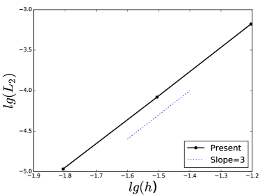
(a) $L_{2}$ in density vs. $h$

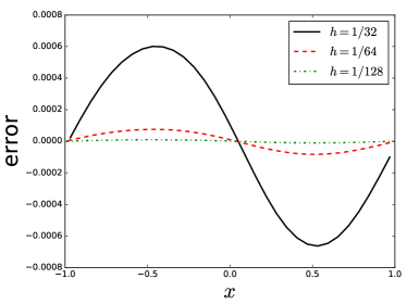
(b) Error distribution with different $h$

Figure 2: The results of accuracy test.

The periodic boundary conditions is implemented at the corresponding bound of the computational domain. The numerical results are shown in Fig.2. It can be concluded that the accuracy designed is achieved in our method, and the error distribution of density shows an excellent performance of the accuracy increase with the mesh resolution.

IV.2 Sod problem

Sod problem is a one-dimensional Riemann problem, which is always used to validate the ability of numerical schemes to capture the discontinuity. The initial condition reads

$$\left(\rho,u,v,p\right)=\left\{\begin{array}[]{ll}\left(1,0,0,1\right),&0<x<0.5,\\ \left(0.125,0,0,0.1\right),&0.5\leq x\leq 1.\end{array}\right.$$ (44)

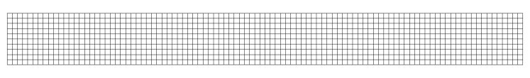
(a) Structured grid

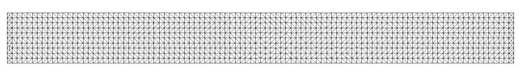
(b) Unstructured grid 1

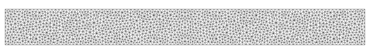
(c) Unstructured grid 2

Figure 3: The grid used in the computation of Sod problem.

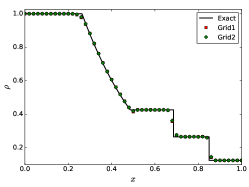
(a) $\rho$

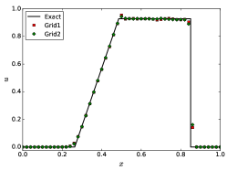
(b) $u$

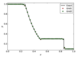
(c) $p$

Figure 4: The numerical results of Sod problem on unstructured grid.

In this case, both the Cartesian grid and unstructured grid are used, and the computational domain is $[0,1]\times[0,0.1]$. The grids used in the computation are shown in Fig. 3, and the length scale $h$ of the grids is $1/100$. The distribution of density, velocity and pressure are shown in Fig. 4. Both the results from two grids have good accordance with the exact solution.

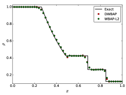
(a) $\rho$

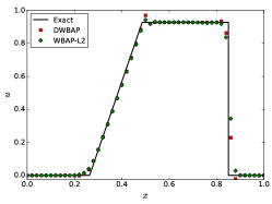
(b) $u$

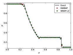
(c) $p$

Figure 5: The effects of limiters in terms of conservative variables on structured grid.

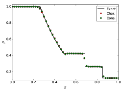
(a) $\rho$

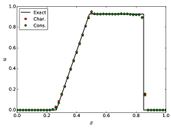
(b) $u$

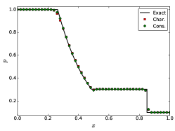
(c) $p$

Figure 6: The behavior of DWBAP limiter in terms of conservative variables and characteristic variables. Char. denotes the characteristic variables. Cons. represents the conservative variables.

The effects of limiters are also investigated. The accuracy of DWBAP limiter has been proved in the reference Liu and Zhang (2017). In this case, we only give some auxiliary notes. The comparison of DWBAP Liu and Zhang (2017) and WBAP-L2 Li and Ren (2012) in terms of conservative variables is shown in Fig. 5, and the results are obtained on a Cartesian grid. In general speaking, DWBAP limiter is a little more accurate than WBAP-L2 limiter. But, for suppressing oscillation, the WBAP-L2 limiter behaviors better. The effects of limiters in terms of conservative and characteristic variables are also considered on unstructured grid in Fig. 3(c). Fig. 6 shows the difference between the DWBAP limiter in terms of conservative variables and characteristic variables respectively. It is obvious that the limiter in terms of characteristic variables has less oscillation. The behavior of high order limiter is a open question, and it is worthy of great efforts. The results above are not the final conclusion, and more investigations are under considered.

IV.3 Lax problem

Lax problem is another one-dimensional Riemann problem. Compared with Sod problem, Lax problem has a more stronger discontinuity. The initial condition is expressed as

$$\left(\rho,u,v,p\right)=\left\{\begin{array}[]{ll}\left(0.445,0.698,0,3.528\right),&0<x<0.5,\\ \left(0.5,0,0,0.571\right),&0.5\leq x\leq 1.\end{array}\right.$$ (45)

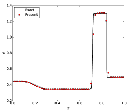
(a) $\rho$

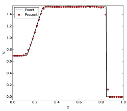
(b) $u$

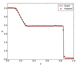
(c) $p$

Figure 7: The numerical results of Lax problem.

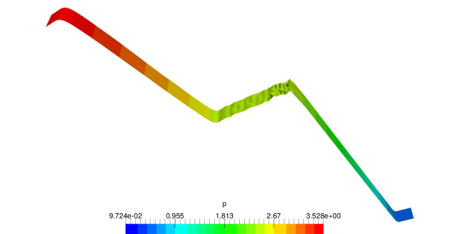
Figure 8: The three-dimensional view of pressure distribution.

The unstructured grid used in the computation is similar to the grid shown in Fig. 3(c), and the length scale $h$ equals to $1/100$. The numerical results are obtained at the time $t=0.14$. Fig. 7 shows the distribution of density, velocity and pressure. The result computed using present method has a good agreement with the exact solution, and the discontinuities are captured accurately. Fig. 8 shows the three-dimensional view of the pressure distribution. Because of the unstructured grid used in the computation, the small oscillation can be seen in the plot. Using the two-dimensional codes to simulate one-dimensional problem on a triangular grid, such a small oscillation is always existed. Not only is in Lax problem, but also in Sod problem and so on.

IV.4 Acoustic pressure pulse

Two-dimensional acoustic pressure pulse problem is a case which the high order method has advantages in resolving the acoustic wave. The initial perturbation is given by a Gaussian pressure distribution at the center of the computational domain at $t=0$.

$$\rho=\rho_{\infty},\quad u=v=0,\quad p=p_{\infty}+\varepsilon e^{-\alpha\eta^{2}},$$ (46)

where $\varepsilon=0.01$, $\eta=\sqrt{(x-0.5)^{2}+(y-0.5)^{2}}$ and $\alpha=\ln{2}/0.04^{2}$. The reference parameters are $p_{ref}=p_{\infty}$, $\rho_{ref}=\rho_{\infty}$, $u_{ref}=\sqrt{p_{ref}/\rho_{ref}}$ and $t_{ref}=l_{ref}/u_{ref}$. The analytical solution Tam and Webb (1993) at time $t$ can be given as

$$p=p_{\infty}+\frac{\epsilon}{2\alpha}\int_{0}^{\infty}e^{-\xi^{2}/(4\alpha)}cos(c_{s}\xi t)J_{0}(\xi\eta)\xi d\xi,$$ (47)

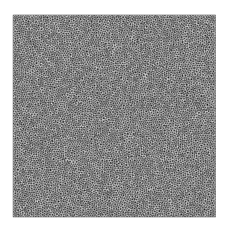
(a) Global view

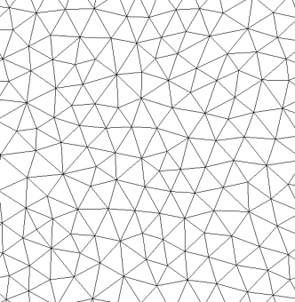
(b) Zoom in view

Figure 9: The unstructured grid ($h=1/80$) used in the simulation of acoustic pressure pulse problem.

where $c_{s}$ represents the sound speed. The computational domain is $[0,1]\times[0,1]$. The unstructured grid used in the computation is exhibited in Fig. 9, and the structured girds used are the Cartesian grids with different length scale $h$.

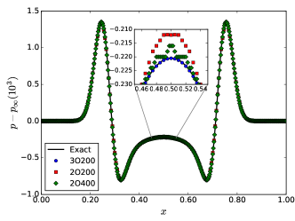
Figure 10: The comparison of the results between second and third order scheme.

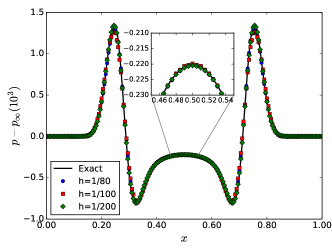
Figure 11: The results of Cartesian grid and triangular gird. The result labeled as $h=1/80$ is computed using triangular gird. The others are simulated on Cartesian grid.

Fig. 10 shows the numerical results of second and third order scheme. The legend ‘xOy’ in picture means the simulation using xth order scheme on a Cartesian grid with $h=1/y$. A conclusion can be drawn that the third order scheme can approach the exact solution more accurate with fewer grid cells. The Fig. 11 exhibits the comparison of results using Cartesian grid and triangular grid, and all the results have good accordance with the analytical solution.

IV.5 Shu-Osher problem

The problem of Shu-Osher Shu and Osher (1988) describes the interaction of an entropy sin wave with a Mach 3 normal shock. The computational domain used in the simulation is taken as $[0,10]\times[0,1]$. The initial condition is given as

$$\left(\rho,u,v,p\right)=\left\{\begin{array}[]{ll}\left(3.857143,2.629369,0.10.33333\right),&0\leq x<1,\\ \left(1+0.2sin(5x),0,0,1\right),&1\leq x\leq 10.\end{array}\right.$$ (48)

The numerical result is obtained at time $t=1.8$. In this case, the Cartesian grid is used, and the length scale $h$ is $1/80$. Because the exact solution of this problem can not be computed directly, the solution of fourth order WENO method with $10000$ grid in one dimension is taken as the exact result. The numerical results are shown in Fig. 12. Compared to the numerical results of second order gas-kinetic scheme and third order WENO Wang and Ren (2015), the advantages of third order method in present work can be seen obviously.

IV.6 Shock-vortex interaction

High order methods have some advantages in the problem of shock-vortex interaction Shu (1998), as it resolves the vortex and the interaction better. In the simulation, a stationary normal shock is initialed in the flow field. A Mach 1.1 normal shock wave is located at the position $x=0.5$. The left side state ($Ma=1.1$) of the shock wave is given as follows

$$(\rho,u,v,p)=(1.0,Ma\sqrt{\gamma},0,1.0),\quad T=p/\rho,\quad S=ln(p/\rho^{\gamma}).$$ (49)

A small and weak vortex is superposed to the left side of the normal shock. The center of the vortex is $(x_{c},y_{c})=(0.25,0.5)$. The perturbation is given as

$$(\delta u,\delta v)=\kappa\eta e^{\mu(1-\eta^{2})}(sin\theta,-cos\theta),$$ (50)

$$\delta T=-\frac{(\gamma-1)\kappa^{2}}{4\mu\gamma}e^{2\mu(1-\eta^{2})}(sin\theta,-cos\theta),\delta S=0,$$ (51)

where

$$\kappa =0.3,$$ (52)

$$\mu =0.204,$$

$$\eta =r/r_{c},$$

$$r_{c} =0.05,$$

$$r =\sqrt{(x-x_{c})^{2}+(y-y_{c})^{2}}.$$

The computational domain and the boundary conditions are shown in Fig. 13. The unstructured grid shown in Fig. 14 is used in this case. The length scale $h$ is $1/80$. The numerical results shown in Fig. 15 are the contours of pressure at different times, and it appears that our present method can capture the shock and the interaction with enough resolution. The picture exhibited in Fig. 16 is the result at time $t=0.8$. It shows clearly that the shock bifurcations reaches to the top boundary, and the reflection is evident.

IV.7 Lid-driven cavity flow

The lid-driven cavity flow is one of the benchmarks for validating the performance of the viscous flow solver. An incompressible flow is initialed in the computational domain, and the Mach number of the lid is set as $Ma=0.1$. The Reynolds number are $Re=400,1000$. The computational domain is $[0,1]\times[0,1]$, and the grid used in this case is the Cartesian grid with $h=1/65$. Fig. 17 and Fig. 18 give numerical results at $Re=400,1000$ respectively, and the results of present work have good accordance with the benchmark data of Ghia Ghia et al. (1982). To reach such a good agreement with the benchmark data, the lower order method should use more grid cells to resolve the flow field compared with present method. It is evident that the numerical method proposed in our paper is also of enough accuracy for viscous flows.

V Conclusion

In present paper, a high order gas-kinetic scheme is proposed based on the CLS reconstruction method. The compacted CLS method used in GKS can achieve third order accuracy on both unstructured and structured grids, which makes CLS method as a very promised algorithm in the field of high order finite volume method. Allied with the third order gas-kinetic flux solver, the third order scheme proposed in our work takes on both the advantages of gas-kinetic scheme and CLS algorithm. The numerical results exhibit that the accuracy designed is approached. Both the results using unstructured grid or structured grid are keeping good accordance with the benchmark data. To suppress oscillations near the discontinuity, two kinds of limiters are investigated in the simulation, and some suggestions are given depended on the numerical results. The effects of limiter in term of conservative variables or characteristic variables are also considered in our work. Compared with the second order gas-kinetic scheme, present method can reach the same level accuracy using fewer grid cells.

References

(a) Stencil for a triangular cell

(b) Stencil for a quadrangular cell

Figure 1: Reconstruction stencil for cell i.

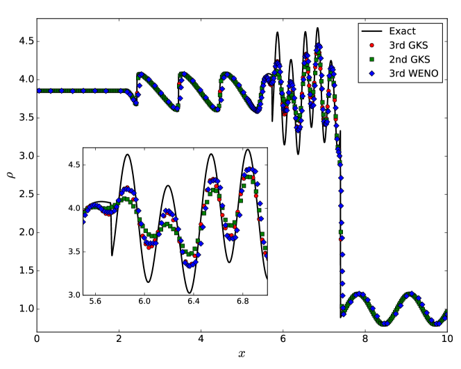
Figure 12: The density distribution of Shu-Osher problem.

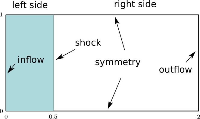
Figure 13: The computational domain and the boundary conditions in the simulation of shock-vortex interaction problem.

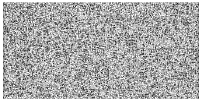
(a) Global view

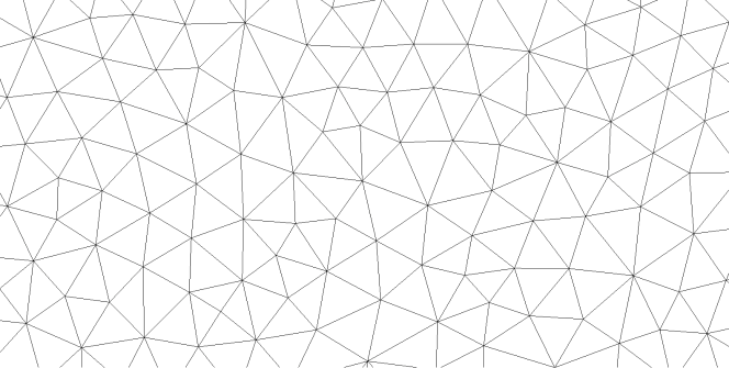
(b) Zoom in view

Figure 14: The unstructured grid used in the simulation of shock-vortex interaction problem.

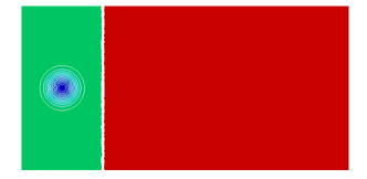
(a) $t=0$

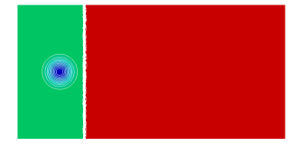
(b) $t=0.05$

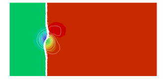
(c) $t=0.2$

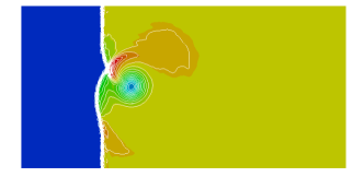
(d) $t=0.35$

Figure 15: The pressure distribution of the shock-vortex interaction problem.

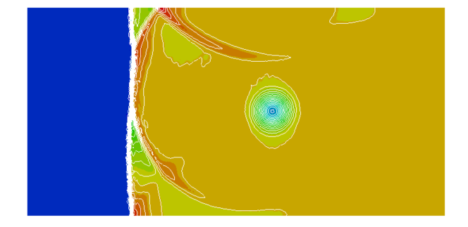
Figure 16: The pressure distribution of the shock-vortex interaction problem at $t=0.8$.

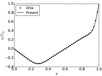
(a) $u$-velocity along the vertical central line.

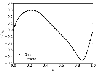
(b) $v$-velocity along the horizontal central line.

Figure 17: The velocity profiles of cavity flow at $Re=400$.

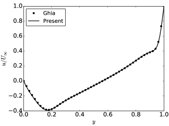
(a) $u$-velocity along the vertical central line.

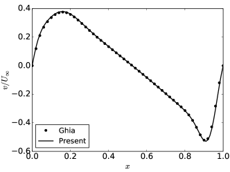
(b) $v$-velocity along the horizontal central line.

Figure 18: The velocity profiles of cavity flow at $Re=1000$.

References

- Liao et al. (2015) F. Liao, Z. Ye, and L. Zhang, Journal of Computational Physics 284, 419 (2015).
- Barth and Frederickson (1990) T. J. Barth and P. O. Frederickson, AIAA paper 90, 0013 (1990).
- Abgrall (1994) R. Abgrall, Journal of Computational Physics 114, 45 (1994).
- Durlofsky et al. (1992) L. J. Durlofsky, B. Engquist, and S. Osher, Journal of Computational Physics 98, 64 (1992).
- Ollivier-Gooch (1997) C. F. Ollivier-Gooch, Journal of Computational Physics 133, 6 (1997).
- Sonar (1997) T. Sonar, Computer Methods in Applied Mechanics and Engineering 140, 157 (1997).
- Liu et al. (1994) X.-D. Liu, S. Osher, and T. Chan, Journal of Computational Physics 115, 200 (1994).
- Shu (1998) C.-W. Shu, in Advanced Numerical Approximation of Nonlinear Hyperbolic Equations (Springer, 1998) pp. 325–432.
- Hu and Shu (1999) C. Hu and C.-W. Shu, Journal of Computational Physics 150, 97 (1999).
- Cockburn and Shu (2001) B. Cockburn and C.-W. Shu, Journal of Scientific Computing 16, 173 (2001).
- Liu et al. (2016) Y. Liu, W. Zhang, Y. Jiang, and Z. Ye, Computers & Mathematics with Applications 72, 1096 (2016).
- Wang (2007) Z. Wang, Progress in Aerospace Sciences 43, 1 (2007).
- Bhatnagar et al. (1954) P. L. Bhatnagar, E. P. Gross, and M. Krook, Physical Review 94, 511 (1954).
- Xu (2001) K. Xu, Journal of Computational Physics 171, 289 (2001).
- Xu et al. (2005) K. Xu, M. Mao, and L. Tang, Journal of Computational Physics 203, 405 (2005).
- Xiong et al. (2011) S. Xiong, C. Zhong, C. Zhuo, K. Li, X. Chen, and J. Cao, International Journal for Numerical Methods in Fluids 67, 1833 (2011).
- Pan et al. (2016a) D. Pan, C. Zhong, J. Li, and C. Zhuo, International Journal for Numerical Methods in Fluids 82, 748 (2016a).
- Li et al. (2016) J. Li, C. Zhong, D. Pan, and C. Zhuo, Computers & Mathematics with Applications (2016), https://doi.org/10.1016/j.camwa.2016.09.012.
- Li et al. (2005) Q. Li, S. Fu, and K. Xu, AIAA Journal 43, 2170 (2005).
- Yuan et al. (2015) R. Yuan, C. Zhong, and H. Zhang, Journal of Computational Physics 296, 184 (2015).
- Yuan and Zhong (2018) R. Yuan and C. Zhong, Applied Mathematical Modelling 55, 417 (2018).
- Li et al. (2014) W. Li, M. Kaneda, and K. Suga, Computers & Fluids 93, 100 (2014).
- Li et al. (2017) J. Li, C. Zhong, Y. Wang, and C. Zhuo, Physical Review E 95, 053307 (2017).
- Li et al. (2010) Q. Li, K. Xu, and S. Fu, Journal of Computational Physics 229, 6715 (2010).
- Luo and Xu (2013) J. Luo and K. Xu, Science China Technological Sciences 56, 2370 (2013).
- Zhou et al. (2017) G. Zhou, K. Xu, and F. Liu, Journal of Computational Physics 339, 146 (2017).
- Pan et al. (2016b) L. Pan, K. Xu, Q. Li, and J. Li, Journal of Computational Physics 326, 197 (2016b).
- Pan and Xu (2015a) L. Pan and K. Xu, Computers & Fluids 119, 250 (2015a).
- Pan and Xu (2015b) L. Pan and K. Xu, Communications in Computational Physics 18, 985 (2015b).
- Pan and Xu (2016) L. Pan and K. Xu, Journal of Computational Physics 318, 327 (2016).
- Wang et al. (2016a) Q. Wang, Y.-X. Ren, and W. Li, Journal of Computational Physics 314, 863 (2016a).
- Wang et al. (2016b) Q. Wang, Y.-X. Ren, and W. Li, Journal of Computational Physics 314, 883 (2016b).
- Saad and Schultz (1986) Y. Saad and M. H. Schultz, SIAM Journal on Scientific and Statistical Computing 7, 856 (1986).
- Saad (2003) Y. Saad, Iterative methods for sparse linear systems (SIAM, 2003).
- Cuthill and McKee (1969) E. Cuthill and J. McKee, in Proceedings of the 1969 24th National Conference (ACM, 1969) pp. 157–172.
- Meijerink and van der Vorst (1981) J. Meijerink and H. van der Vorst, Journal of Computational Physics 44, 134 (1981).
- Hackbusch (1994) W. Hackbusch, Iterative solution of large sparse systems of equations, Vol. 40 (Springer, 1994).
- Liu and Zhang (2017) Y. Liu and W. Zhang, Computers & Fluids 149, 88 (2017).
- Kogan (1969) M. N. Kogan, Rarefied Gas Dynamics (Plenum Press, 1969).
- Gustafsson (1975) B. Gustafsson, Mathematics of Computation 29, 396 (1975).
- Li and Ren (2012) W. Li and Y.-X. Ren, Journal of Computational Physics 231, 4053 (2012).
- Tam and Webb (1993) C. K. Tam and J. C. Webb, Journal of Computational Physics 107, 262 (1993).
- Shu and Osher (1988) C.-W. Shu and S. Osher, Journal of Computational Physics 77, 439 (1988).
- Wang and Ren (2015) Q. Wang and Y.-X. Ren, Journal of Computational Physics 284, 648 (2015).
- Ghia et al. (1982) U. Ghia, K. Ghia, and C. Shin, Journal of Computational Physics 48, 387 (1982).