Hierarchical Aggregation Approach for Distributed clustering of spatial datasets

Abstract

In this paper, we present a new approach of distributed clustering for spatial datasets, based on an innovative and efficient aggregation technique. This distributed approach consists of two phases: 1) local clustering phase, where each node performs a clustering on its local data, 2) aggregation phase, where the local clusters are aggregated to produce global clusters. This approach is characterised by the fact that the local clusters are represented in a simple and efficient way. And The aggregation phase is designed in such a way that the final clusters are compact and accurate while the overall process is efficient in both response time and memory allocation. We evaluated the approach with different datasets and compared it to well-known clustering techniques. The experimental results show that our approach is very promising and outperforms all those algorithms.

I Introduction

Spatio-temporal datasets are often very large and difficult to analyse  [1]. Traditional centralised data management and mining techniques are not adequate, as they do not consider all the issues of data-driven applications such as scalability in both response time and accuracy of solutions, distribution and heterogeneity  [2]. In addition, transferring a huge amount of data over the network is not an efficient strategy and may not be possible for security and protection reasons.

Distributed data mining (DDM) techniques constitute a better alternative as they are scalable and can deal efficiently with data heterogeneity. Many DDM methods such as distributed association rules and distributed classification have been proposed in the last decade and most of them are based on performing partial analysis on local data at individual sites followed by the generation of global models by aggregating those local results [3, 4, 5, 6]. However, only a few of them concern distributed clustering. Among these many parallel clustering algorithms have been proposed  [7, 8, 9]. They are classified into two categories. The first consists of methods requiring multiple rounds of message passing and significant amount of synchronisations. The second category consists of methods that build local clustering models and then aggregate them to build global models  [10]. Most of the parallel approaches need either multiple synchronisation constraints between processes or a global view of the dataset, or both  [11, 12]. For distributed approaches, the aggregation phase is very costly, and therefore, it needs to be optimised.

In this paper, we present an approach that reduces the complexity of the aggregation phase. It reduces significantly the amount of information exchanged during the aggregation phase, and generates automatically the correct number of clusters. In a case study, it was shown that the data exchanged is reduced by more than $98\%$ of the original datasets.

II Dynamic Distributed Clustering

The DDC approach includes two main steps. In the first step, as usual, we cluster the datasets located on each node and select good local representatives for each local cluster. This phase is executed in parallel without communications between the nodes. In this phase we can reach a super speed-up. The next phase consists of aggregating the local clusters. This operation is executed by certain nodes of the system, called leaders. The leaders are elected according to some nodes’ characteristics such as their capacity, processing power, connectivity, etc. The leaders are responsible for merging and regenerating the data objects based on the local cluster representatives. However, the nodes need to communicate in order to send their local clusters to the leaders. This process is shown in Figure 1.

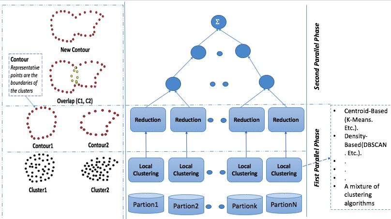
Figure 1: An overview of the DDC Approach.

II-A Local Models

Each node can use any technique of clustering on its local dataset. This is one of the key features of this approach to deal with data heterogeneity. Each node choses a technique that is more suitable for its data. This approach relaxes the data pre-processing. For instance we may not need to deal with data consistency between the nodes’ datasets. All needed is the consistency of the local cluster’s representation. Once extracted the local clusters will be used as inputs for the next phase to generate global clusters. However exchanging the local clusters through the network will create significant overheads and slowdown hugely the process. This is one of the major problems of the majority of distributed clustering techniques. To improve the performance we propose to exchange a minimum number of points/objects. Instead of sending all the clusters datapoints, we only exchange their representative points, which constitute $1\%$ to $2\%$ of the total size of the dataset.

The best way to represent a spatial cluster is by its shape and density. The shape of a cluster is represented by its boundary points (called contour)  [11, 13, 14] (see Figure 4). Many algorithms for extracting the boundaries from a cluster can be found in the literature  [15, 16]. Recently, we developed a new algorithm for detecting and extracting the boundary of a cluster  [10]. The main concepts of this technique are given below.

Neighbourhood:  Given a cluster $C\subseteq\Re^{n}\equiv\{p_{1},p_{2},...,p_{n}\}$ The neighbourhood $N^{C}(p)$ of a point $p$ in the cluster $C$ is defined as the set of points ${p_{i}}\in C$ so that the distance between $p_{i}$ and $p$ is less than or equal to $\varepsilon$:

$$N^{C}(p)=\{p_{i}\in C\mid dist(p,p_{i})\leq\varepsilon\}$$ (1)

In order to determine the boundary points of a cluster, we need to introduce the following concepts:

Displacement vector:  A displacement vector from $p_{i}\in N^{C}(p)$ to the point $p$ is defined as:

$$\overrightarrow{\rm V}=\sum_{p_{i}\in N^{C}(p)}(p-p_{i})$$ (2)

This vector points towards the area of the lowest density of the neighbourhood of $p$.

Balance vector:  The balance vector relative to the point $p$ is defined as follows:

$$\overrightarrow{\rm b}_{p}=\begin{cases}\frac{1}{\|\overrightarrow{\rm V}_{p}\|}\overrightarrow{\rm V}_{p}&\mbox{\leavevmode\nobreak\ if\leavevmode\nobreak\ }{\|\overrightarrow{\rm V}_{p}\|}>0\\ \overrightarrow{\rm 0}&\mbox{Otherwise}\end{cases}$$ (3)

Note that the balance vector of $p$ points to the least dense area of the neighbourhood of $p$, the length of the vector does not hold any relevant information. Figure 2 shows an example of a balance vector. The neighbourhoods of $p$ are inside the circle, the balance vector is represented by the blue colour.

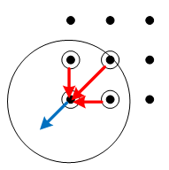
Figure 2: Example of a balance vector.

Boundary points:  If a point is a boundary point, there should be no points towards the direction of the balance vector. This property allows us to separate boundary points and internal points. For each point $p$, it checks for an empty area whose shape is the intersection of an hyper-cone of infinite height, vertex, axis and aperture $\rho$, where $\rho$ is a given angle. As shown in 3, the area checked is highlighted in green. Formally, a boundary point is described as a Boolean predicate.

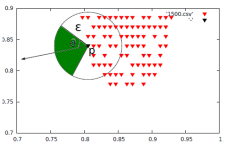
Figure 3: Boundary point check

$$\small Boundary(p)=\begin{cases}true&\mbox{\leavevmode\nobreak\ if\leavevmode\nobreak\ }(\forall q\in N_{\varepsilon}^{C}(p),(q-p)\overrightarrow{\rm b}_{b}<\cos(v)\\ false&\mbox{Otherwise}\end{cases}$$ (4)

We can define the boundary $B_{C}$ of a cluster $C$ as the set of all boundary points in $C$:

$$B_{C}=\{p\in C:\mbox{Boundary(p) is true}\}$$ (5)

The algorithm for selecting the boundary points is described in Algorithm 1, and its complexity is $\mathcal{O}(n\log{n})$.

input : Cluster $C$, set of balance vectors ${\overrightarrow{\rm b}_{p_{i}}}$, parameter $\nu$.

output : Boundary points $B_{C}$ of cluster $C$

1

2$B_{C}\leftarrow C$;

3 for every point $p\in B_{C}$ do

4       for every point $q\in N^{C}(p)$ do

5             if $(q-p)\overrightarrow{\rm b}\geq\cos(v)$ then

6                   Discard $p$ from $B_{C}$;

7                   Break;

8                  

9            

10      

11return $B_{C}$;

Algorithm 1 Boundary Detection Algorithm

Let $C_{i}$ be a set of clusters of node $i$ and $B_{c_{j}}$ be the boundary of a cluster $c_{j}\in C_{i}$. The local model $L_{i}$ is defined by:

$$L_{i}={\bigcup_{j=1}^{n}{B_{c_{j}}}\cup P_{i}}$$ (6)

Where $P_{i}$ is the set of internal representatives.

II-B Global Models

The global clusters are generated during the second phase. This phase consists of two main steps: 1) each leader collects the local clusters of its neighbours, 2) the leaders merge the local clusters using the overlay technique. The process of merging clusters will continue until we reach the root node. The root node will contain the global clusters (see Figure 1). During this phase we only exchange the boundaries of the clusters.

The merging process consists of two steps: boundary merging and regeneration. The merging is performed by a boundary-based method. Let $L_{i}$ be a local model received from the site $i$ and $B_{i}$ be the set of all boundaries in $L_{i}$. The global model $G$ is defined by:

$$G={\Gamma(\cup B_{i}),B_{i}\in L_{i}}$$ (7)

where $\Gamma$ is a merging function.

III DDC Evaluation and Validation

DDC is evaluated using different clustering algorithms. In this paper we use a centroid-based algorithm (K-Means) and a density-based Algorithm (DBSCAN).

III-A DDC-K-Means

The DDC with K-Means (DDC-K-Means) is characterised by the fact that in the first phase, called the parallel phase, each node $N_{i}$ of the system executes the K-Means algorithm on its local dataset to produce $L_{i}$ local clusters and calculate their contours. The rest of the process is the same as described above. It was shown in [17] that DDC-K-Means dynamically determines the number of the clusters without a priori knowledge about the data or an estimation process of the number of the clusters. DDC-K-Means was compared to two well-known clustering algorithms: BIRCH  [18] and CURE  [19]. The results showed that it generates much better clusters. Also, as expected, this approach runs much faster than the two other algorithms; BIRCH and CURE.

DDC-K-Means does not need the number of global clusters in advance. It is calculated dynamically. Moreover, each local clustering $L_{i}$ needs $K_{i}$. Let $\tilde{K_{i}}$ be the exact number of local clusters in the node $N_{i}$, all it is required is to set $K_{i}$ such that $K_{i}>\tilde{K_{i}}$. This is much simpler than giving $K_{i}$, especially when there is not enough knowledge about the local dataset characteristics. Nevertheless, it is indeed better to set $K_{i}$ as close as possible to $\tilde{K_{i}}$ in order to reduce the processing time in calculating the contours and also merging procedure.

However, DDC-K-Means fails to find good clusters for datasets with Non-Covex shapes and also for datasets with noises, this is due to the fact that the K-Means algorithm tends to work with convex shape only, because it is based on the centroid principle to generate clusters. Moreover, we can also notice that the results of DDC-K-Means are even worse with dataset which contains a big amount of noises ($T_{3}$, and $T_{4}$). In fact it returns the whole dataset with the noise as one final cluster for each dataset (see Figure 5). This is because K-Means does not deal with noise.

III-B DDC with DBSCAN

DBSCAN (Density-Based spatial Clustering of Applications with Noise) is a well-known density based clustering algorithm capable of discovering clusters with arbitrary shapes and eliminating noisy data  [20].

III-B1 DBSCAN Complexity

DBSCAN visits each point of the dataset, possibly multiple times, depending on the size of the neighbourhood. If it performs a neighbourhood operations in $\mathcal{O}(\log n)$, an overall average complexity of $\mathcal{O}(n\log n)$ is obtained if the parameter $Eps$ is chosen in a meaningful way. The worst case execution time complexity remains $\mathcal{O}(n^{2})$. The distance matrix of size $\mathcal{O}((n^{2}-n/2))$ can be materialised to avoid distance re-computations, but this needs $\mathcal{O}(n^{2})$ of memory, whereas a non-matrix based implementation of DBSCAN only needs $O(n)$ of memory space.

III-B2 DDC-DBSCAN Algorithm

The approach remains the same; instead of using K-Means for processing local clusters, we use DBSCAN. Each node ($n_{i}$) executes DBSCAN on its local dataset to produce $K_{i}$ local clusters. Once all the local clusters are determined, we calculate their contours. The second phase is the same and the pseudo code of the algorithm is given in Algorithm 2.

input : $X_{i}$: Dataset Fragment, $Eps_{i}$: Distance $Eps_{i}$ for $Node_{i}$, $MinPts_{i}$: minimum points contain clusters generated by $Node_{i}$, $D$: tree degree, $L_{i}$: Local clusters generated by $Node_{i}$

output : $K_{g}$: Global Clusters (global results)

1 $level=treeheight$;

2

1. DBSCAN($X_{i}$. $Eps_{i}$, $MinPts_{i}$);

// $Node_{i}$ executes DBSCAN locally.

Contour($L_{i}$);

// $Node_{i}$ executes the Contour algorithm to generate the boundary of each local cluster.

$Node_{i}$ joins a group $G$ of $D$ elements;

// $Node_{i}$ joins its neighbourhood

Compare cluster of $Node_{i}$ to other node’s clusters in the same group;

// look for overlapping between clusters.

j = ElectLeaderNode();

8 // Elect a node which will merge the overlapping clusters. if $i<>j$ then

9       Send (contour i, j);

10      

11else

12       if $level>0$ then

13             $level$ - - ;

14             Repeat 3, 4, and 5 until level=0;

15            

16      else

17             return ($K_{g}$: $Node_{i}$’ clusters);

18            

19      

Algorithm 2 DDC with DBSCAN.

Figure 4 illustrates an example of DDC-DBSCAN. Assume that the distributed computing platform contains five Nodes ($N=5$). Each Node executes DBSCAN algorithm with its local parameters ($Eps_{i}$, $MinPts_{i}$) on its local dataset. As it can be seen in Figure 4 the new approach returned exactly the right number of clusters and their shapes. The approach is insensitive to the way the original data was distributed among the nodes. It is also insensitive to noise and outliers. As we can see, although each node executed DBSCAN locally with different parameters. The global final clusters were correct even on the noisy dataset ($T_{3}$) (See Figure 4).

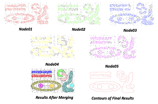
Figure 4: Example of DDC-DBSCAN execution.

IV Experimental Results

In this section, we study the performance of the DDC-DBSCAN approach and demonstrate its effectiveness compared to BIRCH, CURE and DDC-K-Means. We choose these algorithms because either they are in the same category such as BIRCH which belongs to hierarchical clustering category, or have an efficient optimisation approach, such as CURE.

BIRCH: We used the BIRCH implementation provided in [18]. It performs a pre-clustering and then uses a centroid-based hierarchical clustering algorithm. Note that the time and space complexity of this approach is quadratic to the number of points after pre-clustering. We set its parameters to the default values as suggested in [18].

CURE: We used the implementation of CURE provided in [19]. The algorithm uses representative points with shrinking towards the mean. As described in [19], when two clusters are merged in each step of the algorithm, representative points for the new merged cluster are selected from the ones of the two original clusters rather than all the points in the merged clusters.

IV-A Experiments

We run experiments with different datasets. We used four types of datasets ($T_{1}$, $T_{2}$, $T_{3}$ and $T_{4}$) with different shapes and sizes. These datasets are very well-known benchmarks to evaluate density-based clustering algorithms. All the four datasets are summarised in Table I. The number of points and clusters in each dataset is also given. These four datasets contain a set of shapes or patterns which are not easy to extract with traditional techniques.

Table I: The datasets used to test the algorithms.

Type	Dataset	Description	#Points	#Clusters
Without Noise	T1	Round and Oval shape	700	5
With Noise	T2	Different shapes including noise	321	6
	T3	Different shapes, with some clusters surrounded by others	10,000	9
	T4	Different shapes with Noises	8,000	6

IV-B Quality of Clustering

We run the four algorithms on the Four datasets in order to evaluate the quality of their final clusters. Figure 5 shows the clusters returned by each of the four algorithms for the datasets without noise ($T_{1}$) and datasets with noise ($T_{2},T_{3},$ and $T_{4}$). We use different colours to show the clusters returned by each algorithm.

BIRCH	CURE	DDC-K-Means	DDC-DBSCAN
T1
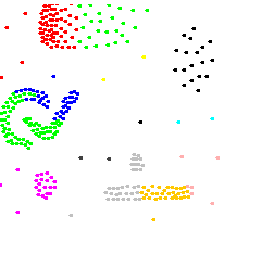
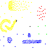
T2
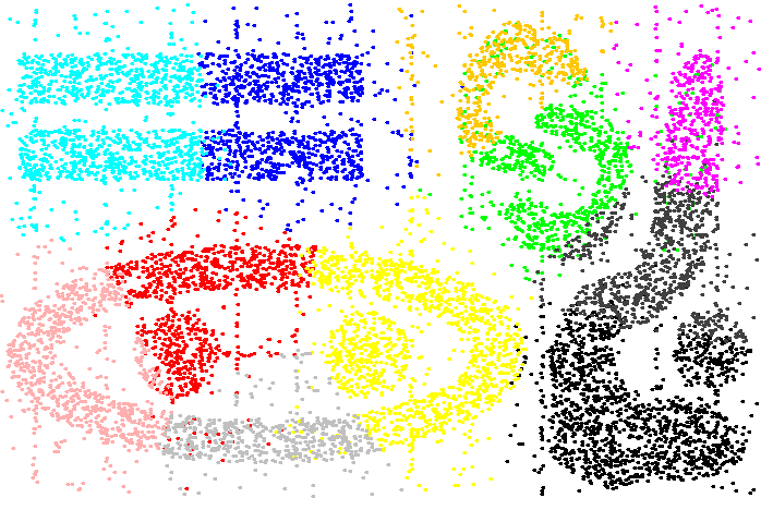
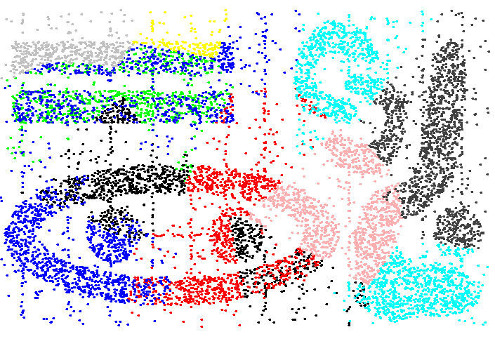
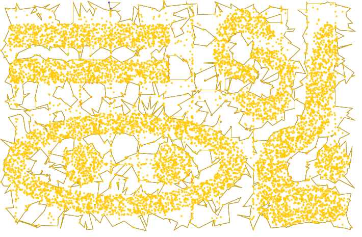
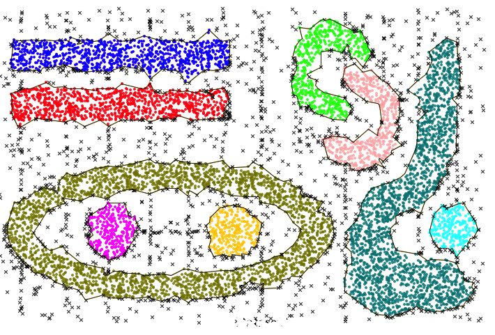
T3
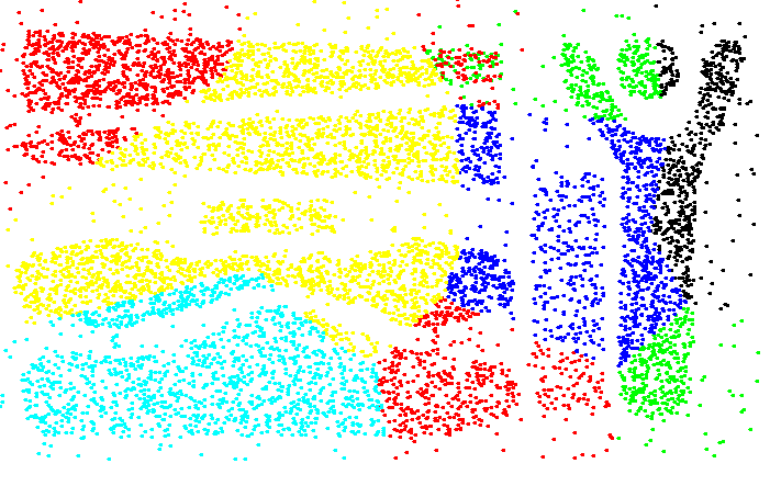
T4

Figure 5: Comparing the clusters generated across different datasets

As expected, BIRCH could not find correct clusters; it tends to work slightly better with datasets without noise ($T_{1}$), as BIRCH does not deal with noise. The results of CURE are worse and it is not able to extract clusters with non-convex shapes. We can also see that CURE does not deal with noise. DDC-K-Means fails to find the correct final results. In fact it returns the whole original dataset as one final cluster for each dataset ($T_{3}$ and $T_{4}$) (Which contain significant amount of noise). This confirms that the DDC technique is sensitive to the type of the algorithm chosen for the first phase. Because the second phase deals only with the merging of the local clusters whether they are correct or not. This issue is corrected by the DDC-DBSCAN, as it is well suited for spatial datasets with or without noise. For datasets with noise it eliminates the noise and outliers. In fact, it generates good final clusters in datasets that have significant amount of noise.

As a final observation, these results prove that the DDC framework is very efficient with regard to the accuracy of its results. The only issue is to choose a good clustering algorithm for the first phase. This can be done by exploring the initial datasets along with the question to be answered and choose an appropriate clustering algorithm accordingly.

Moreover, as for the DDC-K-Means, DDC-DBSCAN is dynamic (the correct number of clusters is returned automatically) and efficient (the approach is distributed and minimises the communications).

IV-C Speed-up

The goal here is to study the execution time of the four algorithms and demonstrate the impact of using a parallel and distributed architecture to deal with the limited capacity of a centralised system.

As mentioned in Section III-B1, the execution time for the DDC-DBSCAN algorithm can be generated in two cases. The first case is to include the time required to generate the distance matrix calculation. The second case is to suppose that the distance matrix has already been generated. The reason for this is that the distance matrix is calculated only once.

Table II: The execution times (ms) of BIRCH, CURE, DDC-K-Means and DDC-DBSCAN with (w) and without (w/o) distance matrix computation.

		Execution Time (ms)
					DDC-DBSCAN
	SIZE	BIRCH	CURE	DDC-K-Means	W	W/O
T1	700	150	70045	120	500	302
T2	321	72	47045	143	504	312
T3	10000	250	141864	270	836	470
T4	8000	218	92440	257	608	304

Table II illustrates the execution times of the four techniques on different datasets. Note that the execution times do not include the time for post-processing since these are the same for the four algorithms.

As mentioned in Section III-B1, Table II confirmed the fact that the distance matrix calculation in DBSCAN is very significant. Moreover, DDC-DBSCAN’s execution time is much lower than CURE’s execution times across the four datasets. Table II shows also that the DDC-K-Means is very quick which is in line with its polynomial computational complexity. BIRCH is also very fast, however, the quality of its results are not good, it failed in finding the correct clusters across all the four datasets.

The DDC-DBSCAN is a bit slower that DDC-K-Means, but it returns high quality results for all the tested benchmarks, much better that DDC-K-Means, which has reasonably good results for convex cluster shapes and very bad results for non-convex cluster shapes. The overall results confirm that the DDC-DBSCAN clustering techniques compares favourably to all the tested algorithms for the combined performance measures (quality of the results and response time).

IV-D Computation Complexity

Let $n$ be the number of data objects in the dataset. The complexity of our approach is the sum of the complexities of its three components: local mining, local reduction, and global aggregation.

Phase1: Local clustering

Assume that the local clustering algorithm is DBSCAN for all the nodes. The cost of this phase is given by:

$$T_{Phase_{1}}=\operatorname*{Max}_{i=1}^{N}(DBSCAN_{i})+\operatorname*{Max}_{i=1}^{N}(Reduction_{i})$$

Where $N$ is the number of nodes in the system. The complexity of DBSCAN in the best case scenario is $\mathcal{O}(n\log n)$ if the parameter $Eps$ is chosen in a meaningful way and also if we exclude the distance matrix computation. Finally, the complexity of the local reduction algorithm is $\mathcal{O}(n\log{}n)$.

Phase2: Aggregation

Our global aggregation depends on the hierarchical combination of contours of local clusters. As the combination is based on the intersection of edges from the contours, the complexity of this phase is $\mathcal{O}(v\log{}v+p)$. Where $v$ is the number of vertices and $p$ is the number of intersections between edges of different contours (polygons).

Total complexity

The total complexity of our approach is $T_{Total}=\mathcal{O}(n\log n)+\mathcal{O}(n\log{}n)+\mathcal{O}(v\log{}v+p)$, which is:

$$T_{Total}\simeq\mathcal{O}(n\log n)$$

V Conclusion

In this paper, we proposed an efficient and flexible distributed clustering framework that can work with existing data mining algorithms. The framework has been tested on spatial datasets using the K-Means and DBSCAN algorithms. The proposed approach is dynamic, which solves one of the major shortcomings of K-Means or DBSCAN. We proposed an efficient aggregation phase, which reduces considerably the data exchange between the leaders and the system nodes. The size of the data exchange is reduced by about $98\%$.

The DDC approach was tested using various benchmarks. The benchmarks were chosen in such a way to reflect all the difficulties of clusters extraction. These difficulties include the shapes of the clusters (convex and non-convex), the data volume, and the computational complexity. Experimental results showed that the approach is very efficient and can deal with various situations (various shapes, densities, size, etc.).

As future work, we will try to extend the framework to non-spatial datasets. We will also look at the problem of the data and communications reduction during phase two.

John Doe

References

- [1] M. H. Dunham and D. Ming, “Introductory and advanced topics,” 2003.
- [2] M. Bertolotto, S. Di Martino, F. Ferrucci, and M.-T. Kechadi, “Towards a framework for mining and analysing spatio-temporal datasets,” International Journal of Geographical Information Science, vol. 21, no. 8, pp. 895–906, 2007.
- [3] L. Aouad, N.-A. Le-Khac, and M.-T. Kechadi, “weight clustering technique for distributed data mining applications,” LNCS on advances in data mining – theoretical aspects and applications, vol. 4597, pp. 120–134, 2007.
- [4] L.Aouad, N.-A. Le-Khac, and M.-T. Kechadi, “Grid-based approaches for distributed data mining applications,” Journal of Algorithms & Computational Technology, vol. 3, no. 4, pp. 517–534, 2009.
- [5] N.-A. Le-Khac, L. Aouad, and M.-T. Kechadi, “Performance study of distributed apriori-like frequent itemsets mining,” Knowledge and Information Systems, vol. 23, no. 1, pp. 55–72, 2010.
- [6] N. Le-Khac, L.Aouad., and M.-T. Kechadi, Emergent Web Intelligence: Advanced Semantic Technologies. Springer London, 2010, ch. Toward Distributed Knowledge Discovery on Grid Systems, pp. 213–243.
- [7] L. Aouad, N.-A. Le-Khac, and M.-T. Kechadi., “Image analysis platform for data management in the meteorological domain,” in 7th Industrial Conference, ICDM 2007, Leipzig, Germany, July 14-18, 2007. Proceedings, vol. 4597. Springer Berlin Heidelberg, 2007, pp. 120–134.
- [8] I. Dhillon and D. Modha, “A data-clustering algorithm on distributed memory multiprocessor,” in large-Scale Parallel Data Mining, Workshop on Large-Scale Parallel KDD Systems, SIGKDD. Springer-Verlag London, UK, 1999, pp. 245–260.
- [9] M. Ester, H.-P. Kriegel, J. Sander, and X. Xu, “A density-based algorithm for discovering clusters in large spatial databases with noise.” in Kdd, vol. 96, no. 34, 1996, pp. 226–231.
- [10] J.-F. Laloux, N.-A. Le-Khac, and M.-T. Kechadi, “Efficient distributed approach for density-based clustering,” Enabling Technologies: Infrastructure for Collaborative Enterprises (WETICE), 20th IEEE International Workshops, pp. 145–150, 2011.
- [11] N. Le-Khac, L.Aouad., and M.-T. Kechadi, Data Management. Data, Data Everywhere: 24th British National Conference on Databases. Springer Berlin Heidelberg, 2007, ch. A New Approach for Distributed Density Based Clustering on Grid Platform, pp. 247–258.
- [12] L. Aouad, N.-A. L. Khac, and M.-T. Kechadi, Advances in Data Mining. Theoretical Aspects and Applications: 7th Industrial Conference (ICDM 2007), Leipzig, Germany, July 14-18, 2007. Proceedings. Springer Berlin Heidelberg, 2007, ch. Lightweight Clustering Technique for Distributed Data Mining Applications, pp. 120–134.
- [13] L.Aouad, N.-A. Le-Khac, and M-T.Kechadi, “Variance-based clustering technique for distributed data mining applications.” in DMIN, 2007, pp. 111–117.
- [14] N.-A. Le-Khac, M. Bue, M. Whelan, and M-T.Kechadi, “A knowledge based data reduction for very large spatio-temporal datasets,” International Conference on Advanced Data Mining and Applications, (ADMA’2010), 2010.
- [15] A. Chaudhuri, B. Chaudhuri, and S. Parui, “A novel approach to computation of the shape of a dot pattern and extraction of its perceptual border,” Computer vision and Image Understranding, vol. 68, pp. 257–275, 1997.
- [16] M. Melkemi and M. Djebali, “Computing the shape of a planar points set,” Elsevier Science, vol. 33, p. 1423–1436, 2000.
- [17] M. Bendechache and M.-T. Kechadi, “Distributed clustering algorithm for spatial data mining,” in Spatial Data Mining and Geographical Knowledge Services (ICSDM), 2015 2nd IEEE International Conference on, 2015, pp. 60–65.
- [18] T. Zhang, R. Ramakrishnan, and M. Livny, “Birch: An efficient data clustering method for very large databases,” in SIGMOD-96 Proceedings of the 1996 ACM SIGMOD international conference on Management of data, vol. 25. ACM New York, USA, 1996, pp. 103–114.
- [19] S. Guha, R. Rastogi, and K. Shim, “Cure: An efficient clustering algorithm for large databases,” in Information Systems, vol. 26. Elsevier Science Ltd. Oxford, UK, 2001, pp. 35–58.
- [20] M.Ester, H. Kriegel, J. Sander, and X. Xu, “A density-based algorithm for discovering clusters in large spatial databases with noise,” In 2nd Int. Conf., Knowledge Discovery and Data Mining (KDD 96), 1996.