Disentangling Respiratory Sinus Arrhythmia in Heart Rate Variability Records

Abstract

Different measures of heart rate variability and particularly of respiratory sinus arrhythmia are widely used in research and clinical applications. Inspired by the ideas from the theory of coupled oscillators, we use simultaneous measurements of respiratory and cardiac activity to perform a nonlinear decomposition of the heart rate variability into the respiratory-related component and the rest. We suggest to exploit the technique as a universal preprocessing tool, both for the analysis of respiratory influence on the heart rate as well as in cases when effects of other factors on the heart rate variability are in focus. The theoretical consideration is illustrated by the analysis of 25 data sets from healthy subjects.

I Introduction

Heart rate variability (HRV) is a non-invasive measure of autonomic nervous system function. Therefore, its analysis and quantification are increasingly used in physiological and medical research as well as in clinical practice. Typically, HRV denotes variation of the inter-beat intervals, in most cases defined as the intervals between the well-pronounced R-peaks in an electrocardiogram (ECG), and therefore called RR-intervals. A particularly important component of HRV is a modulation of the RR-intervals by respiratory influence, called respiratory sinus arrhythmia (RSA) Katona-Jih-75 ; Hirsch-Bishop-81 ; Hayano842 ; Billman-11 ; Moser1994 . Physiological significance of RSA is, on one hand, in facilitating gas exchange between the lungs and the blood and thus helping the heart to do less work while maintaining optimal levels of blood gases Larsen_et_al-10 ; TJP:TJP4976 . On the other hand, biological advantage of RSA is the stabilization of blood flow to the brain and the periphery by compensating arterial pressure changes arising from intrathoracic pressure changes due to in- and expiration. It has been shown that blood pressure oscillations, connected to respiration, are reduced and, therefore, the blood flow is stabilized by RSA Elstad2014 . In medicine, the amplitude or the spectral power of RSA is used as a smart noninvasive measure for vagal tone Moser1994 . The reason for this dominantly vagal origin of RSA can be found in the vagal synapses, which are faster than the sympathetic ones and are therefore able to translate central respiratory oscillations present in the brainstem to changes of cardiac sinus node discharge rate, which is not the case for slow sympathetic synapses Moser2017 .

Vagal tone is gaining importance in preventive and aging medicine as the tone decreases with age Baylis2013 ; Lehofer1999 and also because of chronic diseases Lehofer1997 ; Das2001 . This understanding got momentum, when a vagal inflammatory reflex was discovered Tracey2002 , indicating a close inverse connection between the available vagal tone and silent inflammation, a condition obviously resulting in chronic diseases like vascular sclerosis, Alzheimer disease, and even cancer (see Nathan2002 for a comprehensive overview). Since the accuracy of vagal tone determination by common time or frequency domain methods of RSA quantification, especially under conditions of different respiratory patterns, have been questioned Laborde2017 , it is highly important to improve the methods for separation of respiratory and other influences of the autonomic nervous system on HRV.

A variety of data analysis techniques quantifying RSA have been proposed in the literature; for a discussion of commonly used metrics and their advantages and drawbacks see, e.g., Lewis_et_al-12 . Examples of application of RSA analysis include clinical psychology Wielgus-Aldrich-Mezulis-Crowell-16 , treatment of substance use disorder Price-Crowell-16 , prediction of the course of depression Panaite_et_al-16 , quantification of cardiac vagal tone and its relation to evolutionary and behavioral functions Grossman-Taylor-07 , quantification of vagal activity during stress in infants Ritz_et_al-12 and even in cancer patients Moser2006 , to name just a few. On the other hand, quantification of the HRV component, not related to respiration, is important for the analysis of long-range and scaling properties of the cardiac dynamics Ivanov_et_al_99a ; Schmitt-Ivanov-07 .

In this paper we, following our previous study Kralemann_et_al-13 , elaborate on a nonlinear technique that allows us to decompose the HRV into a respiratory-related component (R-HRV), and a component where variability is caused by all other sources; we denote the latter component as NR-HRV. After the decomposition, both components can be subject to any existing analysis techniques. Thus, the suggested disentanglement can serve as a universal preprocessing tool that allows a researcher to concentrate on particular aspects of HRV: if the interest is in a respiratory caused modulation of the heart rate, then it makes sense to work with the R-HRV component. On the contrary, if the variation of the heart rhythm in a different frequency range is important, then it makes sense to first cleanse the data from the respiratory caused variability, and then to analyze NR-HRV.

Separation of respiratory influences from HRV records was also treated before by different ad hoc techniques Widjaja_et_al-14 ; Kuo-Kuo-16 like adaptive filtering, least-mean-error fitting of power spectra, and principal component analysis. Our approach is based on the idea from nonlinear dynamics and coupled oscillators theory Winfree-80 ; Glass-01 ; Pikovsky-Rosenblum-Kurths-01 ; Strogatz-03 . Within this framework, we treat cardio-vascular and respiratory systems as two interacting endogenous, self-sustained, oscillators, what allows for a low-dimensional description of their dynamics in terms of phases. This description, in its turn, provides the desired disentanglement and better quantification of the corresponding HRV components, as described below.

II Methods

II.1 Theoretical Background

We start with a general theory, briefly presenting a phase-based description of the dynamics of interacting oscillators. In the simplest case of an autonomous noisy periodic or weakly chaotic oscillator the phase dynamics obeys

$$\dot{\varphi}=\omega+\zeta(t)\;,$$ (1)

where $\varphi$ and $\omega$ are the phase and the natural frequency of the system, and the noise term $\zeta(t)$ accounts for intrinsic fluctuations of the system parameters. If the system experiences external influences from different sources (which may be either regular or not), then, according to the dynamical perturbation theory (see, e.g., Pikovsky-Rosenblum-Kurths-01 for details), the leading effect of the external forces $\eta_{s}(t)$, where $s=1,2,\ldots$, is in the modulation of the phase, which now obeys

$$\dot{\varphi}=\omega+\sum_{s}q_{s}[\varphi,\eta_{s}(t)]+\zeta(t)\;.$$ (2)

Here $q_{s}$ are coupling functions describing response to the corresponding perturbations. It accounts for the property that susceptibility of an oscillator to external perturbations generally depends on its phase. Notice that the forces $\eta_{s}(t)$ can have arbitrary complex time dependence, i.e. they can be periodic, chaotic, or stochastic.

Suppose now that one of the forces, say the first one, $\eta_{1}(t)$, and the corresponding coupling function $q_{1}$, are known. Then we can use Eq. (2) in order to represent the variations of the instantaneous frequency as a sum of two components,

$$\dot{\varphi}=\omega+q_{1}(\varphi,\eta_{1}(t))+\xi(\varphi,t)\;,$$ (3)

where $q_{1}(\varphi,\eta_{1}(t))$ describes solely the impact of the force $\eta_{1}(t)$ on the phase dynamics, while

$$\xi(\varphi,t)=\sum_{s\neq 1}q_{s}(\varphi,\eta_{s}(t))+\zeta(t)$$ (4)

describes a cumulative effect of all other forces and of the intrinsic fluctuations. The representation by Eq. (3) plays the central role in our approach.

Now we specify the theory to cover the system of our interest, namely the cardiovascular system. In particular, we consider the experiments where both cardiac and respiratory activities are monitored simultaneously, and the ECG and the respiratory signal, e.g. the air flow at the nose, are registered. It is natural to represent these two endogenous rhythms as outputs of two interacting oscillatory systems, which can be characterized by their phases. As discussed in details below, these phases can be estimated from data.

Denoting the phase and the natural frequency of the cardiac oscillator with $\varphi$ and $\omega$, respectively, we write, similarly to (3):

$$\dot{\varphi}=\omega+q_{r}(\varphi,\eta_{r}(t))+\xi(\varphi,t)\;,$$ (5)

where the subscript $r$ stands for respiration, and $\eta_{r}$ describes effect of the respiration on the cardiac frequency. The term $\xi(\varphi,t)$, like in Eq. (4), describes the effect on the cardiac phase of the physiological rhythms other than respiration, as well as of non-rhythmical, stochastic, external and intrinsic perturbations.

In practice, measurements of respiration rather often (and in our experiments as well) do not provide a proper magnitude of the corresponding force $\eta_{r}$, but only its phase $\psi(t)$. Thus, we assume that the forcing term due to respiration is a $2\pi$-periodic function of the time-dependent respiratory phase $\psi$. So, we write $\eta_{r}(t)=S(\psi(t))=S(\psi(t)+2\pi)$, and replace the coupling function $q_{r}(\varphi,\eta_{r}(t))$ in Eq. (5) by a phase-based coupling function $Q(\varphi,\psi)$, obtaining thus

$$\dot{\varphi}=\omega+Q(\varphi,\psi)+\xi(\varphi,t)\;.$$ (6)

In order to introduce the main idea of our paper, we postpone the discussion of how the terms in Eq. (6) can be obtained from data, and assume for the moment that they are already known. Next, we focus on a link between the phase dynamics description via Eq. (6) and the standard representation of the HRV via a sequence of the RR-intervals. We emphasize that the phase $\varphi$ can be always introduced in such a way, that

$$\varphi(t_{k})=2\pi k,$$ (7)

where $t_{k}$ is the instant of appearance of the $k$-th R-peak. If some other definition of the phase is used, addition of a constant phase shift ensures property (7). Notice also that the phase can be in an equivalent way considered as a variable wrapped to $[0,2\pi)$ interval; in this representation the phase achieves the value $2\pi$ and immediately resets to zero at the instant of an R-peak appearance. Thus, knowledge of the phase evolution $\varphi(t)$ yields RR-intervals and hence fully determines HRV.

Exploiting the representation (6), we now introduce two new phases. The first one, $\Phi$, describes solely the effect of the respiration on the instantaneous cardiac frequency, and obeys

$$\dot{\Phi}=\omega+Q(\Phi,\psi)\;.$$ (8)

This equation is obtained from Eq. (6) by dropping the last term. Correspondingly, the other phase, $\Psi$, describes the effect of all other forces, except for respiration, and of internal fluctuations, on the heart rate. This phase is governed by

$$\dot{\Psi}=\omega+\xi(\Psi,t)\;.$$ (9)

In fact, because the time series $\varphi(t),\psi(t),\xi(\varphi,t)$ are known from the processing of measured data, Eqs. (8,9) can be straightforwardly integrated to yield time series $\Phi(t)$ and $\Psi(t)$. (Practically, we used the Euler integration scheme with initial conditions $\Phi(t_{1})=0$, $\Psi(t_{1})=0$.)

Knowing the phases $\Phi,\Psi$ one can easily obtain the RR intervals, using definition (7). The times at which the phase $\Phi$ attains a value that is a multiple of $2\pi$, i.e. when $\Phi(t_{k}^{R})=2\pi k$, yield a series of R-peaks, as it would look like in the presence of respiratory influence only. Thus, this series $t_{k}^{R}$ and the corresponding series of RR-intervals $t_{k+1}^{R}-t_{k}^{R}$ represent the pure RSA-related component, R-HRV, of HRV. On the contrary, if we are interested in the HRV due to all sources except for RSA, then we use the phase $\Psi$ to obtain the series of R-peaks, determined by the instants $t_{k}^{NR}$, such that $\Psi(t_{k}^{NR})=2\pi k$, and the RR-intervals which vary due to non-respiratory influences only. This completes disentanglement of the HRV into the R-HRV component (series of R-peaks at $t_{k}^{R}$ and the corresponding tachogram $T_{k}^{R}=t_{k+1}^{R}-t_{k}^{R}$) and into the NR-HRV component (series of R-peaks at $t_{k}^{NR}$ and the corresponding tachogram $T_{k}^{NR}=t_{k+1}^{NR}-t_{k}^{NR}$). Schematic illustration of the approach is given in Fig. 1.

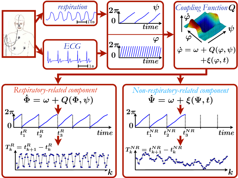
Figure 1: The approach at a glance. In the first step, instantaneous phases, $\varphi$ and $\psi$, are obtained from simultaneously measured ECG and respiratory signals. The cardiac phase $\varphi$ is defined in such a way that values $\varphi=2\pi k$ correspond to the R-peaks (wrapped definition of the phase is used here for better visibility). Next, the phase dynamics is reconstructed from data in the form of Eq. (6) with the coupling function $Q$ and the rest term $\xi$. This equation yields equations for instantaneous frequency of respiratory-related and non-respiratory-related components, i.e. for $\dot{\Phi}$ and $\dot{\Psi}$. Numerical integration of the latter equations provides phases of these components, while the conditions $\Phi(t_{k}^{R})=2\pi$ and $\Psi(t_{k}^{NR})=2\pi$ determine the newly generated series of R-peaks. As a final result we obtain tachograms for both components.

.

II.2 Reconstruction of the phase dynamics from data

We analyze below the set of 25 records of $420$ seconds long simultaneous measurements of respiratory flow and ECG, already explored for different purposes in the previous publication Kralemann_et_al-13 . The experiments were performed on healthy adults at rest, in a supine position. The details of the measurements, the preprocessing, and the subjects are described in the Supplementary Information to this paper and to Ref. Kralemann_et_al-13 .

Now we describe the particular steps behind the general disentanglement approach presented above. Since the representation of the cardiac dynamics via Eq. (6) has been derived in Kralemann_et_al-13 , here we only briefly outline the main steps.

1. Recorded cardiac ECG signals and respiratory signals have been embedded in a two-dimensional plane by virtue of the Hilbert transform. The protophase (phase-like variable) of the respiratory signal has been obtained as an angle in this plane. The protophase of the ECG signal required an extended processing, because this signal has a complex form with several loops over a basic cycle. In fact, in these approaches the details of parameterisation which may influence the definition of a protophase are not important, as is explained in the next lines.

2. A transformation from the protophases to the phases has been performed, according to the method suggested in Ref. Kralemann-08 . The main idea is that because the embedding and the parameterisation of the embedded trajectory by a $2\pi$-periodic phase-like variable are not unique, the obtained protophase is not unique too. The true phase is determined to have the property of growing linearly in time in absence of external forces (cf. Eq. (1) which is written for the true phase and thus the deterministic part of the r.h.s. does not depend on $\varphi$). We have performed an invertible deterministic transformation from the protophase to the phase (Eq. (4) in Ref. Kralemann_et_al-13 ), based on the property that the probability distribution density of the phase should be uniform.

3. Having now the time series of the true phases of the cardiac system, $\varphi(t)$, and of the respiratory one, $\psi(t)$, we have calculated the time derivative $\dot{\varphi}$ and have fitted it according to Eq. (6) with a function, which is $2\pi$-periodic in arguments $\varphi,\psi$. Practically, a kernel estimation (Eq. (7) in Ref. Kralemann_et_al-13 ) has been employed. As a result of this step, the basic Eq. (6) describing the cardiac phase dynamics is reconstructed.

II.3 Characterization of original and disentangled HRV data

In order to quantify the original RR-intervals and the results of the disentanglement procedure, we computed for all 25 data sets several physiologically relevant measures that are commonly used in HRV analysis.

The statistical measure in time-domain that directly characterizes the “evenness” of the sequence of RR intervals, is RMSSD: root mean square of successive differences Guidelines1996 , defined as

$$\text{RMSSD}=\sqrt{\langle|T_{k+1}-T_{k}|^{2}\rangle}\;.$$

Another measure, LogRSA Lehofer1997 , is defined as logarithm of the median of the distribution of the absolute values of successive differences, i.e.

$$\text{LogRSA}=\log\left[\text{median}|T_{k+1}-T_{k}|\right]$$

LogRSA takes care for a nearly log-normal statistical distribution of the medians, so that by taking logarithm a nearly normal distribution is achieved. Several studies Lehofer1999 ; Lehofer1997 ; Grote2007 ; Moser1998 have proven robustness of LogRSA and its ability to differentiate between vagal states. Another characteristics of “non-evenness” of RR interval series used especially in clinical settings is the relative (i.e. divided by the total number of the RR intervals in the time series) number of successive pairs of RR-intervals, that differ by more than 50 ms, denoted as pNN50 Guidelines1996 . Finally, we compute the standard deviation of RR intervals, SDNN.

In the frequency domain methods based on the power spectral density of the time series of RR intervals, one commonly computes the power in three frequency bands: VLF (very low frequency, from 0.0033 to 0.04 Hz), LF (low frequency, from 0.04 to 0.15 Hz), and HF (high frequency, from 0.15 to 0.4 Hz), e.g. by Fourier analysis.

Moreover, many nonlinear measures, mainly based on dynamical system approaches, have been applied to characterize HRV. Some of these measures require rather long time series and are therefore not applicable to our relatively short observations. As appropriate indices we have calculated the approximate entropy (ApEn) Pincus1991a ; Pincus1991b and the sample entropy (SampEn) Richman-Moorman-00 ; Chen_etal-09 of the HRV time series. (The tolerance value was taken as 15% of the standard deviation and the embedded dimension was fixed at 2.)

III Results

III.1 Time series and spectra

First, we illustrate the method, presenting the original HRV series $T_{k}$ along with the disentangled components $T_{k}^{R},T_{k}^{NR}$ in Fig. 2(a,c,e,g). In each panel these three series are shown by different colors and markers, and additionally shifted vertically for better visibility. We have chosen for presentation these four characteristic cases, while all studied cases are presented in the Supplementary Material. In all the cases, the original HRV time series show different extent of interval-to-interval variability. The R-HRV time series also show significant variability; these time series are however much more homogeneous just by their construction: the term $Q$ in Eq. (8) has a definite constant amplitude which is reflected in the magnitude of the variations of the R-HRV component. However, one can see clear differences in the NR-HRV series, obtained via Eq. (9). Now we go beyond visual inspection and quantify the components.

Basically, we can distinguish two types of the NR-HRV data: “smooth” and “rough”. In the former case, the differences between successive RR intervals are small, and the whole graph looks like a curve, possibly slightly perturbed. To this case belongs Fig. 2(e). In the “rough” case, the differences between the subsequent intervals are large, and one does not see a curve, but rather a dispersed set of points (panel (a)). There are also intermediate cases, like in panel (c). Finally, in panel (g) we show a remarkable NR-HRV pattern, consisting of “smooth” patches interrupted nearly periodically (approx. at every 30-th heart beat) by “rough” bursts.

A complementary information is contained in the power spectra of the HRV records, computed according to the procedure described in Clifford2005 and shown in the right column of Fig. 2. One can clearly recognize several characteristic features:

1. The respiratory-related R-HRV component has pronounced peaks. These peaks can be interpreted as the main frequency of respiration, its harmonics and the combinational harmonics, i.e. heartbeat frequency $\pm$ respiration frequency.

2. The NR-HRV part contains no pronounced peaks. This confirms that the main regular oscillatory contribution to the HRV is the respiration; all other perturbations are rather noisy and do not exhibit noticable spectral peaks (for the case depicted in panels (g,h), the low-frequency periodicity cannot be resolved in the power spectrum for such a short time series).

3. The R-HRV component has low values at frequencies smaller than that of respiration. In fact, at these frequencies, the spectra of the original HRV and of the NR-HRV practically coincide. This means that the slow irregular variability of the heart rhythm is mainly caused not by respiration, but by other physiological processes. Our disentanglement allows one to study these slow components in a reliable way, by cleansing the respiratory component that may hide the interesting slow processes.

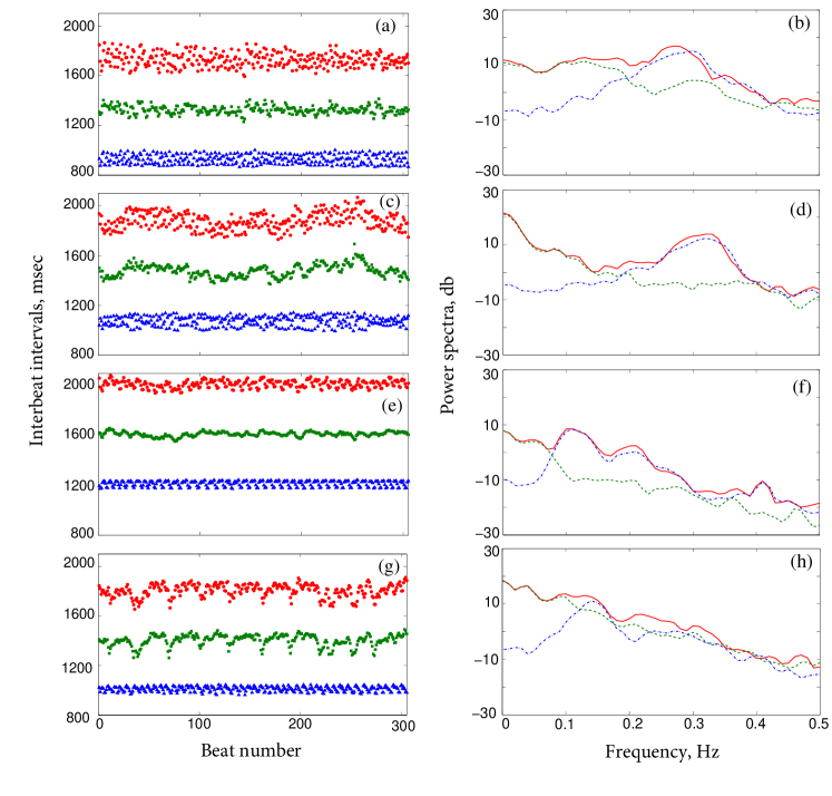
Figure 2: HRV plots (left column) and corresponding power spectral densities (right column). Original tachogram (red circles) is shown along with its R-HRV (blue triangles) and NR-HRV components (green squares). The corresponding spectra are given by red solid, blue dot-dashed, and green dashes lines, respectively. Left, for better visibility, RR intervals for NR-HRV component and for the original time series are shifted vertically by 400 ms and 800 ms, respectively. For the same reason only 300 beats are shown in tachograms; full records are shown in Supplementary Material. For discussion, see text.

For another illustration of the disentanglement we plot in Fig. 3 the original series and two constructed components components vs time, i.e. $T_{k}=t_{k+1}-t_{k}$ vs $t_{k+1}$, $T_{k}^{R}=t_{k+1}^{R}-t_{k}^{R}$ vs $t_{k+1}^{R}$, and $T_{k}^{NR}=t_{k+1}^{NR}-t_{k}$ vs $t_{k+1}^{NR}$, for one data set. Here we also show the time course of respiration, plotting $\cos\psi$ vs time. One can see that though the R-peaks in the HRV (filled circles) and in R-HRV (triangles) series occur at different instants of time, the overall pattern of the modulation by respiration, i.e. positions of peaks and troughs in the tachograms, is preserved.

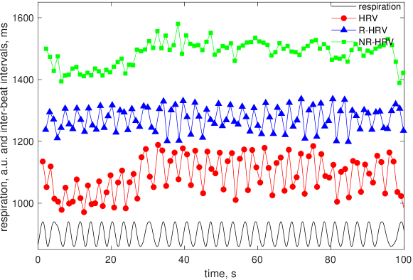
Figure 3: Example of the original HRV and its respiratory and non-respiratory related components. The latter two are shifted upwards for better visibility by 200 ms and 400 ms, respectively. Black curve shows respiratory signal with the amplitude normalized to one.

III.2 Time-domain characterizations of HRV

Figure 4(a) shows the RMSSD measure for both disentangled components of all data sets. We see that the RMSSD values for both the respiratory $\text{RMSSD}^{R}$ and non-respiratory $\text{RMSSD}^{NR}$ components are smaller than for the original one. We have found that in almost all cases, the reduction for the non-respiratory component is much stronger than for the respiratory one. One can see that the relative reduction of the RMSSD both for the R-HRV component (on average by factor 0.8) and NR-HRV component (on average by factor 0.5) does not depend on the RMSSD value for the original HRV series. Panel (b) of the same figure presents the pNN50 measure of “non-smoothness” of RR interval series. One can see that this quantity is significantly reduced for the NR-HRV component, while its value for the R-HRV component is nearly the same as for original data. (Exception are cases where pNN50 in the original time series is very small, here the successive pairs with RR intervals larger than 50 ms are nearly eliminated both in the R-HRV and NR-HRV components). Panel (c) if Fig. 4 shows the values of the measure logRSA. Reduction of this measure in the NR-HRV component is even more evident than in panels (a,b). Finally, panel (d) demonstrates that both components of the SDNN measure are reduced.

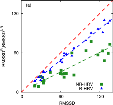
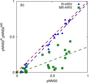
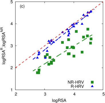
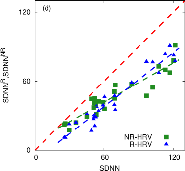
Figure 4: (a): The values $\text{RMSSD}^{R}$ and $\text{RMSSD}^{NR}$ versus RMSSD. (b): The values of $\text{pNN50}^{NR}$ and $\text{pNN50}^{R}$ vs pNN50. (c): The values of $\text{logRSA}^{NR}$ and $\text{logRSA}^{R}$ vs logRSA. (d): The values of $\text{SDNN}^{NR}$ and $\text{SDNN}^{R}$ vs SDNN. For clarity, the line of identity is shown by the red dashed line. Other dashed lines show linear fits (the slopes and corresponding correlation coefficients are given in square brackets): $\text{RMSSD}^{\text{NR-HRV}}$: $[0.50,0.90]$; $\text{RMSSD}^{\text{R-HRV}}$: $[0.90,0.99]$; $\text{pNN50}^{\text{NR-HRV}}$: $[0.38,0.72]$; $\text{pNN50}^{\text{R-HRV}}$: $[1.03,0.99]$; $\text{logRSA}^{\text{NR-HRV}}$: $[0.81,0.85]$; $\text{logRSA}^{\text{R-HRV}}$: $[1.09,0.97]$; $\text{SDNN}^{\text{NR-HRV}}$: $[0.57,0.93]$; $\text{SDNN}^{\text{R-HRV}}$: $[0.78,0.96]$.

III.3 Frequency-domain characterizations of HRV

The frequency-domain measures are plotted in Fig. 5. Here we show the power in three frequency bands for R-HRV and NR-HRV series versus the corresponding powers of the original HRV (cf. dashed line which is the diagonal in the log-log representation). The VLF component (panel (a)) is strongly reduced in the R-HRV, while it is nearly the same as the original one in the NR-HRV. This is a clear indication that the very low-frequency variability on time scales larger than 20 s is not due to the respiration, but is caused by other physiological and external influences. Noteworthy, the results for the VLF component are not very reliable due to a shortness of the time series in our measurements.

In the low-frequency range (roughly time scales from 25 to 6 s, panel (b)) the reduction in the R-HRV component is not so strong. In fact, for some subjects the R-HRV component is even higher than the NR-HRV component. It is known from literature that slow respiration largly enhances HRV at 6 breaths per minute where other LF rhythms are met Russo2017 . The high-frequency range (panel (c), time scales from 6 to 2 s) includes a typical period of breathing. Therefore, here the situation is the opposite to the cases of lower frequencies: the respiration component is only slightly less than the original one, while the NR-HRV component is stronger reduced.

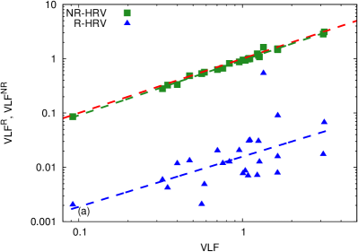
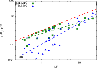
Figure 5: Spectral power in very-low-frequency (a), low-frequency (b), and high-frequency (b) spectral ranges. Here the R-HRV and NR-HRV components are shown vs the value of the corresponding power in the original time series. The red dashed line shows the diagonal, i.e. the values for the original time series). Other dashed lines show the power law fits (the correlation coefficients for the fits are given in square brackets): $\text{VLF}^{\text{NR-HRV}}\approx 0.93\cdot(\text{VLF})^{1.01}$ [0.97]; $\text{VLF}^{\text{R-HRV}}\approx 0.016\cdot(\text{VLF})^{0.92}$ [0.58]; $\text{LF}^{\text{NR-HRV}}\approx 0.6\cdot(\text{LF})^{0.77}$ [0.84]; $\text{LF}^{\text{R-HRV}}\approx 0.12\cdot(\text{LF})^{1.40}$ [0.79]; $\text{HF}^{\text{NR-HRV}}\approx 0.20\cdot(\text{HF})^{1.02}$ [0.91]; $\text{HF}^{\text{R-HRV}}\approx 0.70\cdot(\text{HF})^{0.98}$ [0.99].

III.4 Complexity measures

Finally, we present the results of computation of complexity measures ApEn and SampEn. Both entropies show similar behavior: their values for both R-HRV and NR-HRV are smaller then the entropy values of the original HRV signals, what means that the complexity of the total HRV is larger than that of its components. In almost all cases the NR-HRV signal shows larger regularity than the R-HRV component.

Figure 6: Values of the approximate entropy (a) and of the sampled entropy (b) for the R-HRV and NR-HRV components, vs the values of these quantities in the original time series (red dashed line is the diagonal). Other dashed lines show the power law fits (the correlation coefficients for the fits are given in square brackets): $\text{ApEn}^{R}\sim\left(\text{ApEn}\right)^{1.09}$ [0.98]; $\text{ApEn}^{NR}\sim\left(\text{ApEn}\right)^{0.9}$ [0.84]; $\text{SampEn}^{R}\sim\left(\text{SampEn}\right)^{1.15}$ [0.98]; $\text{SampEn}^{NR}\sim\left(\text{SampEn}\right)^{1.03}$ [0.82]. One can see that for originally more complex signals (large values of SampEn and ApEn), reduction of complexity in the R-HRV component is smaller (the corresponding powers are larger than 1), but reduction in complexity in the NR-HRV component is larger (the powers are closer to 1).

IV Conclusions and discussion

We have presented and illustrated a nonlinear technique which enables disentanglement of the RR-intervals series into the respiratory-related component, R-HRV, and the rest, NR-HRV. The procedure can be performed if simultaneous measurements of an ECG and of a respiratory signal are available. Our method is based on the coupled oscillators model, and thus is inherently nonlinear. In particular, this means that our procedure is not a simple decomposition (in the sense of signal decomposition techniques), i.e. $\text{R-HRV}+\text{NR-HRV}\neq\text{HRV}$. The spectral analysis confirms methodical validity of our approach, demonstrating that the R-HRV component correctly describes peaks in the power spectra at the respiratory-related frequencies. We suggest to use this approach as a universal preprocessing technique which allows a researcher to concentrate on particular properties of the HRV data. Moreover, the technique can be used for investigation of other physiological rhythms if bivariate or multivariate measurements are available.

The results presented in Figs. 4-6 show that some HRV measures appear to be dominated by one of the components. So, Figs. 4b,c show that the values of $\text{logRSA}^{\text{R}}$ and of $\text{pNN50}^{\text{R}}$ are very close to logRSA and pNN50, respectively. (Fig. 5)a. In particular, this indicates that logRSA and pNN50 may be more efficient for quantification of the respiratory-related component than other measures, if raw data are used. However, pNN50 suffers from a saturation effect in subjects where HRV is generally low. However, verification of this hypothesis requires further analysis with data from different groups of subjects. Moreover, Figs. 4-6 clearly demonstrate that generally computation of standard HRV measures from original data and its disentangled components yield different results, and this difference can be essential.

We notice that the technique requires rather high-quality ECG records and quite a demanding preprocessing, related to the phase estimation. Therefore we consider the current results as a “proof of principle”. A very useful practical improvement, now in progress, would be development of an approximate disentanglement algorithm that can be performed on the basis of RR-series only. Another essential potential development would be to incorporate into the model the amplitude variations of the respiratory signal, modifying Eq. (6) to

$$\dot{\varphi}=\omega+A(t)Q(\varphi,\psi)+\xi(\varphi,t)\;,$$ (10)

where $A(t)$ is the instantaneous amplitude that can be easily extracted by means of the Hilbert transform. However, for this purpose another type of measurements is required, where the amplitude of the measured respiratory signal can be attributed to true amplitude of the respiratory force affecting the cardio-vascular system.

The new method promises an improved determination of vagal tone for medicine and prevention, based on elaborated mathematical decomposition of available data. It also allows for a better understanding of the non-respiratory components of HRV in general. The parasympathetic nervous system is an important part of our control center for silent inflammation (also coined “secret killer” by Time magazine Gorman2004 ). Cellular receptors allowing communication of autonomic nervous system and immune cells have been found in the past decade and vagal activity has been proven to control immune activity. Therefore, a noninvasive quantification of vagal tone will become important in several fields of medicine in the near future for diagnostic as well as therapeutic purposes. The method described in this paper might be a valuable contribution for such a highly desired accurate measurement tool. The amount of vagal tone describes the ability of the organism to recover after inflammatory states, condition very important not only for our well-being and healthy aging, but for the prevention of serious chronic diseases like atherosclerosis, neurodegenerative diseases or cancer. Application of the method to medical diagnostics requires, however, future measurements from the corresponding groups of patients.

V Acknowledgments

ÇT was financially supported by the European Union’s Horizon 2020 research and innovation programme under the Marie Sklodowska-Curie Grant Agreement No. 642563 (COSMOS). Development of methods presented in Section 2 was supported by the Russian Science Foundation under Grant No. 17-12-01534. We acknowledge helpful discussion with Prof. J. Schaefer.

References

- (1) P.G. Katona and F. Jih. Respiratory sinus arrhythmia: noninvasive measure of parasympathetic cardiac control. J. Applied Physiology, 39:801–805, 1975.
- (2) J.A. Hirsch and B. Bishop. Respiratory sinus arrhythmia in humans: how breathing pattern modulates heart rate. Am J Physiol., 241:H620–629, 1981.
- (3) J. Hayano, F. Yasuma, A. Okada, S. Mukai, and T. Fujinami. Respiratory sinus arrhythmia. Circulation, 94(4):842–847, 1996.
- (4) G.E. Billman. Heart rate variability – a historical perspective. Front Physiol., 2:86, 2011.
- (5) M. Moser, M. Lehofer, A. Sedminek, M. Lux, H. G. Zapotoczky, T. Kenner, and A. Noordergraaf. Heart rate variability as a prognostic tool in cardiology. a contribution to the problem from a theoretical point of view. Circulation, 90(2):1078–1082, 1994.
- (6) P.D. Larsen, Y.C. Tzeng, P.Y.W. Sin, and D.C. Galletly. Respiratory sinus arrhythmia in conscious humans during spontaneous respiration. Respir Physiol Neurobiol, 174:111–118, 2010.
- (7) A. Ben-Tal, S. S. Shamailov, and J. F. R. Paton. Evaluating the physiological significance of respiratory sinus arrhythmia: looking beyond ventilation–perfusion efficiency. The Journal of Physiology, 590(8):1989–2008, 2012.
- (8) M. Elstad, L. Walløe, N. L. A. Holme, E. Maes, and M. Thoresen. Respiratory sinus arrhythmia stabilizes mean arterial blood pressure at high-frequency interval in healthy humans. European Journal of Applied Physiology, 115(3), 2014.
- (9) M. Moser, M. Frühwirth, D. Messerschmidt, N. Goswami, L. Dorfer, F. Bahr, and G. Opitz. Investigation of a micro-test for circulatory autonomic nervous system responses. Frontiers in Physiology, 8(JUL):1–11, 2017.
- (10) D. Baylis, D. B Bartlett, H. P. Patel, and H. C Roberts. Understanding how we age: insights into inflammaging. Longevity & Healthspan, 2(1):8, 2013.
- (11) M. Lehofer, M. Moser, R. Hoehn-Saric, D. McLeod, G. Hildebrandt, S. Egner, B. Steinbrenner, P. Liebmann, and H. G. Zapotoczky. Influence of age on the parasympatholytic property of tricyclic antidepressants. Psychiatry Research, 85(2):199–207, 1999.
- (12) M. Lehofer, M. Moser, R. Hoehn-Saric, D. McLeod, P. Liebmann, B. Drnovsek, S. Egner, G. Hildebrandt, and H. G. Zapotoczky. Major depression and cardiac autonomic control. Biological psychiatry, 42(10):914–9, 1997.
- (13) U. N. Das. Is obesity an inflammatory condition? Nutrition, 17(11-12):953–966, 2001.
- (14) K. J. Tracey. The inflammatory reflex. Nature, 420(6917):853–9, 2002.
- (15) C. Nathan. Points of control in inflammation. Nature, 420(6917):846–852, 2002.
- (16) S. Laborde, E. Mosley, and J. F. Thayer. Heart rate variability and cardiac vagal tone in psychophysiological research - Recommendations for experiment planning, data analysis, and data reporting. Frontiers in Psychology, 8(FEB):1–18, 2017.
- (17) G.F. Lewis, S.A. Furman, M.F. McCool, and S.W. Porges. Statistical strategies to quantify respiratory sinus arrhythmia: Are commonly used metrics equivalent? Biological Psychology, 89:349–364, 2012.
- (18) M.D. Wielgus, J.T. Aldrich, A.H.Mezulis, and S.E. Crowell. Respiratory sinus arrhythmia as a predictor of self-injurious thoughts and behaviors among adolescents. Int J Psychophysiol., 106:127–134, 2016.
- (19) C.J. Price and S.E. Crowell. Respiratory sinus arrhythmia as a potential measure in substance use treatment–outcome studies. Addiction, 111:615–625, 2016.
- (20) V. Panaite, A.C. Hindash, L.M. Bylsma, B.J. Small, K. Salomon, and J. Rottenberg. Respiratory sinus arrhythmia reactivity to a sad film predicts depression symptom improvement and symptomatic trajectory. Int J Psychophysiol, 99:108–113, 2016.
- (21) P. Grossman and E.W. Taylor. Toward understanding respiratory sinus arrhythmia: relations to cardiac vagal tone, evolution and biobehavioral functions. Biol Psychol, 74:263–285, 2007.
- (22) T. Ritz, M. Bosquet Enlow, S.M. Schulz, R. Kitts, J. Staudenmayer, and R.J. Wright. Respiratory sinus arrhythmia as an index of vagal activity during stress in infants: Respiratory influences and their control. PLoS ONE, 7:e52729, 2012.
- (23) M. Moser, M. Frühwirth, R. Penter, and R. Winker Why life oscillates - From a topographical towards a functional chronobiology. Cancer Causes and Control, 17(4):591–599, 2006.
- (24) P.Ch. Ivanov, L.A.N. Amaral, A. L. Goldberger, S. Havlin, M.G. Rosenblum, Z. Struzik, and H.E. Stanley. Multifractality in human heartbeat dynamics. Nature, 399(6735):461–465, 1999.
- (25) D.T. Schmitt and P.Ch. Ivanov. Fractal scale-invariant and nonlinear properties of cardiac dynamics remain stable with advanced age: a new mechanistic picture of cardiac control in healthy elderly. American Journal of Physiology-Regulatory, Integrative and Comparative Physiology, 293:R1923–R1937, 2007.
- (26) B. Kralemann, M. Frühwirth, A. Pikovsky, M. Rosenblum, T. Kenner, J. Schaefer, and M. Moser. In vivo cardiac phase response curve elucidates human respiratory heart rate variability. Nature Communications, 4:2418, 2013.
- (27) D. Widjaja, A. Caicedo, E. Vlemincx, I.Van Diest, and S. Van Huffel. Separation of respiratory influences from the tachogram: A methodological evaluation. PLOS ONE, 9(7):1–11, 07 2014.
- (28) J. Kuo and Ch.-D. Kuo. Decomposition of heart rate variability spectrum into a power-law function and a residual spectrum. Front. Cardiovasc. Med., 3:16, 2016.
- (29) A. T. Winfree. The Geometry of Biological Time. Springer, Berlin, 1980.
- (30) L. Glass. Synchronization and rhythmic processes in physiology. Nature, 410:277–284, 2001.
- (31) A. Pikovsky, M. Rosenblum, and J. Kurths. Synchronization. A Universal Concept in Nonlinear Sciences. Cambridge University Press, Cambridge, 2001.
- (32) S. H. Strogatz. Sync: The Emerging Science of Spontaneous Order. Hyperion, NY, 2003.
- (33) B. Kralemann, L. Cimponeriu, M. Rosenblum, A. Pikovsky, and R. Mrowka. Phase dynamics of coupled oscillators reconstructed from data. Phys. Rev. E, 77:066205, 2008.
- (34) Task Force of the European Society of Cardiology and the North American Society of Pacing and Electrophysiology. Heart rate variability. Standards of measurement, physiological interpretation, and clinical use. European Heart Journal, 17:354–381, 1996.
- (35) V. Grote, H. Lackner, C. Kelz, M. Trapp, F. Aichinger, H. Puff, and Max Moser. Short-term effects of pulsed electromagnetic fields after physical exercise are dependent on autonomic tone before exposure. European Journal of Applied Physiology, 101(4):495–502, 2007.
- (36) M. Moser, M. Lehofer, R. Hoehn-Saric, D. R. McLeod, G. Hildebrandt, B. Steinbrenner, M. Voica, P. Liebmann, and H. G. Zapotoczky. Increased heart rate in depressed subjects in spite of unchanged autonomic balance? Journal of Affective Disorders, 48(2-3):115–124, 1998.
- (37) S. M. Pincus, I. M. Gladstone, and R. A. Ehrenkranz. A regularity statistic for medical data analysis. Journal of Clinical Monitoring, 7(4):335–345, 1991.
- (38) S. M Pincus. Approximate entropy as a measure of system complexity. Mathematics, 88(March):2297–2301, 1991.
- (39) J. S. Richman and J. R. Moorman. Physiological time-series analysis using approximate entropy and sample entropy. Am. J. Physiol. Heart Circ. Physiol., 278:H2039–H2049, 2000.
- (40) W. Chen, J. Zhuang, W. Yu, and Z. Wang. Measuring complexity using FuzzyEn, ApEn, and SampEn. Med. Eng. Phys., 31:61–68, 2009.
- (41) G. D. Clifford and L. Tarassenko. Quantifying errors in spectral estimates of HRV due to beat replacement and resampling. IEEE Transactions on Biomedical Engineering, 52(4):630–638, 2005.
- (42) M. A. Russo, D. M. Santarelli, and D. O’Rourke. The physiological effects of slow breathing in the healthy human. Breathe (Sheff), 13(4):298-309, 2017.
- (43) C. Gorman, A. Park, and K. Dell. The silent killer. TIME, 2004.