Fast Influence Maximization in Dynamic Graphs:
A Local Updating Approach

Abstract.

We propose a generalized framework for influence maximization in large-scale, time evolving networks. Many real-life influence graphs such as social networks, telephone networks, and IP traffic data exhibit dynamic characteristics, e.g., the underlying structure and communication patterns evolve with time. Correspondingly, we develop a dynamic framework for the influence maximization problem, where we perform effective local updates to quickly adjust the top-$k$ influencers, as the structure and communication patterns in the network change. We design a novel N-Family method (N=1, 2, 3, $\ldots$) based on the maximum influence arborescence (MIA) propagation model with approximation guarantee of $(1-1/e)$. We then develop heuristic algorithms by extending the N-Family approach to other information propagation models (e.g., independent cascade, linear threshold) and influence maximization algorithms (e.g., CELF, reverse reachable sketch). Based on a detailed empirical analysis over several real-world, dynamic, and large-scale networks, we find that our proposed solution, N-Family improves the updating time of the top-$k$ influencers by $1\sim 2$ orders of magnitude, compared to state-of-the-art algorithms, while ensuring similar memory usage and influence spreads.

Abstract.

We propose a generalized framework for influence maximization in large-scale, time evolving networks. Many real-life influence graphs such as social networks, telephone networks, and IP traffic data exhibit dynamic characteristics, e.g., the underlying structure and communication patterns evolve with time. Correspondingly, we develop a dynamic framework for the influence maximization problem, where we perform effective local updates to quickly adjust the top-$k$ influencers, as the structure and communication patterns in the network change. We design a novel N-Family method (N=1, 2, 3, $\ldots$) based on the maximum influence arborescence (MIA) propagation model with approximation guarantee of $(1-1/e)$. We then develop heuristic algorithms by extending the N-Family approach to other information propagation models (e.g., independent cascade, linear threshold) and influence maximization algorithms (e.g., CELF, reverse reachable sketch). Based on a detailed empirical analysis over several real-world, dynamic, and large-scale networks, we find that our proposed solution, N-Family improves the updating time of the top-$k$ influencers by $1\sim 2$ orders of magnitude, compared to state-of-the-art algorithms, while ensuring similar memory usage and influence spreads.

1. Introduction

The problem of influence analysis (Kempe et al., 2003) has been widely studied in the context of social networks, because of the tremendous number of applications of this problem in viral marketing and recommendations. The assumption in bulk of the literature on this problem is that a static network has already been provided, and the objective is to identify the top-$k$ seed users in the network such that the expected number of influenced users, starting from those seed users and following an influence diffusion model, is maximized.

In recent years, however, people recognized the inherent usefulness in studying the dynamic network setting (Aggarwal and Subbian, 2014), and influence analysis is no exception to this general trend (Song et al., 2017; Ohsaka et al., 2016), because many real-world social networks evolve over time. In an evolving graph, new edges (interactions) and nodes (users) are continuously added, while old edges and nodes get dormant, or deleted. In addition, the communication pattern and frequency may also change.

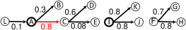
Figure 1. Running example: an influence graph

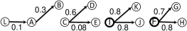
Figure 2. Influence graph after update operation: edge deletion $AC$

From an influence analysis perspective, even modest changes in the underlying network structure (e.g., addition/ deletion of nodes and edges) and communication patterns (e.g., update in influence probabilities over time) may lead to changes in the top-$k$ influential nodes. As an example, let us consider the influence graph in Figure 1 with 12 nodes, out of which the top-$2$ seed nodes are $A$ and $I$ (marked in bold), following the Maximum Influence Arborescence (MIA) model and $\theta=0.07$ (Chen et al., 2010) (we shall introduce the details of the MIA model later). The influence spread obtained from this seed set, according to the MIA model, is: $2.58+2.6=5.18$. Now, assume an update operation in the form of an edge removal $AC$ (marked in red). The new influence spread obtained from the old seed nodes would be: $1.3+2.6=3.9$, whereas if we recompute the top-$2$ seed nodes, they are $I$ and $F$, as shown in Figure 2. The influence spread from these new seed nodes is: $2.6+2.5=5.1$. It can be observed that there is a significant difference in the influence spread obtained with the old seed set vs. the new ones (even for such a small example graph), which motivates us to efficiently update the seed nodes when the influence graph evolves.

However, computing the seed set from ground, after every update, is prohibitively expensive (Song et al., 2017; Ohsaka et al., 2016) — this inspires us to develop dynamic influence maximization algorithms. By carefully observing, we realize that among the initial two seed nodes, only one seed node, namely $A$ is replaced by $F$, whereas $I$ still continues to be a seed node. It is because $A$ is in the affected region of the update operation, whereas $I$ is not affected by it. Therefore, if we can identify that $A$ can no longer continue as a seed node, then we can remove it from the seed set; and next, the aim would be to find one new seed node instead of two. Hence, we save almost $1/2$ of the computation in updating the seed set.

To this end, the two following questions are critical for identifying the top-$k$ seed nodes in a dynamic environment.

• What are the regions affected when the network evolves?

• How to efficiently update the seed nodes with respect to such affected regions?

Affected region. The foremost query that we address is identifying the affected region, i.e., the set of nodes potentially affected due to the update. They could be: (1) the nodes (including some old seed nodes) whose influence spreads are significantly changed due to the update operation, and also (2) those nodes whose marginal gains might change due to an affected seed node, discovered in the previous step(s). Given a seed set $S$, the marginal gain of a node $v\not\in S$ is computed as the additional influence that $v$ can introduce when it is added to the seed set.

Given the influence graph and dynamic updates, we design an iterative algorithm to quickly identify the nodes in the affected region. We call our method N-Family, $N=1,2,3,\ldots,$ (until a base condition is satisfied), which we shall discuss in Section 4.

Updating the seed nodes. Once the affected region is identified, updating the top-$k$ seed set with respect to that affected region is also a challenging problem. In this work, we develop an approximate algorithm under the MIA model of information diffusion, with theoretical performance guarantee of $1-1/e$.

Moreover, it should be understood that our primary aim is to maximize the influence spread as much as possible with the new seed nodes, instead of searching for the exact seed nodes (in fact, finding the exact seed nodes is $\mathbf{NP}$-hard (Kempe et al., 2003)). Therefore, we also show how to design more efficient heuristic algorithms, by carefully tuning the parameters (e.g., by limiting $N=2$) of our N-Family approach.

Our proposed framework to update the top-$k$ seed nodes is a generic one, and we develop heuristics by using it on top of other information propagation models (e.g., independent cascade, linear threshold (Kempe et al., 2003)) and several influence maximization (IM) algorithms (e.g., Greedy (Kempe et al., 2003), CELF (Leskovec et al., 2007), RR-sketch (Borgs et al., 2014; Tang et al., 2015)). In particular, we first find the affected region, and then update the seed nodes only by adding a few sub-routines to the existing static IM algorithms, so that they can easily adapt to dynamic changes.

Our contributions. The contributions of our work can be summarized as follows.

• We propose an iterative technique, N-Family that systematically identifies affected nodes (including old seed nodes) due to dynamic updates, and develop an incremental method that replaces the affected seed nodes with new ones, so to maximize the influence spread in the updated graph. We derive theoretical performance guarantees of our algorithm under the MIA model.

• We show how to develop efficient heuristics by extending proposed algorithm to other information propagation models and influence maximization algorithms for updating the seed nodes in an evolving network.

• We conduct a thorough experimental evaluation using several real-world, dynamic, and large graph datasets. The empirical results with our heuristics attest $1\sim 2$ orders of efficiency improvement, compared to state-of-the-art approaches (Song et al., 2017; Ohsaka et al., 2016). A snippet of our results is presented in Table 1.

Table 1. Average seed-set-updating time (sec) per node addition in the influence graph; the seed set consists of top-30 seed nodes; IC Model for influence cascade. For more details, we refer to Section 6.

Datasets	UBI+	Family-CELF	DIA	Family-RRS
(#nodes, #edges)	(Song et al., 2017)	[our method]	(Ohsaka et al., 2016)	[our method]
Digg (30K, 85K)	3.36 sec	0.008 sec	5.60 sec	0.20 sec
Slashdot (51K, 130K)	11.3 sec	0.05 sec	35.16 sec	2.96 sec
Epinions (0.1M, 0.8M)	1111.21 sec	24.58 sec	134.68 sec	5.31 sec
Flickr (2.3M, 33M)	45108.09 sec	1939.40 sec	770.41 sec	273.50 sec

2. Related Work

Kempe et al. (Kempe et al., 2003) addressed the problem of influence maximization in a social network as a discrete optimization problem, and proposed a hill climbing greedy algorithm, with an accuracy guarantee of $(1-1/e)$. They used the MC simulation to compute the expected influence spread of a seed set. Since the introduction of the influence maximization problem, many algorithms (see (Chen et al., 2013) for details) have been developed, both heuristic and approximated, to improve the efficiency of the original greedy method. Below, we survey some of these methods that are employed in our framework. Leskovec et al. (Leskovec et al., 2007) exploited the sub-modularity property of the greedy algorithm, and proposed more efficient CELF algorithm. Chen et al. (Chen et al., 2010) avoided MC simulations, and developed the MIA model using maximum probable paths for the influence spread computation. Addressing the inefficiency of MC simulations, Borgs et al. (Borgs et al., 2014) introduced a reverse reachable sketching technique (RRS) without sacrificing the accuracy guarantee.

In recent years, there has been interest in performing influence analysis in dynamic graphs (Aggarwal et al., 2012; Song et al., 2017; Liu et al., 2017; Zhuang et al., 2013; Ohsaka et al., 2016; Wang et al., 2017). The work in (Aggarwal et al., 2012) was the first to propose methods that maximize the influence over a specific interval in time; however, it was not designed for the online setting. The work in (Zhuang et al., 2013) probed a subset of the nodes for detecting the underlying changes. Liu et al. (Liu et al., 2017) considered an evolving network model (e.g., preferential attachment) for influence maximization. Subbian et al. (Subbian et al., 2016) discussed the problem of finding influencers in social streams, although they employed frequent pattern mining techniques over the underlying social stream of content. This is a different modeling assumption than the dynamic graph setting considered in this work. Recently, Wang et al. (Wang et al., 2017) considered a sliding window model to find influencers based on the most recent interactions. Once again, their framework is philosophically different from the classical influence maximization setting (Kempe et al., 2003), as they do not consider any edge probabilities; and hence, not directly comparable to ours.

In regards to problem formulation, recent works in (Song et al., 2017; Ohsaka et al., 2016; Yang et al., 2017) are closest to ours. UBI+ (Song et al., 2017) was designed for MC-simulation based algorithms and IC model. It performs greedy exchange for multiple times — every time an old seed node is replaced with the best possible non-seed node. If one continues such exchanges until there is no improvement, the method guarantees 0.5 approximation. DIA (Ohsaka et al., 2016) and (Yang et al., 2017) work on top of RR-Sketches. These methods generate all RR-sketches only once; and after every update, quickly modifies those existing sketches. After that, DIA (Ohsaka et al., 2016) identifies all seed nodes from ground using modified sketches. This is the key difference with our framework, since we generally need to identify only a limited number of new seed nodes, based on affected regions due to updates. On the contrary, (Yang et al., 2017) reports the top-$k$ nodes having maximum influence spreads individually with the modified sketches. Thus, the objective of (Yang et al., 2017) is different from that of classic influence maximization, which we study in this work.

Moreover, it is non-trivial to adapt both UBI+ and DIA for other influence models and IM algorithms, than their respective ones. A drawback of this is as follows. Sketch based methods (e.g., DIA) consume higher memory for storing multiple sketches. In contrast, MC-simulation based methods (e.g., UBI+) are slower over large graphs. On the other hand, our proposed N-Family approach can be employed over many IM models and algorithms, and due to the local updating principle, it significantly improves the efficiency under all scenarios. Therefore, one can select the underlying IM models and algorithms for the N-Family approach based on system specifications and application requirements. This demonstrates the generality of our solution.

3. Preliminaries

An influence network can be modeled as an uncertain graph $\mathcal{G}(V,E,$ $P)$, where $V$ and $E\subseteq V\times V$ denote the sets of nodes (users) and directed edges (links between users) in the network, respectively. $P$ is a function $P:E\rightarrow(0,1)$ that assigns a probability to every edge $uv\in E$, such that $P_{uv}$ is the strength at which an active user $u\in V$ influences her neighbor $v\in V$. The edge probabilities can be learnt (from past propagation traces), or inferred (following various models), as discussed in (Chen et al., 2013). In this work, we shall assume that $\mathcal{G}(V,E,P)$ is given as an input to our problem.

Algorithm 1 $Greedy(\mathcal{G},S,k)$: for IM in static networks

1:Graph $\mathcal{G}(V,E,P)$, seed set $S$ (initially empty), positive integer $k$

2:Seed set $S$ having the top-$k$ seed nodes

3:while $|S|<=k$ do

4:     $u^{*}=\operatorname*{arg\,max}_{u\in V\setminus S}\{\sigma(S\cup\{u\})-\sigma(S)\}$

5:     $S=S\cup u^{*}$

6:end while

7:Output $S$

3.1. Influence Maximization in Static Graphs

Whenever a social network user $u$ buys a product, or endorses an action (e.g., re-tweets a post), she is viewed as being influenced or activated. When $u$ is active, she automatically becomes eligible to influence her neighbors who are not active yet. While our designed framework can be applied on top of a varieties of influence diffusion models; due to brevity, we shall introduce maximum influence arborescence (MIA) (Chen et al., 2010) and independent cascade (IC) (Kempe et al., 2003) models. We develop an approximate algorithm with theoretical guarantee on top of MIA, and an efficient heuristic with IC.

MIA model. We start with an already active set of nodes $S$, called the seed set, and the influence from the seed nodes propagates only via the maximum influence paths. A path $Pt$ from a source $u$ to a destination node $v$ is called the maximum influence path $MIP(u,v)$ if this has the highest probability compared to all other paths between the same pair of nodes. Ties are broken in a predetermined and consistent way, such that the maximum influence path between a pair of nodes is always unique. Formally,

(1) $$MIP(u,v)=\operatorname*{arg\,max}_{Pt\in\mathcal{P}(u,v)}\{\prod_{e\in Pt}P_{e}\}\vspace{-2mm}$$

Here, $\mathcal{P}(u,v)$ denotes the set of all paths from $u$ to $v$. In addition, an influence threshold $\theta$ (which is an input parameter to trade off between efficiency and accuracy (Chen et al., 2010)) is used to eliminate maximum influence paths that have smaller propagation probabilities than $\theta$.

IC model. This model assumes that diffusion process from the seed nodes continue in discrete time steps. When some node $u$ first becomes active at step $t$, it gets a single chance to activate each of its currently inactive out-neighbors $v$; it succeeds with probability $P_{uv}$. If $u$ succeeds, then $v$ will become active at step $t+1$. Whether or not $u$ succeeds at step $t$, it cannot make any further attempts in the subsequent rounds. Each node can be activated only once and it stays active until the end. The campaigning process runs until no more activations are possible.

Influence estimation problem. All active nodes at the end, due to a diffusion process, are considered as the nodes influenced by $S$. In an uncertain graph $\mathcal{G}(V,E,P)$, influence estimation is the problem of identifying the expected influence spread $\sigma(S)$ of $S\subseteq V$.

It has been proved that the exact estimation of influence spread is a $\mathbf{\#P}$-hard problem, under the IC model (Chen et al., 2010). However, influence spread can be computed in polynomial time for the MIA model.

Marginal influence gain. Given a seed set $S$, the marginal gain $MG(S,u)$ of a node $u\not\in S$ is computed as the additional influence that $u$ can introduce when it is added to the seed set.

(2) $$MG(S,u)=\sigma(S\cup\{u\})-\sigma(S)$$

Influence maximization (IM) problem. Influence maximization is the problem of identifying the seed set $S^{*}$ of cardinality $k$ that has the maximum expected influence spread in the network.

Table 2. Notations used and their meanings

Symbol	Meaning
$\mathcal{G}(V,E,P)$	uncertain graph
$P_{e}$	probability of edge $e$
$Pt$	a path
$\mathcal{P}(u,v)$	set of all paths from $u$ to $v$
$MIP(u,v)$	the highest probability path from $u$ to $v$
$S$	seed set
$S^{i-1}$	seed set formed after $(i-1)$ iterations of Greedy algorithm
$s^{i}$	seed node added at the $i$-th iteration of Greedy algorithm
$\sigma(S)$	expected influence spread from $S$
$pp(S,u)$	probability that $u$ gets activated by $S$
$MG(S,u)$	marginal influence gain of $u$ w.r.t. seed set $S$
$Q$	priority queue that sorts non-seed nodes in descending order
	of marginal gains (w.r.t. seed set)

The influence maximization is an $\mathbf{NP}$-hard problem, under both MIA and IC models (Chen et al., 2010; Kempe et al., 2003).

In spite of the aforementioned computational challenges of influence estimation and maximization, the following properties of the influence function, $\sigma(S)$ assist us in developing a Greedy Algorithm (presented in Algorithm 1) with approximation guarantee of $(1-\frac{1}{e})$ (Kempe et al., 2003)

Lemma 1.

Influence function is sub-modular (Kempe et al., 2003; Chen et al., 2010). A function $f$ is sub-modular if $f(S\cup\{x\})-f(S)\geq f(T\cup\{x\})-f(T)$ for any $x$, when $S\subseteq T$.

Lemma 2.

Influence function is monotone (Kempe et al., 2003; Chen et al., 2010). A function $f$ is monotone if $f(S\cup\{x\})\geq f(S)$ for any x.

The Greedy algorithm repeatedly selects the node with the maximum marginal influence gain (line 2), and adds it to the current seed set (line 3) until $k$ nodes are identified.

As given in Table 2, we denote by $S^{i-1}$ the seed set formed at the end of the $(i-1)$-th iteration of Greedy, whereas $s_{i}\in S$ is the seed node added at the $i$-th iteration. Clearly, $1\leq i\leq k$. One can verify that the following inequality holds for all $i$, $1\leq i<k$.

(3) $$MG(S^{i-1},s^{i})\geq MG(S^{i},s^{i+1})\vspace{-1mm}$$

3.2. IM in Dynamic Graphs

Classical influence maximization techniques are developed for static graphs. The real-time influence graphs, however, are seldom static and evolves over time with various graph updates.

Graph update categories. We recognize six update operations among which four are edge operations and two are node operations in dynamic graphs: 1. increase in edge probability, 2. adding a new edge, 3. adding a new node, 4. decrease in edge probability, 5. deleting an existing edge, and 6. deleting an existing node. We refer to the first three update operations as additive updates, because the size of the graph and its parameters increase with these operations; and the remaining as reductive updates. Hereafter, we use a general term update for any of the above operations, until and unless specified, and we denote an update operation with $o$.

Dynamic influence maximization problem.

Problem 1.

Given an initial uncertain graph $\mathcal{G}(V,E,P)$, old set $S^{*}_{old}$ of top-$k$ seed nodes, and a series of consecutive graph updates $\{o_{1},o_{2},\ldots,o_{t}\}$, find the new set $S^{*}_{new}$ of top-$k$ seed nodes for this updated graph.

The baseline method to solve the dynamic influence maximization problem will be to find the updated graph at every time, and then execute an IM algorithm on the updated graph, which returns the new top-$k$ seed nodes. However, computing all seed nodes from ground at every snapshot is prohibitively expensive, even for moderate size graphs (Song et al., 2017; Ohsaka et al., 2016). Hence, our work aims at incrementally updating the seed set, without explicitly running the complete IM algorithm at every snapshot of the evolving graph.

4. Approximate Solution: MIA Model

We propose a novel N-Family framework for dynamic influence maximization, which can be adapted to many influence maximization algorithms and several influence diffusion models. We first introduce our framework under the MIA model that illustrates how an update affects the nodes in the graph (Section 4.1), and how to re-adjust the top-$k$ seed nodes with a theoretical performance guarantee (Section 4.2). Initially, we explain our technique for a single dynamic update, and later we show how it can be extended to batch updates (Section 4.3). In Section 5, we show how to extend our algorithm to IC and LT models, with efficient heuristics.

4.1. Finding Affected Regions

Given an update, the influence spread of several nodes in the graph could be affected. However, the nearby nodes would be impacted heavily, compared to a distant node. We, therefore, design a threshold ($\theta$)-based approach to find the affected regions, and our method is consistent with the notion of the MIA model. Recall that in MIA model, an influence threshold $\theta$ is used to eliminate maximum influence paths that have smaller propagation probabilities than $\theta$. Clearly, $\theta$ is an input parameter to trade off between efficiency and accuracy, and its optimal value is decided empirically.

Problem 2.

Given an update operation $o$ in an uncertain graph $\mathcal{G}(V,E,P)$, find all nodes $v\in V$ for which the expected influence spread $\sigma(\{v\})$ is changed by at least $\theta$.

In MIA model, the affected nodes could be computed exactly in polynomial time (e.g., by exactly finding the expected influence spread of each node before and after the update, with the MIA model). In this work, we, however, consider a more efficient upper bounding technique as discussed next.

4.1.1. Definitions

We start with a few definitions.

Definition 1 (Maximum Influence In-Arborescence).

Maximum Influence In-Arborescence (MIIA) (Chen et al., 2010) of a node $u\in V$ is the union of all the maximum influence paths to $u$ where every node in that path reaches $u$ with a minimum propagation probability of $\theta$, and it is denoted as $MIIA(u,\theta)$. Formally,

(4) $$MIIA(u,\theta)=\underset{v\in V}{\cup}\{MIP(v,u):\prod_{e\in MIP(v,u)}P_{e}\geq\theta\}$$

Definition 2 (Maximum Influence Out-Arborescence).

Maximum Influence Out-Arborescence (MIOA) (Chen et al., 2010) of a node $u\in V$ is the union of all the maximum influence paths from $u$ where $u$ can reach every node in that path with a minimum propagation probability of $\theta$, and it is denoted as $MIOA(u,\theta)$.

(5) $$MIOA(u,\theta)=\underset{w\in V}{\cup}\{MIP(u,w):\prod_{e\in MIP(u,w)}P_{e}\geq\theta\}$$

Definition 3 (1-Family).

For every node $u\in V$, 1-Family of $u$, denoted as $F_{1}(u)$, is the set of nodes that influence $u$, or get influenced by $u$ with minimum probability $\theta$ through the maximum influence paths, i.e.,

(6) $$F_{1}(u)=MIIA(u,\theta)\cup MIOA(u,\theta)$$

Definition 4 (2-Family).

For every node $u\in V$, 2-Family of $u$, denoted as $F_{2}(u)$, is the union of the set of nodes present in 1-Family of every node in $F_{1}(u)$, i.e.,

(7) $$F_{2}(u)=\underset{w\in F_{1}(u)}{\cup}{F_{1}(w)}$$

Note that 2-Family is always a superset of 1-Family of a node.

Example 1.

In Figure 1, let us consider $\theta=0.07$. Then, $pp(\{C\},$ $C)=1,pp(\{A\},C)=0.8$, and $pp(\{L\},C)=0.8\times 0.1=0.08$. For any other node in the graph, its influence on $C$ is 0. Hence, $MIIA(C,0.07)=\{C,A,L\}$. Similarly, $MIOA(C,0.07)=\{C,D,E\}$. $F_{1}(C)$ will contain $\{C,A,L,D,E\}$. Analogously $F_{2}(C)$ will contain $\{C,A,L,D,E,B\}$. Since the context is clear, for brevity we omit $\theta$ from the notation of family.

We note that Dijkstra’s shortest path algorithm, with time complexity $\mathcal{O}(|E|+|V|\log|V|)$ (Chen et al., 2010), can be used to identify the $MIIA$, $MIOA$, and 1-Family of a node. The time complexity for computing 2-Family is $\mathcal{O}(|E|+|V|\log|V|)^{2}$. For simplicity, we refer to 1-Family of a node as its family.

The 2-Family of a seed node satisfies an interesting property (given in Lemma 3) in terms of marginal gains.

Lemma 3.

Consider $s\in S$, then removing $s$ from the seed set $S$ does not change the marginal gain of any node that is not in $F_{2}(s)$. Formally, $MG(S,u)=MG(S\setminus\{s\},u)$, for all $u\in V\setminus F_{2}(s)$, according to the MIA model.

Formal proofs of all our lemma and theorems are given in the Appendix. Intuitively, Lemma 3 holds because the marginal gain of a node $u$ depends on the influence of seed nodes over those nodes that $u$ influences. For a node $u$ that is outside $F_{2}(s)$, there is no node that can be influenced by both $s$ and $u$. It follows from the fact that a node influences, or gets influenced by the nodes that are present only in its family, based on the MIA model.

Change in family after an update. During the additive update, e.g., an edge addition, the size of the family of a node nearby the update may increase. A new edge would help in more influence spread, as demonstrated below.

Example 2.

Consider Figure 2 as the initial graph. When $\theta=0.07$, $F_{1}(A)=\{A,L,B\}$. Let us assume that a new edge $AC$ with probability $0.8$ is added, that is, the updated graph is now Figure 1. If we recompute $F_{1}(A)$ in Figure 1, then we get $F_{1}(A)=\{A,B,C,D,L\}$.

Analogously, during the reductive update, e.g., an edge deletion, the size of family of a node surrounding the update may decrease. Deleting the edge eliminates paths for influence spread, as follows.

Example 3.

Consider Figure 1 as the initial graph. $F_{1}(A)=\{A,B,C,$ $D,L\}$. Now, the edge $AC$ with probability $0.8$ is deleted. If we recompute $F_{1}(A)$ after modifying the graph (i.e., Figure 2), we get $F_{1}(A)=\{A,B,L\}$.

Thus, for soundness, in case of an additive update, we compute $MIIA$, $MIOA$, and family on the updated graph. On the contrary, for a reductive update, we compute them on the old graph, i.e., before the update. Next, we show in Lemma 4 that $MIIA(u,\theta)$ provides a safe bound on affected region for any update originating at node $u$, according to the MIA model.

Lemma 4.

In an influence graph $\mathcal{G}(V,E,P)$, adding a new edge $uv$ does not change the influence spread of any node outside $MIIA(u,$ $\theta)$ by more than $\theta$, according to the MIA model.

Lemma 4 holds because a node $u$ cannot be influenced by any node that is not in $MIIA(u,\theta)$, according to the MIA model. Hence, adding an edge $uv$ does not change the influence spread (at all) of any node outside $MIIA(u,\theta)$. This phenomenon can be extended to edge deletion, edge probability increase, and for edge probability decrease. Moreover, for a node update (both addition and deletion) $u$, $MIIA(u,\theta)$ gives a safe upper bound of the affected region. We omit the proof due to brevity. Therefore, $MIIA(u,\theta)$ is an efficient (computing time $\mathcal{O}(|E|+|V|\log|V|)$) and a safe upper bound for the affected region.

4.1.2. Infected Regions

Due to an update in the graph, we find that a node may get affected in two ways: (1) the nodes (including a few old seed nodes) whose influence spreads are significantly affected due to the update operation, and also (2) those nodes whose marginal gains might change due to an affected seed node, discovered in the previous step(s). This gives rise to a recursive definition, and multiple levels of infected regions, as introduced next.

First infected region (1-IR). Whenever an update operation $o$ takes place, the influence spread of the nodes surrounding it, will change. Hence, we consider the first infected region as the set of nodes, whose influence spreads change at least by $\theta$.

Definition 5 (First infected region (1-IR)).

In an influence graph $\mathcal{G}(V,E,P)$ and given a probability threshold $\theta$, for an update operation $o$, 1-IR$(o)$ is the set of nodes whose influence spread changes greater than or equal to $\theta$. Formally,

(8) $$\text{\sf 1-IR}(o)=\{v\in V:|\sigma_{\mathcal{G}}(v)-\sigma_{\mathcal{G},o}(v)|\geq\theta\}$$

In the above equation, $\sigma_{\mathcal{G}}(v)$ denotes the expected influence spread of $v$ in $\mathcal{G}$, whereas $\sigma_{\mathcal{G},o}(v)$ is the expected influence spread of $v$ in the updated graph. Following our earlier discussion, we consider $MIIA(u,\theta)$ as a proxy for 1-IR$(o)$, where $u$ is the starting node for the update operation $o$.

Example 4.

In Figure 1, consider the removal of edge $AC$. Assuming $\theta=0.07$, 1-IR$(o)$=$MIIA(A,0.07)=\{A,L\}$.

Second infected region (2-IR). We next demonstrate how infection propagates from the first infected region to other parts of the graph through the family of affected seed nodes.

First, consider a seed node $s\in S$, a non-seed node $u\not\in S$, and $s\in F_{2}(u)$. If the influence spread of $u$ has increased due to an update, then to ensure that $s$ continues as a seed node, we have to remove $s$ from the seed set, and recompute the marginal gain of every node in $F_{2}(s)$. The node, which has the maximum gain, will be the new seed node. Second, if a seed node $s$ gets removed from the seed set in this process, the marginal gains of all nodes present in $F_{2}(s)$ will change. We are now ready to define the second infected region.

Definition 6 (Second infected region (2-IR)).

For an additive update $(o_{a})$, the influence spread of every node present in 1-IR$(o_{a})$ increases which gives the possibility for any node in 1-IR to become a seed node. Hence, the union of 2-Family of all the nodes present in 1-IR$(o_{a})$ is called the second infected region 2-IR$(o_{a})$. On the contrary, in a reductive update operation $o_{r}$, there is no increase in influence spread of any node in 1-IR$(o_{r})$. Hence, the union of 2-Family of old seed nodes present in 1-IR$(o_{r})$ is considered as the second infected region 2-IR$(o_{r})$.

(9) $$\text{\sf 2-IR}(o_{r})=\{F_{2}(s):s\in\text{\sf 1-IR}(o_{r})\cap S\}$$

(10) $$\text{\sf 2-IR}(o_{a})=\{F_{2}(u):u\in\text{ \sf 1-IR}(o_{a})\}$$

The time complexity to identify 2-IR is $\mathcal{O}(m(|E|+|V|\log|V|)^{2})$, where $m$ is the number of nodes in 1-IR.

Example 5.

In Figure 1, consider the removal of edge $AC$. Assuming $\theta=0.07$, 2-IR$(o)$=$F_{2}(A)$. This is because $A$ is an old seed node present in 1-IR$(o)$ for this reductive update. Furthermore, because this is a reductive update, the family of $A$ needs to be computed before the update. Therefore, 2-IR$(o)$=$F_{2}(A)=\{A,B,C,D,L,E\}$.

Iterative infection propagation. Whenever there is an update, the infection propagates through the 2-Family of the nodes whose marginal gain changes as discussed above. For $N\geq 3$, the infection propagates from the $(N-1)^{th}$ infected region to the $N^{th}$ infected region through old seed nodes that are present in the 2-Family of nodes in (N-1)-IR.

Definition 7 ($N(\geq 3)$ infected region (N-IR)).

The 2-Family of seed nodes, that are in the 2-Family of infected nodes in (N-1)-IR, constitute the $N^{th}$ infected region.

(11) $$\text{\sf N-IR}=\{F_{2}(s):s\in F_{2}(u)\cap S,u\in{\text{\sf(N-1)-IR}}\}$$

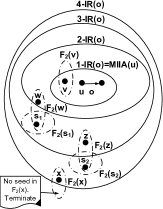
Figure 3. Iterative infection propagation: $o$ is an additive update operation originating at node $u$. $s_{1}$ and $s_{2}$ are two old seed nodes. $v$, $w$, $z$, $x$ are nodes, not necessarily old seed nodes.

We demonstrate the iterative computation of infected regions, up to 4-IR for an additive update, in Figure 3. We begin with node $u$ which is the starting node of the update, and $MIIA(u,\theta)$ is the 1-IR. The update being an additive one, union of 2-Family of all the nodes $v\in\text{\sf 1-IR}$ is considered as the 2-IR. For all nodes $w\in\text{\sf 2-IR}$, we compute $F_{2}(w)$. Now, union of 2-Family of all seed nodes $s_{1}\in F_{2}(w)$ is considered as 3-IR. Similarly, 4-IR can be deduced, and as there is no seed node present in the 2-Family of all nodes $x\in\text{\sf 4-IR}$, we terminate the infection propagation.

Termination of infection propagation. The infection propagation stops when no further old seed node is identified in the 2-Family of any node in the $N^{th}$ infected region. Due to this, there shall be no infected node present in 2-Family of any uninfected seed node. For a seed set of cardinality $k$, it can be verified that the maximum value of $N$ can be between $1$ and $(k+1)$ for reductive update and between $2$ and $(k+2)$ for additive update.

Total infected region (TIR). The union of all infected regions is referred to as the total infected region (TIR).

(12) $${\sf TIR}={\text{\sf 1-IR}}\cup{\text{\sf 2-IR}}\cup{\text{\sf 3-IR}}\cup\ldots\text{until termination}$$

Our recursive definition of TIR ensures the following properties.

Lemma 5.

The marginal gain of every node outside TIR does not change, according to the MIA model. Formally, let $S$ be the old seed set, and we denote by $S_{rem}$ the remaining old seed nodes outside TIR, i.e., $S_{rem}=S\setminus{\text{\sf TIR}}$. Then, the following holds: $MG(S,v)=MG(S_{rem},v)$, for all nodes $v\in V\setminus{\text{\sf TIR}}$.

Lemma 5 holds because any node outside TIR does not belong to 2-Family of any seed node present in TIR. Hence, by Lemma 3, its marginal gain does not change.

Lemma 6.

Any old seed node outside TIR has no influence on the nodes inside TIR, following the MIA model. Formally, $pp(S_{rem},u)=0$, for all nodes $u\in{\text{\sf TIR}}$.

Lemma 6 holds because any uninfected seed node is more than 2-Family away from any node present in TIR (This is how we terminate infection propagation). Hence, there is no node present in TIR that belongs to the family of any seed node outside TIR.

Algorithm 2    N-Family seeds updating method on top of Greedy

1:Graph $\mathcal{G}(V,E,P)$, total infected region TIR, old seed set $S$, $|S|=k$, old priority queue $Q$

2:Compute the new seed set $S_{new}$ of size $k$

3:$S_{rem}\leftarrow S\setminus{\sf TIR}$

4:for all $u\in{\sf TIR}$ do

5:     $Q(u)\leftarrow\sigma(u)$

6:end for

7:while TRUE do

8:     $S_{new}=$ Greedy$(\mathcal{G},S_{rem},k)$

9:/* Starting w/ seed set $S_{rem}$, add $k-|S_{rem}|$ seeds by Greedy */ 

10:     $S_{order}\leftarrow$ Sort nodes in $S_{new}$ in Greedy inclusion order

11:     $w\leftarrow Q$[top]

12:     if $(S^{k-1}_{order},s^{k}_{o})<MG(S_{order},w)$ then

13:         for all $u\in F_{2}(s^{k}_{o})\setminus S^{k-1}_{order}$ do

14:              $Q(u)\leftarrow MG(S^{k-1}_{order},u)$

15:              $S_{rem}\leftarrow S^{k-1}_{order}$

16:         end for

17:     else

18:         Output $S_{order}$

19:     end if

20:end while

The old seed nodes inside TIR may no longer continue as seeds, therefore we need to discard them from the seed set, and the same number of new seed nodes have to be identified. We discuss the updating procedure of seed nodes in the following section.

4.2. Updating the Seed Nodes

We now describe our seed updating method over the Greedy IM algorithm, under the MIA model of influence cascade. Later we prove that the new seed nodes reported by our technique (Algorithm 2) will be the same as the top-$k$ seed nodes found by Greedy on the updated graph and with the MIA model, thereby maintaining $(1-\frac{1}{e})$ approximation guarantee to the optimal solution (Chen et al., 2010).

4.2.1. Approximation Algorithm

We present our proposed algorithm for updating the seed set in Algorithm 2. Consider Greedy (Algorithm 1) over the MIA model on the initial graph, and assume that we obtained the seed set $S$, having cardinality $k$. Since Greedy works in an iterative manner, let us denote by $S^{i-1}$ the seed set formed at the end of the $(i-1)$-th iteration, whereas $s_{i}\in S$ is the seed node added at the $i$-th iteration. Clearly, $1\leq i\leq k$, $|S^{i-1}|=i-1$, and $S=S^{k}=\cup_{i=1}^{k}s_{i}$. Additionally, we use a priority queue $Q$, where its top node $w$ has the maximum marginal gain $MG(S,w)$ among all the non-seed nodes.

After the update $o$, we first compute the total infected region, TIR using Equation 12. Consider $S_{rem}$, of size $|S_{rem}|=k^{\prime}$, as the set of old seed nodes outside TIR, i.e., $S_{rem}=S\setminus{\text{\sf TIR}}$. Then, we remove $(k-k^{\prime})$ old seed nodes inside TIR, and our next objective is to identify $(k-k^{\prime})$ new seed nodes from the updated graph.

Note that inside $S_{rem}$, the seed nodes are still sorted in descending order of their marginal gains, computed at the time of insertion in the old seed set $S$ following the Greedy algorithm. In particular, we denote by $s_{r}^{j}$ the $j$-th seed node in descending order inside $S_{rem}$, where $1\leq j\leq k^{\prime}$. Due to Lemma 5, $MG(S,v)=MG(S_{rem},v)$, for all nodes $v\in V\setminus{\text{\sf TIR}}$. Thus, for all $j$, $1\leq j<k^{\prime}$ the following inequalities hold.

(13) $$MG(S_{rem}^{j-1},s_{r}^{j})\geq MG(S_{rem}^{j},s_{r}^{j+1})$$

(14) $$MG(S_{rem}^{k^{\prime}-1},s_{r}^{k^{\prime}})\geq MG(S_{rem}^{k^{\prime}-1},v)$$

Now, after removing the old seed nodes present in TIR from the seed set, we compute the influence spread $\sigma(u)$ of every node $u\in{\text{\sf TIR}}$ and, we update these nodes $u$ in the priority queue $Q$, based on their new marginal gains $\sigma(u)$ (lines 1-4). It can be verified that $MG(S_{rem},u)=\sigma(u)$, for all $u\in{\text{\sf TIR}}$, due to Lemma 6.

Now, we proceed with greedy algorithm and find the new $(k-k^{\prime})$ seed nodes. Let us denote by $S_{new}$ the new seed set (of size $k$) found in this manner (line 6). Next, we sort the seed nodes in $S_{new}$ in their appropriate inclusion order according to the Greedy algorithm over the updated graph (line 7). This can be efficiently achieved by running Greedy only over the seed nodes in $S_{new}$, while computing their influence spreads and marginal gains in the updated graph. The sorted seed set is denoted by $S_{order}$. Let us denote by $s_{o}^{k}$ the last (i.e., $k$-th) seed node in $S_{order}$, whereas $S_{order}^{k-1}$ represents the set of top-$(k-1)$ seed nodes in $S_{order}$. We denote by $w$ the top-most seed node in the priority queue $Q$. If $MG(S_{order}^{k-1},s_{o}^{k})\geq MG(S_{order},w)$, we terminate our updating algorithm (line 15).

Iterative seed replacement. On the other hand, if $MG(S_{order}^{k-1},s_{o}^{k})<MG(S_{order},w)$, we remove the last seed node $s_{o}^{k}$ from $S_{order}$. For every node $u$ in the $F_{2}(s_{o}^{k})\setminus S_{order}^{k-1}$, we compute marginal gain $MG(S_{order}^{k-1},u)$ and update the priority queue $Q$ (lines 10-11). Next, we compute a new seed node using Greedy and add it to $S_{order}^{k-1}$, thereby updating the seed set $S_{order}$. We also keep the nodes in $S_{order}$ sorted after every update in it. Now, we again verify the condition: if $MG(S_{order}^{k-1},s_{o}^{k})<MG(S_{order},w)$, where $w$ being the new top-most node in the priority queue $Q$, then we repeat the above steps, each time replacing the last seed node $s_{o}^{k}$ from $S_{order}$, with the top-most node from the updated priority queue $Q$. This iterative seed replacement phase terminates when $MG(S_{order}^{k-1},s_{o}^{k})\geq MG(S_{order},w)$. Clearly, this seed replacement can run for at most $|S_{rem}|=k^{\prime}$ rounds; because in the worst scenario, all old seed nodes in $S_{rem}$ could get replaced by new seed nodes from TIR. Finally, we report $S_{order}$ as the new seed set.

4.2.2. Theoretical Performance Guarantee

We show in the Appendix that the top-$k$ seed nodes reported by our N-Family method are the same as the top-$k$ seed nodes obtained by running the Greedy on the updated graph under the MIA model. Since, the Greedy algorithm provides the approximation guarantee of $1-\frac{1}{e}$ under the MIA model (Chen et al., 2010), our N-Family also provides the same approximation guarantee.

4.3. Extending to Batch Updates

We consider the difference of nodes and edges present in two snapshots at different time intervals of the evolving network as a set of batch updates. Clearly, we consider only the final updates present in the second snapshot, avoiding the intermediate ones. For example, in between two snapshot graphs, if an edge $uv$ is added and then gets deleted, we will not consider it as an update because there is no change in the graph with respect to $uv$ after the final update.

One straightforward approach would be to apply our algorithm for every update sequentially. However, we develop a more efficient technique as follows. For a batch update consisting of $m$ individual updates, every update $o_{i}$ has its own TIR$(o_{i}),i=1,2,3,\ldots,m$. The TIR of the batch update is the union of TIR$(o_{i})$, for all $i\in(1,m)$.

(15) $$\displaystyle\text{\sf TIR}=\cup_{i=1}^{m}\text{\sf TIR}(o_{i})$$

Once the TIR is computed corresponding to a batch update, we update the seed set using Algorithm 2. Processing all the updates in one batch is more efficient than the sequential updates. For example, if a seed node is affected multiple times during sequential updates, we have to check if it remains the seed node every time. Whereas in batch update, we need to verify it only once.

5. Heuristic Solution: IC and LT models

Here, we will show how one can develop efficient heuristics by extending the proposed N-Family approach to IC and LT models (Kempe et al., 2003). We start with IC model.

Computing TIR. For IC model, one generally does not use any probability threshold $\theta$ to discard smaller influences; and perhaps more importantly, finding the nodes whose influence spread changes by at least $\theta$ (due to an update operation) is a $\mathbf{\#P}$-hard problem. Hence, computing TIR under IC model is hard as well, and one can no longer ensure a theoretical performance guarantee of $(1-\frac{1}{e})$ as earlier. Instead, we estimate TIR analogous to MIA model (discussed in Section 4.1.2), which generates high-quality results as verified in our detailed empirical evaluation. This is because the maximum influence paths considered by MIA model play a crucial role in influence cascade over real-world networks (Chen et al., 2010).

Updating Seed set. Our method for updating the seed set in IC model follows the same outline as given in Algorithm 2 with two major differences. In lines 3 and 11 of Algorithm 2, we compute the marginal gains and update the priority queue, but now we employ more efficient techniques based on the IM algorithm used for the purpose. In particular, as discussed next, we derive two efficient heuristics, namely, Family-CELF (or, F-CELF) and Family-RRS (or F-RRS) by employing our N-Family approach on top of two efficient IM algorithms CELF (Leskovec et al., 2007) and RR sketch (Borgs et al., 2014), respectively.

5.1. N-Family for IM Algorithms in IC model

First, we explain static IM algorithms briefly, and then we introduce the methods to adapt them to a dynamic setting.

5.1.1. CELF

In the Greedy algorithm discussed in Section 3, marginal influence gains of all remaining nodes need to be repeatedly calculated at every round, which makes it inefficient (see Line 3, Algorithm 1). However, due to the sub-modularity property of the influence function, the marginal gain of a node in the present iteration cannot be more than that of the previous iteration. Therefore, the CELF algorithm (Leskovec et al., 2007) maintains a priority queue containing the nodes and their marginal gains in descending order. It associates a flag variable with every node, which stores the iteration number in which the marginal gain for that node was last computed. In the beginning, (individual) influence spreads of all nodes are calculated and added to the priority queue, and flag values of all nodes are initiated to zero. In the first iteration, the top node in the priority queue is removed, since it has the maximum influence spread, and is added to the seed set. In each subsequent iteration, the algorithm takes the first element from the priority queue, and verifies the status of its flag. If the marginal gain of the node was calculated in the current iteration, then it is considered as the next seed node; else, it computes the marginal gain of the node, updates its flag, and re-inserts the node in the priority queue. This process repeats until $k$ seed nodes are identified.

FAMILY-CELF We refer to the N-Family algorithm over CELF as FAMILY-CELF (or, F-CELF). In particular, we employ MC-sampling to compute marginal gains in lines 3 and 11 of Algorithm 2, and then update the priority queue. Given a node $u$ and the current seed set $S$, the corresponding marginal gain can be derived with two influence spread computations, i.e., $\sigma(S\cup\{u\})-\sigma(S)$. However, thanks to the lazy forward optimization technique in CELF, one may insert any upper bound of the marginal gain in the priority queue. The actual marginal gain needs to be computed only when that node is in the top of the priority queue at a later time. Therefore, we only compute the influence spread of $u$, i.e., $\sigma(\{u\})$, which is an upper bound to its marginal gain, and insert this upper bound in the priority queue.

5.1.2. Reverse Reachable (RR) Sketch

In this method, first proposed by Borgs et al. (Borgs et al., 2014) and later improved by Tang et al. (Tang et al., 2015, 2014), subgraphs are repeatedly constructed and stored as sketches in index $\mathbb{I}$. For each subgraph $H_{i}$, an arbitrary node $z_{i}\in V$, selected uniformly at random, is considered as the target node. Using a reverse Breadth First Search (BFS) traversal, it finds all nodes that influence $z_{i}$ through active edges. An activation function $x_{i}:E\rightarrow(0,1)$ is selected uniformly at random, and for each edge $uv\in E$, if $x_{i}(uv)\leq P_{uv}$, then it is considered active. The subgraph $H_{i}$ consists of all nodes that can influence $z_{i}$ via these active edges. Each sketch is a tuple containing $(z_{i},x_{i},H_{i})$. This process halts when the total number of edges examined exceeds a pre-defined threshold $\tau=\Theta(\frac{1}{\epsilon^{2}}k(|V|+|E|)\log{|V|})$, where $\epsilon$ is an error function associated with the desired quality guarantee $(1-\frac{1}{e}-\epsilon)$. The intuition is that if a node appears in a large number of subgraphs, then it should have a high probability to activate many nodes, and therefore, it would be a good candidate for a seed node. Once the sufficient number of sketches are created as above, a greedy algorithm repeatedly identifies the node present in the majority of sketches, adds it to the seed set, and the sketches containing it are removed. This process continues until $k$ seed nodes are found.

FAMILY-RRS We denote the N-FAMILY algorithm over RR-Sketch as FAMILY-RRS (or, F-RRS). RRS technique greedily identifies the node present in the majority of sketches, adds it to the seed set, and the sketches containing it are deleted. This process continues until $k$ seed nodes are identified. In our F-RRS algorithm, instead of deleting sketches as above, we remove them from $\mathbb{I}$, and store them in another index $\mathbb{R}$, since these removed sketches could be used later in our seeds updating procedure.

Let $\mathbb{I}_{v}\subseteq\mathbb{I}$ be the set of sketches $(z,x,H)\in\mathbb{I}$ with $v\in H$. Similarly, $\mathbb{R}_{u}\subseteq\mathbb{R}$ represents the set of all sketches $(z,x,H)\in\mathbb{R}$ with $u\in H$. Furthermore, $\mathbb{I}^{S}$ (similarly $\mathbb{R}^{S}$) denotes $\mathbb{I}$ (similarly $\mathbb{R}$) after the seed set $S$ is identified. Clearly, the sketches in $\mathbb{I}^{S}$ will not have any seed node in their subgraphs. Also note that $MG(S,v)$ is proportional to $|\mathbb{I}^{S}_{v}|$, by following the RRS technique.

After an update operation, we need to modify the sketches (both in $\mathbb{I}$ and $\mathbb{R}$), and also to possibly swap some sketches between these two indexes, as discussed next.

Modifying sketches after dynamic updates. In the following, we only discuss sketch updating techniques corresponding to an edge addition. Sketch updating methods due other updates (e.g., node addition, edge deletion, etc.) are similar (Ohsaka et al., 2016), and we omit them due to brevity. To this end, we present three operations:

Expanding sketches: Assume that we added a new edge $uv$. We examine every sketch $(z,x,H)$ both in $\mathbb{I}^{S}_{v}$ and $\mathbb{R}^{S}_{v}$, and add every new node $w$ that can reach $v$ through active edges in $H$. We compute these new nodes using a reverse breadth first search from $v$. In this process, the initial subgraph $H$ is extended to $H^{e}$.

Next, we need to update $\mathbb{I}^{S}$ and $\mathbb{R}^{S}$ in such a way that sketches in $\mathbb{I}^{S}$ do not have a seed node in their (extended) subgraphs. For every sketch $(z,x,H^{e})\in\mathbb{I}^{S}$, if $H^{e}\cap S\neq\phi$, we then remove $(z,x,H^{e})$ from $\mathbb{I}^{S}$, and add it to $\mathbb{R}^{S}$.

Deleting sketches: If the combined weight of indexes except the last sketch exceeds the threshold ($\tau=\Theta(\frac{1}{\epsilon^{2}}k(|V|+|E|)\log{|V|})$), we delete the last sketch $(z,x,H)$ from the index where it belongs to (i.e., either from $\mathbb{I}^{S}$ or $\mathbb{R}^{S}$).

Adding sketches: If the combined weight of indexes is less than the threshold $\tau$, we select a target node $z\in V$ uniformly at random, and construct a new sketch ${(z,x,H)}$. If $H\cap S=\phi$, we add the new sketch to $\mathbb{I}^{S}$, otherwise to $\mathbb{R}^{S}$.

Sketch swapping for computing marginal gains. Assume that we computed TIR, $S_{inf}=S\cap\text{\sf TIR}$, and $S_{rem}=S\setminus\text{\sf TIR}$. For every infected old seed node $s\in S_{inf}$, we identify all sketches $(z,x,H)$ with $s\in H$, that are present in $\mathbb{R}^{S}$. Then, we perform the following sketch swapping to ensure that all infected seed nodes are removed from the old seed set. (1) If there is no uninfected seed node in $H$ (i.e, $H\cap S_{rem}=\phi$), where $(z,x,H)\in\mathbb{R}^{S}$, we move $(z,x,H)$ from $\mathbb{R}^{S}$ to $\mathbb{I}^{S}$. (2) If there is an uninfected seed node in $H$ $(i.e.,H\cap S_{rem}\neq\phi)$, where $(z,x,H)\in\mathbb{R}^{S}$, we keep $(z,x,H)$ in $\mathbb{R}^{S}$.

Finally, we identify $(k-k^{\prime})$ new seed nodes using updated $\mathbb{I}^{S}$. Marginal gain computation at line 11 (Algorithm 2) follows a similar sketch replacement method, and we omit the details for brevity.

Table 3. Properties of datasets

Dataset	#Nodes	#Edges	Timestamps
			From	To
Digg	30 398	85 247	10-05-2002	11-23-2015
Slashdot	51,083	130 370	11-30-2005	08-15-2006
Epinions	131 828	840 799	01-09-2001	08-11-2003
Flickr	2 302 925	33 140 017	11-01-2006	05-07-2007

5.2. Implementation with the LT Model

As we discussed earlier, the N-Family algorithm can be implemented on top of both Greedy and CELF. However, these IM algorithms also work with the linear threshold (LT) model. Hence, our algorithm can be used with the LT model. We omit details due to brevity.

5.3. Heuristic TIR Finding to Improve Efficiency

We propose a more efficient heuristic method, by carefully tuning the parameters (e.g., by limiting $N=1,2$ in TIR computation) of our N-Family algorithm. Based on our experimental analysis with several evolving networks, we find that the influence spread changes significantly only for those nodes which are close to the update operation. Another seed node, which is far away from the update operation, even though its influence spread (and its marginal gain) may change slightly, it almost always remains as a seed node in the updated graph. Hence, we further improve the efficiency of our N-Family algorithm by limiting $N=1,2$ in TIR computation. Indeed, the major difference in influence spreads between the new seed set and the old one comes from those seed nodes in the first two infected regions (i.e., 1-IR and 2-IR), which can also be verified from our experimental results (Section 6.4).

6. Experimental Results

6.1. Experimental Setup

$\bullet$ Datasets. We download four real-world graphs (Table 3) from the Koblenz Network Collection (http://konect. uni-koblenz.de/ networks/). All these graphs have directed edges, together with time-stamps; and hence, we consider them as evolving networks. If some edge appears for multiple times, we only consider the first appearance of that edge as its insertion time in the graph. The edge counts in Table 3 are given considering distinct edges only.

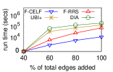
(a) Edge add., Digg (DWA)

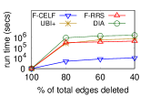
(b) Edge del., Slashdot (TV)

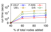
(c) Node add., Epinions (TV)

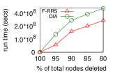
(d) Node del., Flickr (DWA)

Figure 4. Run time to adjust seed set, IC model, seed sets are adjusted after every update

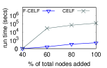
(a) Node add., Slashdot (DWA)

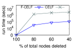
(b) Node del., Epinions (DWA)

Figure 5. Run time to adjust seed set, MIA model, seed sets are adjusted after every update

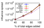
(a) Inf. spread, edge add.,
Digg (DWA) in IC model

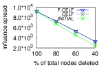
(b) Inf. spread, node del.,
Epinions (DWA) in MIA model

Figure 6. Influence spread, seed sets are adjusted after every update

$\bullet$ Influence strength models. We adopt two popular edge probability models for our experiments. Those are exactly the same models used by our competitors: UBI+ (Song et al., 2017) and DIA (Ohsaka et al., 2016). (1) Degree Weighted Activation (DWA) Model. In this model (Kempe et al., 2003; Ohsaka et al., 2016; Song et al., 2017) (also known as weighted cascade model), the influence strength of the edge $(uv)$ is equal to $1/d_{in}(v)$, where $d_{in}(v)$ is the in-degree of the target node $v$. (2) Trivalency (TV) Model. In this model (Kempe et al., 2003; Ohsaka et al., 2016), each edge is assigned with a probability, chosen uniformly at random, from $(0.1,0.01,0.001)$.

$\bullet$ Competing Algorithms. (1) FAMILY-CELF (F-CELF). This is an implementation of our proposed N-FAMILY framework, on top of the CELF influence maximization algorithm. (2) FAMILY-RR-Sketch (F-RRS). This is an implementation of our proposed N-FAMILY framework, on top of the RR-Sketch influence maximization algorithm. (3) DIA. The DIA algorithm was proposed in (Ohsaka et al., 2016), on top of the RR-Sketch. The method generates all RR-sketches only once; and after every update, quickly modifies those existing sketches. After that, all seed nodes are identified from ground using the modified sketches. This is the key difference with our algorithm F-RRS, since we generally need to identify only a limited number of new seed nodes, based on the affected region due to the update. (4) UBI+. The UBI+ algorithm (Song et al., 2017) performs greedy exchange for multiple times — every time an old seed node is replaced with the best possible non-seed node. If one continues such exchanges until there is no improvement, the method will guarantee 0.5-approximation. However, due to efficiency reasons, (Song et al., 2017) limits the number of exchanges to $k$, where $k$ is the cardinality of the seed set. An upper bounding method is used to find such best possible non-seed nodes at every round.

$\bullet$ Parameters Setup. (1) #Seed nodes. We varied seed set size from 5$\sim$100 (default 30 seed nodes). (2) #RR-Sketches. Our total number of sketches are roughly bounded by $\beta(|V|+|E|)\log|V|$ as given in (Ohsaka et al., 2016), and we varied $\beta$ from 2$\sim$512 (default $\beta=2^{5}=32$ (Ohsaka et al., 2016)). (3) Size of family. The family size $|F_{1}(u)|$ of a node $u$ is decided by the parameter $\theta$, and we varied $\theta$ from 1$\sim$0.01 (default $\theta$=0.1). (4) #IR to compute TIR. We consider upto 3-IR to compute TIR (default upto 2-IR). (5) Influence diffusion models. We employ IC (Kempe et al., 2003) and MIA (Chen et al., 2010) models for influence cascade. Bulk of our empirical results are provided with the IC model, since this is widely-used in the literature. (6) #MC samples. We use MC simulation 10 000 times to compute the influence spread in IC model (Kempe et al., 2003).

The code is implemented in Python, and the experiments are performed on a single core of a 256GB, 2.40GHz Xeon server. All results are averaged over 10 runs.

6.2. Single Update Results

First, we show results for single update queries related to edge addition, edge deletion, node addition, and node deletion. We note that adding an edge $uv$ can also be considered as an increase in the edge probability from $0$ to $P_{e}(uv)$. Analogously, deleting an edge can be regarded as a decrease in edge probability. Moreover, for the DWA edge influence model, when an edge is added or deleted, the probabilities of multiple adjacent edges are updated (since, inversely proportional to node degree). (1) Edge addition. We start with initial 40% of the edges in the graph data, and then add all the remaining edges as dynamic updates. We demonstrate our results with the Digg dataset and the DWA edge influence model (Figure 4(a)). (2) Edge deletion. We delete the last 60% of edges from the graph as update operations. We use the Slashdot dataset, with TV model, for showing our results (Figure 4(b)). (3) Node addition. We start with the first $40$% of nodes and all their edges in the dataset. We next added the remaining nodes sequentially, along with their associated edges. We present our results over Epinions, along with the TV model (Figure 4(c)). (4) Node deletion. We delete the last $20$% of nodes, with all their edges from the graph. We use our largest dataset Flickr and the DWA model for demonstration (Figure 4(d)).

For the aforesaid operations, we adjust the seed set after every update, since one does not know apriori when the seed set actually changes, and hence, it can be learnt only after updating them.

Efficiency. In Figure 4, we present the running time to dynamically adjust the top-$k$ seed nodes, under the IC influence cascade model. We find that F-CELF and F-RRS are always faster than UBI+ and DIA, respectively, by 1$\sim$2 orders of magnitude. As an example, for node addition over Epinions in Figure 4(c), the time taken by F-CELF is only $2\times 10^{6}$ sec for about $80$K node additions (i.e., 24.58 sec/node add). In comparison, UBI+ takes around $8\times 10^{7}$ sec (i.e., 1111.21 sec/ node add). Our F-RRS algorithm requires about $4\times 10^{5}$ secs (i.e., 5.31 sec/ node add), and DIA takes $10\times 10^{6}$ sec (i.e., 134.68 sec/node add). These results clearly demonstrate the efficiency improvements by our methods.

We also note that sketch-based methods are relatively slower (i.e., F-RRS vs. F-CELF, and DIA vs. UBI+) in smaller graphs (e.g., Digg and Slashdot). This is due to the overhead of updating sketches after graph updates. On the contrary, in our larger datasets, Epinions and Flickr, the benefit of sketches is more evident as opposed to MC-simulation based techniques. In fact, both F-CELF and UBI+ are very slow for our largest Flickr dataset (see Table 1); hence, we only show F-RRS and DIA for Flickr in Figure 4(d).

Additionally, in Figure 5, we show the efficiency of our method under the MIA model of influence spread. Since it is non-trivial to adapt UBI+ and DIA for the MIA model, we compare our algorithm F-CELF with CELF (Leskovec et al., 2007) in these experiments. For demonstration, we consider Slashdot and Epinions, together with node addition and deletion, respectively. It can be observed from Figure 5 that F-CELF is about 2 orders of magnitude faster than CELF. These results illustrate the generality and effectiveness of our approach under difference influence cascading models.

Table 4. Memory consumed by different algorithms

Algorithms	Digg	Slashdot	Epinions	Flickr
F-CELF, UBI+	0.22 GB	0.32 GB	1.03 GB	31.55 GB
F-RRS, DIA	3.83 GB	5.89 GB	25.87 GB	142.89 GB

Influence spread. We report the influence spread with the updated seed set for both IC (Figure 6(a)) and MIA models (Figure 6(b)). It can be observed that the competing algorithms, i.e., F-CELF, F-RRS, UBI+, and DIA achieve similar influence spreads with their updated seed nodes. Furthermore, we also show by INITIAL the influence spread obtained by the old seed set in the modified graph. We find that INITIAL achieves significantly less influence spread, especially with more graph updates. These results demonstrate the usefulness of dynamic IM techniques in general, and also the effectiveness of our algorithm in terms of influence coverage.

Memory usage. We show the memory used by all algorithms in Table 4. We find that MC-sampling based algorithms (i.e., F-CELF and UBI+) take similar amount of memory, whereas sketch-based techniques (i.e., F-RRS and DIA) also have comparable memory usage. Our results illustrate that the proposed methods, F-CELF and F-RRS improve the updating time of the top-$k$ influencers by 1$\sim$2 orders of magnitude, compared to state-of-the-art algorithms, while ensuring similar memory usage and influence spreads.

6.3. Batch Update Results

We demonstrate batch updates with a sliding window model as used in (Song et al., 2017). In this model, initially we consider the edges present in between $0$ to $W$ units of time (length of window) and compute the seed set. Next, we slide the window to $L$ units of time. The edges present in between $L$ and $W+L$ are considered as the updated data, and our goal is to adjust the seed set based on the updated data. We delete the edges from $0$ to $L$ and add the edges from $W$ to $W+L$. We continue sliding the window until we complete the whole data.

We conducted this experiment using the Twitter dataset downloaded from https://snap.stanford.edu/data/. The dataset is extracted from the tweets posted between 01-JUL-2012 to 07-JUL-2012, which is during the announcement of the Higgs-Boson particle. This dataset contains $304\,199$ nodes and $555\,481$ edges. Probability of an edge $uv$ is given by the formula $1-e^{\frac{-f}{k}}$, where $f$ is the total number of edges appeared in the window, and $k$ is the constant. We present our experimental results by varying $W$ from 30 mins to 6 hrs and $L$ from 1 sec to 2 mins. We set the value of $k$ as $5$. On an average, $1.8$ updates appear per second. Since the number of edges in a window is small, we avoid showing results with F-RRS. This is because F-CELF performs much better on smaller datasets. From the experimental results in Figure 7, we find that F-CELF is faster than both UBI+ and DIA upto three orders of magnitude.

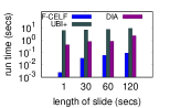
(a) Run time to adjust seed set, varying $L$, $W$ = 1 hour

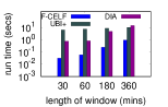
(b) Run time to adjust seed set, varying $W$, $L$ = 60 secs

Figure 7. Impacts of varying batch sizes, sliding window model, Twitter, IC influence prop., seed sets are adjusted after every slide

6.4. Sensitivity Analysis

In these experiments, we vary the parameters of our algorithms. For demonstration, we update the last 40$\%$ nodes in a dataset, and report the average time taken to re-adjust the seed set per update operation, with the F-RRS algorithm.

With increase in the size of TIR, number of seed nodes that get infected may increase. For a given update, size of TIR depends of two factors: $\theta$ (with decrease in $\theta$, size of family increases: Figure 8(c)) and $\#{\sf IR}$ to compute TIR. Hence, we vary $\theta$ (Figure 8) and $\#{\sf IR}$s (Figure 9) for node deletion in Epinions. We find that by selecting $\theta=10^{-1}$, influence spread increases by around $8.4$% compared to that of $\theta=10^{0}$, and there is no significant increase in influence spread for even smaller $\theta$. Similarly, for increase in $\#{\sf IR}$ almost saturates at $\#$IR=$2$. However, the efficiency of the algorithm decreases almost linearly with decrease in $\theta$ (Figure 8(b)) and increase in $\#{\sf IR}$s. Hence, by considering a trade off between efficiency and influence coverage we select $\theta=10^{-1}$ and $\#$2-IR to to compute TIR.

(a) Inf. Spread

(b) Run time to adjust seeds

(c) Avg. family size w/ $\theta$

Figure 8. Impacts of $\theta$, node del., Epinions (DWA), IC model

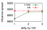
(a) Inf. spread

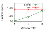
(b) Run time to adjust seed set

Figure 9. Impacts of #IRs, node del., Epinions (DWA), IC model

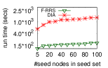
(a) Run time to adjust seeds, node add., Epinions

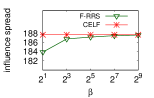
(b) Inf. spread w/ varying $\beta$,
Digg

Figure 10. Impacts of varying #seeds and $\beta$, IC model

In Figure 10(a), we show the efficiency with varying seed set size from $5$ to $100$. It can be observed that even for the seed set of size $100$, F-RRS is faster than DIA by more than an order of magnitude. This demonstrates that our technique is scalable for large seed set sizes. For sketch-based methods, choosing the optimal $\beta$ is very important. In Figure 10(b), we show the influence coverage of the F-RRS with varying $\beta$ from $2$ to $512$. We compare the influence spread with that of CELF. We find that with increase in $\beta$, influence coverage initially increases, and gets saturated at $\beta=32$. Hence, we set $\beta=32$ in our experiments.

7. Conclusions

We developed a generalized, local updating framework for efficiently adjusting the top-$k$ influencers in an evolving network. Our method iteratively identifies only the affected seed nodes due to dynamic updates in the influence graph, and then replaces them with more suitable ones. Our solution can be applied to a variety of information propagation models and influence maximization techniques. Our algorithm, N-Family ensures $(1-\frac{1}{e})$ approximation guarantee with the MIA influence cascade model, and works well for localized batch updates. Based on a detailed empirical analysis over several real-world, dynamic, and large-scale networks, N-Family improves the updating time of the top-$k$ influencers by 1$\sim$2 orders of magnitude, compared to state-of-the-art algorithms, while ensuring similar memory usage and influence spreads.

Appendix A Proof of Lemma 3

According to Eq. 2, the marginal gain of $u$ with respect to $S$ is given as:

$$MG(S,u) =\sigma{(S\cup\{u\})}-\sigma{(S)}$$

$$=\sum_{w\in V}{pp(S\cup\{u\},w)}-\sum_{w\in V}{pp(S,w)}$$

$$=\sum_{w\in V\setminus F_{1}(s)}{pp(S\cup\{u\},w)}+\sum_{w\in F_{1}(s)}{pp(S\cup\{u\},w)}-$$

(16) $$\sum_{w\in V\setminus F_{1}(s)}{pp(S,w)}-\sum_{w\in F_{1}(s)}{pp(S,w)}$$

As $u\notin F_{2}(s)$, the influence of $u$ on any node in $F_{1}(s)$ is $0$. Hence, Equation 16 can be written as:

$$MG(S,u) =\sum_{w\in V\setminus F_{1}(s)}{pp(S\cup\{u\},w)}+\sum_{w\in F_{1}(s)}{pp(S,w)}-$$

$$\sum_{w\in V\setminus F_{1}(s)}{pp(S,w)}-\sum_{w\in F_{1}(s)}{pp(S,w)}$$

(17) $$=\sum_{w\in V\setminus F_{1}(s)}{pp(S\cup\{u\},w)}-\sum_{w\in V\setminus F_{1}(s)}{pp(S,w)}$$

Now, the removed seed node $s$ cannot influence any node outside $F_{1}(s)$. Hence, Equation 17 can be written as:

$$MG(S,u) =\sum_{w\in V\setminus F_{1}(s)}{pp({S\setminus\{s\}}\cup\{u\},w)}-\sum_{w\in V\setminus F_{1}(s)}{pp({S\setminus\{s\}},w)}$$

$$=\sum_{w\in V\setminus F_{1}(s)}{pp({S\setminus\{s\}}\cup\{u\},w)}+\sum_{w\in F_{1}(s)}{pp({S\setminus\{s\}}\cup\{u\},w)}$$

(18) $$-\sum_{w\in V\setminus F_{1}(s)}{pp({S\setminus\{s\}},w)}-\sum_{w\in F_{1}(s)}{pp({S\setminus\{s\}}\cup\{u\},w)}$$

As influence of $u$ on any node in $F_{1}(s)$ is $0$, Equation 18 can be written as:

$$MG(S,u) =\sum_{w\in V\setminus F_{1}(s)}{pp({S\setminus\{s\}}\cup\{u\},w)}+\sum_{w\in F_{1}(s)}{pp({S\setminus\{s\}}\cup\{u\},w)}$$

$$-\sum_{w\in V\setminus F_{1}(s)}{pp({S\setminus\{s\}},w)}-\sum_{w\in F_{1}(s)}{pp({S\setminus\{s\}},w)}$$

$$=\sum_{w\in V}{pp({S\setminus\{s\}}\cup\{u\},w)}-\sum_{w\in V}{pp({S\setminus\{s\}},w)}$$

$$=\sigma{({S\setminus\{s\}}\cup\{u\})}-\sigma{(S\setminus\{s\})}$$

(19) $$=MG(S\setminus\{s\},u)$$

Hence, the lemma.

Appendix B Proof of Lemma 4

Consider a node $w$ outside $MIIA(u,\theta)$ in the original graph $\mathcal{G}(V,E,P)$, which means $w$ cannot activate $u$ with a minimum strength of $\theta$ through $MIP(w,u)$. Then, the strength at which $w$ activates $v$ through $u$ in the updated graph is: $pp(w,u)\times P_{u,v}$. Since, $pp(w,u)<\theta$, we have: $pp(w,u)\times P_{u,v}<\theta$. Thus, adding the edge $uv$ does not change the expected influence spread of $w$, based on the MIA model. Hence, the lemma follows.

Appendix C Proof of Lemma 5 and 6

A seed node can influence only the nodes present in its family according to the MIA model. There is no node present in TIR which belongs to the family of any seed node outside TIR. This is because any uninfected seed node is more than 2-Family away from any node present in TIR (This is how we terminate infection propagation). Hence, both Lemma 5 and 6 follow.

Appendix D Proof of Performance
Guarantee under MIA Model

We show that the top-$k$ seed nodes reported by our N-Family method (Algorithm 2) are the same as the top-$k$ seed nodes obtained by running the Greedy on the updated graph under the MIA model. Since, the Greedy algorithm provides the approximation guarantee of $1-\frac{1}{e}$, our N-Family also provides the same approximation guarantee. The proof is as follows.

As described in Section 4.2.1, after identifying the TIR using Equation 12, we compute $S_{rem}$ (=$S\setminus{\sf TIR}$), influence spreads of all nodes $u\in{\sf TIR}$, and update the priority queue.

Now, we continue with computing the $k-k^{\prime}$ new seed nodes over the updated graph, and $S_{new}$ is new seed set (of size $k$) found in this manner. Note that before we begin computing new seed nodes, $S_{new}$ contains the $k^{\prime}$ seed nodes present in $S_{rem}$, and then new nodes are added in an iterative manner. Clearly, $S_{new}^{k^{\prime}}$ is same as $S_{rem}$. We consider $s_{n}^{k^{\prime}+i}$ as the seed node computed by Greedy in the $i^{th}$ iteration, where $i\leq k-k^{\prime}$. Due to Greedy algorithm,

(20) $$MG(S_{new}^{k-1},s_{n}^{k})\geq MG(S_{new}^{k-1},u),\qquad\forall u\in V\setminus S_{new}$$

Next, we sort all seeds in $S_{new}$ according to the greedy inclusion order, and the sorted seed set is denoted as $S_{order}$. Note that seed nodes present in $S_{new}$ and $S_{order}$ are same, but their order could be different. At this stage, the important observations are as follows.

After computing $S_{order}$, and assuming $w$ the top-most node in the priority queue, we will have two mutually exclusive cases:

Case 1: $MG(S_{order}^{k-1},s_{o}^{k})\geq MG(S_{order},w)$
Case 2: $MG(S_{order}^{k-1},s_{o}^{k})<MG(S_{order},w)$

If we end up with Case-1, we terminate our algorithm and report $S_{order}$ as the set of new seed nodes, which would be same as the ones computed by the Greedy algorithm on the updated graph (we shall prove this soon). However, if we arrive at Case-2, we do iterative seed replacements until we achieve Case-1 (we prove that by iterative seed replacements for at most $k^{\prime}$ times, we reach Case-1).

Moreover, there are two more mutually exclusive cases which can be derived from the following lemma.

Lemma 7.

The last seed node, $s_{o}^{k}$ present in $S_{order}$ can be either $s_{r}^{k^{\prime}}$ (i.e., the last seed node in $S_{rem}$) or $s_{n}^{k}$ (i.e., the last seed node in $S_{new}$).

Proof.

Since we compute new seed nodes using Greedy algorithm for $S_{new}$, $MG(S_{new}^{k-1},s_{n}^{k})\leq MG(S_{new}^{k^{\prime}+i-1},s_{n}^{k^{\prime}+i})$ for $0<i\leq(k-k^{\prime})$ (Inequality 3), and $MG(S_{rem}^{k^{\prime}-1},s_{r}^{k^{\prime}})\leq MG(S_{rem}^{k^{\prime}-l},s_{r}^{k^{\prime}-l+1})$ (Inequality 13) where $2\leq l\leq k^{\prime}$. In other words, $s_{r}^{k^{\prime}}$ and $s_{n}^{k}$ provide least marginal gains compared to other nodes in $S_{rem}$ and in $S_{new}/S_{rem}$, respectively. Hence, $s_{o}^{k}$ can be either $s_{n}^{k}$ or $s_{r}^{k^{\prime}}$. ∎

Therefore, the two mutually exclusive cases are:

Case A: $s_{o}^{k}=s_{n}^{k}$ (i.e., the last seed node in $S_{new}$)
Case B: $s_{o}^{k}=s_{r}^{k^{\prime}}$ (i.e., the last seed node in $S_{rem}$)

Now, we will show that the seed nodes obtained after reaching Case-1, i.e., when $MG(S_{order}^{k-1},s_{o}^{k})\geq MG(S_{order},w)$, and under both Case-A and Case-B, i.e., $s_{o}^{k}=s_{n}^{k}$ and $s_{o}^{k}=s_{r}^{k^{\prime}}$, are exactly same as the seed nodes produced by Greedy algorithm on the updated graph. For the seed set computed by the Greedy algorithm on the updated graph, the following inequality must hold.

(21) $$MG(S_{order}^{k-1},s_{o}^{k})\geq MG(S_{order}^{k-1},v),\qquad\forall v\in V\setminus S_{order}$$

Hence, we will prove that for Case-1, Inequality 21 is true in both Case-A and Case-B.

First, we will show for Case-1 ($MG(S_{order}^{k-1},s_{o}^{k})\geq MG(S_{order},w)$) and Case-A ($s_{o}^{k}=s_{n}^{k})$.

Lemma 8.

If $MG(S_{order}^{k-1},s_{o}^{k})\geq MG(S_{order},w)$ (Case-1), where $w$ is the top-most node in the priority queue, and $s_{o}^{k}=s_{n}^{k}$ (Case-A), then $S_{order}$ is the set of seed nodes computed by Greedy on the updated graph, i.e., Inequality 21 holds.

Proof.

Given $s_{o}^{k}=s_{n}^{k}$. Moreover, seed nodes present in $S_{order}$ and $S_{new}$ are same. Hence,

(22) $$MG(S_{order}^{k-1},s_{o}^{k})=MG(S_{new}^{k-1},s_{n}^{k})$$

Next, by combining Equation 22 and Inequality 20 we get, $MG(S_{order}^{k-1}$ $,s_{o}^{k})\geq MG(S_{order}^{k-1},u)$, for all $u\in V\setminus S_{order}$. Hence, the lemma. ∎

Now, to prove the theoretical guarantee for Case-1 and Case-B, the following Lemma is very important.

Lemma 9.

If $s_{o}^{k}=s_{r}^{k^{\prime}}$, then

1. All new seed nodes computed belong to TIR, i.e.,
   $S_{order}\setminus S_{rem}\in\text{\sf TIR}$.

2. $MG(S_{order}^{k-1},s_{o}^{k})=MG(S_{rem}^{k^{\prime}-1},s_{r}^{k^{\prime}})$.

Proof.

As $s_{r}^{k^{\prime}}$ provides the least marginal gain in $S_{order}$, according to Inequality 14, any other node in $V\setminus\{{\sf TIR\cup S_{rem}}\}$ cannot be present in $S_{order}\setminus S_{rem}$. Hence, all new seed nodes come from TIR. This completes the proof of the first part.

The second part of the theorem also holds, since the new seed nodes (i.e., $S_{order}\setminus S_{rem}$) present in TIR do not affect the marginal gain of the old seed nodes (i.e., $S_{rem}$) outside TIR. It is because they are at least 2-Family away from old seed nodes (Lemma 3). ∎

Now, we are ready to prove that Inequality 21 holds for Case-1 (i.e., $MG(S_{order}^{k-1},s_{o}^{k})\geq MG(S_{order},w)$) and Case-B (i.e., $s_{o}^{k}=s_{r}^{k^{\prime}}$).

Lemma 10.

If $MG(S_{order}^{k-1},s_{o}^{k})\geq MG(S_{order},w)$ (Case-1) where $w$ is the top-most node in the priority queue, and $s_{o}^{k}=s_{r}^{k^{\prime}}$ (Case-B) then $S_{order}$ is the set of seed nodes computed by Greedy on the updated graph, i.e., Inequality 21 holds.

Proof.

We prove this lemma for the nodes present in TIR and outside TIR separately.

First, we will prove that the lemma is true for $u\in V\setminus\{{\sf TIR}\cup S_{order}\}$. As $S_{rem}^{k^{\prime}-1}\subseteq S_{order}^{k-1}$, due to Lemma 1 (i.e., sub-modularity):

(23) $$MG(S_{rem}^{k^{\prime}-1},u)\geq MG(S_{order}^{k-1},u),\quad\forall u\in V\setminus\{{\sf TIR}\cup S_{order}\}$$

When $s_{o}^{k}=s_{r}^{k^{\prime}}$, $S_{order}\setminus S_{rem}\in{\sf TIR}$ (Lemma 9.1). Hence, $TIR\cup S_{order}=TIR\cup S_{rem}$. From Inequality 14,

(24) $$MG(S_{rem}^{k^{\prime}-1},s_{r}^{k^{\prime}})\geq MG(S_{rem}^{k^{\prime}-1},u),\quad\forall u\in V\setminus\{{\sf TIR}\cup S_{order}\}$$

By combining Lemma 9.2, Inequality 23, and Inequality 24, we get $MG(S_{order}^{k-1},s_{o}^{k})\geq MG(S_{order}^{k-1},u)$, for all $u\in V\setminus\{\text{\sf TIR}\cup S_{order}\}$.

Now, what is left to be proved is that Inequality 21 holds for all nodes $u\in\text{\sf TIR}\setminus S_{order}$. As every such node $u$ is at least 2-Family away from $s_{r}^{k^{\prime}}$, according to Lemma 3,

(25) $$MG(S_{order}^{k-1},u)=MG(S_{order}^{k},u),\quad\forall u\in\text{\sf TIR}\setminus S_{order}$$

Since $w$ is the top-most node in the priority queue, and our assumption is that $MG(S_{order}^{k-1},s_{o}^{k})\geq MG(S_{order},w)$, then

$$MG(S_{order}^{k-1},s_{o}^{k})\geq MG(S_{order},w) \geq MG(S_{order},u)$$

(26) $$=MG(S_{order}^{k-1},u)$$

From the Inequality 26, we get $MG(S_{order}^{k-1},s_{o}^{k})\geq MG(S_{order}^{k-1},u)$ for all nodes $u\in\text{\sf TIR}\setminus S_{order}$. This completes the proof. ∎

Now, we show that for Case-2, i.e., $MG(S_{order}^{k-1},s_{o}^{k})$ $<MG(S_{order},$ $w)$, where $w$ is the top node in the priority queue, by doing iterative seed replacement for a maximum of $k^{\prime}$ times, we achieve Case-1. Hence, our N-Family method provides the seed set same as the one provided by Greedy on the updated graph. First, we prove that for Case-2, only Case-B (i.e., $s_{o}^{k}$ = $s_{r}^{k^{\prime}}$) holds, and $w\in{\sf TIR}\setminus S_{order}$.

Lemma 11.

Consider $w$ as the top-most node in the priority queue, and $MG(S_{order}^{k-1},s_{o}^{k})<MG(S_{order},w)$ (Case-2). Then,
1. $s_{o}^{k}=s_{r}^{k^{\prime}}$ (Case-A)
2. $w\in TIR\setminus S_{order}$

Proof.

We prove both parts of this lemma by contradiction.

For the first part, let us assume $s_{o}^{k}\neq s_{r}^{k^{\prime}}$, which means $s_{o}^{k}=s_{n}^{k}$(Case-B). For all nodes $u\in V\setminus{S_{new}}$,

From Lemma 1, we get:

(27) $$MG(S_{new}^{k-1},u)\geq MG(S_{new},u).$$

Since $S_{new}=S_{order}$, and by combining Inequality 20 and Inequality 27, we get $MG(S_{order}^{k-1},s_{o}^{k})\geq MG(S_{order},u)$. This contradicts the given condition. Hence, $s_{o}^{k}=s_{r}^{k}$.

For the second part of the lemma, let us assume that $w\in V\setminus\{{\sf TIR}\cup S_{order}\}$ (obviously, $w\notin S_{order}$). From the first part of the lemma, we have $s_{o}^{k}=s_{r}^{k^{\prime}}$.

Since $S_{order}\setminus S_{rem}\in{\sf TIR}$, ${\sf TIR}\cup S_{order}={\sf TIR}\cup S_{rem}$. From Inequality 14, for $w\in V\setminus{TIR\cup S_{order}}$, we get:

(28) $$MG(S_{rem}^{k^{\prime}-1},s_{r}^{k^{\prime}})\geq MG(S_{rem}^{k^{\prime}-1},w)$$

Since $S_{rem}^{k-1}\subset S_{order}$, from Lemma 1, we have:

(29) $$MG(S_{rem}^{k^{\prime}-1},w)\geq MG(S_{order},w)$$

Following Lemma 9.2, Inequality 28 and Inequality 29, we get that $MG(S_{order}^{k-1},s_{o}^{k})\geq MG(S_{order},w)$, which contradicts our assumption. Hence, $w\in TIR\setminus S_{order}$. This completes the proof. ∎

Now, in our iterative seed replacement phase, we begin with removing $s_{o}^{k}$ ($=s_{r}^{k^{\prime}}$) from $S_{order}$; for every node $u\in F_{2}(s_{o}^{k})\setminus S_{order}$, compute the marginal gain $MG(S_{order}^{k-1},u)$, and update the priority queue. After updating the priority queue, we compute the new seed node from the updated graph by running Greedy over it. The new seed node computed comes from ${\sf TIR}\setminus S_{order}^{k-1}$, more specifically, it is the top-most node $w$ in the priority queue, as demonstrated below.

Lemma 12.

If $w$ is the top-most node in the priority queue and $MG(S_{order}^{k-1},s_{o}^{k})<MG(S_{order}\cup\{s_{o}^{k}\},w)$, then the new seed node that replaces $s_{o}^{k}$ ($=s_{r}^{k^{\prime}}$) is $w$. To prove the lemma, we prove that $MG(S_{order}^{k-1},w)\geq MG(S_{order}^{k-1},u)$ for all nodes $u\in V\setminus S_{order}^{k-1}$.

Proof.

From Lemma 11.1, $s_{o}^{k}=s_{r}^{k^{\prime}}$ and from Lemma 11.2, $w\in{\sf TIR}\setminus S_{order}$. We prove this lemma for the nodes present in TIR and outside TIR seperately.

First, we shall prove that $MG(S_{order}^{k-1},w)\geq MG(S_{order}^{k-1},u)$ holds for $u\in V\setminus\{TIR\cup S_{order}^{k-1}\}$. From Lemma 1 (i.e., sub-modularity), we get:

$$MG(S_{order}^{k-1},w) \geq MG(S_{order}^{k-1}\cup\{s_{o}^{k^{\prime}}\},w)$$

(30) $$>MG(S_{order}^{k-1},s_{o}^{k})\quad\text{(due to Case-2 condition)}$$

Combining Inequality 30, Lemma 9.2, and Inequality 14 we get:

(31) $$MG(S_{order}^{k-1},w)>MG(S_{rem}^{k^{\prime}-1},u)$$

According to Lemma 1 (submodularity), Inequality 31 can be written as $MG(S_{order}^{k-1},w)>MG(S_{order}^{k-1},u)$ for all nodes $u\in V\setminus\{TIR\cup S_{order}^{k-1}\}$.

What is left to be proved is that $MG(S_{order}^{k-1},w)\geq MG(S_{order}^{k-1},u)$ holds for all $u\in{\sf TIR}\setminus S_{order}^{k-1}$. Since $w$ is the top-most node in the priority queue, we get:

(32) $$MG(S_{order}^{k-1}\cup\{s_{r}^{k^{\prime}}\},w)\geq MG(S_{order}^{k-1}\cup\{s_{r}^{k^{\prime}}\},u)$$

Moreover, $u$ and $w$ are at least 2-Family away from $s_{r}^{k^{\prime}}$. Thus, according to Lemma 3, Inequality 32 can be written as

(33) $$MG(S_{order}^{k-1},w)\geq MG(S_{order}^{k-1},u)$$

This completes the proof. ∎

After computing the new seed node, we check if we arrived at Case-1. If so, we terminate the algorithm, and report $S_{order}$ as the set of new seed nodes. Otherwise, we execute this iterative process for maximum of $k^{\prime}$ times to reach Case-1. The following lemma ensures that the iterative seed replacement for a maximum of $k^{\prime}$ times leads us to Case-1.

Lemma 13.

Iterative seed replacement for a maximum of $k^{\prime}$ times leads us to Case-1, i.e., $MG(S_{order}^{k-1},s_{o}^{k})\geq MG(S_{order},w)$, $w$ is the top-most node in the priority queue.

Proof.

According to Lemma 11.1, for Case-2, the seed node with the least marginal gain belongs to $S_{rem}$. Since $|S_{rem}|=k^{\prime}$, we can perform a maximum of $k^{\prime}$ replacements. Assume that we executed iterative seed replacement for $k^{\prime}-1$ times, and we are still at Case-2. According to Lemma 12, the new seed nodes computed for the past $k^{\prime}-1$ times came from TIR. At this stage, $s_{r}^{1}$ is the remaining old seed node outside TIR, and $S_{order}^{k-1}$ are the set of seed nodes inside TIR (Lemma 12). Let $x$ be the top-most node in the priority queue; hence, $x\in TIR\setminus S_{order}^{k-1}$ (Lemma 7.1), and $s_{o}^{k}=s_{r}^{1}$ (Lemma 7.2). According to Lemma 12, $x$ would be the new seed node. Hence, we shall prove that $MG(S_{order}^{k-1},x)\geq MG(S_{order}^{k-1}\cup\{x\},u)$, for all $u\in V\setminus S_{order}^{k-1}$. Since we prove for all nodes $u\in V\setminus S_{order}^{k-1}$, it is true for $w$ also. We will prove the lemma for the nodes present in TIR and outside TIR separately.

First, we will prove that $MG(S_{order}^{k-1},x)>MG(S_{order}^{k-1}\cup\{x\},u)$ for all nodes $u\in V\setminus TIR$. Since, $s_{r}^{1}$ is at least 2-Family away from $x$, according to Lemma 3 and our assumption that $x$ is the top-most node in the priority queue, we get:

(34) $$MG(S_{order}^{k-1},x)=MG(S_{order}^{k-1}\cup\{s_{r}^{1}\},x)>MG(S_{order}^{k-1},s_{r}^{1})$$

Since $\{S_{order}^{k-1}\cup\{{s_{r}^{1}}\}\}\setminus\{s_{r}^{1}\}\in{\sf TIR}$ (Lemma 9.1), $s_{r}^{1}$ is the only seed node outside TIR, and is at least 2-Family away from all seed nodes in TIR, the Inequality 35 can be written as

(35) $$MG(S_{order}^{k-1},x)>MG(S_{order}^{k-1},s_{r}^{1})=\sigma(s_{r}^{1})\geq\sigma(u)$$

Since the influence spread of a node is always greater than or equal to its marginal gain with respect to any seed set, Inequality 35 can be written as

(36) $$MG(S_{order}^{k-1},x)>MG(S_{order}^{k-1}\cup\{x\},u)$$

What is left to be proved is that $MG(S_{order}^{k-1},x)\geq MG(S_{order}^{k-1}\cup\{x\},u)$ for all nodes $u\in{\sf TIR}\setminus S_{order}^{k-1}$. According to our assumption that $x$ is the top-most node in the priority queue, we get:

(37) $$MG(S_{order}^{k-1}\cup\{s_{r}^{1}\},x)\geq MG(S_{order}^{k-1}\cup\{s_{r}^{1}\},u)$$

We also have $x\in{\sf TIR}\setminus\{S_{order}^{k-1}\}$ (Lemma 7.2). Moreover, $u$ and $x$ are at least 2-Family away from $s_{r}^{1}$. Following Lemma 3, the Inequality 37 can be written as

(38) $$MG(S_{order}^{k-1},x)\geq MG(S_{order}^{k-1},u)$$

On the other hand, from Lemma 1 (submodularity), we get:

(39) $$MG(S_{order}^{k-1},u)\geq MG(S_{order}^{k-1}\cup\{x\},u)$$

Following Inequality 38 and Inequality 39, we get: $MG(S_{order}^{k-1},x)>MG(S_{order}^{k-1}\cup\{x\},u)$, for all nodes $u\in{\sf TIR}\setminus S_{order}^{k-1}$.

After completing $k^{\prime}$ iterations, $S_{order}^{k-1}\cup\{x\}$ becomes $S_{order}$, $s_{o}^{k}=x$, and $MG(S_{order}^{k-1},x)\geq MG(S_{order},u)$ for all nodes $u\in V\setminus{S_{order}}^{k-1}$. Hence, $MG(S_{order}^{k-1},s_{o}^{k})>MG(S_{order},w)$, where $w$ is the top-most node in the priority queue. Hence, the lemma. ∎

Theorem 1.

The top-$k$ seed nodes reported by our N-Family method provides $(1-\frac{1}{e})$ approximation guarantee to the optimal solution, under the MIA model.

Proof.

The top-$k$ seed nodes reported by our N-Family method are the same as the top-$k$ seed nodes obtained by running the Greedy on the updated graph under the MIA model (by following Lemma 8 and Lemma 10). Since, the Greedy algorithm provides the approximation guarantee of $1-\frac{1}{e}$ under the MIA model (Chen et al., 2010), our N-Family also provides the same approximation guarantee. ∎

References

- (1)
- Aggarwal et al. (2012) C. Aggarwal, S. Lin, and P. S. Yu. 2012. On Influential Node Discovery in Dynamic Social Networks. In SDM.
- Aggarwal and Subbian (2014) C. Aggarwal and K. Subbian. 2014. Evolutionary Network Analysis: A Survey. ACM Comput. Surv. 47, 1 (2014), 10:1–10:36.
- Borgs et al. (2014) C. Borgs, M. Brautbar, J. Chayes, and B. Lucier. 2014. Maximizing Social Influence in Nearly Optimal Time. In SODA.
- Chen et al. (2013) W. Chen, L. V. S. Lakshmanan, and C. Castillo. 2013. Information and Influence Propagation in Social Networks. Morgan & Claypool Publishers.
- Chen et al. (2010) W. Chen, C. Wang, and Y. Wang. 2010. Scalable Influence Maximization for Prevalent Viral Marketing in Large-Scale Social Networks. In KDD.
- Kempe et al. (2003) D. Kempe, J. M. Kleinberg, and E. Tardos. 2003. Maximizing the Spread of Influence through a Social Network. In KDD.
- Leskovec et al. (2007) J. Leskovec, A. Krause, C. Guestrin, C. Faloutsos, J. VanBriesen, and N. Glance. 2007. Cost-effective Outbreak Detection in Networks. In KDD.
- Liu et al. (2017) X. Liu, X. Liao, S. Li, J. Zhang, L. Shao, C. Huang, and L. Xiao. 2017. On the Shoulders of Giants: Incremental Influence Maximization in Evolving Social Networks. Complexity (2017).
- Ohsaka et al. (2016) N. Ohsaka, T. Akiba, Y. Yoshida, and K.-I. Kawarabayashi. 2016. Dynamic Influence Analysis in Evolving Networks. In VLDB.
- Song et al. (2017) G. Song, Y. Li, X. Chen, X. He, and J. Tang. 2017. Influential Node Tracking on Dynamic Social Network: An Interchange Greedy Approach. IEEE Trans. Knowl. Data Eng. 29, 2 (2017), 359–372.
- Subbian et al. (2016) K. Subbian, C. Aggarwal, and J. Srivastava. 2016. Mining Influencers Using Information Flows in Social Streams. ACM Trans. Knowl. Discov. Data 10, 3 (2016), 26:1–26:28.
- Tang et al. (2015) Y. Tang, Y. Shi, and X. Xiao. 2015. Influence Maximization in Near-Linear Time: A Martingale Approach. In SIGMOD.
- Tang et al. (2014) Y. Tang, X. Xiao, and Y. Shi. 2014. Influence Maximization: Near-Optimal Time Complexity Meets Practical Efficiency. In SIGMOD.
- Wang et al. (2017) Y. Wang, Q. Fan, Y. Li, and K.-L. Tan. 2017. Real-Time Influence Maximization on Dynamic Social Streams. In VLDB.
- Yang et al. (2017) Y. Yang, Z. Wang, J. Pei, and E. Chen. 2017. Tracking Influential Nodes in Dynamic Networks. IEEE Trans. Knowl. Data Eng. 29, 11 (2017), 2615–2628.
- Zhuang et al. (2013) H. Zhuang, Y. Sun, J. Tang, J. Zhang, and X. Sun. 2013. Influence Maximization in Dynamic Social Networks. In ICDM.