Detecting Zones and Threat on 3D Body for Security in Airports using Deep Machine Learning

Abstract

In this research, it was used a segmentation and classification method to identify threat recognition in human scanner images of airport security. The Department of Homeland Security’s (DHS) in USA has a higher false alarm, produced from theirs algorithms using today’s scanners at the airports. To repair this problem they started a new competition at Kaggle site asking the science community to improve their detection with new algorithms. The dataset used in this research comes from DHS at https://www.kaggle.com/c/passenger-screening-algorithm-challenge/data. According to DHS: "This dataset contains a large number of body scans acquired by a new generation of millimeter wave scanner called the High Definition-Advanced Imaging Technology (HD-AIT) system. They are comprised of volunteers wearing different clothing types (from light summer clothes to heavy winter clothes), different body mass indices, different genders, different numbers of threats, and different types of threats". Using Python as a principal language, the preprocessed of the dataset images extracted features from 200 bodies using: intensity, intensity differences and local neighbourhood to detect, to produce segmentation regions and label those regions to be used as a truth in a training and test dataset. The regions are subsequently give to a CNN deep learning classifier to predict 17 classes (that represents the body zones): zone1, zone2, … zone17 and zones with threat in a total of 34 zones. The analysis showed the results of the classifier an accuracy of 98.2863% and a loss of 0.091319, as well as an average of 100% for recall and precision.
Keywords—Deep learning; DHS; Security;

I Introduction

To be able to accurately identify objects camouflaged in the human body through artificial intelligence is one of the big challenge facing security today. There is, nowadays, a worldwide warning regarding airport security. This happen because of the terrorism that threatens the population or the great flow of foreigners that has been growing year by year. New systems, programs and intelligence of protection were created to help the teams that do security in the airports. According to Bart Elias [1], Transportation Security Administration (TSA) has deployed 1,800 units Advanced Image Technology (AIT) throughout the airports on USA and the acquisition cost per unit is about $175,000. To fully implement this system, the overall annual cost for purchasing, installing, staffing, operating, supporting, upgrading and maintaining sum to about 1.17 billion. Adding on it the Department of Homeland Security’s (DHS) in USA has a higher false alarm, produced from their algorithms using today’s scanners at the airports. Although, the investment being made represents a significant amount of money, it is not solving the security problem with regarding to the detection of threats. The Security still needs to develop technology to fix these algorithms to minimize the errors. Like others cleaners of data, working with images need a special care in filter data that should be a ground truth as possible. Peter Corke [2], discussed the difficulties in filter the noise in the images and in segmenting the images in regions that contains the object. Errors in the segmentation can mislead the security system. The ideal is to reduce the noise and produce some threshold that correct the segmentation regions. Considering this scenario, this paper work will present a model to do the classification of the regions of the body´s images using supervised machine learning to identify the threats hired in the bodies. The results will be analyzed to verify the true or false of the information collected in the model. The objectives proposed in this research are: Produce an algorithm that fractionated the human body image in regions to be able to identify the body’s region correctly. Use a supervised classification to recognize the human body’s regions. Use the training and test dataset to identify the true or false of the detection, for measuring their accuracy, recall and precision. Propose improvements in the algorithm for implementation.

II Previous Work and Literature

Bart Elias [1] described how Transport Security Administration (TSA) implement the new AIT units, using new millimeter wave images, that’s substitute the X-ray backscatter units, exposing the difference between those units and the risk of both systems in terms of health concern. It explains and describe Automated Target Recognition (ATR), also the scanners effectiveness measure regarding accuracy and the trade-off between detection and false alarm. David Powers [3] evaluated measures including Recall, Precision, F-Measure, Rand Accuracy and how the biases transform the concepts of the results, demonstrating the elegant connection of Informedness, Markedness, Correlation and Significance, as well providing their intuitive relationships with Recall and Precision. Sauvola [4] demonstrated a method of binary image with local and multiple threshold evaluation, instead of a global threshold. Those measures used formulas that take the window that surround of every pixel to take the threshold based on mean and standard deviation of the local neighborhood. Using a Hybrid switch technique, one method is based on histogram and other based on Soft decision (SDM), to produce a threshold using interpolation for a better result. Robinson [5] used a morphological reconstruction by dilation, that is different from the basic morphological dilation, where high-intensity values are replaced by nearby low-intensity values. In contrast, it uses two images, one image called “seed”, that specifies how far values can be spread, and a “mask” image, which allow each pixel to have a maximum value limiting the spread of high-intensity values. In his book, Peter [2] discussed about many techniques of image process Like monodic function (normalization, threshold, gamma), diadic functions (temporal smoothing), spatial (morphological), features (histograms), shape change (rotation, pyramid scale, ROI) among others. The language and the explanation that were used in this book facilitated the understanding. In this article, Sarraf and Tofighi [6] exposed a CNN deep learning data model using fMRI images to identify regions that has a pattern of Alzheimer’s Disease. It explained how the convolution and pull data work in the process of images, in which is obtained a classification. In addition, they showed the result using Receiver Operating Characteristics (ROC) curve, taking about 96.86% of the accuracy. Alex Krizhevsky [7] used a neural network with 60 million parameters and 650,000 neurons, their method consists of five convolution layers followed by max-pooling using a final 1000-way softmax. To make training faster, they used non-saturating neurons and a very efficient GPU implementation of the convolution operation. To reduce overfitting in the fully-connected layers was used a regularization method called “dropout”. LeCun [8][9] introduced the gradient-based learning for document recognition. It explained most of all techniques in Neural Network principally CNN, that imposed convolution learning in the layer steps, in that way it has invariance of shift, scale and distortion. Leon Bottou [10], strongly advocates to use the stochastic back-propagation method to train neural networks. It explains why SGD is a good learning algorithm to train large datasets. Those recommendations collaborated with this research. Bengio [11] prepared a practical guide recommendation to adjust common many hyper-parameters, based on back-propagated gradient, as well did questions about training difficulties observed in deep machine learning. Kumar [12] showed the basic ideas of how CNN was improved when it implements the interface with GPU. TensorFlow [13] is a model that represents and uses nodes as a data-flow graph, those nodes operates individual mathematical such as matrix multiplication, convolution, min and max and many more. With this approach user can compose layers using a high-level scripting or in a graph interface. Caffe [14] like TensorFlow, it is an open-source framework to access deep architectures. It uses CUDA for GPU computation that is implemented with C++, it can use to do an interface with Python/Numpy and Matlab. It is possible to process over 40 million images a day on a single K40 or Titan GPU ($\approx$ 2.5 ms per image). It also separates model network from actual implementation. Bishop [15] presented in his book most of all techniques to learn pattern recognition, it goes to the basic probability showing all principal model like regression, svn and others. It’s a good book to understand about pattern recognition and machine learning in all aspects. In his article, Davis [16] explained about both ROC curves and Recall Precision Graphs model, moreover he showed the difference between classes comparison. When its comparing two classes in the graph, class one showed a better result in ROC curve, than the class two; when change the graph for PR, class two has better result. In the Python world, Wall [17] developed the NumPy arrays. NumPy arrays are the standard representation for numerical data according to the community. Numpy arrays can implement efficient numerical computations for a high-level compute language using Python. There are three techniques that improve performance: vectorizing calculations, avoiding copying data in memory, and minimizing operation counts.

III Methodology

III-A Dataset

The dataset used in this research comes from DHS and Kaggle competition at: https://www.kaggle.com/c/passenger-screening-algorithm- challenge/data/ . According to DHS: “This dataset contains a large number of body scans acquired by a new generation of millimeter wave scanner called the High Definition-Advanced Imaging Technology (HD-AIT) system. They are comprised of volunteers wearing different clothing types (from light summer clothes to heavy winter clothes), different body mass indices, different genders, different numbers of threats, and different types of threats”. It will start with a small sample of the body’s scanned separating the data into two parts, to be used as a training set and testing set. After that, we can use more samples of the huge database to get better accuracy. For the stage1 of Kaggle Competition we have a total of 929 bodies with threat to be analyzed. Here, in this research, we will limit for a sample of 200 bodies to be analyzed; It will produce a total of 287660 sliced images of the bodies.

III-B Approach

Here is the block diagram of this paper. It tries to summarize all the steps needed to describe the algorithms in every step, those algorithms are writing using python language. A first approach is to divide the bodies in 17 regions that can contain threat or cannot contains threats.

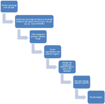
Figure 1: Approach block diagram

III-B1 Pull the raw image from 3D data

This step loads the data files, the 200 bodies from TSA database, in a extension of a3d file. The scanned body’s will be loaded one by one to produce labels regions. Each scanned sliced view has the length of the body through a z axis coordinate. Besides, TSA produces more 3 types of file scanned body: one that is scanned rotated around the z axis and saved with the extension aps; second in a mixed of ad3 and aps and; the last one is a high resolution of the body. In this research was used both the aps and a3d. The file a3d can be worked with the sliced plane (x, y) image of the body and the aps file, it was used to locate the threat’s body.

III-B2 Select from the image 3D where is the threat located in the body, in terms of ([x1, x2], [y1, y2], [z1, z2]) coordinates

This step pulls the threats from the dataset TSA that uses the file with extension aps. Every body will be rotated to localize the threat to pull the coordinates of the threat. Those coordinates will be saved in a table with the extension of csv file (table 1). An algorithm from Kaggle was modified to plot the bodies in a grid to determine the threat coordinates (x, y, z) (as shown at the Figure 2);

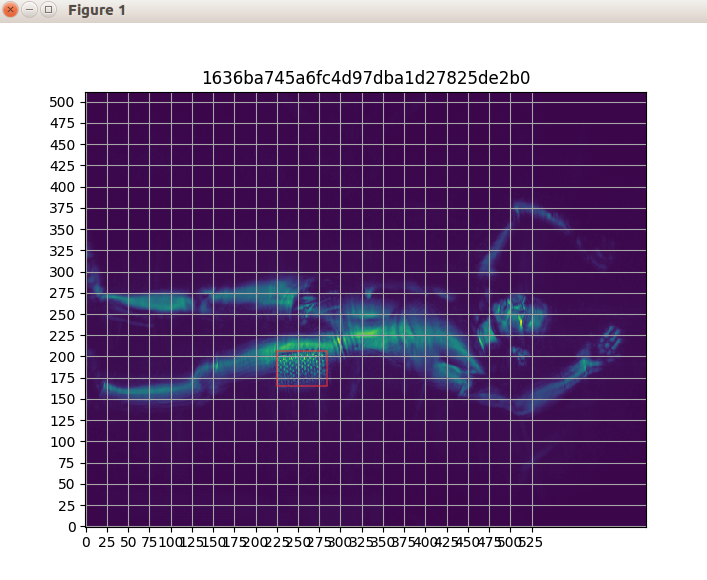
Figure 2: Algorithm show a body with a threat located at red

TABLE I: Label zones and threats

body_Id	z_start	z_stop	zone	x_start	x_stop	y_start	y_stop
00360	88	127	14	290	340	350	373
0043d	444	475	1	354	435	260	288
0043d	75	139	14	125	195	200	250
0043d	208	279	9	130	150	275	300
00504	158	214	8	320	375	189	236

III-B3 Filter image and produce a Binary image

This step filters every slice of the body to get the Region of Interest (ROI). The scanned image comes with a lot of noise. To filter that noise and obtain the ROI result, the image is submitted to a threshold filter, this threshold cleans the image to produce the segmentation. Using a Gaussian convolution, the segmented image will be normalized, this means, this image will be cleaned from the noise and will produce a better result to obtain the ROI. After that, the segmented image will be imposed to a dilatation process that join the segmented parts of the same object, cleaning the background. Images below on table 2 exposes the flow of raw image before and after the threshold filter:

TABLE II: Process of cleaning and producing a binary image

Raw Image	Clean process	Binary image
	$\mathbf{c}[u,v]=\begin{cases}0&\mathbf{I}[u,v]<T\\ 1&\mathbf{I}[u,v]\geq T\end{cases}\forall(u,v)\in\mathbf{I}$

III-B4 Do the segmentation and label the Regions

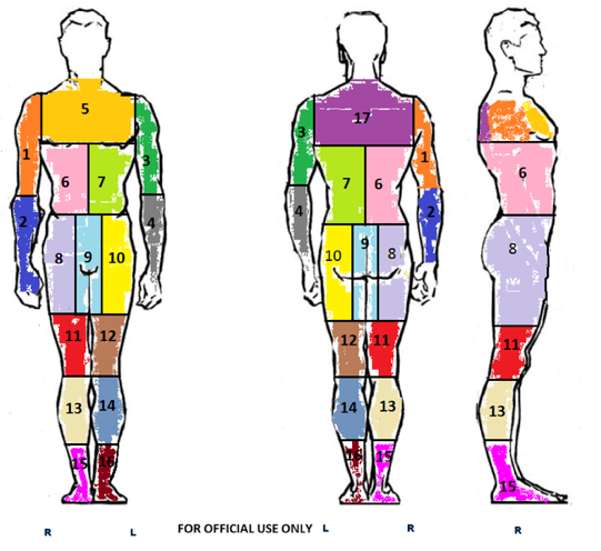
Figure 3: 17 zones of the bodies from kaggle TSA competition

On this step, the segmented image will be identified (labeled) in the right zone of the body, tracking the ROI through z axis. It starts taking a look at every ROI in the sliced image, separating them and combining in the right position on the z axis, it will produce a cloud of points of each zone of the human body. In that way, was produced 8 zones (through z axis) that represents the total human body. On the other hand, considering the x axis, was produced 16 zones, right and left side in a symmetric way and including a specific zone (zone 9 in figure 3) were completed the 17 zones.

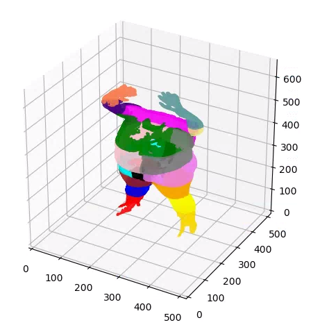
Figure 4: Final result of segmentation the body now has 17

To produce the right and left regions, was used a mask to guide the right ROI to the left ROI. Adding on this idea, the body was segmented on the z axis in a proportion of the total length of the body. In this way, the mask should guide in (x, y) position as well as the z axis position. The figure 3 shows the 17 zones of the human body. Each zone can have threat or not, so in this research, to classify the threat, were considered 34 zones, that is double the 17 zones of the body, it will be explain better on next steps.

The figure 4 shows the cloud of points of the 17 zones, that was segmented using the proportion of the height of each body.

III-B5 Multiply raw image with labeled image to save in the database

This step prepares the final image and save in a template directory to be loaded to a Digits interface. A Multiplication process get the labeled image and multiply with the raw image to get the real intensity of the image, it focuses on the ROI of the image. The table 3 shows the flow of the process:

TABLE III: Process of Multiply image

Raw Image	Binary image
Multiply process
$\boldsymbol{O}[u,v]=f\left(\boldsymbol{I}_{1}[u,v],\boldsymbol{I}_{2}[u,v]\right),\forall(u,v)\in\boldsymbol{I}_{1}$
Final image

After that, all sliced image are saved in directories zones and threat zones as showed at figure 5:

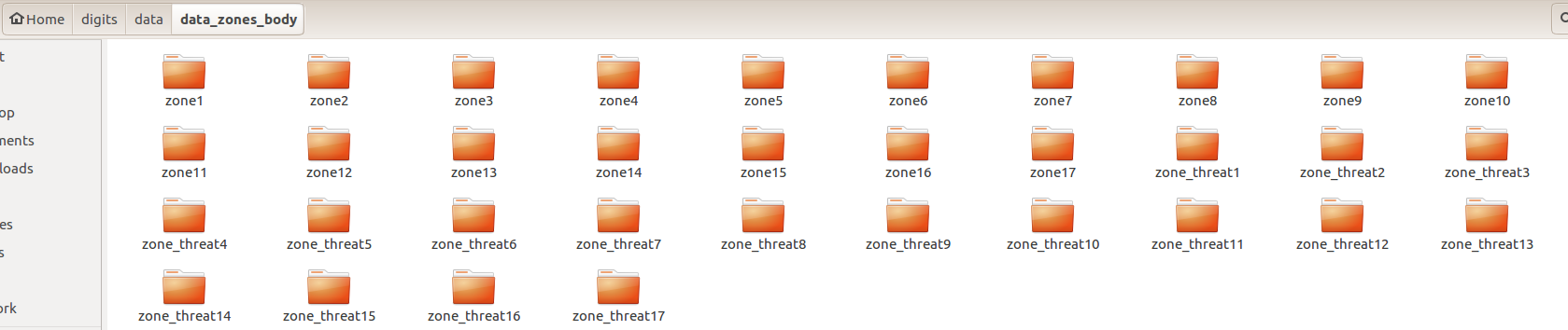
Figure 5: Directory division that contain zones

III-B6 Test and Training Dataset Classifier

After have all the zones labeled and written in a file, it can be loaded to fit a classification model. The training and test data will be separated in two portion: 60% and 40%. The training data will be with 60% of the total data and the test will take the rest of portion. The trained data was submitted in a configured model called CNN, with the solver type Stochastic Gradient Decent (SGD) using the network AlexNet and frame work Tensorflow. The AlexNet network consists of 7 layers, 5 convolutions by 5 max-pools and 2 regression layers at the end. The figure 6 shows the flow of AlexNet work:

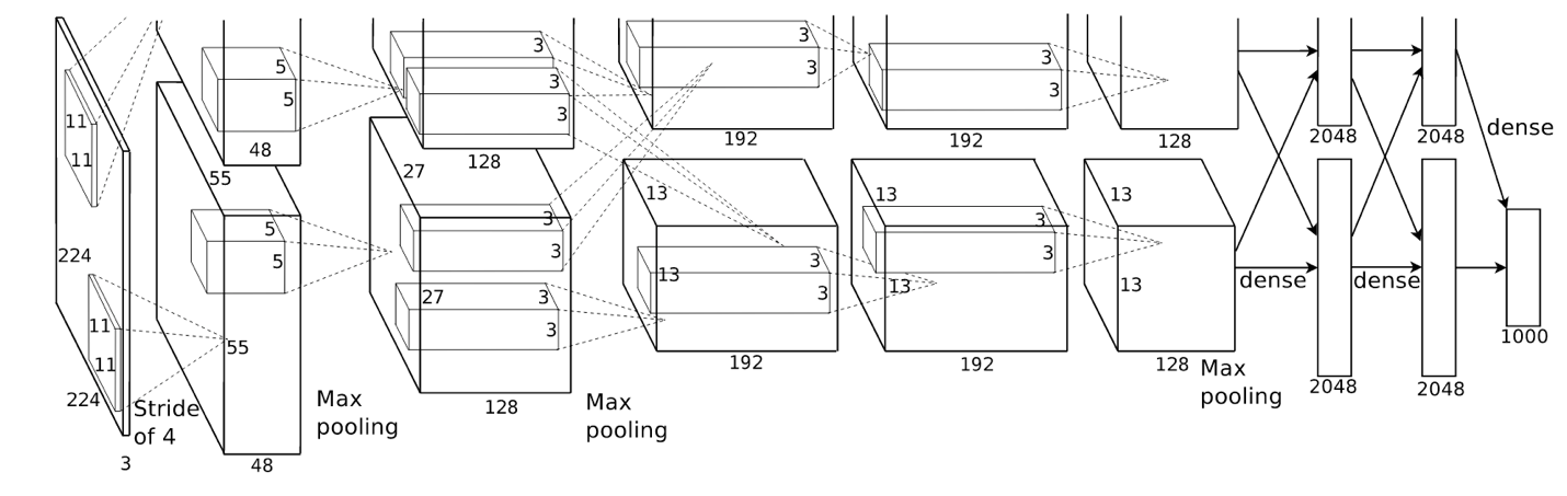
Figure 6: AlexNet [7] flow of convolution and pulling steps from the original paper.

AlexNet [7] has some advantages in the architecture that can be pointed:

1. It uses ReLU Non-linearity for non-saturating non-linearity, in this way, the training time of the gradient descent is much faster than the saturated non-linearitys.

2. It reduces the over-fitting using data augmentation and preserving transformation using label. Those transformation of the data do not need to be saved on a disk.

3. It dropout predictions, that is a very successful way to reduce test errors.

About the solver Stochastic Gradient Decent (SGD), Leon Bottou [10] point that the Big data size of learning is a bottleneck, so SGD can perform very well with train time.

Besides AlexNet, there are more libraries that also can be use to do machine learning:

• Digits from Nvidia, was used in this research, it is a IDE with a frame-network like caffe, torch, tensorflow and can choose models from their library. In this way, it can be chosen a particular model to training the dataset.

• Other libraries like scikit-learn that generate graphics like ROC, it can be access with this link http://scikit-learn.org/.

III-B7 Result Analysis

After the AlexNet process and CNN learning, a function model was produced here. This model could classify images in zones. Once the model was trained, we checked the accuracy on unseen test data. This was done using the confusion matrix evaluating the recall and precision of the trained model, comparing the predict class with the actual class. After obtained the metric it could use the ROC curve to compare the classifier. The results were saved and the curves was plotted using sckit learn python library.

IV Results

The database created here used a LMDB format and was loaded to produce a total of 287660 images that was submitted to training, validation and test. Below at figure 7, its shows the result of the split images (from Digits). Analyzing the 3 histograms, we can see that the data is unbalanced, especially with the threats. The Digits used a total of 34 zones (with threat or not). The training zones were fitted with a total of 172596 images (60%), using splitted images to train; to validation were used splitted images in a total of 57532 (20%) and for test was used 57534 images (20 %) and a format of 256x256 PNG image.

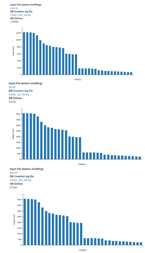
Figure 7: Histograms of images zones from DB train, Db Validation and DB Test.

The training, Validation and test were performed in a Ubuntu machine that has 16GB of memory, a I7 processor and a Nvidia GPU of 6GB. After 30 epochs, the model shows at the figure 8, an average accuracy for the validation data of 98.2863% and a loss of 0.091319. This was obtained with a shuffled data using AlexNet with Tensor-flow. The data transformation used a subtract mean image and data augmentation to do the flipping for the threat zones and produce more balance data, as well, using a contrast of 0.8 factor in the images.

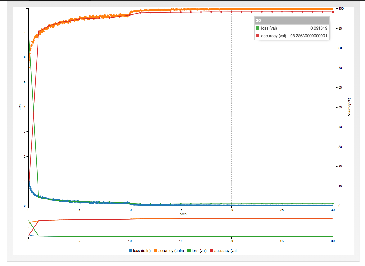
Figure 8: Graph of Loss and accuracy with 30 epochs.

After process the train with Digits, to test the model, we can use only 1 image. In figure 8, was used the Classify One Image to show Visualizations and Statistics when its selected. When running this process it will generate plots of weights from the responses of the network flow input image. Follow below the figure 9, it shows example output from the first layer.

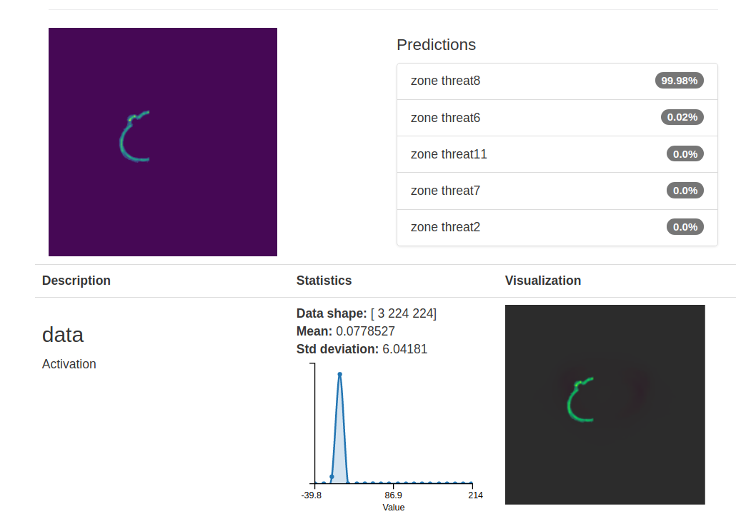
Figure 9: Classifying on image with statistics.

DIGITS plots statistical information in every convolution layer parameter, this include frequency, mean and standard deviation. This is a helpful tool to understand the results of convolution response applied in the input image. The classification results displayed at the figure 10 shows a response from the first convolution layer including the weights, activations and statistical information. “In a well-trained network, smooth filters without noisy patterns are usually discovered. A smooth pattern without noise is an indicator that the training process is sufficiently long, and likely no over-fitting occurred. In addition, visualization of the activation of the network’s features is a helpful technique to explore training progress. In deeper layers, the features become sparser and localized, and visualization helps to explore any potential dead filters (all zero features for many inputs).” (Sarraf and Tofigh [6]) The smoothness of the convolution images shows below follow the same pattern.

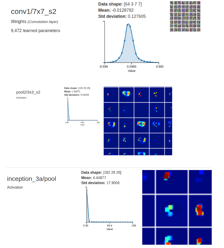
Figure 10: Statistics of the convolution, activations and weights.

To get a real result, it was used a different test data to enforce the validation of the model. The figure 11 shows the tops accuracy zones, it obtained a Top-1 accuracy of 99.31% and Top-5 accuracy of 100%.

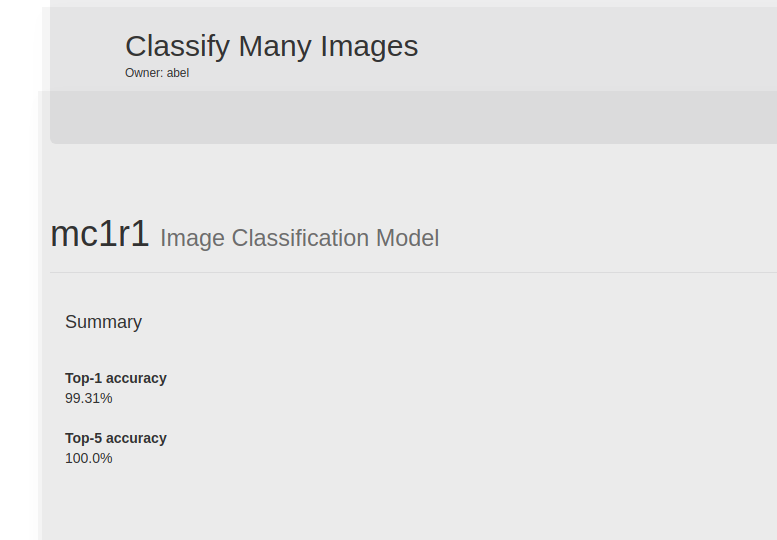
Figure 11: Classify many images summary.

After that, the confusion matrix at figure 12 shows all the accuracies by class zones, most of them has results upper to 98%.

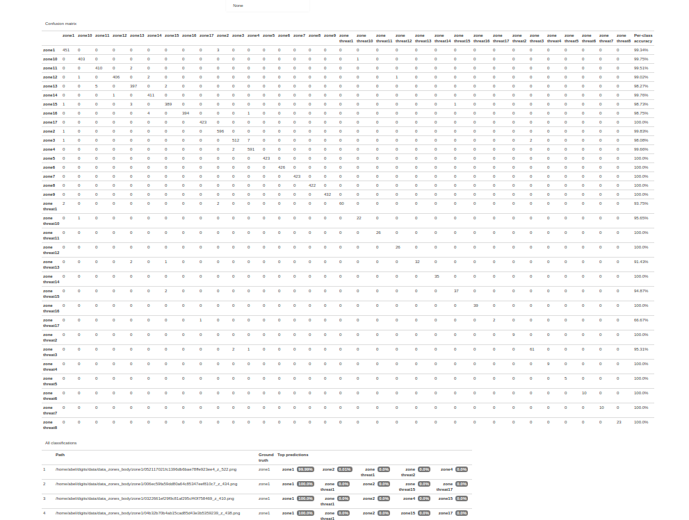
Figure 12: Confusion Matrix using classify many images summary from Digits.

Analyzing the 2 figures bellow: figure 13 and figure 14, we can obtain Recall and Precision of the model. Recall represents the true positives recovered from the true positives of the total sample, and Precision represents the true positives of the answer produced from the model. Starting with the analyses of Recall and Precision based on the results of Classifying Many Images Test and their Confusion Matrix, we can see the 2 graphs below. The figure 13 shows an average of 100% in Recall of the images as well as 100% in precision.

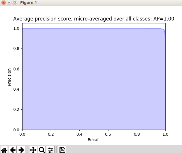
Figure 13: Average of Precision and Recall of bodies zone and zones with threats.

Figure 14 shows in more details all Precision and Recall by zones. It can be analyzed more precisely about how much true positives are recovering from the test images, as well as, the precision of this true positives. It can analyze all zones individually and most of them has a 100% in area for both rates.

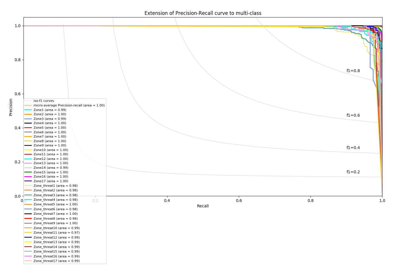
Figure 14: Precision and Recall of all zones and zones with threats.

V Conclusions

Considering the proposal in the Introduction of this research, this paper work intended to present a model to do the classification of the regions of the body’s images using supervised machine learning to identify the threats hired in the bodies. Moreover, produce an algorithm that fractionated the human body image in regions to be able to identify the body’s region correctly. In this paper work, it was developed a method to do the segmentation of the body in zones. It was presented 34 zones (considering 17 zones with left and right regions plus the threats zones) to do the learning process. Using robust module CNN with Stochastic Gradient Decent (SGD) and AlexNet, the model could learn the zones with threat or not. Combining with filters, the model could classify those zones of the bodies with a robust result that can help TSA agency security in all airports of North America and world. A big data files was used to train this deep learning to extract features using convolution neural network that can produce a faster learning provide by Nvidia Digits framework. One important point to be considered here is the fact that the model worked for the trained images of the sample used, it was not considered any external image.

Another point is that the result produced was highly accurate for predict zones, it can indicate an overfitting of learning. To prove that, it is necessary to do more test using external bodies, besides that the model need a balance data, that is, more information about the threats. This research showed in average an accuracy of 100% of the bodies zones, as well as, a recall and precision with the same 100% result for the most of zones. For future work, it is proposed here the follow: one classifier that combine two different models: one model that classify only the zones of the body and another model that only classifies the threat or not, increase the body images from external samples for produce a balance data.

VI Acknowledgements

This project is done as a part of Chang School Big Data Program.

I would like to express my gratitude towards Dr. Ghassem Tofigh, Ph.D. in Electrical and Computer Engineering, (Computer Vision and Pattern Recognition) from Ryerson University, and all fellows and professors from The G. Raymond Chang School of Continuing Education and Big Data Course. The algorithm for this research is available at https://github.com/abelguima/ryerson-capstone-CKME136

References

- [1] B. Elias, “Airport body scanners: The role of advanced imaging technology in airline passenger screening.” Congressional Research Service, Library of Congress, 2012.
- [2] P. Corke, Robotics, vision and control: fundamental algorithms in MATLAB. Springer, 2011, vol. 73.
- [3] D. M. Powers, “Evaluation: from precision, recall and f-measure to roc, informedness, markedness and correlation,” 2011.
- [4] J. Sauvola and M. Pietikäinen, “Adaptive document image binarization,” Pattern recognition, vol. 33, no. 2, pp. 225–236, 2000.
- [5] K. Robinson and P. F. Whelan, “Efficient morphological reconstruction: a downhill filter,” Pattern Recognition Letters, vol. 25, no. 15, pp. 1759–1767, 2004.
- [6] S. Sarraf and G. Tofighi, “Deep learning-based pipeline to recognize alzheimer’s disease using fmri data,” in Future Technologies Conference (FTC). IEEE, 2016, pp. 816–820.
- [7] A. Krizhevsky, I. Sutskever, and G. E. Hinton, “Imagenet classification with deep convolutional neural networks,” in Advances in neural information processing systems, 2012, pp. 1097–1105.
- [8] Y. LeCun, L. Bottou, Y. Bengio, and P. Haffner, “Gradient-based learning applied to document recognition,” Proceedings of the IEEE, vol. 86, no. 11, pp. 2278–2324, 1998.
- [9] Y. LeCun, L. Bottou, G. B. Orr, and K.-R. Müller, “Efficient backprop,” in Neural networks: Tricks of the trade. Springer, 1998, pp. 9–50.
- [10] L. Bottou, “Stochastic gradient descent tricks,” in Neural networks: Tricks of the trade. Springer, 2012, pp. 421–436.
- [11] Y. Bengio, “Practical recommendations for gradient-based training of deep architectures,” in Neural networks: Tricks of the trade. Springer, 2012, pp. 437–478.
- [12] K. Chellapilla, S. Puri, and P. Simard, “High performance convolutional neural networks for document processing,” in Tenth International Workshop on Frontiers in Handwriting Recognition. Suvisoft, 2006.
- [13] M. Abadi, A. Agarwal, P. Barham, E. Brevdo, Z. Chen, C. Citro, G. S. Corrado, A. Davis, J. Dean, M. Devin, S. Ghemawat, I. Goodfellow, A. Harp, G. Irving, M. Isard, Y. Jia, R. Jozefowicz, L. Kaiser, M. Kudlur, J. Levenberg, D. Mané, R. Monga, S. Moore, D. Murray, C. Olah, M. Schuster, J. Shlens, B. Steiner, I. Sutskever, K. Talwar, P. Tucker, V. Vanhoucke, V. Vasudevan, F. Viégas, O. Vinyals, P. Warden, M. Wattenberg, M. Wicke, Y. Yu, and X. Zheng, “TensorFlow: Large-scale machine learning on heterogeneous systems,” 2015, software available from tensorflow.org. [Online]. Available: https://www.tensorflow.org/
- [14] Y. Jia, E. Shelhamer, J. Donahue, S. Karayev, J. Long, R. Girshick, S. Guadarrama, and T. Darrell, “Caffe: Convolutional architecture for fast feature embedding,” in Proceedings of the 22nd ACM international conference on Multimedia. ACM, 2014, pp. 675–678.
- [15] C. M. Bishop, Pattern recognition and machine learning. springer, 2006.
- [16] J. Davis and M. Goadrich, “The relationship between precision-recall and roc curves,” in Proceedings of the 23rd international conference on Machine learning. ACM, 2006, pp. 233–240.
- [17] S. v. d. Walt, S. C. Colbert, and G. Varoquaux, “The numpy array: a structure for efficient numerical computation,” Computing in Science & Engineering, vol. 13, no. 2, pp. 22–30, 2011.