Optimal interpolation formulas in $W_{2}^{(m,m-1)}$ space

Abstract

In the present paper optimal interpolation formulas are constructed in $W_{2}^{(m,m-1)}(0,1)$ space. Explicit formulas for coefficients of optimal interpolation formulas are obtained. Some numerical results are presented.

MSC: 41A05, 41A15, 65D30, 65D32.

Keywords: optimal interpolation formula, optimal coefficients, the error functional, the extremal function.

1 Introduction: statement of the Problem

The typical problem of approximation is the interpolation problem. The classical method of its solution consists of construction of interpolation polynomials. However polynomials have some drawbacks as an instrument of approximation of functions with specifics and functions with small smoothness. It is proved that the sequence of the Lagrange polynomials, which constructed for concrete continues function for equally spaced nodes, by increasing of degree is not converge to the function. That is why splines are used instead of interpolation polynomials of high degree.

There are algebraic and variational approaches in the spline theory. In algebraic approach splines are considered as some smooth piecewise polynomial functions. In variational approach splines are elements of Hilbert or Banach spaces minimizing certain functionals. The first spline functions were constructed from pieces of cubic polynomials. After that, this construction was modified, the degree of polynomials increased, but the idea of their constructions remains permanently. The next essential step in the theory of splines was Hollyday’s result Hol57 , connecting Schoenberg’s cubic splines with the solution of the variational problem on minimum of square of a function norm from the space $L_{2}^{(2)}$. Further, the Hallyday result was generalized by Carl de Boor deBoor63 . Further, a large number of papers appeared, where, depending on specific requirements, the variational functional was modified. The theory of splines based on variational methods studied and developed, for example, by Ahlberg et al Ahlb67 , Arcangeli et al Arc04 , Attea Attea92 , A.V.Bezhaev and V.A.Vasilenko BezhVas01 , C. de Boor deBoor78 , M.I.Ignatev and A.B.Pevniy Ign91 , P.J.Laurent Lor75 , I.Schoenberg Schoen64 , L.L.Schumaker Schum07 , S.T.Stechkin and Yu.N.Subbotin Stech76 and others.

The present paper is devoted to a variational method. Here we construct optimal interpolation formulas.

Assume we are given the table of the values $\varphi(x_{\beta})$, $\beta=0,1,...,N$ of functions $\varphi$ at points $x_{\beta}\in[0,1]$. It is required approximate functions $\varphi$ by another more simple function $P_{\varphi}$, i.e.

$$\varphi(x)\cong P_{\varphi}(x)=\sum\limits_{\beta=0}^{N}{C_{\beta}(x)\cdot\varphi(x_{\beta})},$$ (1)

which satisfies the following equalities

$$\varphi(x_{\beta})=P_{\varphi}(x_{\beta}),\ \beta=0,1,...,N.$$ (2)

Here $C_{\beta}(x)$ and $x_{\beta}$ ($\in[0,1]$) are the coefficients and the nodes of the interpolation formula (1), respectively.

We suppose that functions $\varphi$ belong to the Hilbert space

$$W_{2}^{(m,m-1)}(0,1)=\{\varphi:[0,1]\to\mathbb{R}\ |\ \varphi^{(m-1)}\mbox{ is abs. cont. and }\varphi^{(m)}\in L_{2}(0,1)\},$$

equipped with the norm

$$\left\|{\varphi|W_{2}^{(m,m-1)}(0,1)}\right\|=\left\{{\int\limits_{0}^{1}{\left(\varphi^{(m)}(x)+\varphi^{(m-1)}(x)\right)}^{2}\,{\rm d}x}\right\}^{1/2}$$ (3)

and ${\int\limits_{0}^{1}{\left(\varphi^{(m)}(x)+\varphi^{(m-1)}(x)\right)}^{2}\,{\rm d}x}<\infty$. The equality (3) is the semi-norm and $\|\varphi\|=0$ if and only if $\varphi(x)=c_{0}+c_{1}x+...+c_{m-2}x^{m-2}+c_{m-1}e^{-x}$.

It should be noted that for a linear differential operator of order $m$, $L\equiv a_{m}\frac{\,{\rm d}^{m}}{\,{\rm d}x^{m}}+a_{m-1}\frac{\,{\rm d}^{m-1}}{\,{\rm d}x^{m-1}}+...+a_{1}\frac{\,{\rm d}}{\,{\rm d}x}+a_{0}$, $a_{m}\neq 0$, Ahlberg, Nilson and Walsh in the book (Ahlb67, , Chapter 6) investigated the Hilbert spaces in the context of generalized splines. Namely, with the inner product

$$\langle\varphi,\psi\rangle=\int_{0}^{1}L\varphi(x)\cdot L\psi(x)\,{\rm d}x.$$

The difference $\varphi-P_{\varphi}$ is called the error of the interpolation formula (1). The value of this error at a point $z\in[0,1]$ is the linear functional on the space $W_{2}^{(m,m-1)}(0,1)$, i.e.

$$(\ell,\varphi) = \varphi(z)-P_{\varphi}(z)=\varphi(z)-\sum\limits_{\beta=0}^{N}C_{\beta}(z)\varphi(x_{\beta})$$ (4)

$$= \int\limits_{-\infty}^{\infty}\left(\delta(x-z)-\sum\limits_{\beta=0}^{N}C_{\beta}(z)\delta(x-x_{\beta})\right)\varphi(x)\,{\rm d}x,$$

where $\delta(x)$ is the Dirac delta-function and

$$\ell(x,z)=\delta(x-z)-\sum\limits_{\beta=0}^{N}C_{\beta}(z)\delta(x-x_{\beta})$$ (5)

is the error functional of the interpolation formula (1) and belongs to the space ${W_{2}^{(m,m-1)*}}(0,1)$. The space ${W_{2}^{(m,m-1)*}}(0,1)$ is the conjugate to the space${W_{2}^{(m,m-1)}}(0,1)$. Further, for convenience, we denote $\ell(x,z)$ by $\ell(x)$.

By the Cauchy-Schwarz inequality the absolute value of the error (4) is estimated as follows

$$|(\ell,\varphi)|\leq\|\varphi|{W_{2}^{(m,m-1)}}\|\cdot\|\ell|{W_{2}^{(m,m-1)*}}\|,$$

where

$$\left\|{\ell|{W_{2}^{(m,m-1)*}}}\right\|=\mathop{\sup}\limits_{\varphi,\ \|\varphi\|\neq 0}\frac{|(\ell,\varphi)|}{\|\varphi\|}.$$

Therefore, in order to estimate the error of the interpolation formula (1) on functions of the space ${W_{2}^{(m,m-1)}}(0,1)$ it is required to find the norm of the error functional $\ell$ in the conjugate space ${W_{2}^{(m,m-1)*}}(0,1)$.

From here we get

Problem 1

Find the norm of the error functional $\ell$ of the interpolation formula (1) in the space ${W_{2}^{(m,m-1)*}}(0,1)$.

It is clear that the norm of the error functional $\ell$ depends on the coefficients $C_{\beta}(z)$ and the nodes $x_{\beta}$. The problem of minimization of the quantity $\|\ell\|$ by coefficients $C_{\beta}(z)$ is the linear problem and by nodes $x_{\beta}$ is, in general, nonlinear and complicated problem. We consider the problem of minimization of the quantity $\|\ell\|$ by coefficients $C_{\beta}(z)$ when nodes $x_{\beta}$ are fixed.

The coefficients $\mathring{C}_{\beta}(z)$ (if there exist) satisfying the following equality

$$\left\|\mathring{\ell}|{W_{2}^{(m,m-1)*}}\right\|=\mathop{\inf}\limits_{C_{\beta}(z)}\left\|\ell|{W_{2}^{(m,m-1)*}}\right\|$$ (6)

are called the optimal coefficients and corresponding interpolation formula

$$\mathring{P}_{\varphi}(z)=\sum\limits_{\beta=0}^{N}\mathring{C}_{\beta}(z)\varphi(x_{\beta})$$

is called the optimal interpolation formula in the space $W_{2}^{(m,m-1)*}(0,1)$.

Thus, in order to construct the optimal interpolation formula in the space ${W_{2}^{(m,m-1)}}(0,1)$ we need to solve the next problem.

Problem 2

Find the coefficients $\mathring{C}_{\beta}(z)$ which satisfy equality (6) when the nodes $x_{\beta}$ are fixed.

The main aim of the present paper is to construct the optimal interpolation formulas in ${W_{2}^{(m,m-1)}}(0,1)$ space and to find explicit formulas for optimal coefficients. First such a problem was stated and studied by S.L. Sobolev in Sob61a , where the extremal function of the interpolation formula was found in the Sobolev space $W_{2}^{(m)}$.

The rest of the paper is organized as follows. In Section 2 the extremal function which corresponds to the error functional $\ell$ is found and with its help representation of the norm of the error functional (5) is calculated, i.e. Problem 1 is solved; in Section 3 in order to find the minimum of $\left\|\ell\right\|^{2}$ by coefficients $C_{\beta}(z)$ the system of linear equations is obtained for the coefficients of optimal interpolation formulas (1) in the space $W_{2}^{(m,m-1)}(0,1)$, moreover existence and uniqueness of the solution of this system are proved; in Section 4 we give the algorithm for finding of coefficients of optimal interpolation formulas (1); Section 5 is devoted to calculation of optimal coefficients using the algorithm which is given in Section 4; finally, in Section 6 we give some numerical results which confirm the theoretical results of the present paper.

2 The extremal function and the norm of the error functional $\ell$

In this section we solve Problem 1, i.e. we find explicit form of the norm of the error functional $\ell$.

For finding the explicit form of the norm of the error functional $\ell$ in the space ${W_{2}^{(m,m-1)}}$ we use its extremal function which was introduced by Sobolev Sob61a ; Sob74 . The function $\psi_{\ell}$ from ${W_{2}^{(m,m-1)}}(0,1)$ space is called the extremal function for the error functional $\ell$ if the following equality is fulfilled

$$\left({\ell,\psi_{\ell}}\right)=\left\|{\ell\left|{{W_{2}^{(m,m-1)*}}}\right.}\right\|\cdot\left\|{\psi_{\ell}\left|{{W_{2}^{(m,m-1)}}}\right.}\right\|.$$

The space ${W_{2}^{(m,m-1)}}(0,1)$ is a Hilbert space and the inner product in this space is defined by the following formula

$$\langle{\varphi,\psi}\rangle=\int\limits_{0}^{1}\left(\varphi^{(m)}(x)+\varphi^{(m-1)}(x)\right)\left(\psi^{(m)}(x)+\psi^{(m-1)}(x)\right)\,{\rm d}x.$$ (7)

According to the Riesz theorem any linear continuous functional $\ell$ in a Hilbert space is represented in the form of a inner product. So, in our case, for any function $\varphi$ from ${W_{2}^{(m,m-1)}}(0,1)$ space, we have

$$\left({\ell,\varphi}\right)=\langle{\psi_{\ell},\varphi}\rangle$$ (8)

Here $\psi_{\ell}$ is the function from ${W_{2}^{(m,m-1)}}(0,1)$ is defined uniquely by functional $\ell$ and is the extremal function.

It is easy to see from (8) that the error functional $\ell$, defined on the space $W_{2}^{(m,m-1)}(0,1)$, satisfies the following equalities

$$(\ell,x^{\alpha})=0,\quad\alpha=0,1,...,m-2,$$ (9)

$$(\ell,\,{\rm e}^{-x})=0.$$ (10)

The equalities (9) and (10) mean that our interpolation formula is exact for the function $\,{\rm e}^{-x}$ and for any polynomial of degree $\leq m-2$.

The equation (8) was solved in Theorem 2.1 of ShadHay14 and for the extremal function $\psi_{\ell}$ was obtained the following expression

$$\psi_{\ell}(x)=(-1)^{m}\ell(x)*G_{m}(x)+P_{m-2}(x)+d\,{\rm e}^{-x},$$ (11)

where

$$G_{m}(x)=\frac{\mathrm{sgn}x}{2}\left(\frac{\,{\rm e}^{x}-\,{\rm e}^{-x}}{2}-\sum\limits_{k=1}^{m-1}\frac{x^{2k-1}}{(2k-1)!}\right),$$ (12)

$P_{m-2}(x)$ is a polynomial of degree $m-2$, $d$ is a constant and $*$ is the operation of convolution which for the functions $f$ and $g$ is defined as follows

$$f(x)*g(x)=\int\limits_{-\infty}^{\infty}f(x-y)g(y)\,{\rm d}y=\int\limits_{-\infty}^{\infty}f(y)g(x-y)\,{\rm d}y.$$

Now we obtain the norm of the error functional $\ell$. Since the space ${W_{2}^{(m,m-1)}}(0,1)$ is the Hilbert space then by the Riesz theorem we have

$$\left({\ell,\psi_{\ell}}\right)=\|\ell\|\cdot\|\psi_{\ell}\|=\|\ell\|^{2}.$$

Hence, using (5) and (11), taking into account (9) and (10), we get

$$\|\ell\|^{2} = (\ell,\psi_{\ell})=\int\limits_{-\infty}^{\infty}\ell(x,z)\psi_{\ell}(x)\,{\rm d}x$$

$$= \int\limits_{-\infty}^{\infty}\ell(x,z)\bigg{(}(-1)^{m}\bigg{[}G_{m}(x-z)-\sum\limits_{\beta=0}^{N}C_{\beta}(z)G_{m}(x-x_{\beta})\bigg{]}+P_{m-2}(x)+d\,{\rm e}^{-x}\bigg{)}\,{\rm d}x$$

$$= (-1)^{m}\int\limits_{-\infty}^{\infty}\left(\delta(x-z)-\sum\limits_{\beta=0}^{N}C_{\beta}(z)\delta(x-x_{\beta})\right)\left(G_{m}(x-z)-\sum\limits_{\beta=0}^{N}C_{\beta}(z)G_{m}(x-x_{\beta})\right)\,{\rm d}x.$$

Hence, keeping in mind that $G_{m}(x)$, defined by (12), is the even function, we have

$$\|\ell\|^{2}=(-1)^{m}\left(\sum\limits_{\beta=0}^{N}\sum\limits_{\gamma=0}^{N}C_{\beta}(z)C_{\gamma}(z)G_{m}(x_{\beta}-x_{\gamma})-2\sum\limits_{\beta=0}^{N}C_{\beta}(z)G_{m}(z-x_{\beta})\right).$$ (13)

Thus Problem 1 is solved.

Further, in next sections, we solve Problem 2.

3 Existence and uniqueness of optimal interpolation formula

Assume that the nodes $x_{\beta}$ of the interpolation formula (1) are fixed. The error functional (5) satisfies conditions (9) and (10). The norm of the error functional $\ell$ is multidimensional function with respect to the coefficients $C_{\beta}(z)$ $(\beta=\overline{0,N})$. For finding the point of the conditional minimum of the expression (13) under the conditions (9) and (10) we apply the Lagrange method.

Consider the function

$$\Psi(C_{0}(z),C_{1}(z),...,C_{N}(z),p_{0}(z),...,p_{m-2}(z),d(z))$$

$$\qquad=\left\|\ell\right\|^{2}-2(-1)^{m}\sum\limits_{\alpha=0}^{m-2}p_{\alpha}(z)\left({\ell,x^{\alpha}}\right)-2(-1)^{m}d(z)\left(\ell,\,{\rm e}^{-x}\right).$$

Equating to 0 the partial derivatives of the function $\Psi$ by $C_{\beta}(z)$ $(\beta=\overline{0,N})$, $p_{0},p_{1},...,p_{m-2}$ and $d$, we get the following system of linear equations

$$\sum\limits_{\gamma=0}^{N}C_{\gamma}(z)G_{m}(x_{\beta}-x_{\gamma})+\sum\limits_{\alpha=0}^{m-2}p_{\alpha}(z)x_{\beta}^{\alpha}+d(z)\,{\rm e}^{-x_{\beta}}=G_{m}(z-x_{\beta}),$$ (14)

$$\beta=0,1,...,N,$$

$$\sum\limits_{\gamma=0}^{N}C_{\gamma}(z)\ x_{\gamma}^{\alpha}=z^{\alpha},\ \alpha=0,1,...,m-2,$$ (15)

$$\sum\limits_{\gamma=0}^{N}C_{\gamma}(z)\ \,{\rm e}^{-x_{\gamma}}=\,{\rm e}^{-z},$$ (16)

where $G_{m}(x)$ is defined by equality (12).

The system (14)-(16) has a unique solution and this solution gives the minimum to $\left\|\ell\right\|^{2}$ under the conditions (15) and (16) when $N+1\geq m$.

The uniqueness of the solution of the system (14)–(16) is proved as the uniqueness of the solution of the system (26)–(28) of the work ShadHay14 .

Therefore, in fixed values of the nodes $x_{\beta}$ the square of the norm of the error functional $\ell$, being quadratic function of the coefficients $C_{\beta}(z)$, has a unique minimum in some concrete value $C_{\beta}(z)=\mathring{C}_{\beta}(z)$.

As it was said in the first section the interpolation formulas with the coefficients $\mathring{C}_{\beta}(z)$, corresponding to this minimum in fixed nodes $x_{\beta}$, is called the optimal interpolation formula and $\mathring{C}_{\beta}(z)$ are called the optimal coefficients.

Remark 1

It should be noted that by integrating both sides of the system (14)-(16) by $z$ from 0 to 1 we get the system (26)-(28) of the work ShadHay14 . This means that by integrating the optimal interpolation formula (1) in the space $W_{2}^{(m,m-1)}(0,1)$ we get the optimal quadrature formula of the form (1) in the same space (see ShadHay14 ).

Remark 2

It is clear from the system (14)-(16) that for the optimal coefficients the following are true

$$\mathring{C}_{\beta}(x_{\gamma}) = \delta_{\beta\gamma},\ \gamma=0,1,...,N,\ \ \beta=0,1,...,N,$$

$$p_{\alpha}(x_{\gamma}) = 0,\ \ \gamma=0,1,...,N,$$

where $\delta_{\beta\gamma}$ is the Kronecker symbol.

Below for convenience the optimal coefficients $\mathring{C}_{\beta}(z)$ we remain as $C_{\beta}(z)$.

4 The algorithm for computation of coefficients of optimal interpolation formulas

In the present section we give the algorithm for solution of the system (14)-(16). Here we use similar method suggested by S.L. Sobolev SobVas ; Sob77 for finding the coefficients of optimal quadrature formulas in the space $L_{2}^{(m)}(0,1)$. Below mainly is used the concept of discrete argument functions and operations on them. The theory of discrete argument functions is given in Sob74 ; SobVas . For completeness we give some definitions about functions of discrete argument.

Assume that the nodes $x_{\beta}$ are equal spaced, i.e. $x_{\beta}=h\beta,$ $h={1\over N}$, $N=1,2,...$.

Definition 1

The function $\varphi(h\beta)$ is a function of discrete argument if it is given on some set of integer values of $\beta$.

Definition 2

The inner product of two discrete argument functions $\varphi(h\beta)$ and $\psi(h\beta)$ is given by

$$\left[{\varphi(h\beta),\psi(h\beta)}\right]=\sum\limits_{\beta=-\infty}^{\infty}{\varphi(h\beta)\cdot\psi(h\beta)},$$

if the series on the right hand side converges absolutely.

Definition 3

The convolution of two functions $\varphi(h\beta)$ and $\psi(h\beta)$ is the inner product

$$\varphi(h\beta)*\psi(h\beta)=\left[{\varphi(h\gamma),\psi(h\beta-h\gamma)}\right]=\sum\limits_{\gamma=-\infty}^{\infty}{\varphi(h\gamma)\cdot\psi(h\beta-h\gamma)}.$$

Now we turn on to our problem.

Suppose that $C_{\beta}(z)=0$ when $\beta<0$ and $\beta>N$. Using above mentioned definitions we rewrite the system (14)-(16) in the convolution form

$$G_{m}(h\beta)*C_{\beta}(z)+\sum\limits_{\alpha=0}^{m-2}p_{\alpha}(z)(h\beta)^{\alpha}+d(z)\,{\rm e}^{-h\beta}=G_{m}(z-h\beta),$$ (17)

$$\beta=0,1,...,N,$$

$$C_{\beta}(z)=0,\quad\quad\beta<0,\ \ \beta>N$$ (18)

$$\sum\limits_{\beta=0}^{N}C_{\beta}(z)\cdot(h\beta)^{\alpha}=z^{\alpha},\ \ \ \alpha=0,1,...,m-2,$$ (19)

$$\sum\limits_{\beta=0}^{N}C_{\beta}(z)\cdot\,{\rm e}^{-h\beta}=\,{\rm e}^{-z}.$$ (20)

Thus we have the following problem.

Problem 3

Find the discrete functions $C_{\beta}(z)$, $\beta=0,1,...,N$, $p_{\alpha}(z)$, $\alpha=0,1,...,m-2$ and $d(z)$ which satisfy the system (17)-(20).

Further we investigate Problem 3 which is equivalent to Problem 2. Instead of $C_{\beta}(z)$ we introduce the following functions

$$v_{m}(h\beta) = G_{m}(h\beta)*C_{\beta}(z),$$ (21)

$$u_{m}(h\beta) = v_{m}\left({h\beta}\right)+\sum\limits_{\alpha=0}^{m-2}p_{\alpha}(z)(h\beta)^{\alpha}+d(z)\,{\rm e}^{-h\beta}.$$ (22)

Now we should express the coefficients $C_{\beta}(z)$ by the function $u(h\beta)$. For this we use the operator $D_{m}(h\beta)$ which satisfies the equality

$$D_{m}(h\beta)*G_{m}(h\beta)=\delta_{d}(h\beta),$$ (23)

where $\delta_{d}(h\beta)$ is equal to 0 when $\beta\neq 0$ and is equal to 1 when $\beta=0$, i.e. $\delta_{d}(h\beta)$ is the discrete delta-function.

In ShadHay04a ; ShadHay04b the operator $D_{m}(h\beta)$ which satisfies equation (23) is constructed and its some properties are studied.

The following theorems are proved in works ShadHay04a ; ShadHay04b .

Theorem 4.1

The discrete analogue of the differential operator ${{\,{\rm d}^{2m}}\over{\,{\rm d}x^{2m}}}-{{\,{\rm d}^{2m-2}}\over{\,{\rm d}x^{2m-2}}}$ satisfying the equation (23) has the form

$$D_{m}(h\beta)=\frac{1}{p_{2m-2}}\left\{\begin{array}[]{ll}\sum\limits_{k=1}^{m-1}A_{k}\lambda_{k}^{|\beta|-1},&|\beta|\geq 2,\\ -2\,{\rm e}^{h}+\sum\limits_{k=1}^{m-1}A_{k},&|\beta|=1,\\ 2C+\sum\limits_{k=1}^{m-1}\frac{A_{k}}{\lambda_{k}},&\beta=0,\end{array}\right.$$ (24)

where

$$C = 1+(2m-2)\,{\rm e}^{h}+\,{\rm e}^{2h}+\frac{\,{\rm e}^{h}\cdot p_{2m-3}}{p_{2m-2}},$$ (25)

$$A_{k} = \frac{2(1-\lambda_{k})^{2m-2}[\lambda_{k}(\,{\rm e}^{2h}+1)-\,{\rm e}^{h}(\lambda_{k}^{2}+1)]p_{2m-2}}{\lambda_{k}\ \mathcal{P}_{2m-2}^{\prime}(\lambda_{k})},$$ (26)

$$\mathcal{P}_{2m-2}(\lambda) = \sum\limits_{s=0}^{2m-2}p_{s}\lambda^{s}$$

$$= (1-\,{\rm e}^{2h})(1-\lambda)^{2m-2}-2(\lambda(\,{\rm e}^{2h}+1)-\,{\rm e}^{h}(\lambda^{2}+1))$$

$$\times\left[h(1-\lambda)^{2m-4}+\frac{h^{3}(1-\lambda)^{2m-6}}{3!}E_{2}(\lambda)+...+\frac{h^{2m-3}E_{2m-4}(\lambda)}{(2m-3)!}\right],$$

$p_{2m-2},\ p_{2m-3}$ are the coefficients of the polynomial $\mathcal{P}_{2m-2}(\lambda)$ defined by equality (4.1), $\lambda_{k}$ are the roots of the polynomial $\mathcal{P}_{2m-2}(\lambda)$ which absolute values less than 1, $E_{k}(\lambda)$ is the Euler-Frobenius polynomial of degree $k$ (the definition of the Euler-Frobenius polynomial is given, for example, in SobVas ).

Theorem 4.2

The discrete analogue $D_{m}(h\beta)$ of the differential operator ${{\,{\rm d}^{2m}}\over{\,{\rm d}x^{2m}}}-{{\,{\rm d}^{2m-2}}\over{\,{\rm d}x^{2m-2}}}$ satisfies the following equalities

1) $D_{m}(h\beta)*\,{\rm e}^{h\beta}=0,$

2) $D_{m}(h\beta)*\,{\rm e}^{-h\beta}=0,$

3) $D_{m}(h\beta)*(h\beta)^{n}=0,$ for $n=0,1,...,2m-3$,

4) $D_{m}(h\beta)*G_{m}(h\beta)=\delta_{d}(h\beta),$
here $G_{m}(h\beta)$ is the function of discrete argument corresponding to the function $G_{m}(x)$ defined by equality (12) and $\delta_{d}(h\beta)$ is the discrete delta-function.

Then taking into account (22), (23), using Theorems 4.1 and 4.2, for optimal coefficients we have

$$C_{\beta}(z)=D_{m}(h\beta)*u_{m}(h\beta).$$ (28)

Thus if we find the function $u_{m}(h\beta)$ then the optimal coefficients $C_{\beta}(z)$ will be found from equality (28).

In order to calculate the convolution (28) it is required to find the representation of the function $u_{m}(h\beta)$ for all integer values of $\beta$. From equality (17) we get that $u_{m}(h\beta)=G_{m}(z-h\beta)$ when $h\beta\in[0,1]$. Now we find the representation of the function $u_{m}(h\beta)$ when $\beta<0$ and $\beta>N$.

Since $C_{\beta}(z)=0$ when $h\beta\notin[0,1]$ then

$$C_{\beta}(z)=D_{m}(h\beta)*u_{m}(h\beta)=0,\,\,\,\,h\beta\notin[0,1].$$

Now we calculate the convolution $v_{m}(h\beta)=G_{m}(h\beta)*C_{\beta}(z)$ when $h\beta\notin[0,1]$.

Suppose $\beta\leq 0$ then taking into account equalities (12), (19) and (20), we have

$$v_{m}(h\beta) = \sum\limits_{\gamma=-\infty}^{\infty}{C_{\gamma}(z)\,G_{m}(h\beta-h\gamma)}$$

$$= -{1\over 2}\sum\limits_{\gamma=0}^{N}{C_{\gamma}(z)}\left({{{\,{\rm e}^{h\beta-h\gamma}-\,{\rm e}^{-h\beta+h\gamma}}\over 2}-\sum\limits_{k=1}^{m-1}{{{\left({h\beta-h\gamma}\right)^{2k-1}}\over{(2k-1)!}}}}\right)$$

$$= -{{\,{\rm e}^{h\beta}}\over 4}\ \,{\rm e}^{-z}+D\,{\rm e}^{-h\beta}+Q_{2m-3}(h\beta)+R_{m-2}(h\beta).$$

Thus when $\beta\leq 0$ we get

$$v_{m}(h\beta)=-{{\,{\rm e}^{h\beta}}\over 4}\ \,{\rm e}^{-z}+D\,{\rm e}^{-h\beta}+Q_{2m-3}(h\beta)+R_{m-2}(h\beta),$$ (29)

where

$$\begin{array}[]{rl}Q_{2m-3}(h\beta)=&\sum\limits_{i=0}^{2m-3}q_{i}(h\beta)^{i}\\[14.22636pt] =&{1\over 2}\left({\sum\limits_{k=1}^{\left[{{{m+1}\over 2}}\right]-1}{\sum\limits_{\alpha=0}^{2k-1}{{{(h\beta)^{2k-1-\alpha}(-1)^{\alpha}z^{\alpha}}\over{(2k-1-\alpha)!\cdot\alpha!}}}}}\right.+\left.{\sum\limits_{k=\left[{{{m+1}\over 2}}\right]}^{m-1}{\sum\limits_{\alpha=0}^{m-2}{{{(h\beta)^{2k-1-\alpha}(-1)^{\alpha}z^{\alpha}}\over{(2k-1-\alpha)!\cdot\alpha!}}}}}\right)\end{array}$$ (30)

is the polynomial of degree $2m-3$ with respect to $(h\beta)$,

$$\begin{array}[]{rl}R_{m-2}(h\beta)=&\sum\limits_{i=0}^{m-2}r_{i}(h\beta)^{i}\\ =&{1\over 2}\sum\limits_{k=\left[{{{m+1}\over 2}}\right]}^{m-1}{\sum\limits_{\alpha=m-1}^{2k-1}{{{(h\beta)^{2k-1-\alpha}(-1)^{\alpha}}\over{(2k-1-\alpha)!\cdot\alpha!}}}}\sum\limits_{\gamma=0}^{N}{C_{\gamma}(z)}(h\gamma)^{\alpha}\end{array}$$ (31)

is unknown polynomial of degree $m-2$ of $(h\beta)$,

$$D={1\over 4}\sum\limits_{\gamma=0}^{N}{C_{\gamma}(z)\,{\rm e}^{h\gamma}}.$$ (32)

Similarly, in the case $\beta\geq N$ for the convolution $v_{m}(h\beta)=G_{m}(h\beta)*C_{\beta}(z)$ we obtain

$$v_{m}(h\beta)={{\,{\rm e}^{h\beta}}\over 4}\ \,{\rm e}^{-z}-D\,{\rm e}^{-h\beta}-Q_{2m-3}(h\beta)-R_{m-2}(h\beta).$$ (33)

We denote

$$R_{m-2}^{-}(h\beta)=P_{m-2}(h\beta)+R_{m-2}(h\beta),\,\,\,\,\,\,a^{-}=d+D,$$ (34)

$$R_{m-2}^{+}(h\beta)=P_{m-2}(h\beta)-R_{m-2}(h\beta),\,\,\,\,\,\,a^{+}=d-D,$$ (35)

where $R_{m-2}^{-}(h\beta)=\sum\limits_{i=0}^{m-2}r_{i}^{-}(h\beta)^{i}$ and $R_{m-2}^{+}(h\beta)=\sum\limits_{i=0}^{m-2}r_{i}^{+}(h\beta)^{i}$.
Then taking into account (22), (29), (33) and the last notations (34), (35) we get the following problem.

Problem 4

Find the solution of the equation

$$D_{m}(h\beta)*u_{m}(h\beta)=0,\,\,h\beta\notin[0,1],$$ (36)

which has the form

$$u_{m}(h\beta)=\left\{\begin{array}[]{ll}-\frac{\,{\rm e}^{h\beta}}{4}\ \,{\rm e}^{-z}+a^{-}\,{\rm e}^{-h\beta}+Q_{2m-3}(h\beta)+R_{m-2}^{-}(h\beta),&\beta\leq 0,\\ G_{m}(z-h\beta),&0\leq\beta\leq N,\\ \frac{\,{\rm e}^{h\beta}}{4}\ \,{\rm e}^{-z}+a^{+}\,{\rm e}^{-h\beta}-Q_{2m-3}(h\beta)+R_{m-2}^{+}(h\beta),&\beta\geq N.\\ \end{array}\right.$$ (37)

Here $R_{m-2}^{-}(h\beta)$ and $R_{m-2}^{+}(h\beta)$ are unknown polynomials of degree $m-2$ with respect to $h\beta$, $a^{-}$ and $a^{+}$ are unknown constants.

If we find $R_{m-2}^{-}(h\beta)$, $R_{m-2}^{+}(h\beta)$, $a^{-}$ and $a^{+}$ then from (34), (35) we have

$$P_{m-2}(h\beta)=\frac{1}{2}\left(R_{m-2}^{-}(h\beta)+R_{m-2}^{+}(h\beta)\right),\ \ d=\frac{1}{2}(a^{-}+a^{+}),$$

$$R_{m-2}(h\beta)=\frac{1}{2}\left(R_{m-2}^{-}(h\beta)-R_{m-2}^{+}(h\beta)\right),\ \ D=\frac{1}{2}(a^{-}-a^{+}),$$

Unknowns $R_{m-2}^{-}(h\beta)$, $R_{m-2}^{+}(h\beta)$, $a^{-}$ and $a^{+}$ we will find from the equation (36), using the function $D_{m}(h\beta)$ defined by (24). Then we obtain explicit form of the function $u_{m}(h\beta)$ and find the optimal coefficients $C_{\beta}(z)$ ($\beta=0,1,...N$) from (28).

Thus Problem 4 and respectively Problems 3 and 2 will be solved.

In the next section we realize this algorithm for computation of coefficients $C_{\beta}(z)$ of optimal interpolation formulas (1).

5 Computation of coefficients of optimal interpolation formulas of the form (1)

In this section we give the solution of Problem 4 for any $m\in\mathbb{N}$ and $N\geq m-1$. We consider the cases $m=1$ and $m\geq 2$ separately.

First we consider the case $m=1$. For this case we have the following results

Theorem 5.1

Coefficients of the optimal interpolation formula (1) with equal spaced nodes in the space $W_{2}^{(1,0)}(0,1)$ have the following form

$$\begin{array}[]{ll}\mathring{C}_{\beta}(z)=&\frac{1}{2(1-\,{\rm e}^{2h})}\Bigg{[}\mathrm{sgn}(z-h\beta-h)\cdot(\,{\rm e}^{h\beta+2h-z}-\,{\rm e}^{z-h\beta})\\ &\qquad+\mathrm{sgn}(z-h\beta+h)\cdot(\,{\rm e}^{h\beta-z}-\,{\rm e}^{z-h\beta+2h})\\ &\qquad+(1+\,{\rm e}^{2h})\cdot\mathrm{sgn}(z-h\beta)\cdot(\,{\rm e}^{z-h\beta}-\,{\rm e}^{h\beta-z})\Bigg{]},\ \ \beta=0,1,...,N.\end{array}$$ (38)

Proof

Assume $m=1$. In this case the function $u_{m}(h\beta)$, given by equality (37), takes the form

$$u_{1}(h\beta)=\left\{\begin{array}[]{ll}-\frac{1}{4}\,{\rm e}^{h\beta-z}+a^{-}\,{\rm e}^{-h\beta},&\beta\leq 0,\\[5.69054pt] \frac{1}{4}\mathrm{sgn}(z-h\beta)\cdot(\,{\rm e}^{z-h\beta}-\,{\rm e}^{h\beta-z}),&0\leq\beta\leq N,\\[5.69054pt] \frac{1}{4}\,{\rm e}^{h\beta-z}+a^{+}\,{\rm e}^{-h\beta},&\beta\geq N\\ \end{array}\right.$$ (39)

and satisfies the equation

$$D_{1}(h\beta)*u_{1}(h\beta)=0\mbox{ for }\beta<0\mbox{ and }\beta>N,$$ (40)

where $D_{1}(h\beta)$ is defined by (24) when $m=1$:

$$D_{1}(h\beta)=\frac{2}{1-\,{\rm e}^{2h}}\left\{\begin{array}[]{ll}0,&|\beta|\geq 2,\\ -\,{\rm e}^{h},&|\beta|=1,\\ 1+\,{\rm e}^{2h},&\beta=0.\end{array}\right.$$ (41)

In (39) $a^{-}$ and $a^{+}$ are unknowns. From equation (40), using (39) and (41), for $\beta=-1$ and $\beta=N+1$ we respectively get

$$a^{-}=\,{\rm e}^{z}/4,\ \ a^{+}=-\,{\rm e}^{z}/4.$$ (42)

Then from (34), (35) taking into account (42) we obtain

$$d=0,\ \ D=\,{\rm e}^{z}/4.$$ (43)

Thus, putting (42) to (39) we have the following explicit form of the function $u_{1}(h\beta)$:

$$u_{1}(h\beta)=\left\{\begin{array}[]{ll}-\frac{1}{4}(\,{\rm e}^{h\beta-z}-\,{\rm e}^{z-h\beta}),&\beta\leq 0,\\[5.69054pt] \frac{1}{4}\mathrm{sgn}(z-h\beta)\cdot(\,{\rm e}^{z-h\beta}-\,{\rm e}^{h\beta-z}),&0\leq\beta\leq N,\\[5.69054pt] \frac{1}{4}(\,{\rm e}^{h\beta-z}-\,{\rm e}^{z-h\beta}),&\beta\geq N.\\ \end{array}\right.$$ (44)

Now from equality (28) we get

$$C_{\beta}(z)=D_{1}(h\beta)*u_{1}(h\beta),\ \ \beta=0,1,...,N.$$

Hence, using (41), (44) and computing the convolution $D_{1}(h\beta)*u_{1}(h\beta)$ for $\beta=0,1,...,N$ we get (38). Theorem 5.1 is proved.

Now we calculate the norm of the error functional $\ell$ on the space $W_{2}^{(1,0)}(0,1)$.

For $m=1$ taking into account (43) from (17) we have

$$\sum\limits_{\gamma=0}^{N}C_{\gamma}(z)G_{1}(h\beta-h\gamma)=G_{1}(z-h\beta),\ \ \beta=0,1,...,N.$$

Then from (13) using the last equality we get

$$\left\|\mathring{\ell}\right\|^{2} = -\left(\sum\limits_{\beta=0}^{N}C_{\beta}(z)\left[\sum\limits_{\gamma=0}^{N}C_{\gamma}(z)G_{1}(h\beta-h\gamma)-G_{1}(z-h\beta)\right]\right)+\sum\limits_{\beta=0}^{N}C_{\beta}(z)G_{1}(z-h\beta)$$

$$= \sum\limits_{\beta=0}^{N}C_{\beta}(z)G_{1}(z-h\beta).$$

Hence taking into account (12) we get the following

Theorem 5.2

The square of the norm of the error functional $\ell$ of the optimal interpolation formula (1) on the space $W_{2}^{(1,0)}(0,1)$ has the form

$$\left\|\mathring{\ell}|W_{2}^{(1,0)*}(0,1)\right\|^{2}=\frac{1}{4}\sum\limits_{\beta=0}^{N}\mathring{C}_{\beta}(z)\cdot\mathrm{sgn}(z-h\beta)\cdot(\,{\rm e}^{z-h\beta}-\,{\rm e}^{h\beta-z}),$$ (45)

where $\mathring{C}_{\beta}(z)$ are defined by (38).

Remark 3

We note that in Hay15 coincidence of the optimal interpolation formula of the form (1) in the space $W_{2}^{(1,0)}(0,1)$ with the interpolation spline $S_{1}(x)$, constructed in Theorem 3.2 of the work ShadHay13 , minimizing the semi-norm in this space is shown. The spline $S_{1}(x)$, constructed in Theorem 3.2 of ShadHay13 , is used in Avez10 to determine the total incident solar radiation at each time step and the temperature dependence of the thermophysical properties of the air and water.

Now we consider the case $m\geq 2$. In this case the following is true.

Theorem 5.3

Coefficients of optimal interpolation formulas (1) with equal spaced nodes $x_{\beta}=h\beta$ in the space $W_{2}^{(m,m-1)}(0,1)$ when $m\geq 2$ have the following form

$$\mathring{C}_{0}(z) = \frac{1}{p}\Bigg{[}2CG_{m}(z)-2\,{\rm e}^{h}\bigg{[}G_{m}(z-h)-\frac{1}{4}\,{\rm e}^{-h-z}+a^{-}\,{\rm e}^{h}+\sum\limits_{i=0}^{2m-3}q_{i}(-h)^{i}+\sum\limits_{i=0}^{m-2}r_{i}^{-}(-h)^{i}\bigg{]}$$

$$+\sum\limits_{k=1}^{m-1}\frac{A_{k}}{\lambda_{k}}\Bigg{\{}\sum\limits_{\gamma=0}^{N}\lambda_{k}^{\gamma}G_{m}(z-h\gamma)+M_{k}+\lambda_{k}^{N}N_{k}\Bigg{\}}\Bigg{]},$$

$$\mathring{C}_{\beta}(z) = \frac{1}{p}\Bigg{[}2CG_{m}(z-h\beta)-2\,{\rm e}^{h}\bigg{[}G_{m}(z-h(\beta-1))+G_{m}(z-h(\beta+1))\bigg{]}$$

$$+\sum\limits_{k=1}^{m-1}\frac{A_{k}}{\lambda_{k}}\Bigg{\{}\sum\limits_{\gamma=0}^{N}\lambda_{k}^{|\beta-\gamma|}G_{m}(z-h\gamma)+\lambda_{k}^{\beta}M_{k}+\lambda_{k}^{N-\beta}N_{k}\Bigg{\}}\Bigg{]},$$

$$\mathring{C}_{N}(z) = \frac{1}{p}\Bigg{[}2CG_{m}(z-1)-2\,{\rm e}^{h}\bigg{[}G_{m}(z-1+h)+\frac{1}{4}\,{\rm e}^{1+h-z}+a^{+}\,{\rm e}^{-1-h}$$

$$-\sum\limits_{i=0}^{2m-3}q_{i}(1+h)^{i}+\sum\limits_{i=0}^{m-2}r_{i}^{+}(1+h)^{i}\bigg{]}$$

$$+\sum\limits_{k=1}^{m-1}\frac{A_{k}}{\lambda_{k}}\Bigg{\{}\sum\limits_{\gamma=0}^{N}\lambda_{k}^{N-\gamma}G_{m}(z-h\gamma)+\lambda_{k}^{N}M_{k}+N_{k}\Bigg{\}}\Bigg{]},$$

where

$$M_{k} = \frac{\lambda_{k}\,{\rm e}^{-z}}{4(\lambda_{k}-\,{\rm e}^{h})}+\frac{a^{-}\lambda_{k}\,{\rm e}^{h}}{1-\lambda_{k}\,{\rm e}^{h}}+\sum\limits_{i=1}^{2m-3}q_{i}(-h)^{i}\sum\limits_{\nu=1}^{i}\frac{\lambda_{k}^{\nu}\Delta^{\nu}0^{i}}{(1-\lambda_{k})^{\nu+1}}+\frac{q_{0}\lambda_{k}}{1-\lambda_{k}}$$

$$\qquad\qquad\qquad+\sum\limits_{i=1}^{m-2}r_{i}^{-}(-h)^{i}\sum\limits_{\nu=1}^{i}\frac{\lambda_{k}^{\nu}\Delta^{\nu}0^{i}}{(1-\lambda_{k})^{\nu+1}}+\frac{r_{0}^{-}\lambda_{k}}{(1-\lambda_{k})},$$

$$N_{k} = \frac{\lambda_{k}\,{\rm e}^{1-z+h}}{4(1-\lambda_{k}\,{\rm e}^{h})}+\frac{a^{+}\lambda_{k}}{\,{\rm e}(\,{\rm e}^{h}-\lambda_{k})}-\sum\limits_{i=1}^{2m-3}q_{i}\sum\limits_{j=1}^{i}{i\choose j}h^{j}\sum\limits_{\nu=1}^{j}\frac{\lambda_{k}^{\nu}\Delta^{\nu}0^{j}}{(1-\lambda_{k})^{\nu+1}}-\sum\limits_{i=0}^{2m-3}q_{i}\frac{\lambda_{k}}{1-\lambda_{k}}$$

$$\qquad\qquad\qquad+\sum\limits_{i=1}^{m-2}r_{i}^{+}\sum\limits_{j=1}^{i}{i\choose j}h^{j}\sum\limits_{\nu=1}^{j}\frac{\lambda_{k}^{\nu}\Delta^{\nu}0^{j}}{(1-\lambda_{k})^{\nu+1}}+\sum\limits_{i=0}^{m-2}\frac{r_{i}^{+}\lambda_{k}}{(1-\lambda_{k})},$$

$$p = p_{2m-2}=1-\,{\rm e}^{2h}+2\,{\rm e}^{h}\left(h+\frac{h^{3}}{3!}+...+\frac{h^{2m-3}}{(2m-3)!}\right),$$

$$a^{-} = G_{m}(z)+\frac{1}{4}\,{\rm e}^{-z}-q_{0}-r_{0}^{-},$$

$$a^{+} = \,{\rm e}\left[G_{m}(z-1)-\frac{1}{4}\,{\rm e}^{1-z}+\sum\limits_{i=0}^{2m-3}q_{i}-\sum\limits_{i=0}^{m-2}r_{i}^{+}\right],$$

and $r_{i}^{-}$, $r_{i}^{+}$, $i=0,1,...,m-2$ satisfy the system (49) and (50) of $2m-2$ linear equations, $\lambda_{k},\ A_{k}$ and $C$ are given in Theorem 4.1, $q_{i}$ are defined by (30).

Proof

Here we find explicit form of $u_{m}(h\beta)$ then from (28), using $D_{m}(h\beta)$, we find optimal coefficients $C_{\beta}(z)$ .

In order to find $u_{m}(h\beta)$ we should find unknowns $r_{i}^{-},\ r_{i}^{+},$ $i=0,1,...,m-2$ and $a^{-}$, $a^{+}$. First we find $a^{-}$ and $a^{+}$. From (37) when $\beta=0$ and $\beta=N$ we get

$$a^{-} = G_{m}(z)+\frac{1}{4}\,{\rm e}^{-z}-q_{0}-r_{0}^{-},$$ (46)

$$a^{+} = \,{\rm e}\left(G_{m}(z-1)-\frac{1}{4}\,{\rm e}^{1-z}+\sum\limits_{i=0}^{2m-3}q_{i}-\sum\limits_{i=0}^{m-2}r_{i}^{+}\right).$$ (47)

Further, we find $2m-2$ unknowns $r_{i}^{-},\ r_{i}^{+},$ $i=0,1,...,m-2$. For $r_{i}^{-},\ r_{i}^{+},$ $i=0,1,...,m-2$ using (37), (46) and (47) from equation (36) we have the following system of $2m-2$ linear equations

$$\begin{array}[]{l}\sum\limits_{\gamma=1}^{\infty}D_{m}(h\beta+h\gamma)\bigg{[}\frac{\,{\rm e}^{-z}}{2}\sinh(h\gamma)+\,{\rm e}^{h\gamma}G_{m}(z)+\sum\limits_{i=0}^{2m-3}q_{i}(-h\gamma)^{i}-\,{\rm e}^{h\gamma}q_{0}\\ \qquad\qquad+\sum\limits_{i=0}^{m-2}r_{i}^{-}(-h\gamma)^{i}-\,{\rm e}^{h\gamma}r_{0}^{-}\bigg{]}+\sum\limits_{\gamma=0}^{N}D_{m}(h\beta-h\gamma)G_{m}(z-h\gamma)\\ \qquad\qquad+\sum\limits_{\gamma=1}^{\infty}D_{m}(h(N+\gamma-\beta))\bigg{[}\frac{\,{\rm e}^{1-z}}{2}\sinh(h\gamma)+\,{\rm e}^{-h\gamma}G_{m}(z-1)\\ \qquad\qquad+\sum\limits_{i=0}^{2m-3}q_{i}(\,{\rm e}^{-h\gamma}-(1+h\gamma)^{i})+\sum\limits_{i=0}^{m-2}r_{i}^{+}((1+h\gamma)^{i}-\,{\rm e}^{-h\gamma})\bigg{]}=0,\end{array}$$ (48)

where $\beta=-1,-2,...,-(m-1)$ and $\beta=N+1,N+2,...,N+m-1$.

From the system (48) in the cases $\beta=-1,-2,...,-(m-1)$ replacing $\beta$ by $-\beta$, using (24) and after some simplifications we have the following system of $m-1$ linear equations

$$\sum\limits_{i=0}^{m-2}B_{\beta i}^{-}r_{i}^{-}+\sum\limits_{i=0}^{m-2}B_{\beta i}^{+}r_{i}^{+}=T_{\beta},\ \beta=1,2,...,m-1,\\$$ (49)

where

$$\begin{array}[]{ll}B_{\beta 0}^{-}=&\sum\limits_{k=1}^{m-1}\frac{A_{k}}{\lambda_{k}}\sum\limits_{\gamma=1}^{\infty}\lambda_{k}^{|\beta-\gamma|}(1-\,{\rm e}^{h\gamma})+2C(1-\,{\rm e}^{h\beta})-2\,{\rm e}^{h}(2-\,{\rm e}^{h(\beta-1)}-\,{\rm e}^{h(\beta+1)}),\\ B_{\beta i}^{-}=&(-h)^{i}\left[2C\beta^{i}-2\,{\rm e}^{h}((\beta-1)^{i}+(\beta+1)^{i})+\sum\limits_{k=1}^{m-1}\frac{A_{k}}{\lambda_{k}}\sum\limits_{\gamma=1}^{\infty}\lambda_{k}^{|\beta-\gamma|}\gamma^{i}\right],\\ B_{\beta 0}^{+}=&\sum\limits_{k=1}^{m-1}\frac{A_{k}\lambda_{k}^{N+\beta}(\,{\rm e}^{h}-1)}{(1-\lambda_{k})(\,{\rm e}^{h}-\lambda_{k})},\\ B_{\beta i}^{+}=&\sum\limits_{k=1}^{m-1}\frac{A_{k}}{\lambda_{k}}\lambda_{k}^{N+\beta}\left(\sum\limits_{j=1}^{i}{i\choose j}h^{j}\sum\limits_{\nu=1}^{j}\frac{\lambda_{k}^{\nu}\Delta^{\nu}0^{j}}{(1-\lambda_{k})^{\nu+1}}+\frac{\lambda_{k}(\,{\rm e}^{h}-1)}{(1-\lambda_{k})(\,{\rm e}^{h}-\lambda_{k})}\right),\\ T_{\beta}=&-\Bigg{\{}\,{\rm e}^{-z}\bigg{[}C\sinh(h\beta)-\,{\rm e}^{h}\left[\sinh(h(\beta-1))+\sinh(h(\beta+1))\right]\bigg{]}+G_{m}(z)\left[2C\,{\rm e}^{h\beta}-2\,{\rm e}^{h}(\,{\rm e}^{h(\beta-1)}+\,{\rm e}^{h(\beta+1)})\right]\\ &+\sum\limits_{i=1}^{2m-3}q_{i}(-h)^{i}\bigg{[}2C\beta^{i}-2\,{\rm e}^{h}((\beta-1)^{i}+(\beta+1)^{i})\bigg{]}+q_{0}\bigg{[}2C(1-\,{\rm e}^{h\beta})-2\,{\rm e}^{h}(2-\,{\rm e}^{h(\beta-1)}-\,{\rm e}^{h(\beta+1)})\bigg{]}\Bigg{\}}\\ &-\sum\limits_{k=1}^{m-1}\frac{A_{k}}{\lambda_{k}}\Bigg{\{}\sum\limits_{\gamma=0}^{N}\lambda_{k}^{\gamma+\beta}G_{m}(z-h\gamma)+\sum\limits_{\gamma=1}^{\infty}\lambda_{k}^{|\beta-\gamma|}\bigg{[}\frac{\,{\rm e}^{-z}}{2}\sinh(h\gamma)+\,{\rm e}^{h\gamma}G_{m}(z)+\sum\limits_{i=1}^{2m-3}q_{i}(-h\gamma)^{i}+q_{0}(1-\,{\rm e}^{h\gamma})\bigg{]}\\ &+\lambda_{k}^{N+\beta}\bigg{[}\frac{\,{\rm e}^{1-z}\lambda_{k}\sinh(h)}{2(\lambda_{k}^{2}+1-2\lambda_{k}\cosh(h))}+\frac{\lambda_{k}}{\,{\rm e}^{h}-\lambda_{k}}G_{m}(z-1)+\sum\limits_{i=0}^{2m-3}q_{i}\left(\frac{\lambda_{k}(1-\,{\rm e}^{h})}{(\,{\rm e}^{h}-\lambda_{k})(1-\lambda_{k})}-\sum\limits_{j=1}^{i}{i\choose j}h^{j}\sum\limits_{\nu=1}^{j}\frac{\lambda_{k}^{\nu}\Delta^{\nu}0^{j}}{(1-\lambda_{k})^{\nu+1}}\right)\bigg{]}\Bigg{\}},\\ &\beta=1,2,...,m-1,\ \ i=1,2,...,m-2\end{array}$$

Now, from (48) in the cases $\beta=N+1,N+2,...,N+m-1$ replacing $\beta$ by $N+\beta$, using (24), doing some calculations we get the next system of $m-1$ linear equations

$$\sum\limits_{i=0}^{m-2}A_{\beta i}^{-}r_{i}^{-}+\sum\limits_{i=0}^{m-2}A_{\beta i}^{+}r_{i}^{+}=S_{\beta},\ \beta=1,2,...,m-1,$$ (50)

where

$$\begin{array}[]{ll}A_{\beta 0}^{-}=&\sum\limits_{k=1}^{m-1}\frac{A_{k}\lambda_{k}^{N+\beta}(1-\,{\rm e}^{h})}{(1-\lambda_{k})((1-\,{\rm e}^{h}\lambda_{k})},\\ A_{\beta i}^{-}=&(-h)^{i}\sum\limits_{k=1}^{m-1}\frac{A_{k}}{\lambda_{k}}\lambda_{k}^{N+\beta}\sum\limits_{\nu=1}^{i}\frac{\lambda_{k}^{\nu}\Delta^{\nu}0^{i}}{(1-\lambda_{k})^{\nu+1}},\\ A_{\beta 0}^{+}=&\sum\limits_{k=1}^{m-1}\frac{A_{k}}{\lambda_{k}}\sum\limits_{\gamma=1}^{\infty}\lambda_{k}^{|\beta-\gamma|}(1-\,{\rm e}^{-h\gamma})+2C(1-\,{\rm e}^{-h\beta})-2\,{\rm e}^{h}\bigg{[}2-\,{\rm e}^{-h(\beta-1)}-\,{\rm e}^{-h(\beta+1)}\bigg{]},\\ A_{\beta i}^{+}=&\sum\limits_{k=1}^{m-1}\frac{A_{k}}{\lambda_{k}}\sum\limits_{\gamma=1}^{\infty}\lambda_{k}^{|\beta-\gamma|}\bigg{[}\sum\limits_{j=1}^{i}{i\choose j}(h\gamma)^{j}+1-\,{\rm e}^{-h\gamma}\bigg{]}+2C\bigg{[}\sum\limits_{j=1}^{i}{i\choose j}(h\beta)^{j}+1-\,{\rm e}^{-h\beta}\bigg{]}\\ &-2\,{\rm e}^{h}\bigg{[}\sum\limits_{j=1}^{i}{i\choose j}\left((h(\beta-1))^{j}+(h(\beta+1))^{j}\right)+2-\,{\rm e}^{-h(\beta-1)}-\,{\rm e}^{-h(\beta+1))}\bigg{]},\\ S_{\beta}=&-\Bigg{\{}\,{\rm e}^{1-z}\bigg{[}C\sinh(h\beta)-\,{\rm e}^{h}\left[\sinh(h(\beta-1))+\sinh(h(\beta+1))\right]\bigg{]}+G_{m}(z-1)\left[2C\,{\rm e}^{-h\beta}-2\,{\rm e}^{h}(\,{\rm e}^{-h(\beta-1)}+\,{\rm e}^{-h(\beta+1)})\right]\\ &+\sum\limits_{i=0}^{2m-3}q_{i}\bigg{[}2C\bigg{(}\,{\rm e}^{-h\beta}-1-\sum\limits_{j=1}^{i}{i\choose j}(h\beta)^{j}\bigg{)}-2\,{\rm e}^{h}\bigg{(}\,{\rm e}^{-h(\beta-1)}+\,{\rm e}^{-h(\beta+1)}-2-\sum\limits_{j=1}^{i}{i\choose j}\left((h(\beta-1))^{j}+(h(\beta+1))^{j}\right)\bigg{)}\bigg{]}\Bigg{\}}\\ &-\sum\limits_{k=1}^{m-1}\frac{A_{k}}{\lambda_{k}}\Bigg{\{}\sum\limits_{\gamma=0}^{N}\lambda_{k}^{N+\beta-\gamma}G_{m}(z-h\gamma)+\lambda_{k}^{N+\beta}\bigg{[}\frac{\,{\rm e}^{-h}\lambda_{k}\sinh(h)}{2(\lambda_{k}^{2}+1-2\lambda_{k}\cosh(h))}+G_{m}(z)\frac{\lambda_{k}\,{\rm e}^{h}}{1-\,{\rm e}^{h}\lambda_{k}}+\sum\limits_{i=1}^{2m-3}q_{i}(-h)^{i}\sum\limits_{\nu=1}^{i}\frac{\lambda_{k}^{\nu}\Delta^{\nu}0^{i}}{(1-\lambda_{k})^{\nu+1}}\\ &+\frac{q_{0}\lambda_{k}(1-\,{\rm e}^{h})}{(1-\lambda_{k})(1-\lambda_{k}\,{\rm e}^{h})}\bigg{]}+\sum\limits_{\gamma=1}^{\infty}\lambda_{k}^{|\beta-\gamma|}\bigg{[}\frac{\,{\rm e}^{1-z}}{2}\sinh(h\gamma)+\,{\rm e}^{-h\gamma}G_{m}(z-1)+\sum\limits_{i=0}^{2m-3}q_{i}\left(\,{\rm e}^{-h\gamma}-1-\sum\limits_{j=1}^{i}{i\choose j}(h\gamma)^{j}\right)\bigg{]}.\\ &\beta=1,2,...,m-1,\ \ i=1,2,...,m-2,\end{array}$$

Further from (28), using (24) and (37) we get the optimal coefficients $C_{\beta}$, $\beta=0,1,...,N$, which are given in the assertion of the Theorem.

Theorem 5.3 is proved

For $m=2$ from Theorem 5.3 we get the following result which is Theorem 3 of Hay14 .

Corollary 1

(Theorem 3 of Hay14 ). Coefficients of optimal interpolation formula (1) with equal spaced nodes in the space $W_{2}^{(2,1)}(0,1)$ have the following form

$$\mathring{C}_{0}(z) = \frac{1}{p}\Bigg{\{}2CG_{2}(z)-2\,{\rm e}^{h}\bigg{[}G_{2}(z-h)-\frac{1}{4}\,{\rm e}^{-h-z}+a^{-}\,{\rm e}^{h}-\frac{1}{2}h+r_{0}^{-}\bigg{]}$$

$$+\frac{A_{1}}{\lambda_{1}}\bigg{[}\sum\limits_{\gamma=0}^{N}\lambda_{1}^{\gamma}G_{2}(z-h\gamma)+M_{1}+\lambda_{1}^{N}N_{1}\bigg{]}\Bigg{\}},$$

$$\mathring{C}_{\beta}(z) = \frac{1}{p}\Bigg{\{}2CG_{2}(z-h\beta)-2\,{\rm e}^{h}\bigg{[}G_{2}(z-h(\beta-1))+G_{2}(z-h(\beta+1))\bigg{]}$$

$$+\frac{A_{1}}{\lambda_{1}}\bigg{[}\sum\limits_{\gamma=0}^{N}\lambda_{1}^{|\beta-\gamma|}G_{2}(z-h\gamma)+\lambda_{1}^{\beta}M_{1}+\lambda_{1}^{N-\beta}N_{1}\bigg{]}\Bigg{\}},\ \ \beta=1,2,...,N-1,$$

$$\mathring{C}_{N}(z) = \frac{1}{p}\Bigg{\{}2CG_{2}(z-1)-2\,{\rm e}^{h}\bigg{[}G_{2}(z-1+h)+\frac{\,{\rm e}^{1+h}}{4\,{\rm e}^{z}}+\frac{a^{+}}{\,{\rm e}^{1+h}}-\frac{1}{2}(1+h)+r_{0}^{+}\bigg{]}$$

$$+\frac{A_{1}}{\lambda_{1}}\bigg{[}\sum\limits_{\gamma=0}^{N}\lambda_{1}^{N-\gamma}G_{2}(z-h\gamma)+\lambda_{1}^{N}M_{1}+N_{1}\bigg{]}\Bigg{\}},$$

where

$$M_{1} = \frac{\lambda_{1}\,{\rm e}^{-z}}{4(\lambda_{1}-\,{\rm e}^{h})}+\frac{a^{-}\lambda_{1}\,{\rm e}^{h}}{1-\lambda_{1}\,{\rm e}^{h}}-\frac{h\lambda_{1}}{2(1-\lambda_{1})^{2}}+\frac{r_{0}^{-}\lambda_{1}}{1-\lambda_{1}},$$

$$N_{1} = \frac{\lambda_{1}\,{\rm e}^{1-z+h}}{4(1-\lambda_{1}\,{\rm e}^{h})}+\frac{a^{+}\lambda_{1}}{\,{\rm e}(\,{\rm e}^{h}-\lambda_{1})}-\frac{h\lambda_{1}}{2(1-\lambda_{1})^{2}}-\frac{\lambda_{1}}{2(1-\lambda_{1})}+\frac{r_{0}^{+}\lambda_{1}}{1-\lambda_{1}},$$

$$\lambda_{1} = \frac{h(\,{\rm e}^{2h}+1)-\,{\rm e}^{2h}+1-(\,{\rm e}^{h}-1)\sqrt{h^{2}(\,{\rm e}^{h}+1)^{2}+2h(1-\,{\rm e}^{2h})}}{1-\,{\rm e}^{2h}+2h\,{\rm e}^{h}},$$

$$\begin{array}[]{ll}G_{2}(z)=\displaystyle\frac{\mathrm{sgn}z}{2}\bigg{(}\sinh z-z\bigg{)},&\displaystyle p=1-\,{\rm e}^{2h}+2h\,{\rm e}^{h},\\ C=\displaystyle 1+2\,{\rm e}^{h}+\,{\rm e}^{2h}-\frac{\,{\rm e}^{h}(\lambda_{1}^{2}+1)}{\lambda_{1}},&A_{1}=\displaystyle\frac{2(\lambda_{1}-1)(\lambda_{1}(\,{\rm e}^{2h}+1)-\,{\rm e}^{h}(\lambda_{1}^{2}+1))}{\lambda_{1}+1}\\ \displaystyle a^{-}=G_{2}(z)+\frac{\,{\rm e}^{-z}}{4}-r_{0}^{-},&\displaystyle a^{+}=\,{\rm e}\bigg{(}G_{2}(z-1)-\frac{\,{\rm e}^{1-z}}{4}-r_{0}^{+}+\frac{1}{2}\bigg{)},\\ \displaystyle r_{0}^{-}=\frac{T_{1}A_{10}^{+}-S_{1}B_{10}^{+}}{B_{10}^{-}A_{10}^{+}-B_{10}^{+}A_{10}^{-}},&\displaystyle r_{0}^{+}=\frac{S_{1}B_{10}^{-}-T_{1}A_{10}^{-}}{B_{10}^{-}A_{10}^{+}-B_{10}^{+}A_{10}^{-}},\\ \end{array}$$

here

$$B_{10}^{-} = 2C(1-\,{\rm e}^{h})-2\,{\rm e}^{h}(1-\,{\rm e}^{2h})+\sum\limits_{\gamma=1}^{\infty}A_{1}\lambda_{1}^{\gamma-2}(1-\,{\rm e}^{h\gamma}),$$

$$B_{10}^{+} = \frac{A_{1}\lambda_{1}^{N+1}(\,{\rm e}^{h}-1)}{(1-\lambda_{1})(\,{\rm e}^{h}-\lambda_{1})},$$

$$A_{10}^{-} = A_{1}\lambda_{1}^{N}\sum\limits_{\gamma=1}^{\infty}\lambda_{1}^{\gamma}(1-\,{\rm e}^{h\gamma}),$$

$$A_{10}^{+} = 2C(1-\,{\rm e}^{-h})-2\,{\rm e}^{h}(1-\,{\rm e}^{-2h})+\sum\limits_{\gamma=1}^{\infty}A_{1}\lambda_{1}^{\gamma-2}(1-\,{\rm e}^{-h\gamma}),$$

$$T_{1} = -\bigg{[}\,{\rm e}^{-z}(C\sinh(h)-\,{\rm e}^{h}\sinh(2h))+G_{2}(z)(2C\,{\rm e}^{h}-2\,{\rm e}^{h}(1+\,{\rm e}^{2h})-h(C-2\,{\rm e}^{h}))\bigg{]}$$

$$-\frac{A_{1}}{\lambda_{1}}\bigg{[}\sum\limits_{\gamma=0}^{N}\lambda_{1}^{\gamma+1}G_{2}(z-h\gamma)+\sum\limits_{\gamma=1}^{\infty}\lambda_{1}^{\gamma-1}\bigg{(}\frac{\,{\rm e}^{-z}\sinh(h\gamma)}{2}+\,{\rm e}^{h\gamma}G_{2}(z)-\frac{h\gamma}{2}\bigg{)}$$

$$+\lambda_{1}^{N+1}\bigg{(}\frac{\,{\rm e}^{1-z}\lambda_{1}\sinh(h)}{2(\lambda_{1}^{2}+1-2\lambda_{1}\cosh(h))}+\frac{\lambda_{1}G_{2}(z-1)}{\,{\rm e}^{h}-\lambda_{1}}+\frac{1}{2}\bigg{(}\frac{\lambda_{1}(1-\,{\rm e}^{h})}{(\,{\rm e}^{h}-\lambda_{1})(1-\lambda_{1})}-\frac{\lambda_{1}h}{(1-\lambda_{1})^{2}}\bigg{)}\bigg{)}\bigg{]},$$

$$S_{1} = -\bigg{[}\,{\rm e}^{1-z}(C\sinh(h)-\,{\rm e}^{h}\sinh(2h))+G_{2}(z-1)(2C\,{\rm e}^{-h}-2\,{\rm e}^{h}(1+\,{\rm e}^{-2h}))$$

$$+C(\,{\rm e}^{-h}-1-h)-\,{\rm e}^{h}(\,{\rm e}^{-2h}-1-2h)\bigg{]}-\frac{A_{1}}{\lambda_{1}}\bigg{[}\sum\limits_{\gamma=0}^{N}\lambda_{1}^{N-\gamma+1}G_{2}(z-h\gamma)$$

$$+\sum\limits_{\gamma=1}^{\infty}\lambda_{1}^{\gamma-1}\bigg{(}\frac{\,{\rm e}^{1-z}\sinh(h\gamma)}{2}+\,{\rm e}^{-h\gamma}G_{2}(z-1)+\frac{1}{2}(\,{\rm e}^{-h\gamma}-1-h\gamma)\bigg{)}$$

$$+\lambda_{1}^{N+1}\bigg{(}\frac{\,{\rm e}^{-z}\lambda_{1}\sinh(h)}{2(\lambda_{1}^{2}+1-2\lambda_{1}\cosh(h))}+\frac{\lambda_{1}\,{\rm e}^{h}G_{2}(z)}{1-\,{\rm e}^{h}\lambda_{1}}-\frac{\lambda_{1}h}{2(1-\lambda_{1})^{2}}\bigg{)}\bigg{)}\bigg{]}.$$

6 Numerical results

In this section we give some numerical results.

First, when $N=5$ using Theorem 5.1, Corollary 1 and Theorem 5.3 we get the graphs of the coefficients of the optimal interpolation formulas

$$\varphi(z)\cong\mathring{P}_{\varphi}(z)=\sum\limits_{\beta=0}^{5}\mathring{C}_{\beta}(z)\varphi(h\beta),\ z\in[0,1]$$

for the cases $m=1$, $m=2$ and $m=3$, respectively. They are presented in Figures 1, 4 and 7, respectively. These graphical results confirm Remark 2 for the cases $N=5$ and $m=1,2,3$, i.e. for the optimal coefficients the following hold

$$\mathring{C}_{\beta}(h\gamma)=\delta_{\beta\gamma},\ \ \beta,\gamma=0,1,...,5,$$

where $\delta_{\beta\gamma}$ is the Kronecker symbol.

Now, in numerical examples, we interpolate the functions

$$\varphi_{1}(z)=z^{2},\ \varphi_{2}(z)=\,{\rm e}^{2z}\mbox{ and }\varphi_{3}(z)=\sin z$$

by optimal interpolation formulas of the form (1) in the cases $m=1,\ 2,\ 3$ and $N=5,\ 10$, using Theorem 5.1, Corollary 1 and Theorem 5.3. For the functions $\varphi_{i}$, $i=1,2,3$ the graphs of absolute errors $|\varphi_{i}(z)-\mathring{P}_{\varphi_{i}}(z)|$, $i=1,2,3$, are given in Figures 2, 3, 5, 6, 8 and 9. In these Figures one can see that by increasing values of $m$ and $N$ absolute errors between optimal interpolation formulas and given functions are decreasing.

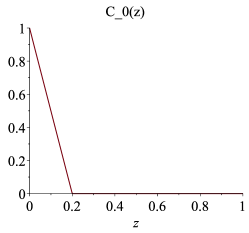
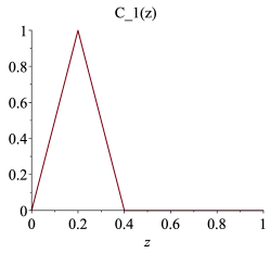
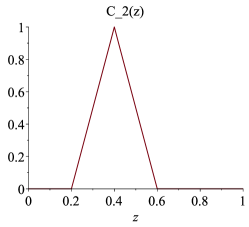
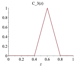
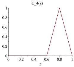
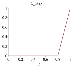
Figure 1: Graphs of coefficients of the optimal interpolation formulas (1) in the case $m=1$ and $N=5$.

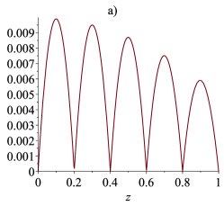
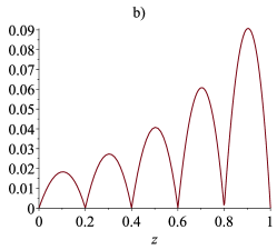
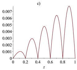
Figure 2: Graphs of absolute errors for $m=1$ and $N=5$: (a) $|\varphi_{1}(z)-P_{\varphi_{1}}(z)|$, (b) $|\varphi_{2}(z)-P_{\varphi_{2}}(z)|$, (c) $|\varphi_{3}(z)-P_{\varphi_{3}}(z)|$.

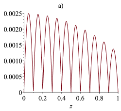
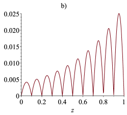
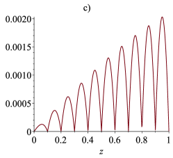
Figure 3: Graphs of absolute errors for $m=1$ and $N=10$: (a) $|\varphi_{1}(z)-P_{\varphi_{1}}(z)|$, (b) $|\varphi_{2}(z)-P_{\varphi_{2}}(z)|$, (c) $|\varphi_{3}(z)-P_{\varphi_{3}}(z)|$.

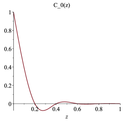
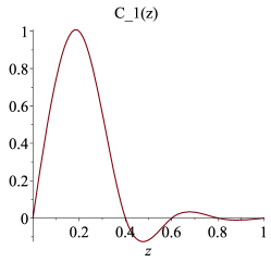
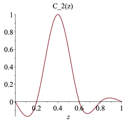
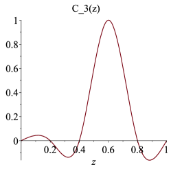
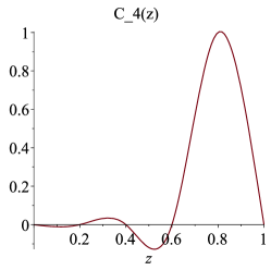
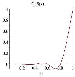
Figure 4: Graphs of coefficients of the optimal interpolation formulas (1) in the case $m=2$ and $N=5$.

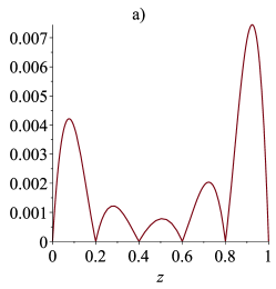
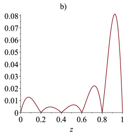
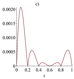
Figure 5: Graphs of absolute errors for $m=2$ and $N=5$: (a) $|\varphi_{1}(z)-P_{\varphi_{1}}(z)|$, (b) $|\varphi_{2}(z)-P_{\varphi_{2}}(z)|$, (c) $|\varphi_{3}(z)-P_{\varphi_{3}}(z)|$.

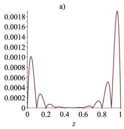
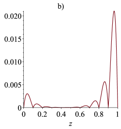
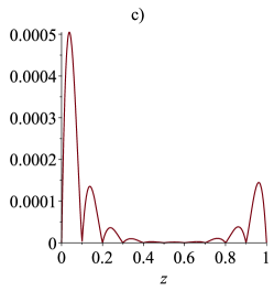
Figure 6: Graphs of absolute errors for $m=2$ and $N=10$: (a) $|\varphi_{1}(z)-P_{\varphi_{1}}(z)|$, (b) $|\varphi_{2}(z)-P_{\varphi_{2}}(z)|$, (c) $|\varphi_{3}(z)-P_{\varphi_{3}}(z)|$.

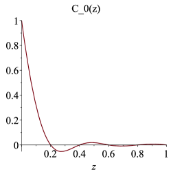
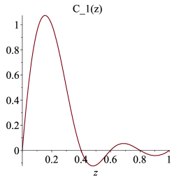
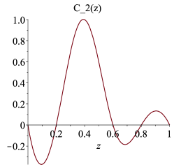
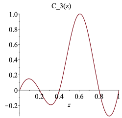
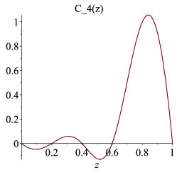
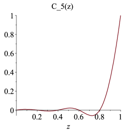
Figure 7: Graphs of coefficients of the optimal interpolation formulas (1) in the case $m=3$ and $N=5$.

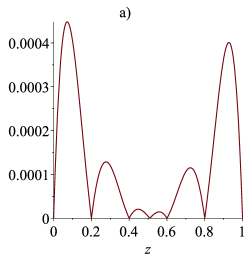
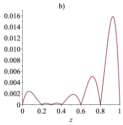
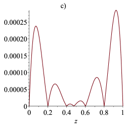
Figure 8: Graphs of absolute errors for $m=3$ and $N=5$: (a) $|\varphi_{1}(z)-P_{\varphi_{1}}(z)|$, (b) $|\varphi_{2}(z)-P_{\varphi_{2}}(z)|$, (c) $|\varphi_{3}(z)-P_{\varphi_{3}}(z)|$.

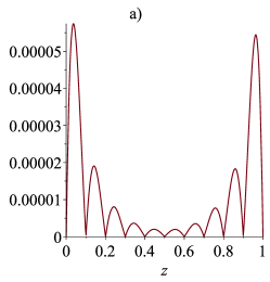
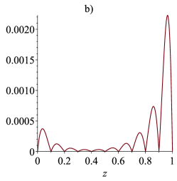
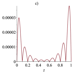
Figure 9: Graphs of absolute errors for $m=3$ and $N=10$: (a) $|\varphi_{1}(z)-P_{\varphi_{1}}(z)|$, (b) $|\varphi_{2}(z)-P_{\varphi_{2}}(z)|$, (c) $|\varphi_{3}(z)-P_{\varphi_{3}}(z)|$.

References

• (1) J.H.Ahlberg, E.N.Nilson, J.L.Walsh, The theory of splines and their applications, Mathematics in Science and Engineering, New York: Academic Press, 1967.
• (2) R.Arcangeli, M.C.Lopez de Silanes, J.J.Torrens, Multidimensional minimizing splines, Kluwer Academic publishers. Boston, 2004, 261 p.
• (3) M.Attea, Hilbertian kernels and spline functions, Studies in Computational Matematics 4, C. Brezinski and L.Wuytack eds, North-Holland, 1992.
• (4) N.R.Avezova, K.A.Samiev, A.R.Hayotov, I.M.Nazarov, Z.Zh.Ergashev, M.O.Samiev, Sh.I.Suleimanov, Modeling of the unsteady temperature conditions of solar greenhouses with a short-term water heat accumulator and its experimental testing, Applied Solar Energy, (2010) vol. 46, pp. 4 7.
• (5) A.Yu.Bezhaev, V.A.Vasilenko, Variational theory of splines, Springer Science - Business Media New York, (2001), 269 p.
• (6) C. de Boor, Best approximation properties of spline functions of odd degree, J. Math. Mech. 12, (1963), pp.747-749.
• (7) C. de Boor, A practical guide to splines, Springer-Verlag, 1978.
• (8) A.R.Hayotov, S.S.Babaev, Calculation of the coefficients of optimal interpolation formulas in the space $W_{2}^{(2,1)}(0,1)$, Uzbek Mathematical Journal, 2014, no.3, pp.126-133. (in Russian)
• (9) A.R.Hayotov, S.O.Kholova, N.H.Mamatova, An optimal interpolation formula and an interpolation spline minimizing the semi-norm in the space $W_{2}^{(1,0)}(0,1)$, Uzbek Mathematical Journal, 2015, no.2, pp.121-126. (in Russian)
• (10) J.C.Holladay, Smoothest curve approximation, Math. Tables Aids Comput. vol. 11. (1957) 223-243.
• (11) M.I.Ignatev, A.B.Pevniy, Natural splines of many variables, Nauka, Leningrad, 1991. (in Russian)
• (12) P.-J.Laurent, Approximation and Optimization, Mir, Moscow, 1975, 496 p. (in Russian)
• (13) I.J.Schoenberg, On trigonometric spline interpolation, J. Math. Mech. 13, (1964), pp.795-825.
• (14) L.L.Schumaker, Spline functions: basic theory, Cambridge university press, 2007, 600 p.
• (15) Kh.M.Shadimetov, A.R.Hayotov. Construction of the discrete analogue of the differential operator $d^{2m}/dx^{2m}-d^{2m-2}/dx^{2m-2}$. Uzbek Mathematical Journal, 2004, no.2, pp.85-95.
• (16) Kh.M.Shadimetov, A.R.Hayotov. Properties of the discrete analogue of the differential operator $d^{2m}/dx^{2m}-d^{2m-2}/dx^{2m-2}$. Uzbek Mathematical Journal. 2004, no.4, pp.72-83. (ArXiv.0810.5423v1 [math.NA])
• (17) Kh.M. Shadimetov, A.R. Hayotov, Construction of interpolation splines minimizing semi-norm in $W_{2}^{(m,m-1)}(0,1)$ space, BIT Nemrical Mathematics, 53 (2013), 545-563.
• (18) Kh.M. Shadimetov, A.R. Hayotov, Optimal quadrature fromulas in the sense of Sard in $W_{2}^{(m,m-1)}$ space, Calcolo, 51 (2014) 211-243.
• (19) S.L.Sobolev, On Interpolation of Functions of $n$ Variables, in: Selected Works of S.L.Sobolev, Springer, 2006, pp. 451-456.
• (20) S.L.Sobolev, Formulas of Mechanical Cubature in $n$- Dimensional Space, in: Selected Works of S.L.Sobolev, Springer, 2006, pp.445-450.
• (21) S.L.Sobolev, Introduction to the Theory of Cubature Formulas, Nauka, Moscow, 1974, 808 p.
• (22) S.L.Sobolev, V.L.Vaskevich. The Theory of Cubature Formulas. Kluwer Academic Publishers Group, Dordrecht (1997).
• (23) S.L.Sobolev, The coefficients of optimal quadrature formulas, in: Selected Works of S.L.Sobolev. Springer, 2006, pp.561-566.
• (24) S.B.Stechkin, Yu.N.Subbotin, Splines in computational mathematics, Nauka, Moscow, 1976, 248 p. (in Russian)
Refer to caption
Refer to caption
Refer to caption
Refer to caption
Refer to caption
Refer to caption