Dense Instanton-Dyon Liquid Model:
Diagrammatics

Abstract

We revisit the instanton-dyon liquid model in the confined phase by using a non-linear Debye-Huckel (DH) resummation for the Coulomb interactions induced by the moduli, followed by a cluster expansion. The organization is shown to rapidly converge and yields center symmetry at high density. The dependence of these results on a finite vacuum angle are also discussed. We also formulate the hypernetted chain (HCN) resummation for the dense instanton-dyon liquid and use it to estimate the liquid pair correlation functions in the DH limit. At very low temperature, the dense limit interpolates between chains and rings of instanton-anti-instanton-dyons and a bcc crystal, with strong topological and magnetic correlations.

I Introduction

This work is a continuation of our earlier studies LIU of the gauge topology in the confining phase of a theory with the simplest gauge group $SU(2)$. We suggested that the confining phase below the transition temperature is an “instanton dyon” (and anti-dyon) plasma which is dense enough to generate strong screening. The dense plasma is amenable to standard mean field methods.

The basic ingredients of the instanton-dyon liquid model are kVBLL instantons with finite holonomies KVLL . Diakonov and Petrov DP ; DPX have argued that the KvBLL instantons split into instanton-dyons in the confined phase below the critical temperature, and recombine above it in the deconfined phase. These observations have also been checked numerically LARSEN . The dissociation of instantons into constituents was advocated originally by Zhitnitsky and others ARIEL , and more recently by Unsal and collaborators UNSAL using controlled semi-classical approximations. When light quarks are added, center symmetry and chiral symmetry are found to be tied LIU ; SHURYAK1 ; SHURYAK2 ; TIN .

The purpose of this paper is to revisit the instanton-dyon liquid model without quarks, at low temperature in the center symmetric phase, through various many-body re-summations of the Coulomb interactions in the dense limit. In particular, we will show that the re-summations provide a specific interpolation between bion-like correlations in the dilute phase and mostly screened interactions in the dense phase.

In section II we briefly review the salient aspects of the instanton-dyon liquid model. We perform a non-linear Debye-Huckel re-summation of the coulomb interactions stemming from the moduli space, and combine them with a cluster expansion of the coulomb interactions originating from the streamlines. We show that the expansion is rapidly converging and the phase center symmetric already in the second cluster approximation. In section III we also show how multi-chain and rings can be further re-summed beyond the leading clusters and explicit them with some applications. In section IV, we extend our arguments to a finite vacuum angle $\theta$. In section V, we discuss a larger class of resummation pertinent for dense systems referred to as a hypernetted chain re-summation (HCN). In section VI, we suggest that a melted crystal of instanton-dyons and anti-instanton dyons may provide a semi-classical description of a Yang-Mills ensemble at very low temperature. Our conclusions are in section VII. In the Appendix we outline the elements for a future molecular dynamics simulation.

II Thermal Yang-Mills

The chief aspects of the instanton-dyon liquid model have been discussed in DP ; DPX ; LIU to which we refer for more details. Here, we briefly recall the key elements which will be useful in setting up the statistical Coulomb analysis using many-body techniques. For 2-colors the KvBLL instanton (anti-instanton) splits into $L,M$ ($\overline{L},\overline{M}$) instanton-dyons for large holonomies. $M$ carries $(+,+)$ and $L$ carries $(-,-)$ for (electric-magnetic) charges, with fractional topological charges $\nu$ and $\overline{\nu}=1-\nu$. The holonomy is fixed by the large x-asymptotics $\lim_{x\to\infty}\left<A_{4}^{3}\right>=2\pi T\nu\tau^{3}/2$ at fixed temperature $T$. In the confined phase with $\nu=\frac{1}{2}$ and moderate gauge coupling coupling $\alpha_{s}\leq 1$ the instanton-dyon actions $S_{L}=2\pi\nu/\alpha_{s}$ and $S_{M}=2\pi\overline{\nu}/\alpha_{s}$ are still large, justifying their use in a semi-classical description of the thermal Yang-Mills phase. Throughout the instanton- and antiinstanton-dyons will carry a finite core size which we will specify below.

A semi-classical ensemble of instanton-antiinstanton-dyons can be regarded as a statistical ensemble of semi-classical charges interacting mostly through their moduli space for like instanton- or aniti-instanton-dyons, and through streamlines for unlike instanton-anti-instanton-dyons. The grand partition function for such an ensemble is of the form (zero vacuum angle)

$${\cal Z}[T,f] \equiv\sum_{[K]}\prod_{i_{L}=1}^{K_{L}}\prod_{i_{M}=1}^{K_{M}}\prod_{i_{\bar{L}}=1}^{K_{\bar{L}}}\prod_{i_{\bar{M}}=1}^{K_{\bar{M}}}$$ (1)

$$\times\int\,\frac{fd^{3}x_{Li_{L}}}{K_{L}!}\frac{fd^{3}x_{Mi_{M}}}{K_{M}!}\frac{fd^{3}y_{{\bar{L}}i_{\bar{L}}}}{K_{\bar{L}}!}\frac{fd^{3}y_{{\bar{M}}i_{\bar{M}}}}{K_{\bar{M}}!}$$

$$\times e^{-V(x-y)+{\rm ln\,det}(G[x]G[y])}$$

The stream-line interactions $V$ are large and of order $1/\alpha_{s}$. They are attractive between like $D\overline{D}$ and repulsive between unlike $D\overline{D}$ LARS . Their relevant form for our considerations will be detailed below. In contrast, the moduli induced interactions captured in the $(K_{L}+K_{M})^{2}$ matrix $G[x]$, and in the $(K_{\bar{L}}+K_{\bar{M}})^{2}$ matrix $G[y]$ are of order $\alpha_{s}^{0}$. While the explicit form of these matrices can be found in DP ; DPX , it is sufficient to note here that these induced interactions are attractive between unlike instanton-dyons, and repulsive between like instanton-dyons. The bare fugacity $f$ will be regarded as an external parameter in what follows. Note that in the absence of $V$, ${\cal Z}\rightarrow{\cal Z}_{D}{\cal Z}_{\overline{D}}$ where each factor can be exactly re-written in terms of a 3-dimensional effective theory.

II.1 Effective action

The streamline interaction part $V$ can be bosonized using the complex fields $b\pm i\sigma$ through standard tricks. Here $b,\sigma$ refers to the Abelian magnetic and electric potentials stemming from the instanton-dyon charges. Also, each moduli determinant in (1) can be fermionized using ghost fields, and the ensuing Coulomb factors bosonized using complex $w,\overline{w}$ fields also through standard tricks as detailed in DP ; DPX . The net result of these repeated fermionization-bosonization procedures is an exact 3-dimensional effective action (p-space)

$$-S_{B}[b,\sigma,w,\bar{w}] =\int d^{3}p\bigg{[}\frac{1}{4}(b-i\sigma)V^{-1}(p)(b+i\sigma)$$

$$\qquad\qquad+\,4\pi\,\left(\nu fe^{w}+\overline{\nu}fe^{-w}\right)$$

$$\qquad\qquad+\,4\pi\,\left(\nu fe^{\bar{w}}+\overline{\nu}fe^{-\bar{w}}\right)\bigg{]}$$

subject to the constraint from the moduli (x-space)

$$-\frac{T}{4\pi}\nabla^{2}(w)+4\pi f\sinh(w)=\frac{T}{4\pi}\nabla^{2}(b-i\sigma)$$

$$-\frac{T}{4\pi}\nabla^{2}(\bar{w})+4\pi f\sinh(\bar{w})=\frac{T}{4\pi}\nabla^{2}(b+i\sigma)$$ (3)

(LABEL:1-3) allow to re-write exactly the partition function (1) in terms of a 3-dimensional effective theory. In LIU we have analyzed this partition function using the Debye-Huckel (one-loop) approximation. Here we will seek a more systematic organization of the dense phase described by (LABEL:1-3), that is more appropriate for the description of the confined phase at low temperature.

II.2 Cluster expansion

Our starting point is the linearization of (3) around $w=0$ which amounts to the solution

$$w(p)=\frac{p^{2}}{p^{2}+M^{2}}(b-i\sigma)(p)$$ (4)

with the squared screening mass $M^{2}=\frac{16\pi f}{T}$. Inserting (4) into (LABEL:1), we can carry the cluster expansion for the $4\pi f$ terms by integrating over the $b,\sigma$ fields as the measure is Gaussian in the partition function defined now in terms of the 3-dimensional effective action (LABEL:1). The result at second order is

$$\frac{\ln Z}{V_{3}} =8\pi f$$ (5)

$$+(4\pi f)^{2}(\nu^{2}+{\overline{\nu}}^{2})\int d^{3}r\,(e^{-V_{1}(r)}-1)$$

$$+(4\pi f)^{2}(2\nu\overline{\nu})\int d^{3}r\,(e^{-V_{2}(r)}-1)$$

with

$$V_{1}(p)=-V_{2}(p)=-\frac{p^{4}\,V(p)}{(p^{2}+M^{2})^{2}}$$ (6)

While the instanton-antiinstanton-dyon interaction is accessible numerically, for simplicity we will use here only its Coulomb asymptotic form $V(p)\approx\frac{4\pi C_{D}}{\alpha_{s}p^{2}}$ with $C_{D}=2$, so that

$$V_{1}(r)=-V_{2}(r)\approx\frac{MC_{D}}{2\alpha_{s}}\left(-\frac{2}{Mr}+1\right)e^{-Mr}$$ (7)

The large r-interaction between the pairs with magnetic charge 0 ($\bar{M}M$ and $\bar{L}L$) turns repulsive at large r, while that between the pairs with magnetic charge 2 ($\bar{M}L$ and $\bar{L}M$) turns attractive. Remarkably, the sign of the induced interaction between the pairs in (7) is flipped in comparison to the unscreened or bare interaction between the pairs, a sign of over-screening.

The chief effect of the moduli constraint (3-4) is to induce a non-linear Debye-Huckel screening effects between the charged instanton- and anti-instanton-dyons through the Mayer functions $e^{-V_{1,2}}-1$. This is a re-arrangement of the many-body dynamics that does not assume diluteness. In contrast, the cluster expansion in (5) is limited to the second cumulant and subsume diluteness in the ensemble of $D,\bar{D}$ but with non-linear Debye-Huckel effective interactions. This shortcoming will be addressed later.

For small $r$, we need to set a core for the attractive pair with magnetic charge 2. We choose the core to be $a=\frac{1}{T}$. As a result (5) plus the perturbative contribution reads

$$z_{b}(m,\nu)= \frac{\ln Z}{V_{3}T^{3}}-\frac{4\pi^{2}}{3}\nu^{2}{\overline{\nu}}^{2}$$

$$= \frac{m^{2}}{2}+F(m,\nu)-\frac{4\pi^{2}}{3}\nu^{2}{\overline{\nu}}^{2}$$ (8)

with $m=\frac{M}{T}$ and $V(x)=(-2/x+1)e^{-x}$ and

$$F(m,\nu) =\frac{\pi m}{4}(\nu^{2}+{\overline{\nu}}^{2})\int_{1}x^{2}(e^{-\frac{mC_{D}}{2\alpha_{s}}V(x)}-1)$$ (9)

$$+\frac{\pi m}{2}\nu\overline{\nu}\int_{c1}x^{2}(e^{\frac{mC_{D}}{2\alpha_{s}}V(x)}-1)$$

For $C_{D}\approx 2$ and $\alpha_{s}=1$, the transition from a center symmetric (confining) to a center asymmetric (deconfining) phase occurs for $m_{c}\approx$ 2.1, 2.3 for the two choices of the cutoff parameter $c1=1,0$. The choice $c1=0$ corresponds to the formal argument presented in UNSAL . In terms of the density of charged particles $n=8\pi f$, the transition occurs for $n\approx 2T^{3}$. For large density, the screening length scales like ${\sqrt{T}}/{\sqrt{n}}$, while the average separation scales like $1/{n^{\frac{1}{3}}}$. Our expansion is therefore justified. In Fig. 1 we show the behavior of the Polyakov line versus $m$ for the cutoff choice $c1=1$.

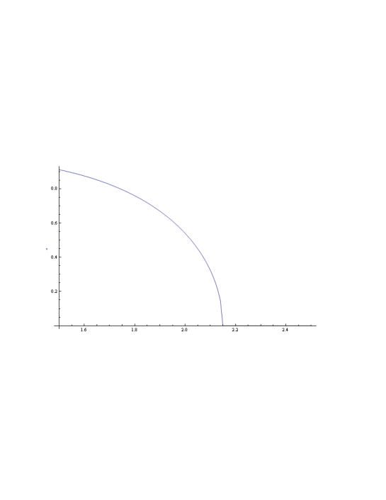
Figure 1: Polyakov line P=$|\cos(\pi\nu)|$ versus m.

III Open and closed chains

To go beyond the second cumulant approximation in (3) with bare fugacities, we will discuss in this section a systematic way for re-summing all tree diagrams between the charged particles, and also all ring diagrams with an arbitrary number of trees at the charged verticies. One of the chief effect of the resummation of all the trees is a re-definition of the fugacities of the charged particles as we will show below.

III.1 Diagrammatics

A systematic book-keeping procedure for the re-summation of all the trees and the rings with re-defined fugacities follows from a semi-classical treatment of the Coulomb-like field theory

$${\cal L}=-\frac{1}{2}{\bf\phi}^{T}{{\bf\cal V}}^{-1}{\bf\phi}+f_{1}(e^{i\phi_{1}}+e^{i\phi_{3}})+f_{2}(e^{i\phi_{2}}+e^{i\phi_{4}})$$ (10)

with $f_{1}=4\pi f\nu,f_{2}=4\pi f\bar{\nu}$, and the effective fields in 3-dimensions $\phi=(\phi_{1},\phi_{2},\phi_{3},\phi_{4})^{T}$,

$${\bf\cal V}=\left(\begin{array}[]{cc}0&{\bf V}\\ {\bf V}&0\end{array}\right)\qquad{\bf V}=\left(\begin{array}[]{cc}F_{1}&F_{2}\\ F_{2}&F_{1}\end{array}\right)$$ (15)

and the Mayer functions $-F_{1,2}=e^{-\beta V_{1,2}}-1$. The $4\times 4$ block-structure follows from the fact that the statistcal ensemble consists of 4-species of charged particles $D=L,M$ ($\bullet$) and $\bar{D}=\bar{L},\bar{M}$ $(\circ)$. The block off-diagonal character of ${\cal V}$ follows from the fact that the Mayer functions $-F_{1,2}$ resum the non-linear Debye-screening induced by the moduli between like-instanton-dyons, and are left acting only between unlike $D\bar{D}$ instanton-antiinstanton-dyons. It can be checked that (10) reproduces all Coulomb diagrams with the correct symmetry and weight factors as Feynman graphs when the vertices are linked by single lines only as illustrated in Figs. 2,3.

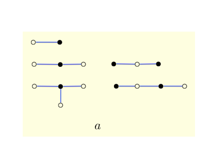
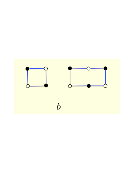
Figure 2: Typical open chain contributions to $\Omega_{\rm tree}$ (a), and closed chain or ring contributions to $\Omega_{ring}$ (b). $\bullet$ refers to $D=L,M$ and $\circ$ refers to $\bar{D}=\bar{L},\bar{M}$.

A re-summation of all trees and rings with arbitrary trees at the vertices amounts to a one-loop expansion around the saddle point approximation to (10) which is given by

$${\bf\phi}_{c}^{T}=i{\bf\cal V}(p=0)(f_{1}e^{i\phi_{1c}},f_{2}e^{i\phi_{2c}},f_{1}e^{i\phi_{3c}},e^{i\phi_{4c}})$$ (16)

Because of symmetry, the solution satisfies $\phi_{1}=\phi_{3}$, $\phi_{2}=\phi_{4}$. If we define $\alpha_{1}=i\phi_{1c},\alpha_{2}=i\phi_{2c}$ and use the symmetry, then (16) reads

$$\alpha_{1}=c_{1}f_{1}e^{\alpha_{1}}+c_{2}f_{2}e^{\alpha_{2}}$$

$$\alpha_{2}=c_{1}f_{2}e^{\alpha_{2}}+c_{2}f_{1}e^{\alpha_{1}}$$ (17)

Here

$$c_{1,2}=\int d^{3}x(e^{-\beta V_{1,2}}-1)$$ (18)

are the integrated Mayer functions. The saddle point contribution which resums all connected trees yield the pressure

$$\Omega_{\rm tree}=\frac{\ln Z_{\rm tree}}{V_{3}}=f_{1}e^{\alpha_{1}}(2-\alpha_{1})+f_{2}e^{\alpha_{2}}(2-\alpha_{2})$$ (19)

with $\alpha_{1,2}$ solutions to the non-linear classical equations (17). The resummed rings with arbitrary trees, follow by expanding (16) around the classical solution (17) to one-loop. The result is

$$\Omega_{\rm ring}=-\frac{1}{2}\int\frac{d^{3}p}{(2\pi)^{3}}(\ln(1+\mathbb{A})-\mathbb{A})$$ (20)

with in p-space

$$\mathbb{A}=-(\tilde{f}_{1}^{2}+\tilde{f}_{2}^{2})F_{1}^{2}+2\tilde{f}_{1}\tilde{f}_{2}F_{2}^{2}+\tilde{f}_{1}^{2}\tilde{f}_{2}^{2}(F_{1}^{2}-F_{2}^{2})^{2}$$ (21)

In the special case with $F\equiv F_{1}\approx-F_{2}$, the one-loop result simplifies

$$\mathbb{A}=-(\tilde{f}_{1}+\tilde{f}_{2})^{2}F^{2}$$ (22)

where $\tilde{f}_{1,2}=f_{1,2}e^{\alpha_{1,2}}$ are the tree-modified fugacites.

III.2 Approximations

The preceding expansion around the small fugacities follows by seeking the classical solution to (17) in powers $f_{1,2}$ or $\alpha_{1}\approx c_{1}f_{1}+c_{2}f_{2}$, $\alpha_{2}\approx c_{1}f_{2}+c_{2}f_{1}$. The tree contributions to the pressure in (19) to quadratic order are

$$\Omega_{\rm tree}\approx 2(f_{1}+f_{2})+c_{1}(f_{1}^{2}+f_{2}^{2})+2c_{2}f_{1}f_{2}$$ (23)

in agreement with (5). For large fugacities $f_{1,2}$ and for $c_{1}=-c_{2}=-c<0$, the solution to (20) satisfies $\alpha_{1}=-\alpha_{2}=\alpha$ with $\nu e^{\alpha}=\bar{\nu}e^{-\alpha}=\sqrt{\bar{\nu}\nu}$. As a result, the leading contribution in (5) is now changed to

$$8\pi f\rightarrow 8\pi\tilde{f}\equiv 8\pi f\sqrt{4\bar{\nu}\nu}$$ (24)

The resummation of all the trees for large bare fugacities amount to dressing the bare fugacities through $f\rightarrow\tilde{f}$ in a cluster expansion for the rings with no trees attached as illustrated in Fig. 2b. Some of the diagrams not included in the dressed fugacity expansion with ring-diagrams are illustrated in Fig. 3 which are of the 2-loop types. The first appear in the 5th cumulant, and the second in the 6th cumulant. So this re-organization resums a large class of diagrams, yet exact up to the 5th cumulant. Remarkably, in the center symmetric phase with $\nu=\bar{\nu}=\frac{1}{2}$, (24) amounts to the fugacity of non-interacting instanton- and anti-instanton-dyons, as all Coulomb interactions from the (linearized) moduli and the streamlines average out.

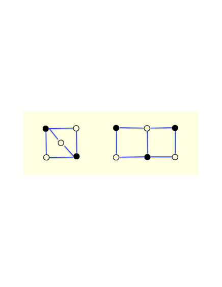
Figure 3: Examples of 2-loop contributions not included in the fugacity redefined 1-loop or ring re-summation.

In general, the solution to (17) for intermediate fugacities is not emanable analytically. One way to go beyond the second cumulant approximation (23) at low density is to insert the leading solutions $\alpha_{1}\approx c_{1}f_{1}+c_{2}f_{2}$, $\alpha_{2}\approx c_{1}f_{2}+c_{2}f_{1}$ in (19) without expanding the exponent,

$$\Omega_{\rm tree}\approx 4\pi f\left(\frac{1}{2}+b\right)(2Kb+2)e^{-2Kb}+(b\rightarrow-b)$$

(25)

where we have set $\nu=\frac{1}{2}+b$, $K=4\pi fc$, and noted that $c_{1}=-c_{2}=-c<0$. (25) resums all tree contributions with charge vertices that include an arbitrary number of 2-body links. (23) follows by expanding the exponents to first order in $f$. We note that (25) has always a maximum at $b=0$ or $\nu=\frac{1}{2}$ for positive $c$ which is center symmetric (confining). This conclusion remains unchanged when the ring contributions are added. Indeed, we note that the ring contribution (20) is an increasing function of the combination $\tilde{f}_{1}+\tilde{f}_{2}$ or more specifically

$$\tilde{f}_{1}+\tilde{f}_{2}\approx 8\pi f\left(\frac{1}{2}+b\right)e^{-2Kb}+8\pi f\left(\frac{1}{2}-b\right)e^{-2Kb}$$

(26)

with

$$2K=8\pi fc=\frac{2\pi}{m}\int dxx^{2}(e^{\frac{mC_{D}}{2\alpha_{s}}V(x)}-1)$$ (27)

using the previous notations. For $2K>4$ or $cf>\frac{1}{2\pi}$, this combination has a maximum away from 0 and competes against the classical contribution towards the center-symmetric solution. For $m<10$ we have $2K<4$. The ring contribution preserves center symmetry.

The center symmetric phase can be probed more acuratly by setting $\nu=\frac{1}{2}-b$. The semiclassical equation (26) reads

$$\alpha=-K\left(\frac{1}{2}+b\right)e^{\alpha}+K\left(\frac{1}{2}-b\right)e^{-\alpha}$$ (28)

At $b=0$ we have $\alpha=0$. We now can solve (28) by expanding exactly around $b=0$. Since $\alpha$ is an odd function of $b$, we seek a solution to (28) using $\alpha=x_{1}b+x_{2}b^{3}+...$, with $x_{1}$ satisfying

$$x_{1}= -2K-Kx_{1}$$ (29)

Since the leading contribution to the pressure is given by

$$\frac{\ln Z}{V_{3}}\approx 4\pi f\nu e^{\alpha}\left(1-\frac{\alpha}{2}\right)+4\pi f\bar{\nu}e^{-\alpha}\left(1+\frac{\alpha}{2}\right)+c.c$$

(30)

its expanded form to order ${\cal O}(b^{4})$ reads

$$\frac{\ln Z}{V_{3}}\approx 8\pi f-8\pi f\frac{2K}{K+1}b^{2}+{\cal O}(b^{4})$$

$$\rightarrow 8\pi f\left(\frac{1+K\sqrt{4\nu\bar{\nu}}}{1+K}\right)$$ (31)

where the last relation follows after restoring the full $\nu$ dependence. (31) shows that only the open chains with no tree-like-star insertions contribute to the leading $b^{2}$ and therefore $\sqrt{\nu\bar{\nu}}$ in the pressure. Note that (31) is independent of the integrated Mayer function $c$ in $K=4\pi fc$ in the center symmetric phase and/or large fugacities, in agreement with (24).

IV Finite vacuum angle $\theta$

At finite vacuum angle $\theta$, the bare fugacities for $\phi_{1,2}$ are now complex and given by $f_{1}=4\pi f\nu e^{\frac{i\theta}{2}}$ and $f_{2}=4\pi f\bar{\nu}e^{\frac{i\theta}{2}}$, while the bare fugacities for $\phi_{3,4}$ are their conjugate $f_{1,2}^{\dagger}$. For $c_{1}=c_{2}=-c<0$, we first note that the solution to the analogue of the classical equations (17) at finite $\theta$ satisfies $\alpha_{3,4}=\alpha_{1,2}^{\dagger}$, and $\alpha_{1}=-\alpha_{2}=\alpha$, with $\alpha$ complex and satisfying

$$\alpha=-Ke^{-i\frac{\theta}{2}}\overline{\nu}e^{\alpha^{\dagger}}+Ke^{-i\frac{\theta}{2}}\nu e^{-\alpha^{\dagger}}$$ (32)

The solution for small or large fugacities can be obtained analytically. We now discuss them sequentially.

IV.1 Large $K$

For large fugacities or large $K$, the solution to (32) in leading order gives $e^{\alpha}=\sqrt{\nu/\overline{\nu}}$ independently of $K$. In this limit, the summation of all the tree diagrams amount to a dressed fugacity with a leading (dimensionless) pressure

$$\frac{\ln Z}{V_{3}T^{3}}\rightarrow\frac{m^{2}}{2}\,\sqrt{4\nu\bar{\nu}}\,\cos\left({\theta}/{2}\right)-\frac{4\pi^{2}}{3}\nu^{2}{\overline{\nu}}^{2}$$ (33)

with $m^{2}=\frac{2n}{T^{3}}$ and including the perturbative contribution. (33) resums all the tree cumulant contributions at finite $\theta$ and is to be compared to (8-9) with only the second cumulant retained. (33) implies a transition from the center symmetric (confined) phase to the center asymmetric (deconfined) phase at a critical temperature

$$\frac{T_{c}(\theta)}{T_{c}(0)}=\left(\cos\left(\frac{\theta+2k\pi}{N_{c}}\right)\right)^{\frac{1}{3}}$$ (34)

with $T^{3}_{c}(0)=\frac{12n}{\pi^{2}}$ for $N_{c}=2$. Although our derivation was for $N_{c}=2$, our arguments for the re-summation of the trees extend to any $N_{c}$. Also, (33-34) were derived for $|\theta|<\pi$ in a $2\pi$-branch with $k=0$. The general result is multi-branch and $2\pi$-periodic following the substitution $\theta\rightarrow\theta+2k\pi$. Numerical lattice simulations have established that the transition temperature $T_{c}(\theta)$ decreases with $\theta$ as ($k=0$ branch)

$$\frac{T_{c}(\theta)}{T_{c}(0)}=1-R_{\theta}\theta^{2}+{\cal O}(\theta^{2})$$ (35)

with $R_{\theta}=0.0175(7)$ for $N_{c}=3$ NEGRO , in good agreement with $R_{\theta}=1/{6N_{c}^{2}}=0.0185$ from (34). Our result (34) is predictive of the $N_{c}$ dependence of $R_{\theta}$ and of the higher $\theta$ coefficients, with a cusp at $T_{c}(\pi)/T_{c}(0)=1/{2^{3}}$ at the CP symmetric point. This point is actually a tri-critical point where the CP breaking first order transition line at $\theta=\pi$ meets the first order transtion cusp from (34). Although (34) suggests that the CP transition line reduces to a point for $N_{c}=2$, this conclusion requires further amendments as it occurs at 0 temperature where the liquid is very dense requiring additional re-summations, some of which will be detailed below.

IV.2 Intermediate $K$

The onset of the center symmetric phase depends on the details of the arrangement of the parameters $K,\theta$, as (33) was only established for large $K$ or high density. The center symmetric phase can be probed more accuratly for different densities or $K$ by again setting $\nu=\frac{1}{2}-b$ in (32), and solving exactly around $b=0$. The result for the pressure to order ${\cal O}(b^{4})$ is

$$\frac{\ln Z}{V_{3}}=8\pi f\cos\frac{\theta}{2}-8\pi f\,2K\frac{K\cos\frac{\theta}{2}-1}{K^{2}-1}b^{2}+{\cal O}(b^{4})$$

(36)

which is seen to reduce to (31) at $\theta=0$. At finite vacuum angle $\theta$, the expanded result (36) develops a singularity at $K=4\pi fc=1$, the origin of which requires a more careful analysis.

In general, we have $\alpha_{1}=-\alpha_{2}$ and $\alpha_{3}=-\alpha_{4}$. At finite $\theta$, all $\alpha_{1,2,3,4}$ are complex and satisfy the coupled equations

$$\alpha_{1}= -Ke^{-i\frac{\theta}{2}}\nu e^{\alpha_{3}}+Ke^{-i\frac{\theta}{2}}\overline{\nu}e^{-\alpha_{3}}$$

$$\alpha_{3}= -Ke^{+i\frac{\theta}{2}}\nu e^{\alpha_{1}}+Ke^{+i\frac{\theta}{2}}\overline{\nu}e^{-\alpha_{1}}$$ (37)

At small $\theta$, these equations can be analyzed numerically by analytically continuing $\theta\rightarrow-i\theta$, so that

$$\alpha_{1}= -Ke^{-\frac{\theta}{2}}\left(\frac{1}{2}+b\right)e^{\alpha_{3}}+Ke^{-\frac{\theta}{2}}\left(\frac{1}{2}-b\right)e^{-\alpha_{3}}$$

$$\alpha_{3}= -Ke^{+\frac{\theta}{2}}\left(\frac{1}{2}+b\right)e^{\alpha_{1}}+Ke^{+\frac{\theta}{2}}\left(\frac{1}{2}-b\right)e^{-\alpha_{1}}$$

with $\alpha_{1,2,3,4}$ now all real. If we define

$$f(b,K,\theta,x)=-Ke^{-\frac{\theta}{2}}\left(\frac{1}{2}+b\right)e^{x}+Ke^{-\frac{\theta}{2}}\left(\frac{1}{2}-b\right)e^{-x}$$

(39)

Then $\alpha_{3}=x$ satisfies the transcendental equation

$$f(b,K,-\theta,f(b,K,\theta,x))-x=0$$ (40)

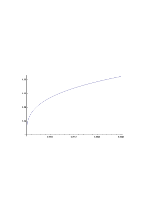
Figure 4: $x(b)$ as a function of $b$ for $K=1$, $\theta=0.1$ (upper) and $K=1.01$, $\theta=0.1$ (lower).

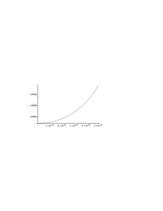
Figure 5: Pressure $\frac{\ln Z}{V_{3}}$ versus $b$ for $\theta=0.01$ and $K=0.99999$.

A numerical analysis of (40) reveals a solution with a 3-branch structure in the parameter space. In the region $b\ll 1$ around the center symmetric state, it turns out that for $K$ sufficiently close to 1 but less than 1 there exists a critical $b_{c}(K,\theta)$. For $b<b_{c}(K,\theta)$, the expansion leading to (36) is valid. However for $b>b_{c}(K,\theta)$, the branch which leads to (36) no longer exists, and the solution to (40) jumps to a third branch! For $K\geq 1$ and small $b$ only the third branch exists and will lead to the expansion (36) for $K>1$. For $K=1$, the solution is more tricky. In Fig. 4 we show the solution $x(b)$ at $\theta=0.1$ and $K=1$. In terms of the pressure, it is interesting to see if a ”window” appears for $K=1$. For imaginary $\theta$, we can see a ”window” for $(1/\cosh(\theta/2))<K<1$ numerically. Indeed, for $\theta=0.01$ and $K=0.99999$ we show in Fig. 5 the pressure $\frac{\ln Z}{V_{3}}$ versus $b$, with no maximum at $b=0$. In contrast, for $K$ outside the window, we always have $b=0$ as the maximum, which corresponds to the center symmetric phase. The window disappears for $\theta=0$. Its occurence at finite $\theta$ signals the incompleteness of the tree re-summation for $K$ in the range $(1/\cos(\theta/2))<K<1$ after analytical continuation.

V Hypernetted chains (HNC)

The static properties of a strongly coupled fluid are usually expressed in terms few-body reduced distribution functions of which the two-body distribution $g(\vec{r}_{1},\vec{r}_{2})$ or radial distribution $g(r_{12})$ is the standard example. The radial distribution function describes how the fluid density varies as a function of distance from a reference particle, providing a link between the microscopic content of the fluid and its macroscopic structure. $g(r_{12})$ can be obtained either from simulations using molecular dynamics (see below) or by solving the Ornstein-Zernicke (OZ) equation OZ subject to an additional closure relation. In this section we discuss such a closure in the form of the well-known hypernetted chain re-summation adapted to our dense dyon liquid. For that, we will provide a diagrammatic derivation based on our effective field theory (10).

V.1 Diagrammatic derivation

In the dense instanton-dyon liquid, the radial distribution following from the many-body analysis of (10) is a $4\times 4$ matrix with instanton-dyon entries $g^{ij}(r_{12})$. It is related to the irreducible density 2-point correlation function through

$$h^{ij}(r)=g^{ij}(r)-1\equiv e^{-\beta{\cal V}^{ij}(r)+\chi^{ij}(r)}-1$$ (41)

where the use of the barometric form in (41) defines $\chi^{ij}(r)$, and the $4\times 4$ matrix ${\cal V}$ is given in (15). $\chi^{ij}$ obeys a set of formal matrix equations

$$\chi^{ij}= \chi^{ij}_{a}+\chi^{ij}_{b}$$

$$\chi_{a}^{ij}= c^{il}\,\rho^{l}\,c^{lj}+c^{il}\,\rho^{l}\,c^{lm}\,\rho^{m}\,c^{mj}+....$$

$$c^{ij}= h^{ij}-\chi^{ij}_{a}$$ (42)

where $\rho^{ij}=\rho^{i}\delta^{ij}$ is a diagonal matrix with species density $\rho^{i}$. We now provide a diagrammatic derivation of (42) using the effective formulation (10).

The total pair correlation function $h^{ij}$ follows from summing all irreducible graphs with two external vertices fixed between $\vec{0}$ and $\vec{r}$. Between these two vertices we can hang an arbitrary number of independent 2-point functions as illustrated in Fig. 6a. The minimal insertion that cannot be decomposed into such a hanging structure is denoted by $-\beta{\cal V}+\chi$ with $\beta=\frac{1}{T}$. The diagrams contributing to $\chi$ can be separated in type-a and type-b. Type-a have at least one cutting point, i.e. a vertex that one can cut to split the diagram into two disconnected pieces as illustrated in Fig. 6b, while type-b have none as illustrated in Fig. 6c. For type-a, we can further count by enumerating the number of cutting points and define a summation over all possible 2-point diagrams that can be put between two nearest cutting points as $c(r)$, which defines the direct correlation function. It is readily seen that $c=h-\chi_{a}$. With these definitions in mind, simple diagrammatic arguments yield (42). The hypernetted chain approximation (HNC) amounts to setting $\chi_{b}=0$. In this case, (42) can be cast in the more standard form

$$h^{ij}= c^{ij}+c^{ik}\rho^{k}\star h^{kj}$$

$$c^{ij}= -\beta{\cal V}^{ij}+h^{ij}-\ln(1+h^{ij})$$ (43)

where $\star$ means convolution in x-space. The first of these equations is known as the Ornstein-Zernicke (OZ) equation, while the second equation as the HNC closure condition. The interaction energy per 3-volume and therefore the pressure can be re-constructed using the pair correlation function, for instance

$$\frac{\cal E}{V_{3}}=\left(\frac{2N}{V_{3}}\right)\,\frac{1}{2}\,\sum_{i,j}\int d^{3}r\,\beta{\cal V}^{ij}(r)h^{ij}(r)$$ (44)

V.2 Linear and non-linear DH approximations

The linear Debye-Huckel (DH) approximation follows by performing one iteration in the OZ equation with the initial condition $h=0$ or $c\approx-\beta{\cal V}$, to obtain formally in p-space

$$h_{DH}=\frac{-\beta{\cal V}}{1+\beta\rho{\cal V}}$$ (45)

For the instanton-dyon ensemble we have $\rho=\rho_{1}=\rho_{2}=M^{2}T/8$ and $V_{1}=-V_{2}=-V(p)=-\frac{8\pi p^{2}}{(p^{2}+M^{2})^{2}}$ in ${\cal V}$, so that

$$h_{DH} =\frac{\beta V}{1-(2\beta\rho V)^{2}}\left(\begin{array}[]{cc}{2\beta\rho V}&{1}\\ {1}&{2\beta\rho V}\end{array}\right)\otimes(1-\sigma_{1})$$ (48)

Here $\sigma_{1}$ is a Pauli matrix. (LABEL:DH1X) defines two independent pair correlation functions in p-space

$$h_{MM}=h_{LL}=-h_{ML}=\frac{2\rho\,(8\pi\beta)^{2}p^{4}}{(p^{2}+M^{2})^{4}-(16\pi\beta\rho)^{2}p^{4}}$$

$$h_{M\bar{M}}=h_{L\bar{L}}=-h_{M\bar{L}}=\frac{(8\pi\beta)\,p^{2}(p^{2}+M^{2})^{2}}{(p^{2}+M^{2})^{4}-(16\pi\beta\rho)^{2}p^{4}}$$

(50)

For $\rho={M^{2}T}/8$ the denominator

$$(p^{2}+M^{2})^{4}-4\pi^{2}p^{4}M^{4}$$ (51)

is negative for $p>\frac{M}{\sqrt{2\pi-1}}\approx\frac{M}{2}$. The spatial cutoff $a=\frac{1}{T}$ used earlier, translates to a p-cutoff of $T$. Since $M\approx 2T$, the negative range is physically not relevant. These observations are similar to the ones encountered in the DH analysis of the electric and magnetic correlation functions in LIU (first reference).

The HNC equations (43) allow to go beyond the DH approximation in the dense ensemble, but requires a numerical calculation. Here, we only mention that a simple non-linear correction to the DH result follows from (43) by retaining the leading correction to the direct correlation function, namely $c^{ij}\approx-\beta{\cal V}^{ij}+\frac{1}{2}(h^{ij})^{2}$, and use it to iterate the OZ equation after the substitution $h\rightarrow h_{DH}$. The net effect is a non-linear correction to the DH result (45) in p-space

$$h_{DH2}=\frac{-\beta{\cal V}+\frac{1}{2}h_{DH}^{2}}{1+\rho(\beta{\cal V}-\frac{1}{2}h_{DH}^{2})}$$ (52)

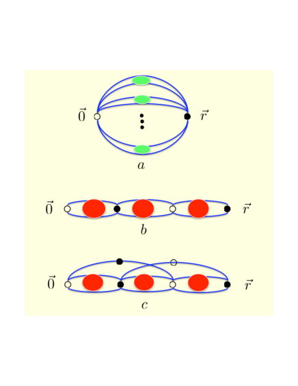
Figure 6: (a) Typical diagrammatic contribution to the pair correlation function $h(r)$ where each hanging ring is $-\beta{\cal V}+\chi$; (b) Typical contribution to $\chi_{a}$; (c) Typical contribution to $\chi_{b}$.

VI Instanton-dyon crystal

At even higher fugacity or density, the instanton- and anti-instanton dyons are expected to crystalize. A typical bcc cubic crystal arrangement with low energy is illustrated in Fig. 8. Recall that the re-summed $M\bar{M}$ interactions and $L\bar{L}$ interactions are repulsive, while the $LM$ and $\bar{L}M$ interactions are attractive. In the bcc crystal structure, we note that the nearest neighbor $LM$ vertices are close to an instanton configuration, while their alternate nearest neighbors $\bar{L}M$ vertices are close to a magnetically charge 2 bion. We will refer to this as crystal duality. We note that holographic dyonic-crystals composed only of $L,M$ in salt-like or popcorn-like crystal configurations were suggested in RHO for a holographic description of dense matter.

The instanton- and anti-instanton-dyons considered throughout are the lightest of a Kaluza-Klein tower with higher winding numbers which carry larger actions (more massive). We expect them to crystallize following a similar pattern, albeit with higher windings. We expect this tower of 3-dimensional crystal arrangements along the extra winding direction to be dual to a 4-dimensional crystal arrangement of monopoles and anti-monopoles (or instantons and anti-instantons by crystal duality), using the Poisson duality suggested in UNSAL . Remarkably, the resulting 4-dimensional and semiclassical description at very low temperature, can be either described as instanton-like (topologically charged) or monopole-like (magnetically charged) as the two descriptions are tied by crystal duality.

The crystal is an idealized description of the strongly coupled and dense phase as both the low temperature and the quantum fluctuations cause it to melt. The melted form of Fig. 8 resembles an ionic liquid with 4 species of ions with strong local order. This semi-classical description of the Yang-Mills state at very low temperature appears to reconcile the instanton liquid model without confinement, with the t^′Hooft-Mandelstam proposal with confinement. In the former, the low temperature thermal state is composed of a liquid of instanton and anti-instantons, while in the latter it is a superfluid of monopoles and anti-monopoles with bions as precursors UNSAL . The dual descriptions allow for a center symmetric thermal state with both strong and local topological and magnetic correlations.

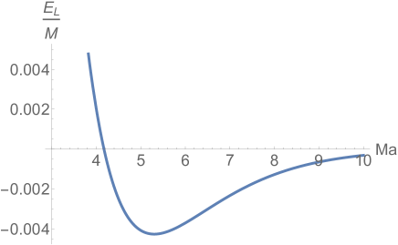
Figure 7: Crystal energy for the bcc arrangement $E_{L}/M$ versus $Ma$ as given in (58) with $\alpha_{s}=1$.

VI.1 Crystal energy

To assess the crystal contribution to the pressure at high density, we first evaluate the interaction energy for the crystal structure in Fig. 8. Consider the $L$ instanton-dyon sitting in the center of the M cell. The interaction summation within the L-lattice reads

$$2E_{L}=\sum_{n_{1},n_{2},n_{3}\neq 0}(1-(-1)^{n_{1}+n_{2}+n_{3}})V(\vec{r}_{n_{1},n_{2},n_{3}})$$ (53)

The mutual interaction between the L- and M-lattice is

$$-2E_{ML}= \sum_{n_{1},n_{2},n_{3}}(1-(-1)^{n_{1}+n_{2}+n_{3}})$$ (54)

$$\times V\left(\frac{1}{2}{\vec{r}_{111}}+\vec{r}_{n_{1},n_{2},n_{3}}\right)$$

In momentum space, these sums can be cast using the dual lattice $\vec{b}_{n}=\frac{2\pi}{a}\vec{n}$, using the identity

$$\sum_{a_{n}}e^{ip\cdot a_{n}}=\sum_{n}\delta(p-b_{n})$$ (55)

The results are

$$2E_{L}= \sum_{n}\left(V(b_{n})-V\left(b_{n}+\frac{\pi}{a}(1,1,1)\right)\right)$$

$$-2E_{ML}= \sum_{n}(-1)^{n}\left(V(b_{n})-V\left(b_{n}+\frac{\pi}{a}(1,1,1)\right)\right)$$

where we made use of

$$e^{ib_{n}\cdot\frac{r_{111}}{2}}=(-1)^{n_{1}+n_{2}+n_{3}}=(-1)^{n}$$ (57)

Both the x-space sums (53-54) and the p-space sums (LABEL:CP) can only be carried numerically. However, we note that the x-sum is converging exponentially and can be approximated by the leading contribution involving only the nearest neighbors,

$$E_{L}\equiv ME_{L}(\tilde{a})\approx M\left(6V(\tilde{a})-4V\left(\frac{\sqrt{3}\tilde{a}}{2}\right)\right)$$ (58)

with $V(x)=\frac{1}{\alpha_{s}}(-\frac{2}{x}+1)e^{-x}$ from (7) with $C_{D}=2$. Here we have set $\tilde{a}=Ma$, with $M^{2}=\frac{2n}{T}$ and $n=8\pi f$. Note that the total energy of the crystal is extensive

$$E(N,M)\approx 2NME_{L}\left(\tilde{a}\equiv Ma=\left(\frac{M^{3}V_{3}}{2N}\right)^{\frac{1}{3}}\right)$$ (59)

In Fig. 7 we show the behavior of (58) for $\alpha_{s}=1$. The bcc configuration is bound for $\tilde{a}=Ma\approx 5$, but the binding energy is very small $E_{L}/M\approx-0.004$.

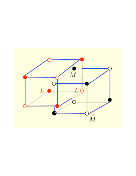
Figure 8: 3-dimensional bcc crystal composed of the instanton- and antinstanton-dyons with the lowest winding, for 2 colors.

VI.2 Disordered crystal pressure

The pressure for a disordered crystal follows from the corresponding partition function

$$\Omega_{\rm bcc}(\tilde{a})=\sum_{N}\frac{(V_{3}2\pi\tilde{f})^{4N}}{(N!)^{4}}e^{-\frac{2NM}{T}E_{L}(\tilde{a})}$$ (60)

where we used the quantum and dressed fugacity $2\pi\tilde{f}=2\pi f\sqrt{4\nu\bar{\nu}}$ from (24). In the large N-limit, the pressure ${\cal P}={{\rm ln}\Omega_{\rm bcc}}/{V_{3}}$ can be cast in the form

$$\frac{{\cal P}(\tilde{a})}{T^{3}}\approx-\frac{m^{4}}{{\tilde{a}}^{3}}E_{L}({\tilde{a}})+\frac{2m^{3}}{{\tilde{a}}^{3}}\,\left(1+{\rm ln}\left(\frac{{\tilde{a}}^{3}\sqrt{\nu\bar{\nu}}}{2m}\right)\right)$$ (61)

with $m=M/T$ (the ratio of the screening mass to the temperature). The first contribution in (61) is the crystal energy, and the second contribution is the entropy of the competing trees at large density as discussed in IVA. For large $m$ (very low temperature) the pressure is dominated by the crystal contribution, while for small $m$ (intermediate temperature) the pressure is dominated by the entropy of the trees. In Fig. 9 we show the behavior of the pressure ${\cal P}(\tilde{a})$ versus $\tilde{a}$ for $m=20$ for the center symmetric case with $\nu=\frac{1}{2}$ upper-solid-curve, while the crystal contribution is shown as the lower-solid-curve, and the tree contribution as the dashed-curve. The pressure is maximum at

$$\frac{{\cal P}_{\rm max}}{T^{3}}= \frac{m^{2}}{2}\sqrt{4\nu\bar{\nu}}e^{-\frac{m}{2}(E_{L}(\tilde{a}_{\star})-{\tilde{a}_{\star}}^{3}E_{L}^{\prime}(\tilde{a}_{\star}))}$$ (62)

$$\times\left(1-\frac{m{\tilde{a}_{\star}}^{3}}{2}E_{L}^{\prime}(\tilde{a}_{\star}\right)$$

with $\tilde{a}_{\star}$ solution to the transcendental equation

$$\frac{{\tilde{a}}^{3}_{\star}\sqrt{\nu\bar{\nu}}}{2m}=e^{\frac{m}{2}(E_{L}(\tilde{a}_{\star})-{\tilde{a}_{\star}}^{3}E_{L}^{\prime}(\tilde{a}_{\star}))}$$ (63)

If we were to assume $E_{L}$ fixed at the crystal minimum and constant as in Fig. 7, i.e $E_{L\rm min}\approx-0.004$, then (62) simplifies

$$\frac{{\cal P}_{\rm max}}{T^{3}}\rightarrow\frac{m^{2}}{2}\sqrt{4\nu\bar{\nu}}\,e^{-\frac{m}{2}{E_{L\rm min}}}$$ (64)

which is seen to interpolate between the re-summed tree contribution (33) at small $m$ (intermediate temperature) and the crystal at large $m$ (very low temperature). Due to the small binding energy of the crystal shown in Fig 7, the crystal contribution takes over only when $\frac{m}{2}$ is large or very high density (very low temperature). This is confirmed numerically. Note that in both (61) and (64) the ratio $\frac{m}{2}$ plays the role of the Coulomb factor. It is rather large with $\frac{m}{2}=500$ for the onset of the crystal.

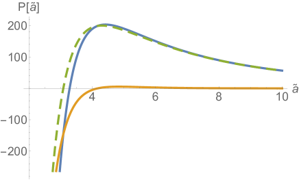
Figure 9: Pressure (61) versus $\tilde{a}$ for $m=20$ and $\nu=\frac{1}{2}$ upper-solid-curve. The separate contributions from the crystal (first term in (61)) is shown as the lower-solid-curve, and the entropy of the re-summed trees (second term in (61)) is shown as the dashed-curve.

VII Conclusions

We have provided a many-body analysis of the instanton-dyon liquid model in the center symmetric phase. The starting point of the analysis was a linearization of the moduli interactions beween like instanton-dyons $DD$ and anti-instanton-dyons ($\bar{D}\bar{D}$), followed by a cluster expansion. This re-organization of the many-body physics was shown to be captured exactly by a 3-dimensional effective theory between charged particles. A semi-classical treatment of this effective theory amounts to re-summing the tree contributions in the form of effective fugacities, while the 1-loop correction amounts to re-summing all ring or chain diagrams with effective fugacities. The tree or chain contributions are found to yield a center symmetric phase even at finite vacuum angle. They are dominant in the range $1\leq\frac{m}{2}\leq 10$.

At very low temperature or large fugacities, an even larger class of diagrams need to be re-summed. In this vein we have carried the HNC re-summation as is commonly used for dense and charged liquids, and used it to estimate the pair correlation function around the DH approximation in the dense instanton-dyon liquid. The very low temperature phase is argued to be a melted bcc crystal with strong local topological and magnetic correlations. A simple description of the thermodynamics of an ensemble composed of trees and bcc crystals show that the tree-like contributions are dominant for most temperatures, with the exception of the very low temperature regime where the crystal arrangement is more favorable owing to its very small binding. To better understand the range of validity of the present diagrammatic results, it will be important to carry a full molecular dynamics calculation for comparison. This point will be addressed next.

VIII Acknowledgements

This work was supported in part by the U.S. Department of Energy under Contract No. DE-FG-88ER40388.

IX Appendix: Molecular dynamics

(1) describes a 4-species ensemble of charged particles in 3-spatial dimensions. For fixed fugacity, the statistical ensemble described by (1) can be recovered from ensembles of classically evolved electrically and magnetically charged particles in 3-dimensions by sampling over random initial conditions. All the particles carry equal (dimensionless) mass $m_{D}=f^{\frac{2}{3}}/2\pi T^{2}$, and move classically following the Newtonian paths fixed by

$$m_{D}\,\ddot{x}_{n}= -\frac{\partial}{\partial x_{n}}\sum_{[i,\bar{i}]}\left(V(x_{i}-y_{\bar{i}})-{\rm ln}{\rm det}G[x_{i}]\right)$$

$$m_{D}\,\ddot{y}_{\bar{n}}= -\frac{\partial}{\partial y_{\bar{n}}}\sum_{[i,\bar{i}]}\left(V(x_{i}-y_{\bar{i}})-{\rm ln}{\rm det}G[y_{\bar{i}}]\right)$$ (65)

The first contribution is the Coulomb force stemming from the streamline potential, while the second contribution is the Coulomb force following from the moduli. The latter is of the form ${\rm Tr}(G^{-1}\partial_{n}G)$. It requires inverting $G$ at each time step, which may prove numerically costly for molecular dynamics (MD) simulations. It also requires that ${\rm det}\,G\neq 0$ for the inversion to be valid. For this the role of the initial conditions is important LIU (first reference).

To remedy some of these shortcomings, we recall that a linearization of the effects induced by the moduli interactions amounts to non-linear Debye-Huckel interactions between the pair $D,\bar{D}$ as captured by (10), leading simpler MD equations

$$\left(\begin{array}[]{cc}{\bf m}_{D}\,{\ddot{x}}_{D}\\ {\bf m}_{\bar{D}}\,{\ddot{x}}_{\bar{D}}\end{array}\right)=\left(\begin{array}[]{cc}-\frac{\partial}{\partial{x}_{D}}\\ -\frac{\partial}{\partial{x}_{\bar{D}}}\end{array}\right)\,\sum_{i=1,2;\underline{D}\,\underline{\bar{D}}}{V}_{i}({x}_{\underline{D}}-{x}_{\underline{\bar{D}}};\theta)$$ (70)

Here the mass ${\bf m}_{D}$ is for the pair $D=L,M$ and ${\bf m}_{\bar{D}}={\bf m}_{D}^{\dagger}$ for the pair $\bar{D}=\bar{L},\bar{M}$ at finite vacuum angle

$${\bf m}_{D}\equiv(m_{L},m_{M})=m_{D}\,e^{\frac{i\theta}{3}}\,(\nu^{\frac{2}{3}},{\bar{\nu}}^{\frac{2}{3}})$$ (71)

The potentials in (70) generalize (7) to finite vacuuum angle

$$V_{1}(r;\theta)=-V_{2}(r;\theta)=$$

$$-\frac{C_{D}}{2\alpha_{s}\,r}\left(e^{-Mre^{i\theta/4}+i\theta}+e^{-Mre^{-i\theta/4}-i\theta}\right)$$ (72)

Note that the MD analysis of (70) for $\theta\neq 0$ is more challenging as it generates complex trajectories.

References

- (1) Y. Liu, E. Shuryak and I. Zahed, Phys. Rev. D 92, no. 8, 085006 (2015); Y. Liu, E. Shuryak and I. Zahed, Phys. Rev. D 92, no. 8, 085007 (2015); Y. Liu, E. Shuryak and I. Zahed, Phys. Rev. D 94, no. 10, 105011 (2016) [arXiv:1606.07009 [hep-ph]]; Y. Liu, E. Shuryak and I. Zahed, Phys. Rev. D 94, no. 10, 105012 (2016) [arXiv:1605.07584 [hep-ph]].
- (2) Kraan-Van-Baal NPB 533 1998 T. C. Kraan and P. van Baal, Nucl. Phys. B 533, 627 (1998) [hep-th/9805168]; T. C. Kraan and P. van Baal, Phys. Lett. B 435, 389 (1998) [hep-th/9806034]; K. M. Lee and C. h. Lu, Phys. Rev. D 58, 025011 (1998) [hep-th/9802108];
- (3) D. Diakonov and V. Petrov, Phys. Rev. D 76, 056001 (2007) [arXiv:0704.3181 [hep-th]]; D. Diakonov and V. Petrov, Phys. Rev. D 76, 056001 (2007) [arXiv:0704.3181 [hep-th]]. D. Diakonov and V. Petrov, AIP Conf. Proc. 1343, 69 (2011) [arXiv:1011.5636 [hep-th]]; D. Diakonov, arXiv:1012.2296 [hep-ph].
- (4) D. Diakonov, N. Gromov, V. Petrov and S. Slizovskiy, Phys. Rev. D 70, 036003 (2004) [hep-th/0404042].
- (5) R. Larsen and E. Shuryak, arXiv:1408.6563 [hep-ph].
- (6) A. R. Zhitnitsky, hep-ph/0601057; S. Jaimungal and A. R. Zhitnitsky, hep-ph/9905540; A. Parnachev and A. R. Zhitnitsky, Phys. Rev. D 78 (2008) 125002 [arXiv:0806.1736 [hep-ph]]; A. R. Zhitnitsky, Nucl. Phys. A 921 (2014) 1 [arXiv:1308.0020 [hep-ph]].
- (7) M. Unsal and L. G. Yaffe, Phys. Rev. D 78, 065035 (2008) [arXiv:0803.0344 [hep-th]]; M. Unsal, Phys. Rev. D 80, 065001 (2009) [arXiv:0709.3269 [hep-th]]; E. Poppitz, T. Schafer and M. Unsal, JHEP 1210, 115 (2012) [arXiv:1205.0290 [hep-th]]; E. Poppitz and M. Unsal, JHEP 1107 (2011) 082 [arXiv:1105.3969 [hep-th]]; E. Poppitz, T. Schafer and M. Unsal, JHEP 1303, 087 (2013) [arXiv:1212.1238].
- (8) E. Shuryak and T. Sulejmanpasic, Phys. Rev. D 86, 036001 (2012) [arXiv:1201.5624 [hep-ph]]; E. Shuryak and T. Sulejmanpasic, Phys. Lett. B 726 (2013) 257 [arXiv:1305.0796 [hep-ph]].
- (9) P. Faccioli and E. Shuryak, Phys. Rev. D 87, no. 7, 074009 (2013) [arXiv:1301.2523 [hep-ph]].
- (10) E. Poppitz and T. Sulejmanpasic, JHEP 1309 (2013) 128 [arXiv:1307.1317 [hep-th]].
- (11) R. Larsen and E. Shuryak, Nucl. Phys. A 950, 110 (2016) [arXiv:1408.6563 [hep-ph]].
- (12) H. Frisch and J.L. Lebowitz ,The Equilibrium Theory of Classical Fluids, New York: Benjamin (1964).
- (13) M. D’Elia and F. Negro, Phys. Rev. Lett. 109, 072001 (2012) [arXiv:1205.0538 [hep-lat]].
- (14) M. Rho, S. J. Sin and I. Zahed, Phys. Lett. B 689, 23 (2010) [arXiv:0910.3774 [hep-th]]; I. Zahed, arXiv:1010.5980 [hep-ph]; P. Sutcliffe, Mod. Phys. Lett. B 29, no. 16, 1540051 (2015); V. Kaplunovsky, D. Melnikov and J. Sonnenschein, Mod. Phys. Lett. B 29, no. 16, 1540052 (2015) [arXiv:1501.04655 [hep-th]].