The UV Emission of Stars in LAMOST Survey I. Catalogs

Abstract

We present the ultraviolet magnitudes for over three million stars in the LAMOST survey, in which 2,202,116 stars are detected by $GALEX$. For 889,235 undetected stars, we develop a method to estimate their upper limit magnitudes. The distribution of (FUV $-$ NUV) shows that the color declines with increasing effective temperature for stars hotter than 7000 K in our sample, while the trend disappears for the cooler stars due to upper atmosphere emission from the regions higher than their photospheres. For stars with valid stellar parameters, we calculate the UV excesses with synthetic model spectra, and find that the (FUV $-$ NUV) vs. $R^{\prime}_{\mathrm{FUV}}$ can be fitted with a linear relation and late-type dwarfs tend to have high UV excesses. There are 87,178 and 1,498,103 stars detected more than once in the visit exposures of $GALEX$ in the FUV and NUV, respectively. We make use of the quantified photometric errors to determine statistical properties of the UV variation, including intrinsic variability and the structure function on the timescale of days. The overall occurrence of possible false positives is below 1.3% in our sample. UV absolute magnitudes are calculated for stars with valid parallaxes, which could serve as a possible reference frame in the NUV. We conclude that the colors related to UV provide good criteria to distinguish between M giants and M dwarfs, and the variability of RR Lyrae stars in our sample is stronger than that of other A and F stars.

1. Introduction

The Morgan-Keenan (MK) spectral classification system has served as the primary system for classifying stars. The classification is based on spectral continuum and features from the convection or radiative diffusion of a heated photosphere (Morgan et al., 1943). The higher regions of the stellar atmosphere (chromosphere, transition region, and corona) are often dominated by more violent non-thermal physical process mainly powered by the magnetic field. These processes related to the magnetic field could result in observable flares and starspots, and lead to discrepancy between observations and the general reference frame defined by the MK classification.

Since stellar activity is a complex phenomenon, it has many proxies, e.g., Ca II H&K lines or H_α equivalent width. Compared to spectral proxies, photometric indicators have the ability to cover much more area of the sky, and further provide a more efficient diagnosis of stellar activity (Olmedo et al., 2015). Because the UV waveband is particularly sensitive to hot plasma emission ($\sim$10${}^{4}-10^{6}$ K), the UV domain is ideal for investigating stellar activity. The availability of UV photometry as an activity indicator has been explored for Sun-like stars (Findeisen et al., 2011) and M dwarfs (Jones & West, 2016). Most of stellar activity is time dependent in the range from minutes to days (Kowalski et al., 2009; Wheatley et al., 2012). Repeated observations in the UV band provide us with an opportunity to characterize the time dependence of stellar activity, which is still poorly understood due to the previous small size of samples.

Nevertheless, data from the $Galaxy$ $Evolution$ $Explorer$ ($GALEX$; Martin et al. 2005; Morrissey et al. 2007) enable us to constrain stellar UV behavior of a large sample in both near UV (NUV; 1771$-$2831 Å) and far UV (FUV; 1344$-$1768 Å) that cover the spectral activity indicators of C II, C IV, Mg II, and Fe II. We present examples in Figure 4 in order to shown the inadequacy of photospheric models to explain the observed flux by the $GALEX$. The emission from F stars begins to exceed the flux predicted by the photospheric model (the first panel in Figure 4). The spectrum of GJ 1214 is shown in the fourth panel, in which the UV excess is strongest. This result is similar to Figure 12 in Loyd et al. (2016) that previously showed departures of the observed UV spectrum of GJ 832 from the PHOENIX model spectrum. The $GALEX$ survey provides us with an efficient path to investigate the discrepancy between observations and models for a large number of stars. $GALEX$ also presents a unique opportunity to study stellar time-domain characteristics in the UV (Gezari et al., 2013), e.g., M-dwarf flare stars (Welsh et al., 2007) and RR Lyrae stars (Welsh et al., 2005; Wheatley et al., 2008).

In this paper, we take advantage of the $GALEX$ archive data to study stellar UV emission and variation. The sample is extracted from the survey of the Large Sky Area Multi-Object Fiber Spectroscopic Telescope (LAMOST, Cui et al. 2012), which mainly aims at understanding the structure of the Milky Way (Deng et al., 2012). The survey has obtained more than four million spectra of stars from October 2011 to May 2015 (Section 2). The spectral types of these stars and accurate estimation of the stellar parameters are produced by the LAMOST standard data processing pipeline (Luo et al., 2015).

Extinction is crucial in our study, since it is about ten time higher in the UV than in the near-infrared (IR) band (Yuan et al., 2013). In Section 2, we adopt the extinction measured with a Bayesian method (Wang et al., 2016a), and the Rayleigh-Jeans Color Excess (RJCE) method (Majewski et al., 2011; Cutri et al., 2013). The infrared counterparts of our sample are cross identified with the catalog associated with the Wide-field Infrared Survey Explorer ($WISE$).

For stars observed but undetected by $GALEX$, we develop a method to estimate their upper limit magnitudes in the FUV and NUV in Section 2. In Section 3, we present the catalog and the parameters to describe UV excess and variability. We then analyze the contamination of other UV emitters and present our methods to estimate false positives. Section 4 presents the discussion and some scientific applications of our catalog. The summary and further work are given in Section 5. Throughout this paper, we adopt the extinction coefficients provided by Yuan et al. (2013) to correct Galactic extinction.

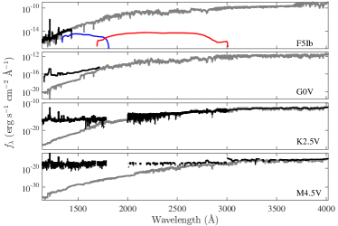
Figure 1.— Examples of the UV emission that exceeds the photospheric models. The black lines are spectra from the $HST$ Archive Data , and the gray lines are PHOENIX synthetic models. The synthetic spectra are converted to observed flux with the $V$ band magnitudes. First panel: $\alpha$ Per, $HST$ proposal 14349 by Thomas Ayres. The FUV and NUV filters of $GALEX$ are plotted in blue and red respectively. The star has strong emission lines in the FUV that are unpredicted by the model. It may have a white dwarf companion, but there is still no solid evidence (Ayres, 2017). Second panel: HD 209458, $HST$ proposal 10081 by Alfred Vidal-Madjar. Third and forth panels: HD 40307 and GJ 1214. The spectra are extracted from MUSCLES (Loyd et al., 2016) . We delete the points with flux below zero.

2. Data

2.1. LAMOST

The design of LAMOST enables it to take 4000 spectra in a single exposure to a limiting magnitude as faint as $r$ $=$ 19 at the resolution R = 1800. In 2015.05.30, LAMOST finished its third year survey (the third data release; DR3) and the all-sky coverage is $\sim$ 35%. DR3 of the LAMOST general catalog contains objects from the LAMOST pilot survey and the three-year regular survey, in all 5,755,216 objects included that are observed multiple times. Objects with unique $designation$ in the catalog are selected as unique objects. The stars of our sample are extracted from the catalog with the criteria of $class$ = STAR and $subclass$ = from O to M (Luo et al., 2015), which yields 4,010,635 stars.

The stellar parameters of $T_{\mathrm{eff}}$, log $g$, and [Fe/H] are extracted from the A, F, G and K type star catalog, which was produced by the LAMOST stellar parameter pipeline (LASP, Wu et al. 2014). The molecular indices are selected from the M star catalog.

2.2. $WISE$

We cross match the stars with the $ALLWISE$ catalogue (Cutri et al., 2013) in order to estimate the extinction with the RJCE method. We apply the following criteria to retrieve photometry in the bands of $W2$ and $H$: the match radius is set to 5″; the extended source flat (ext_flg) is set to 0; the contamination and confusion flags (cc_flags) are set to 0; and the photometric quality flag (ph_qual) is set to A (Wang et al., 2016a). Every star in our sample has an infrared counterpart in the $ALLWISE$ catalogue, but 23,388 stars do not have magnitudes in the $H$ band. We reject these stars, and there are 3,987,247 stars left.

2.3. $GALEX$

We cross match the stars to the $GALEX$ Release 6 and 7 (GR6/GR7) in order to obtain their photometry in the FUV and NUV. With the help of the Catalog Archive Server Jobs (CasJobs), nearby matching is made to the table of $PhotoObjAll$ using the following criteria: the match radius $\leq$ 5″(Gezari et al., 2013); nuv_artifact and fuv_artifact $\leq$ 1; the distance from the center of view $\leq$ 0°.55 (Jones & West, 2016); and signal-to-noise ratio of the magnitude $\geq$ 2, which yields 1,805,254 stars detected in the co-added exposures.

In order to obtain magnitudes from the visit exposures, the nearby matching is made to the table of $VisitPhotoObjAll$ with the match radius $\leq$ 5″ and the distance from the center of view $\leq$ 0°.55. The criterion of uv_artifact is not used here, since we want to select as many time-domain observations as possible. We flag the detections with uv_artifact $>$ 1 in our catalog. The result includes 2,202,116 stars detected in the co-added and/or the visit exposures. The nearest counterpart is selected for the stars with more than one counterpart within 5″ in the same exposure, and they are marked in the catalog. There are 87,178 and 1,498,103 stars detected more than once in the visit exposures in the FUV and NUV, respectively.

The observed but undetected stars are extracted from the tables of $PhotoExtract$ and $VisitPhotoExtract$, with the match radius $\leq$ 5″ and the distance from the center of view $\leq$ 0°.55. This results in an additional 889,235 stars. The density map of all the 3,091,351 stars is shown in Figure 2.

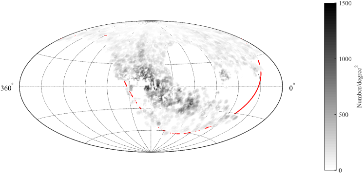
Figure 2.— The density map of stars in our catalog in Galactic coordinate. The celestial equator is shown as the red line.

2.4. Upper Limit

Gezari et al. (2013) defined the upper limit magnitude determined as a function of exposure times, and the brightness of the sky background. In their calculation, the background is a constant. However, the UV background emission, which is dominated by zodiacal light and diffuse galactic light, significantly depends on Galactic position (Murthy, 2014).

In order to calculate the position and exposure-time dependent background, we extract sources from the table of $VisitPhotoObjAll$ with the following criteria: distance from the center of view $\leq$ 0°.55; signal-to-noise ratios (S/N) $\lesssim$ 1.8 and $\lesssim$ 1.2 in the FUV and NUV. This method is similar to that used in Ansdell et al. (2015).

We average the magnitudes of these sources in the three dimensional bins: the Galactic coordinates $l$, $b$ and the exposure times. The step size of each bin is 2° and 1° for $l$ and $b$ respectively, and 10 seconds for exposure times. The magnitudes in each bin of the Galactic coordinate are then fitted with the a function similar to that in Gezari et al. (2013):

$$m_{\rm{lim}}=-2.5~{}\rm{log}(5\sqrt{\it{Sky}/T_{\rm exp}})+zp,$$ (1)

where $Sky$ is the fitted background in counts s^-1 and $zp$ values are 18.08 and 20.08 in the FUV and NUV respectively (Morrissey et al., 2007). Nearest-neighbor interpolation is used to estimate the magnitudes that are not valid in some bins of the Galactic coordinates. We present the distributions of the upper limit magnitudes on the Galactic coordinate in Figure 3. We plot the magnitudes with exposure times from 100 sec to 120 sec in the map of the detector coordinate in Figure 4, and there is no obvious correlation between the upper limit magnitudes and the distances to the detector center.

The stars with low S/N are near the detection limit of $GALEX$, and they have been used as proxies for the upper limit magnitudes. Ansdell et al. (2015) adopted an S/N of 2. We extend the S/Ns to lower values in order to come closer to the detection limit of $GALEX$, and use these stars to trace the upper limit magnitudes rather than fitting the dim bound of the UV magnitudes. We visually compare the count rate of some randomly selected sources to that of their background, and find that they are similar. The magnitudes fitted from Eq. 1 are adopted as the upper limit magnitudes for stars in the visit and the co-added exposures.

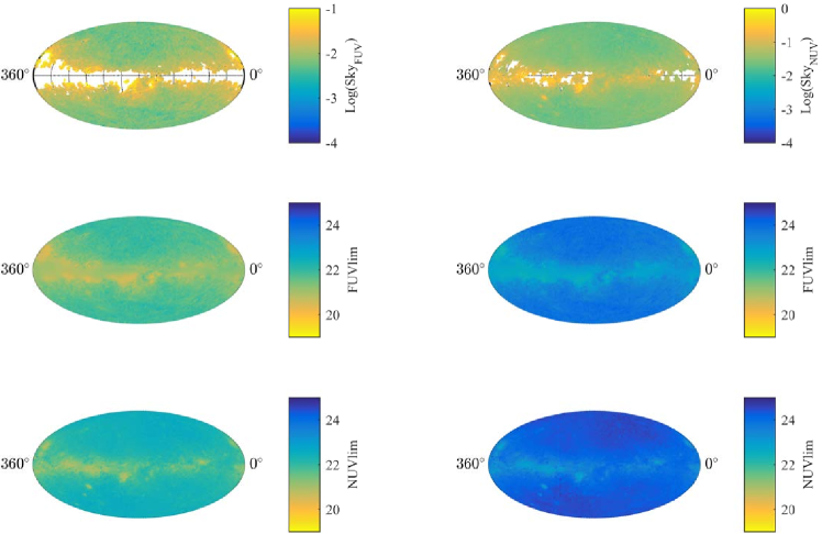
Figure 3.— The UV background and upper limit magnitudes in Galactic coordinates. Upper panels: aitoff projection of the Galactic coordinate of the fitted sky background (cts s^-1). Middle panels: the interpolated upper limit magnitudes in FUV with the exposure time from 30 to 50 sec and from 1680 to 1710 sec. Lower panels: the same as the Middle panels in NUV.

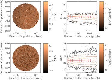
Figure 4.— The map of UV magnitudes from the detector. We accumulate all the star fields in our sample. Left panels: distributions of the sources with exposure time from 100 to 120 sec in the detector coordinate. Right panels: magnitudes as a function of the distance to the detector center. The mean value and the standard deviation for each bin is shown in red. The solid lines refer to the density contours of the magnitudes observed at a given distance from the field center.

2.5. Extinction

A novel Bayesian method developed by Burnett & Binney (2010) and Binney et al. (2014) has been used for stars in the RAVE survey, which has demonstrated the ability to obtain accurate distance and extinction. Wang et al. (2016a) measured extinction and distances using this for stars with valid stellar parameters in the first data release, and in the second data release of the LAMOST survey (Wang. J. L., private communication). They used the spectroscopic parameters $T_{\mathrm{eff}}$, [Fe/H] and log $g$, and 2MASS photometry to compute the posterior probability with the Bayesian method. They adopted a three-component prior model of the Galaxy for the distribution functions of metallicity, density, and age, in order to construct the prior probability. They then derived the probability distribution functions of parallaxes and extinctions. An introduction to this technique is given in the appendixes of Wang et al. (2016a) and Wang et al. (2016b).

For stars without valid extinction measured with Bayesian method, we use the RJCE method to estimate their extinction. This method has shown that the extinctions are reliable for most stars. The RJCE method derives the extinction by combining both the near and mid infrared. We calculate A${}_{K_{s}}$ from the equation:

$$\mathrm{A}_{K_{s}}=0.918(H-[4.5\mu\mathrm{m}]-(H-[4.5\mu\mathrm{m}])_{0}),$$ (2)

where the [4.5$\mu$m] data are the photometry of $W$2 from the $ALLWISE$ catalog (Majewski et al., 2011; Cutri et al., 2013).

Here ($H-[4.5\mu\mathrm{m}])_{0}$ is the zero point that depends on spectral types (Majewski et al., 2011). We use the BT-Cond grid (Baraffe et al., 2003; Barber et al., 2006; Allard & Freytag, 2010) of PHOENIX photospheric model (Hauschildt et al., 1999) in Theoretical Model Services (TMS) to calculate the the effective-temperature dependent zero points. Based on the calibration provided by Gray & Corbally (2009), the $subclass$ in the LAMOST catalog is used to estimate their effective temperature for stars without valid effective temperatures. The extinction provided by Schlegel et al. (1998) is adopted, if the extinction estimated from the RJCE is larger than that of the Milky Way.

Figure 5 shows the comparison between the extinction derived from the Bayesian and RJCE methods. There is no systematical deviation between the two methods statistically, but about five percent of the stars have $A_{V}$ differences larger than one. For A and K stars, extinction from the Bayesian method is higher than that from the RJCE within a discrepancy of $\Delta$A_V $\lesssim$ 0.7 mag, which is consistent with the result of Wang et al. (2016a). Extinction values from Bayesian method suffer uncertainty in the stellar parameters, if they are not well constrained in the LAMOST pipeline (Wu et al. 2011, Sec 4.4 of Luo et al. 2015). However, the Bayesian methodology offers several advantages compared to RJCE as discussed in Sale (2012). The RJCE could overestimate the extinction for stars with small $A_{V}$ (Rodrigues et al., 2014), which can be seen in the upper panel of Figure 5.

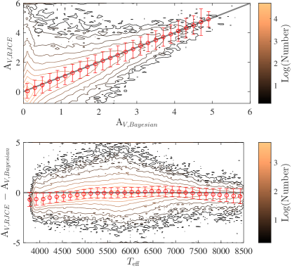
Figure 5.— The comparison between extinction derived from the Bayesian and the RJCE methods. Upper panel: the density contours of the extinction. Lower panel: the density contours of the difference as a function of effective temperature. In each panel an equal value is indicated with the solid grey lines. The solid color lines are density contours in the bin size of 0.1 magnitude of the extinction and 50 K of the effective temperature. The red circles and error bars stand for the mean values and standard deviations in the bins respectively.

3. Catalog

3.1. Magnitudes

We present the FUV and NUV counterparts from both the co-added and the visit exposures in Table 1. For stars observed but undetected by $GALEX$, we give their upper limits in the FUV and NUV. Since the co-added exposures are combined from some but not all the visit exposures, we flag the visit exposures that are combined to the listed co-added exposures.

All the magnitudes in Table 1 do not reach the limits of saturation before the extinction correction. The saturation effect is insignificant in our sample, since about 0.3% and 0.1% of the stars in the FUV and NUV reach the more conservative limits of $m_{\rm FUV}$ $<$ 12.6 and $m_{\rm NUV}$ $<$ 13.9 (Morrissey et al., 2007; Findeisen et al., 2011).

We check the distributions of exposure time in our sample. The bimodal distributions are dominated by images from the all-sky imaging survey (AIS) and the medium imaging survey (MIS).

We calculate the mean magnitudes from the average fluxes of the visit exposures, and present the colors’ distributions in Figure 6. The (FUV $-$ NUV) is not only very sensitive to the young massive stars (Kang et al., 2009), but also a useful indicator of stellar activities for low-mass stars (Welsh et al., 2006; France et al., 2016). Both K giants and dwarfs have blue (FUV $-$ NUV), probably due to the strong FUV line emission from upper atmosphere layers primarily in emission lines of C II, Si IV, and C IV (Jones & West, 2016). The stars of $T_{\mathrm{eff}}$ $\sim$ 6000 K are redder than others, forming a red valley in the HR-like diagram. On one hand, their colors are redder than earlier-type stars due to the lower effective temperatures. On the other hand, their FUV emission from upper regions of their atmosphere is weaker than that of later-type stars probably due to their weaker upper atmosphere emission.

The infrared bands, which are dominated by flux from the photosphere, are insensible to upper atmosphere emission. The very blue (FUV $-$ $J$) colors for K dwarfs are due to emission from upper atmosphere layers. The (NUV $-$ $J$) colors for the K dwarfs are not very blue because the NUV emission is mostly photospheric. The colors of (FUV $-$ $J$) and (NUV $-$ $J$) decline with increasing $T_{\mathrm{eff}}$, and dwarfs are bluer than giants. We find that the K stars with $T_{\mathrm{eff}}$ $\sim$ 4500 K, log $g$ $\sim$ 4 (the grey circles in Figure 6), are bluer than other K stars. The bluer (UV $-$ IR) colors and smaller gravities might be due to their rapid rotations (Stelzer et al., 2013) or the interactions with spectrally unresolved companions (Ansdell et al., 2015).

Table 1UV Data in Our Catalog

LID	Type	$T_{\mathrm{eff}}$	log $g$	$A_{\rm FUV}$	$A_{\rm NUV}$	fE	MJD	FUVl,v	NUVl,v	fC	FUVv	NUVv	fF	fN	FUVl	NUVl	FUV	NUV
		(K)	(cm s-2)	(mag)	(mag)		(day)	(mag)	(mag)		(mag)	(mag)			(mag)	(mag)	(mag)	(mag)
(1)	(2)	(3)	(4)	(5)	(6)	(7)	(8)	(9)	(10)	(11)	(12)	(13)	(14)	(15)	(16)	(17)	(18)	(19)
607005	F5	6603	4.22	0.37	0.55	1	3236.0179	21.26	21.90	1		17.69 $\pm$ 0.06		0	21.70	22.25		17.61 $\pm$ 0.05
							3241.4768	21.34	21.90	1		17.61 $\pm$ 0.06		0	22.98	23.54	22.28 $\pm$ 0.30	17.58 $\pm$ 0.01
							4664.2107	22.98	23.54	2	22.28 $\pm$ 0.30	17.58 $\pm$ 0.01	0	0
607006	M0	3759		0.39	0.58	0	3236.0179	21.24	21.87	0					21.67	22.22
							3241.4768	21.32	21.87	0					22.96	23.51
							4664.2107	22.96	23.51	0
607007	K0	5330	4.56	0.36	0.53	1	3236.0179	21.27	21.92	0					21.71	22.28
							3241.4768	21.35	21.92	0					23.00	23.56
							4664.2107	23.00	23.56	0
607009	G5	4866	2.50	0.40	0.59	1	3990.2005	21.80	22.22	1		21.15 $\pm$ 0.32		0	21.80	22.22		21.15 $\pm$ 0.32
607011	F9	6010		0.00	0.00	0	3236.0179	21.63	22.45	0		20.37 $\pm$ 0.31		1	22.07	22.81
							3241.4768	21.71	22.45	0		20.77 $\pm$ 0.27		1	22.07	22.81
							3990.2027	22.07	22.81	0
607013	G3	5955	4.34	0.27	0.40	1	3236.0179	21.50	22.06	0		19.06 $\pm$ 0.13		0	21.94	22.41
							3241.4768	21.58	22.06	0		19.50 $\pm$ 0.22		1	23.22	23.70		19.18 $\pm$ 0.03 ∗
							4664.2107	23.22	23.70	1		19.18 $\pm$ 0.03 ∗		0
607015	G3	5881	4.50	0.35	0.51	1	3236.0179	21.42	21.94	0		20.74 $\pm$ 0.44		1	21.86	22.30
							3241.4768	21.50	21.94	0		20.54 $\pm$ 0.33		0
607016	F5	6374	4.21	0.35	0.51	1	3990.2005	21.86	22.30	1		18.50 $\pm$ 0.07		0	21.86	22.30		18.50 $\pm$ 0.07
607018	K5	4400		0.00	0.00	0	3990.2005	22.20	22.81	0					22.20	22.81
607019	K3	4718	3.65	0.39	0.57	1	3990.2005	21.82	22.24	0					21.82	22.24
607021	K7	4104	4.75	0.18	0.26	1	3236.0179	21.46	22.19	0					21.89	22.54
							3241.4768	21.53	22.19	0					23.18	23.83
							4664.2107	23.18	23.83	0

Note. — All magnitudes are corrected for extinction. The FUV and NUV magnitudes are extracted from the catalogs of $GALEX$ GR6/GR7 and corrected for extinction. Column (1): IDs in the LAMOST catalog. Column (2): Spectral types. Column (3): Effective temperatures in the AFGK catalog or estimated with the stellar subclasses. Column (4): Surface Gravity. Column (5)-(6): Extinction in the UV. Column (7): Flags of extinction. f_E = 0, extinction calculated with the RJCE method; f_E = 1, extinction calculated with Bayesian method. Column (8): JD $-$ 2450000. Column (9)-(10): Upper limit magnitudes from visit exposures. Column (11): Flags mark the visit exposures combined into the corresponding co-added exposures for the detected stars. Column (12)-(13): Magnitudes for the stars detected from visit exposures. We mark the stars with asterisks when there are more than one counterpart within 5″in the same visit exposure. Column (14)-(15): Flags for the stars with flag_artifact $>$ 1 in the FUV and NUV, when f = 1. Column (16)-(17): Upper limit magnitudes from co-added exposures. Column (18)-(19): Magnitudes for the stars detected from co-added exposures. We mark the stars with asterisks when there are more than one counterpart within 5″in the same co-added exposure.

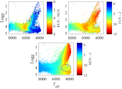
Figure 6.— The distributions of stars in the Hertzsprung-Russell-like (HR-like) diagram. The color bars represent the colors of the (FUV $-$ NUV), the (FUV $-$ $J$), and the (NUV $-$ $J$) in the bins of log $g$ and $T_{\mathrm{eff}}$. The K stars with bluer (UV $-$ IR) colors than other K stars are circled in grey.

3.2. UV Excesses

The UV excess (Eq. 3) and the normalized UV excess (Eq. 4) describe the distributions of UV flux with respect to a basal value:

$$E_{\mathrm{UV}}=m_{\mathrm{UV,obs}}-m_{\mathrm{UV,ph}},$$ (3)

$$R^{\prime}_{\mathrm{UV}}=\frac{f_{\mathrm{UV,obs}}-f_{\mathrm{UV,ph}}}{f_{\mathrm{bol}}},$$ (4)

where $f_{\mathrm{UV,obs}}$ ($m_{\mathrm{UV,obs}}$) and $f_{\mathrm{UV,ph}}$ ($m_{\mathrm{UV,ph}}$) are the observed UV flux (magnitude) and the photospheric flux (magnitude) in the same UV band. The $f_{\mathrm{bol}}$ is the bolometric flux calculated from the effective temperature (Findeisen et al., 2011; Stelzer et al., 2013).

We estimate the photospheric flux in the FUV and NUV with the BT-Cond grid. All synthetic magnitudes in the FUV, NUV, and $J$ bands are extracted with the help of TMS. We construct a theoretical grid for interpolation, and the dimensions are effective temperatures, surface gravities and metallicities. The scaling factor $(\frac{R_{*}}{d})^{2}$, the squared ratio between the stellar radius and the distance, is calculated from the (UV $-$ $J$) color predicted from the synthetic model. The scaling factor is used to convert the observed UV flux to that from the stellar surface (Stelzer et al., 2013). We only compute the $E_{\mathrm{UV}}$ and $R^{\prime}_{\mathrm{UV}}$ for stars with valid stellar parameters, and estimate their corresponding uncertainties from the errors in magnitudes, $T_{\mathrm{eff}}$, log $g$, and [Fe/H].

About 11% and 22% of the $R^{\prime}_{\mathrm{UV}}$ are below zero in the FUV and NUV, respectively. In these cases, the normalized UV excesses are insignificant and probably dominated by uncertainties in the extinction and the model interpolation. The uncertainties of the extinction are from the errors in the stellar parameters, when the extinction is given with the Bayesian method. We present stars with $R^{\prime}_{\mathrm{UV}}$ $>$ 0 in Table 2.

The color excess (FUV $-$ NUV) suffers from less uncertainties than the UV excesses, and could shed light on the stellar activity (Shkolnik, 2013; Smith et al., 2014). The normalized FUV excess as a function of (FUV $-$ NUV) is shown in Figure 7, in which the anti-correlation can be fitted with a linear relation,

$$\mathrm{Log}(\mbox{$R^{\prime}_{\mathrm{FUV}}$})=(-0.380\pm 0.001)\times(\mathrm{FUV}-\mathrm{NUV})-(4.85\pm 0.01).$$ (5)

It is suggested that the (FUV $-$ NUV) could trace the $R^{\prime}_{\mathrm{FUV}}$. The stars with stronger upper atmosphere emission have larger $R^{\prime}_{\mathrm{FUV}}$. These stars are mostly K stars with (FUV $-$ NUV) near zero. The correlation implies that such emission is more obvious in the FUV than in the NUV. Therefore, the $R^{\prime}_{\mathrm{NUV}}$ shows no obvious correlation with the (FUV $-$ NUV) in Figure 7. There is an effective temperature dependence in the $R^{\prime}_{\mathrm{FUV}}$ plot. The dependence may be due to the different FUV origination. The FUV of the early-type stars is mainly from the photospheres, while that of the late-type stars is mainly from the upper atmospheres.

We present the color-coded distributions of the UV and the normalized UV excesses in Figure 8, in which the excesses depend on $T_{\mathrm{eff}}$ and log $g$. The $E_{\mathrm{FUV}}$ increases with increasing $T_{\mathrm{eff}}$. The $E_{\mathrm{NUV}}$ has a similar distribution but with a smaller increasing level. This indicates that low mass stars have strong UV excesses, especially in the FUV.

The $R^{\prime}_{\mathrm{FUV}}$ is higher than the $R^{\prime}_{\mathrm{NUV}}$ for stars with $T_{\mathrm{eff}}$ $\lesssim$ 6000 K, since their stellar activities might be more efficient at powering the the line emission in the FUV than the continuum in the NUV (Jones & West, 2016). The $R^{\prime}_{\mathrm{UV}}$ of giants is lower than that of dwarfs, because the upper atmosphere emission of giants are buried beneath their atmospheres (Holzwarth & Schüssler, 2001; Nucci & Busso, 2014). There are some bins with average $R^{\prime}_{\mathrm{UV}}$ below zero in Figure 8, which results in the empty areas of early-type stars.

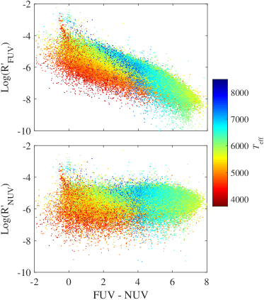
Figure 7.— The log($R^{\prime}_{\mathrm{FUV}}$) (the upper panel) and the log($R^{\prime}_{\mathrm{NUV}}$) (the lower panel) as functions of the (FUV $-$ NUV). The colored points represent the effective temperature as shown by the color bar to the right. A clear linear relation can be seen in the distribution of log($R^{\prime}_{\mathrm{FUV}}$) vs. the (FUV $-$ NUV), but there is no such relation in the NUV.

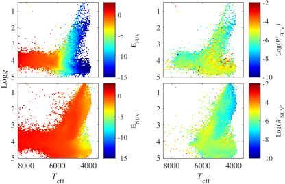
Figure 8.— The UV and the normalized UV excesses in the HR-like diagram. Left panels: the distributions of FUV and NUV excesses in the bins of $T_{\mathrm{eff}}$ and log $g$ with a bin size of 50 K and 0.05 dex. Right panels: the distributions of the normalized FUV and NUV excesses. For stars with high $T_{\mathrm{eff}}$, the normalized UV excesses are invalid due to the negative mean values in some bins.

Table 2UV Parameters in Our Catalog

LID	$E_{\mathrm{FUV}}$	$eE_{\mathrm{FUV}}$	$E_{\mathrm{NUV}}$	$eE_{\mathrm{NUV}}$	log $R^{\prime}_{\mathrm{FUV}}$	log $eR^{\prime}_{\mathrm{FUV}}$	log $R^{\prime}_{\mathrm{NUV}}$	log $eR^{\prime}_{\mathrm{NUV}}$	$\sigma_{\mathrm{int,FUV}}$	$\sigma_{\mathrm{int,NUV}}$	$S_{\mathrm{d,FUV}}$	$S_{\mathrm{d,NUV}}$
(1)	(2)	(3)	(4)	(5)	(6)	(7)	(8)	(9)	(10)	(11)	(12)	(13)
101077	$-$2.65	1.51	1.25	0.61	$-$5.37	$-$5.72						0.34
101150	$-$8.80	0.91	$-$0.54	0.49	$-$5.08	$-$5.46	$-$5.74	$-$5.86		0.52		1.54
103032	$-$0.29	0.76	$-$0.44	0.23	$-$8.07	$-$7.89	$-$5.51	$-$5.86	0.41	0.03
104056	$-$0.47	0.35	$-$0.35	0.16	$-$7.19	$-$7.39	$-$5.20	$-$5.60	0.69	0.02	0.11	0.01
106049	$-$5.74	1.16	$-$0.11	0.29	$-$5.49	$-$6.37	$-$6.11	$-$5.47	0.33	0.04	0.93	0.12

Note. — Column (1): Object IDs in the LAMOST catalog. Column (2): Excesses in the FUV. Column (3): Errors of $E_{\mathrm{FUV}}$. Column (4): Excesses in the NUV. Column (5): Errors of $E_{\mathrm{NUV}}$. Column (6): Normalized FUV Excesses. Column (7): Errors of $R^{\prime}_{\mathrm{FUV}}$. Column (8): Normalized NUV Excesses. Column (9): Errors of $R^{\prime}_{\mathrm{NUV}}$. Column (10): Intrinsic variabilities in the FUV. Column (11): Intrinsic variabilities in the NUV. Column (12): Structure functions on timescales of days in the FUV. Column (13): Structure functions on timescales of days in the NUV.

3.3. Variability Statistics

The rms scatter has been used to describe the intrinsic variability in optical and UV bands (Sesar et al., 2007; Gezari et al., 2013),

$$\sigma_{\mathrm{int}}=\sqrt{\Sigma^{2}-\langle\xi\rangle^{2}},~{}\mathrm{where}~{}\Sigma=\sqrt{\frac{1}{n-1}\sum^{n}_{i=1}(m_{i}-\langle{m}\rangle)^{2}}.$$ (6)

In order to estimate the mean photometric error $\langle\xi\rangle$, we extract over six million objects in the FUV and NUV bands. The mean photometric error depends on both the magnitude and the exposure time in Figure 9. We construct a two dimensional grid with bin size of ${\Delta}m$ = 0.5 magnitude and $\Delta$log(ExpT) = 0.1 second.

We then obtain mean photometric error with the interpolation, and calculate the rms scatter $\sigma_{\rm{int}}$ of the stars detected in at least two visit exposures. It yields 46,022 and 700,039 stars with available $\sigma_{\rm{int}}$ in the FUV and NUV, respectively. The distributions of $\sigma_{\rm{int}}$ are presented in the left panels of Figure 10. The intrinsic variability declines with the increase of $T_{\mathrm{eff}}$, implying that late-type stars tend to have strong variabilities. The $\sigma_{\rm int}$ values in the FUV are generally larger than those in the NUV, probably due to the higher amplitudes of light curves in the shorter wavelength (Wheatley et al., 2012).

Another parameter to characterize the variability is the structure function (see di Clemente et al. 1996 for details),

$$V(\Delta{t})=\sqrt{\frac{\pi}{2}\langle|\Delta{m_{ij}}|\rangle^{2}_{\Delta{t}}-\langle\sigma^{2}_{i}+\sigma^{2}_{j}\rangle},$$ (7)

where brackets stand for averages for all pairs of points on the light curve of an individual source with $i$ $<$ $j$, $\Delta{m_{ij}}=m(t+\Delta{t})-m(t)$ and $t_{j}-t_{i}=\Delta{t}$. We calculate the structure functions on the time scale of days, $S_{\rm{d}}$, from the characteristic-time bins of $V(\Delta{t})$. The $S_{\rm{d}}$ is defined as the maximum value of the structure function evaluated for $\Delta{t_{2d}}=2\pm 0.5$ d, $\Delta{t_{4d}}=4\pm 0.5$ d, $\Delta{t_{6d}}=6\pm 0.5$ d, $\Delta{t_{8d}}=8\pm 0.5$ d (Gezari et al., 2013). This value is also presented in Table 2. The distributions of $S_{\rm{d}}$ are shown in the right panels of Figure 10. The distributions of $\sigma_{\rm{int}}$ and $S_{\rm{d}}$ are similar. The stars with lower $T_{\mathrm{eff}}$ have higher variabilities, which might be naturally explained by the strong upper atmosphere emission of late-type stars.

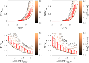
Figure 9.— The uncertainties as functions of the magnitudes and the exposure times in the FUV (left panels) and the NUV (right panels). The solid color lines are density contours with a bin size of 0.5 magnitudes, 0.01 uncertainties, and 0.1 seconds in the log scale. The red points and error bars stand for the mean values and standard deviations in the bins respectively.

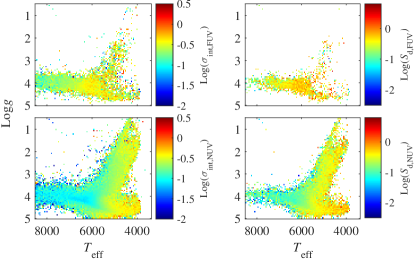
Figure 10.— The parameters of variations in the HR-like diagram. Left panels: the distributions of the intrinsic variations in the bins of log $g$ and $T_{\mathrm{eff}}$. Right panels: same as the left panels but for the structure functions, $S_{\rm d}$ in the FUV and NUV.

3.4. False Positives

The stars can appear UV-luminous for some reasons not related to their upper atmosphere emission or photospheric radiation. These cases are so called false positives, which are false matched background active galactic nuclei (AGNs) within $\sim$5″. Another kind of possible false positive is binaries composed of non-degenerate stars and white dwarfs. These binaries are unresolved by spectra from the LAMOST facility. The wrongly selected UV counterpart should also be considered as false positives, when there are more than one counterpart within 5″ in the same exposure.

We estimate the probability of false positives from background AGNs by matching false-star positions within a random arcminute of their true positions with the $GALEX$ archive data (Jones & West, 2016). It yields about a 0.14% chance of matching for given a random position, and about 0.25% for our sample given over 55% of the LAMOST stars are detected in $GALEX$.

The catalog of Rebassa-Mansergas et al. (2013) is used to select the potential white dwarf main-sequence (WDMS) binaries in our sample. We follow the same procedure described in Section 2 to find the UV counterparts of these WDMS binaries. We find that the combination of UV and IR could separate WDMS binaries, since they cluster at FUV $-$ NUV $\sim$ 0 and W1 $-$ W2 $\sim$ 0.14 in Figure 11. There are 17,428 stars in our sample, $\sim$ 0.56%, located inside the density contour of two per bin, which are potential WDMS-binary candidates unresolved by LAMOST (Table 3).

There are 13,845 stars having more than one counterpart within 5″ in the same co-added or visit exposures. If they are all wrongly selected as UV counterparts, the occurrence of false positives is 0.45%. The overall occurrence of these false positives is below 1.3% in our sample.

Table 3The WDMS Candidates in Our Catalog

LID	FUV	NUV	W1	W2
(1)	(2)	(3)	(4)	(5)
102042	21.56 $\pm$ 0.13	20.64 $\pm$ 0.08	13.02 $\pm$ 0.02	12.92 $\pm$ 0.03
102173	21.54 $\pm$ 0.44	21.86 $\pm$ 0.19	14.57 $\pm$ 0.03	14.62 $\pm$ 0.06
103165	23.26 $\pm$ 0.30	23.82 $\pm$ 0.36	14.25 $\pm$ 0.03	14.13 $\pm$ 0.04
104029	21.66 $\pm$ 0.31	21.74 $\pm$ 0.18	13.32 $\pm$ 0.03	13.36 $\pm$ 0.03
104250	21.34 $\pm$ 0.06	21.06 $\pm$ 0.02	12.64 $\pm$ 0.02	12.60 $\pm$ 0.03
106053	23.04 $\pm$ 0.44	21.31 $\pm$ 0.01	14.65 $\pm$ 0.03	14.61 $\pm$ 0.07
106057	22.13 $\pm$ 0.43	22.56 $\pm$ 0.31	13.27 $\pm$ 0.03	13.14 $\pm$ 0.03
106063	22.32 $\pm$ 0.19	22.67 $\pm$ 0.07	14.45 $\pm$ 0.03	14.50 $\pm$ 0.06
106241	22.32 $\pm$ 0.19	20.85 $\pm$ 0.02	15.89 $\pm$ 0.06	15.73 $\pm$ 0.16
107224	21.06 $\pm$ 0.46	20.13 $\pm$ 0.07	13.24 $\pm$ 0.02	13.25 $\pm$ 0.03

Note. — All magnitudes are corrected for extinction. Column (1): Object IDs in the LAMOST catalog. Column (2): Mean magnitudes calculated from all the magnitudes in the visit exposures in the FUV. Column (3): The same as Column (2) in NUV. Column (4): Magnitudes in the $W1$. Column (5): Magnitudes in the $W2$.

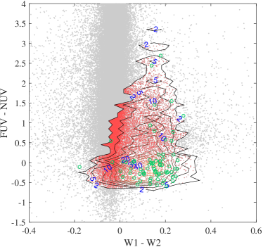
Figure 11.— The diagram of (FUV $-$ NUV) vs. (W1 $-$ W2) for the stars in our sample and the WDMS binaries. The solid lines are density contours in the bin size of 0.1 magnitude for WDMS binaries of Rebassa-Mansergas et al. (2013). The densities are marked as blue numbers along the contours. The WDMS binaries of Ren et al. (2014) are shown as green circles. The stars in our sample located inside the density contour of two per bin are shown as red points, and others are shown in grey.

4. Discussion

4.1. Colors and Comparison with SDSS

We present color distributions in Figure 12. The (FUV $-$ NUV) declines with increasing effective temperature for stars with $T_{\mathrm{eff}}$ $>$ 7000 K, because their UV fluxes are dominated by radiation from stellar photospheres. This trend disappears and the UV color distribution becomes dispersive for stars with $T_{\mathrm{eff}}$ $\sim$ 6000 K, since their UV colors from upper atmosphere emission probably became comparable to photospheric UV colors. Some inactive G stars follow the colors predicted by the model, while other active stars have blue excesses. These active G stars might be either in active close binaries or young single stars (Smith et al., 2014).

For stars later than G, the color distributions exhibit remarkably blue excesses, because of the additional bluer UV emission from the upper regions of atmosphere. The UV colors of these stars are (FUV $-$ NUV) $\sim$ 1, similar to the blue peak in Smith et al. (2014), which might imply the general colors of the stellar active regions.

When integrate the distributions of all stars with different types, we also detect the bimodal distribution of (FUV $-$ NUV) in our sample, similar to Smith et al. (2011). The bimodal distribution is perhaps due to the two sub-populations, the UV red stars having weak activities and mid effective temperatures, and the UV blue stars having strong activities or high effective temperatures (Smith et al., 2014).

The peaks of the distributions are anti-correlated to effective temperatures in the figures of (FUV $-$ $J$) and (NUV $-$ $J$), but we can see obvious blue excesses for the stars with $T_{\mathrm{eff}}$ $\lesssim$ 6000 K and $T_{\mathrm{eff}}$ $\lesssim$ 5500 K in the two figures, respectively. This implies the beginning at which the radiation from upper regions of the atmosphere dominates the UV flux. For stars with higher effective temperatures, the UV fluxes are mainly from stellar photospheres, where the UV-IR colors depend on the effective temperatures rather than the upper atmosphere emission.

There are some late A stars redder than the colors predicted by theoretical models in the distribution of (NUV $-$ $J$). The nature of the bias is still unclear, which might indicate some deviation between observation and theoretical templates for the radiation from stellar photospheres, or amount to potential spectrally unresolved companion stars with slightly lower effective temperature than primary stars.

We cross match the stars having valid stellar parameters in our catalog with the SDSS stars processed through the SEGUE Stellar Parameter Pipeline (SSPP, Lee et al. 2008a,Lee et al. 2008b), in order to check the difference in the effective temperatures derived from two independent pipelines. In Figure 12, there is no obvious systematical deviation in the color distributions. We can conclude that the distributions of the colors associated with UV are independent in the stellar parameter pipelines, and indicate intrinsic properties of our sample. Here we do not cross identify with APOGEE stars, since they are mainly giants with effective temperatures in the range from 4000 to 5500 K .

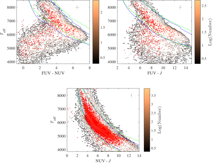
Figure 12.— The effective temperature as functions of the (FUV $-$ NUV), (FUV $-$ $J$) and (NUV $-$ $J$) for stars in our catalog (contours) and the matched stars processed through the SSPP in the SDSS archive (red points). The blue solid lines stand for the color ranges from PHOENIX photospheric models, and those from ATLAS9 models (Castelli et al., 1997) are shown in green for comparison. The average errors are presented as grey crosses in the upper right corners.

4.2. Scientific Applications

Because of its large size and homogeneous nature, this catalog not only provides a wealth of information for the study of upper atmosphere emission, but also enables a time-domain exploration in the UV. In this section, we would like to discuss some scientific applications of the catalog.

4.2.1 A Passible UV Reference Frame

The MK spectral classification sets the general reference frame for stars on physical parameters, and further plays a critical role in identification of the truly peculiar stars which do not fit comfortably into the frame (Gray & Corbally, 2009, 2014). However, the reference frame is poorly constrained in the UV band due to small samples of stellar emission from upper regions of atmospheres. Using this large catalog, we could present a possible UV reference frame based on radiation from all regions of stellar photospheres.

We calculate the absolute magnitudes for stars with valid parallaxes (Wang et al., 2016a), and average the fluxes in each bin of $T_{\mathrm{eff}}$ and log $g$ (left panels of Figure 13). The UV absolute magnitude declines with the increase of the effective temperature, which is similar to the results of Shkolnik (2013), while the standard deviation is larger in the FUV than the NUV for stars with $T_{\mathrm{eff}}$ $\lesssim$ 6000 K. Such standard deviation is probably due to their strong intrinsic variability, as shown in the upper two panels in Figure10. Because of the small standard deviation and homogeneity in the stellar parameters, the NUV absolute magnitudes could be used as a possible reference frame to calibrate the stellar NUV emission. Such NUV emission includes the stellar radiation not only from the photosphere but also the upper regions of the atmosphere.

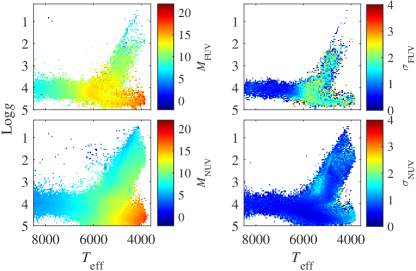
Figure 13.— The UV absolute magnitudes in an HR-like diagram. Left panels: the distributions of absolute magnitudes in the FUV and NUV. Right panels: the standard deviation in the bins of $T_{\mathrm{eff}}$ and log $g$.

4.2.2 Colors of Giant and Dwarf Stars

Giant stars, owing to their high luminosities, are popular tracers of substructures in the Milky Way, and help us address important questions, e.g., the size of our Galaxy (Bochanski et al., 2014), the shape of the dark matter halo (Piffl et al., 2014), substructures in the outer Galactic halo (Sheffield et al., 2014), the metallicity distribution (Hayden et al., 2015), etc.

We use the criterion provided by Ciardi et al. (2011) to separate giants from dwarfs. Neither the UV involved colors (Figure 14) nor the UV excesses can provide a good separation between giants and dwarfs in our sample. The distribution of dwarfs exhibits a clear ’$\Lambda$’ shape. The stars in the right branch are mainly K dwarfs, which overlap with the giants. The UV involved colors could separate the stars with $T_{\mathrm{eff}}$ $\sim$ 6000 K, located in the red valley in Figure 6, from other stars with higher temperatures or stronger upper atmosphere emission. UV and IR photometry based methods cannot provide a good separation, but some spectra related methods could distinguish giants, such as spectral line features (Liu et al., 2014).

However, the color of the (NUV $-$ $J$) can separate M giants from M dwarfs in Figure 15. Here we use a robust linear separation, the lowest density of the stars in the diagram of molecular-band indices in Figure 16 (Zhong et al., 2015). The upper atmosphere emission of giant star is weaker than those of dwarfs, and the colors constructed by both UV and IR bands could provide a good statistical separation.

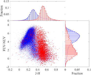
Figure 14.— The color-color diagram for the giants (red) and dwarfs (blue) in our sample, and a clear $\Lambda$-shape distribution can be seen for dwarfs. The upper and right panels show histograms of the colors.

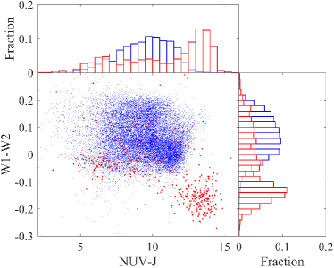
Figure 15.— The color-color diagram for the M giants (red) and M dwarfs (blue) in our sample. The upper and right panels show the histograms of the colors.

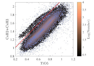
Figure 16.— The diagram of the CaH2$+$CaH3 versus TiO5 for M stars in our sample (light blue dots). The density contours are the sample in the M stars catalog, and the separation between giants and dwarfs is shown as the red line. The M stars above the red line are giants.

4.2.3 RR Lyrae Stars

RR Lyr Stars are pulsating periodic horizontal-branch variables with great variation in the UV in the range of 2$-$5 mag (Wheatley et al., 2012), making them more likely to be detected in the UV. They are thus popular tracers of Galactic structures, the halo (Sesar et al., 2010) and streams (Drake et al., 2013).

We cross match the RR Lyr stars in Drake et al. (2013) and Abbas et al. (2014) with our sample, and plot them over the A and F stars in Figure 17. The UV counterparts of RR Lyr stars are concentrated in the region of high $S_{\rm d}$ and $\sigma_{\rm{int,NUV}}$, and have a bluer color of (FUV $-$ $J$) than other A and F stars. In Figure 18, we plot the light curve of an RR Lyr star with LID $=$ 254809148 as an example. The amplitude of the UV light curve is higher than that in the optical band by a factor of 2 (Sesar et al., 2010).

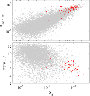
Figure 17.— The properties of RR Lyrae stars in our sample. Upper panel: the diagram of $\sigma_{\rm int}$ versus $S_{\rm d}$ of A and F stars in our sample (the gray dots), and the matched RR Lyrae stars of Drake et al. (2013) and Abbas et al. (2014) (the red dots). Lower panel: the (FUV $-$ $J$) as a function of the $S_{\rm d}$.

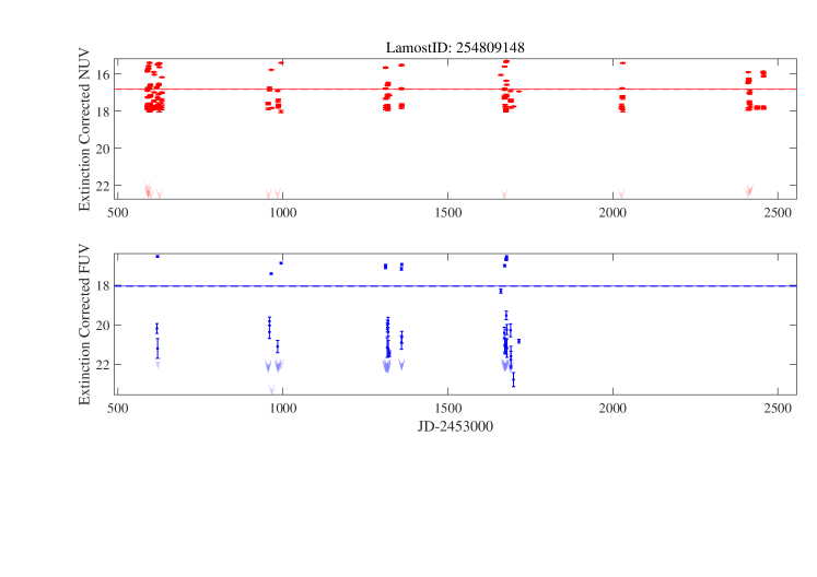
Figure 18.— The light curves of an RR Lyrae star in our sample in the FUV (blue) and NUV (red). The error bars are magnitudes in the visit exposures, and the arrows are undetected upper limit magnitude in the visit exposures. The solid and hashed lines are mean magnitudes and their errors respectively.

5. Summary and Further Work

We provide a catalog of over three millon $GALEX$-observed stars, and the parameters to quantify stellar activity and variability, based on well estimated background and extinction, a newly developed method on upper limit magnitudes, spectral properties from the LAMOST, and time-resolved photometry in the FUV and NUV. This includes 2,202,116 detected and 889,235 undetected stars. The occurrence of possible false positives is below 1.3% in our sample, and the candidates of spectrally unresolved WDMS are selected from the UV involved color-color diagram.

The emission from regions beyond the stellar photosphere could result in the discrepancy between observed UV minus IR colors and those predicted by theoretical photospheric models. We quantify such discrepancy by the UV and normalized UV excesses, and find that they both decline with increasing effective temperatures, and the late-type dwarfs tend to have high excesses. Similar to other studies, the normalized UV excess suffers from large systematic uncertainties in the photosphere contribution, especially for stars with high effective temperatures. The systematic uncertainties of these stars may be from errors in the extinction and the model interpolation. We present a linear relation between the (FUV $-$ NUV) and the $R^{\prime}_{\mathrm{FUV}}$. The UV color as a proxy of the FUV excess is recommended when the stellar parameter is unavailable. The distributions of the parameterized variation in the HR-like diagram shows that the effective temperature declines with increasing variability.

We also provide the absolute magnitudes in an HR-like diagram, which could serve as a possible reference frame in the NUV. With the UV involved colors, the M giants and M dwarfs could be well separated, but other giants and dwarfs cannot be distinguished with colors or UV excesses. We find that the RR Lyrae stars, strong UV emitters, have stronger variation than most A and F stars in our sample.

The stellar parameters are available for a portion of late A, F, G and K stars in our catalog, which are applied to estimate the UV and normalized UV excesses. In order to investigate the excesses for stars with other spectral types, we could introduce other catalogs, e.g., the further data released of the LAMOST Spectroscopic Survey of the Galactic Anticentre (LSS-GAC, Yuan et al. 2015) in which the parameters are derived from LSP3 (Xiang et al., 2015), and a more complete version of M stars from LAMOST (Zhong et al., 2015) in which a template matching technique is used. The UV emission of B, A and M stars will be characterized in detail in our further studies.

We are also going to study the stars located in the grey circle in Figure 6, with time-resolved spectra in order to check their binarity. The further mid-resolution spectra in LAMOST survey may shed light on the rotations of these stars.

References

- Abbas et al. (2014) Abbas, M. A., Grebel, E. K., Martin, N. F., et al. 2014, MNRAS, 441, 1230
- Allard & Freytag (2010) Allard, F., & Freytag, B. 2010, Highlights of Astronomy, 15, 756
- Ansdell et al. (2015) Ansdell, M., Gaidos, E., Mann, A. W., et al. 2015, ApJ, 798, 41
- Ayres (2017) Ayres, T. R. 2017, ApJ, 837, 14
- Baraffe et al. (2003) Baraffe, I., Chabrier, G., Barman, T. S., Allard, F., & Hauschildt, P. H. 2003, A&A, 402, 701
- Barber et al. (2006) Barber, R. J., Tennyson, J., Harris, G. J., & Tolchenov, R. N. 2006, MNRAS, 368, 1087
- Binney et al. (2014) Binney, J., Burnett, B., Kordopatis, G., et al. 2014, MNRAS, 437, 351
- Bochanski et al. (2014) Bochanski, J. J., Willman, B., Caldwell, N., et al. 2014, ApJ, 790, L5
- Burnett & Binney (2010) Burnett, B., & Binney, J. 2010, MNRAS, 407, 339
- Castelli et al. (1997) Castelli, F., Gratton, R. G., & Kurucz, R. L. 1997, A&A, 318, 841
- Ciardi et al. (2011) Ciardi, D. R., von Braun, K., Bryden, G., et al. 2011, AJ, 141, 108
- Cui et al. (2012) Cui, X.-Q., Zhao, Y.-H., Chu, Y.-Q., et al. 2012, Research in Astronomy and Astrophysics, 12, 1197
- Cutri et al. (2013) Cutri, R. M., Wright, E. L., Conrow, T., et al. 2013, Explanatory Supplement to the AllWISE Data Release Products, by R. M. Cutri et al.
- Deng et al. (2012) Deng, L.-C., Newberg, H. J., Liu, C., et al. 2012, Research in Astronomy and Astrophysics, 12, 735
- di Clemente et al. (1996) di Clemente, A., Giallongo, E., Natali, G., Trevese, D., & Vagnetti, F. 1996, ApJ, 463, 466
- Drake et al. (2013) Drake, A. J., Catelan, M., Djorgovski, S. G., et al. 2013, ApJ, 765, 154
- France et al. (2016) France, K., Parke Loyd, R. O., Youngblood, A., et al. 2016, ApJ, 820, 89
- Findeisen et al. (2011) Findeisen, K., Hillenbrand, L., & Soderblom, D. 2011, AJ, 142, 23
- Gezari et al. (2013) Gezari, S., Martin, D. C., Forster, K., et al. 2013, ApJ, 766, 60
- Gray & Corbally (2009) Gray, R. O., & Corbally, C., J. 2009, Stellar Spectral Classification by Richard O. Gray and Christopher J. Corbally. Princeton University Press
- Gray & Corbally (2014) Gray, R. O., & Corbally, C. J. 2014, AJ, 147, 80
- Hauschildt et al. (1999) Hauschildt, P. H., Allard, F., & Baron, E. 1999, ApJ, 512, 377
- Hayden et al. (2015) Hayden, M. R., Bovy, J., Holtzman, J. A., et al. 2015, ApJ, 808, 132
- Holzwarth & Schüssler (2001) Holzwarth, V., & Schüssler, M. 2001, A&A, 377, 251
- Jones & West (2016) Jones, D. O., & West, A. A. 2016, ApJ, 817, 1
- Kang et al. (2009) Kang, Y., Bianchi, L., & Rey, S.-C. 2009, ApJ, 703, 614
- Kowalski et al. (2009) Kowalski, A. F., Hawley, S. L., Hilton, E. J., et al. 2009, AJ, 138, 633
- Lee et al. (2008a) Lee, Y. S., Beers, T. C., Sivarani, T., et al. 2008a, AJ, 136, 2022
- Lee et al. (2008b) Lee, Y. S., Beers, T. C., Sivarani, T., et al. 2008b, AJ, 136, 2050
- Liu et al. (2014) Liu, C., Deng, L.-C., Carlin, J. L., et al. 2014, ApJ, 790, 110
- Loyd et al. (2016) Loyd, R. O. P., France, K., Youngblood, A., et al. 2016, ApJ, 824, 102
- Luo et al. (2015) Luo, A.-L., Zhao, Y.-H., Zhao, G., et al. 2015, Research in Astronomy and Astrophysics, 15, 1095
- Majewski et al. (2011) Majewski, S. R., Zasowski, G., & Nidever, D. L. 2011, ApJ, 739, 25
- Martin et al. (2005) Martin, D. C., Fanson, J., Schiminovich, D., et al. 2005, ApJ, 619, L1
- Morgan et al. (1943) Morgan, W. W., Keenan, P. C., & Kellman, E. 1943, An Atlas of Stellar Spectra (Chicago, IL: Univ. of Chicago Press)
- Morrissey et al. (2007) Morrissey, P., Conrow, T., Barlow, T. A., et al. 2007, ApJS, 173, 682
- Murthy (2014) Murthy, J. 2014, ApJS, 213, 32
- Nucci & Busso (2014) Nucci, M. C., & Busso, M. 2014, ApJ, 787, 141
- Olmedo et al. (2015) Olmedo, M., Lloyd, J., Mamajek, E. E., et al. 2015, ApJ, 813, 100
- Piffl et al. (2014) Piffl, T., Binney, J., McMillan, P. J., et al. 2014, MNRAS, 445, 3133
- Rebassa-Mansergas et al. (2013) Rebassa-Mansergas, A., Agurto-Gangas, C., Schreiber, M. R., Gänsicke, B. T., & Koester, D. 2013, MNRAS, 433, 3398
- Ren et al. (2014) Ren, J. J., Rebassa-Mansergas, A., Luo, A. L., et al. 2014, A&A, 570, A107
- Rodrigues et al. (2014) Rodrigues, T. S., Girardi, L., Miglio, A., et al. 2014, MNRAS, 445, 2758
- Sale (2012) Sale, S. E. 2012, MNRAS, 427, 2119
- Schlegel et al. (1998) Schlegel, D. J., Finkbeiner, D. P., & Davis, M. 1998, ApJ, 500, 525
- Sesar et al. (2007) Sesar, B., Ivezić, Ž., Lupton, R. H., et al. 2007, AJ, 134, 2236
- Sesar et al. (2010) Sesar, B., Ivezić, Ž., Grammer, S. H., et al. 2010, ApJ, 708, 717
- Sesar et al. (2010) Sesar, B., Vivas, A. K., Duffau, S., & Ivezić, Ž. 2010, ApJ, 717, 133
- Sheffield et al. (2014) Sheffield, A. A., Johnston, K. V., Majewski, S. R., et al. 2014, ApJ, 793, 62
- Shkolnik (2013) Shkolnik, E. L. 2013, ApJ, 766, 9
- Smith et al. (2011) Smith, M., Shiao, B., & Kepler 2011, Bulletin of the American Astronomical Society, 43, 140.16
- Smith et al. (2014) Smith, M. A., Bianchi, L., & Shiao, B. 2014, AJ, 147, 159
- Stelzer et al. (2013) Stelzer, B., Marino, A., Micela, G., López-Santiago, J., & Liefke, C. 2013, MNRAS, 431, 2063
- Wang et al. (2016a) Wang, J., Shi, J., Zhao, Y., et al. 2016, MNRAS, 456, 672
- Wang et al. (2016b) Wang, J., Shi, J., Pan, K., et al. 2016, MNRAS, 460, 3179
- Welsh et al. (2005) Welsh, B. Y., Wheatley, J. M., Heafield, K., et al. 2005, AJ, 130, 825
- Welsh et al. (2006) Welsh, B. Y., Wheatley, J., Browne, S. E., et al. 2006, A&A, 458, 921
- Welsh et al. (2007) Welsh, B. Y., Wheatley, J. M., Seibert, M., et al. 2007, ApJS, 173, 673
- Wheatley et al. (2008) Wheatley, J. M., Welsh, B. Y., & Browne, S. E. 2008, AJ, 136, 259
- Wheatley et al. (2012) Wheatley, J., Welsh, B. Y., & Browne, S. E. 2012, PASP, 124, 552
- Wu et al. (2011) Wu, Y., Luo, A.-L., Li, H.-N., et al. 2011, Research in Astronomy and Astrophysics, 11, 924
- Wu et al. (2014) Wu, Y., Du, B., Luo, A.L., et al. 2014, IAUS, 306, 340
- Xiang et al. (2015) Xiang, M. S., Liu, X. W., Yuan, H. B., et al. 2015, MNRAS, 448, 822
- Yuan et al. (2013) Yuan, H. B., Liu, X. W., & Xiang, M. S. 2013, MNRAS, 430, 2188
- Yuan et al. (2015) Yuan, H.-B., Liu, X.-W., Huo, Z.-Y., et al. 2015, MNRAS, 448, 855
- Zhong et al. (2015) Zhong, J., Lépine, S., Li, J., et al. 2015, Research in Astronomy and Astrophysics, 15, 1154