Unfair and Anomalous Evolutionary Dynamics from Fluctuating Payoffs

Abstract

Evolution occurs in populations of reproducing individuals. Reproduction depends on the payoff a strategy receives. The payoff depends on the environment that may change over time, on intrinsic uncertainties, and on other sources of randomness. These temporal variations in the payoffs can affect which traits evolve. Understanding evolutionary game dynamics that are affected by varying payoffs remains difficult. Here we study the impact of arbitrary amplitudes and covariances of temporally varying payoffs on the dynamics. The evolutionary dynamics may be ”unfair“, meaning that, on average, two coexisting strategies may persistently receive different payoffs. This mechanism can induce an anomalous coexistence of cooperators and defectors in the Prisoner’s Dilemma, and an unexpected selection reversal in the Hawk-Dove game.

How species interact depends on the environment and is thus often uncertain or subject to ongoing variations. Traditional game theory has assumed constant payoff structures. Here, we demonstrate by independent methods that the dynamics of averaged payoff values does not well approximate the dynamics of fluctuating payoff values. We show that payoff fluctuations induce qualitative changes in the dynamics. For instance, a Prisoner’s Dilemma with payoff fluctuations may have the evolutionary dynamics of a Hawk-Dove game with constant payoff values. As a consequence, cooperators can coexist with defectors – without any further cooperation maintaining mechanism such as kin or group selection Traulsen2006b ; Lehmann2007 , reciprocity Nowak2006five , or spatial structures Nowak1992 .
First of all, how environmental fluctuations and payoff stochasticities affect the evolution of interacting species depends on the time scales. If the fluctuations are much faster than reproduction, adaptation reaches a stationary state where species are adapted to living in a rapidly fluctuating environment. If the fluctuations are much slower than the generation time (e. g. ice ages or geomagnetic field reversals), adaptation quickly reaches a stationary state which slowly drifts to follow the fluctuation. Ultimately challenging is the case when the fluctuations and reproduction are at a similar pace such that adaptation is continuously following the environmental changes. Here, we show that such states are subject to noise-induced transitions. Noise-induced transitions have been studied in dynamical systems, where the most prominent models study the effects of additive noise Broeck1997 ; Toral2011 ; Horsthemke1984 . In dynamical systems, both additive and multiplicative noise can lead to an array of anomalous noise-induced effects such as stochastic resonance Gammaitoni1998 and the creation of stable states Lipshtat2006 ; Biancalani2015 . We wish to investigate the consequences of multiplicative noise in evolutionary game theory that have not been systematically studied yet.

A number of studies used stochastic models of population extinction to analyze the impact of environmental stochasticity on the extinction risk of small and large populations Leigh1981 ; Lande1993 ; Foley1994 . Particular attention has been spent on how the species’ mean time to extinction depends on a small randomly varying growth rate Ovaskainen2010 , and on the autocorrelation of the environmental noise Schreiber2010 ; Morales1999 ; Heino2000 ; Wilmers2007 ; Schwager2006 ; Heino2003 ; Ruokolainen2009 ; Greenman2005 ; Kamenev2008 . Likewise in evolutionary game theory, the question of how fixation, i. e. the transition to the survival of only one species, depends on environmental stochasticity attracted a lot of attention Nowak2004 ; Traulsen2006 ; Altrock2009 ; Assaf2013 ; Ashcroft2014 ; Houchmandzadeh2015 . Recently, how the fixation depends on environmental stochasticity was also studied in the case of multi-player games Baron2016 .

As opposed to these efforts, we will focus on the impact of payoff fluctuations on the stationary states.
Environmental fluctuations have been integrated in models for evolutionary games in different ways, including fluctuating reproduction rates Foster1990 ; Fudenberg1992 ; Hofbauer2009 ; Traulsen2004 , selection strength Assaf2013 and population size Houchmandzadeh2012 ; Houchmandzadeh2015 ; Huang2015 ; Gokhale2016 ; Constable2016 . We integrate environmental fluctuations as varying payoff values to study situations in which the environmental fluctuations affect the way the species interact. Thereby we assume that all individuals experience the same environment, meaning that the payoff values vary with time but not between individuals.

We explore the landscape of dynamical changes of evolutionary games induced by such fluctuating payoffs. We consider both deterministic (e. g. seasonal) as well as stochastic fluctuations with varying intensities and correlations. For a realistic description it is necessary to also include intrinsic noise in finite populations Lande1993 ; Taylor2004 ; Nowak2004 ; Traulsen2006 . However, we aim to reveal phenomena that were unknown so far because they were hidden by the idealized assumption of constant payoffs. Therefore we isolate the effects of fluctuating payoffs from the diverse effects of intrinsic noise in finite populations by studying the replicator equation, which describes the evolution of strategies in infinite populations, and the Moran process Moran1958random for finite but large populations.

Anomalous evolutionarily stable states

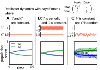
Figure 1: Selection reversal in a Hawk-Dove game with constant, periodic and random payoff. (A) describes a traditional Hawk-Dove game. The population starts at $x_{1}=x_{2}=0.5$ (50 % Hawks, 50% Doves) and converges to an evolutionarily stable state where $x_{1}>x_{2}$. Periodically (B) or randomly fluctuating payoffs (C) shift the evolutionarily stable state such that $x_{1}<x_{2}$.

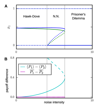
Figure 2: Fluctuations transform a Hawk-Dove game into a Prisoner’s Dilemma and cause “unfair” stable coexistence. (A) Shown is the anomalous stationary state (solid line: stable, dashed line: unstable) of the fraction of cooperators $x_{1}$ as a function of the noise intensity. Due to alternating payoff values the stationary states consist of two periodic points (green and blue). With increasing intensity, the dynamical structure of a Hawk-Dove game first changes to a game without analog in traditional games (N.N.) and finally to a Prisoner’s Dilemma game. (B) The difference of the averaged payoffs received by the two players corresponding to the stationary states of coexistence in A. In the arithmetic mean the received payoffs are unfair. In the geometric mean they are equal, as predicted by Eq. (4).

Multiplicative growth is a common model that underlies both population and evolutionary dynamics. In the simple case of time-discrete exponential growth, the population number $n$ is described by $n_{t+1}=rn_{t}$. Depending on the growth rate $r$, the population will diverge ($r>1$), remain constant ($r=1$) or decay ($0\leq r<1$). However, a time-dependent growth rate $r_{t}$ can lead to intricate results. As an example, compare a growth rate that is switching between $1$ and $1.1$ with a growth rate that is switching between $0.6$ and $1.5$. Both have the same arithmetic average that is greater than one, but the population will diverge in the first case because $1\cdot 1.1=1.1$ and decay in the second case because $0.6\cdot 1.5=0.9$. In general, the long-term growth is determined by the geometric mean of the growth rate $\bar{r}$, and the population will diverge if $\bar{r}>1$, remain constant if $\bar{r}=1$ and decay if $0\leq\bar{r}<1$. Like in this example, multiplicative noise has generally a net-negative effect on growth in the long-term Lewontin1969 ; Peters2011 ; Peters2013 .
Models of evolutionary game theory are more complex but share the same underlying property, which leads to noise-induced non-ergodic behavior.

In the classical Hawk-Dove game two birds meet and compete for a shareable resource $V$, the positive payoff. If a Hawk meets a Dove the Hawk alone gets the resource, if two Doves meet they share the resource and if two Hawks meet they fight for the resource, which costs energy and implies the risk of getting injured, formalized by a negative payoff $-C$. Since 50% of the Hawks win and 50% of the Hawks loose a fight, the average payoff of a Hawk meeting a Hawk in the limit of an infinite population is $\frac{V-0}{2}+\frac{0-C}{2}=\frac{V-C}{2}$.
Fig. 1 (A) shows that for $V=1$ and $C=1.5$ the time-discrete replicator dynamics leads to an evolutionarily stable state in which a larger population of Hawks coexists with a smaller population of Doves. However, in a changing environment the payoff matrix will not be constant. For example, the abundance of the food resource may change periodically with the seasons, or the risk of death caused by an injury may depend on the presence of predators. Fig. 1 (B) and (C) show how the evolutionarily stable state can change if $V$ or $C$ fluctuate such that their averages are still the same as in (A). Similar to the aforementioned example with the exponential growth process, the noise has a net-negative effect on the long-term growth of the strategies in replicator dynamics, too. Due to the specific structure of the Hawk-Dove game payoff matrix, the negative effect of the noise of both $V$ and $C$ is stronger for the population of Hawks than for the Doves, such that with sufficient noise the Doves dominate the population in the evolutionarily stationary state. Next, we show that these anomalous effects are generic for evolutionary games.

In evolutionary game theory the interactions are usually formalized in a payoff function, which specifies the reward from the interaction with another player that is received by a given individual. In the simplest case, a game with two strategies is determined by a payoff matrix $M$ with $2\times 2$ matrix elements. We describe the state of the population as $\mathbf{x}$ ($\sum{x_{i}}=1$), where $x_{i}\geq 0$ is the fraction of players with strategy $i\in\{1,2\}$. Players with strategy $i$ receive the payoff $P_{i}=(M\mathbf{x})_{i}+b$, where the background fitness $b$ ensures that the payoff is positive. The assumption that species that receive a higher payoff reproduce faster can be formalized by the replicator equation, which is used here in its time-discrete form Taylor1978

$$x^{(t+1)}_{i}=x_{i}^{(t)}\cdot r_{i}(\mathbf{x}^{(t)},M),$$ (1)

with $$r_{i}(\mathbf{x}^{(t)},M)=\frac{(M\mathbf{x}^{(t)})_{i}+b}{\mathbf{x}^{(t)T}M\mathbf{x}^{(t)}+b}=\frac{P_{i}}{\langle P\rangle}$$ (2)

and the average payoff of the population $\langle P\rangle=x_{1}P_{1}+x_{2}P_{2}$.
Following Smith Smith1982 , “a population is said to be in an ‘evolutionarily stable state’ [henceforth ESS] if its genetic composition is restored by selection after a disturbance, provided the disturbance is not too large.” Hence the ESS describe the long-term behavior of the system and are stable stationary states of Eq. (1). For a constant payoff matrix $M$, the stationary states $\mathbf{x}^{*}$ satisfy $r_{i}(\mathbf{x}^{*},M)=1$. If two species coexist, $r_{1}(\mathbf{x}^{*},M)=r_{2}(\mathbf{x}^{*},M)$ implies that both receive the same payoff $P_{1}=P_{2}=\langle P\rangle$, as otherwise the species with the higher payoff would move the system away from this state due to faster growth.
Now consider continuously changing payoffs with finite means. The stationary states $\mathbf{x}^{*}(t)$ are solutions of

$$\overline{r_{i}(\mathbf{x}^{*},M)}:=\lim_{T\rightarrow\infty}\left(\prod_{t=0}^{T-1}r_{i}(\mathbf{x}^{*}(t),M^{(t)})\right)^{\frac{1}{T}}=1\text{,}$$ (3)

where $M^{(t)}$ is the time-dependent payoff matrix. Equation (3) defines the geometric average, indicated henceforth by the bar. If the payoff matrix changes deterministically with period $T$ a stationary state is a periodic function $\mathbf{x}^{*}(t)=\mathbf{x}^{*}(t+T)$; if it changes randomly a stationary state is a random function $\mathbf{x}^{*}(t)$ with distribution $\rho^{*}(\mathbf{x})$. But how does one calculate the stationary states for periodically and randomly changing payoff matrices? In contrast to normal ESS the stationary states are not solutions of $\langle P_{1}\rangle=\langle P_{2}\rangle$, where $\langle P_{i}\rangle:=\lim_{T\rightarrow\infty}\frac{1}{T}\sum_{t=0}^{T-1}\left(M^{(t)}\mathbf{x}^{*}(t)\right)_{i}$ is the arithmetic time average of the received payoff.

Equation (3) implies that ${\overline{r_{1}(\mathbf{x}^{*},M)}=\overline{r_{2}(\mathbf{x}^{*},M)}}=1$, and, using Eq. (2), that

$$\overline{P_{1}}=\overline{P_{2}}.$$ (4)

If the fluctuations are small, we can approximate the geometric mean by $\overline{P_{i}}=\langle P_{i}\rangle-\frac{\sigma_{i}^{2}}{2\langle P_{i}\rangle}+\mathcal{O}(\sigma_{i}^{4})$ (see Supplementary Material S1), where $\sigma_{i}^{2}=\text{Var}[P_{i}]$. Using this approximation in Eq. (4) yields

$$\langle P_{1}\rangle-\frac{\sigma_{1}^{2}}{2\langle P_{1}\rangle}=\langle P_{2}\rangle-\frac{\sigma_{2}^{2}}{2\langle P_{2}\rangle}$$ (5)

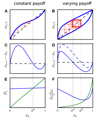
Figure S1: Evolutionarily stable states for constant and periodic payoff. An evolutionary game with a time-constant payoff matrix (left) compared with a game with a time-varying payoff matrix (right) to exemplify the “unfair” stationary states. The former payoff matrix represents a Hawk-Dove game and the latter an alternating payoff matrix which has the same time-average as the constant Hawk-Dove game. (A) and (B) show the dynamics of the two games as a Verhulst diagram with an example trajectory in red. The two blue curves in (B) correspond to even and odd time points, with the anomalous stationary states at $x_{n}^{\star}$ and $x_{n}^{\dagger}$. (C) and (D) show the difference of the state one (C) or two (D) time steps later and the current state. The zero crossings of these lines are the positions of the fixed point and the periodic points. (E) and (F) show the payoff of species 1 (blue) and species 2 (green). In (E), the equilibrium is at the same position as the fixed point. In (F), species 1 receives a higher time-averaged payoff than species 2 at both periodic points.

Equation (5) shows that $\langle P_{1}\rangle$ and $\langle P_{2}\rangle$ are generally different, which is why we call these stationary states unfair. It includes the case of constant payoff values as a special case. Figure 2 (A) illustrates how payoff fluctuations may change the evolutionary dynamics and thereby transform one game into another game. Figure 2 (B) shows how the arithmetic and the geometric average of the payoffs the two species receive deviate (see also Supplementary Fig. S1).

Deterministic payoff fluctuations

We first consider deterministic payoff fluctuations under the replicator equation (Eq. (1)). To find the stationary state $\mathbf{x}^{*}$ we solve Eq. (3). We assume that $M^{(t)}$ is a sequence with period $T$. Consequently, the stationary state $\mathbf{x}^{*(t)}$ is periodic as well and $P(\mathbf{x},M)=\frac{1}{T}\sum_{t=0}^{T}\delta(\mathbf{x}-\mathbf{x}^{*(t)})\delta(M-M^{(t)})$. Equation (3) reduces to

$$\overline{r_{i}(\mathbf{x}^{*},M)}=\left(\prod_{t=t^{\prime}}^{t^{\prime}+T}r_{i}\left(\mathbf{x}^{*(t)},M^{(t)}\right)\right)^{\frac{1}{T}} =1.$$ (6)

Note that Eq. (6) has only one free variable because if one periodic point $\mathbf{x}^{*(t^{\prime})}$ is given, the others are determined by Eq. (1).
As an illustrative example, assume an alternating payoff matrix $M^{(t)}=\overline{M}+(-1)^{t}\sigma\tilde{M}$. Then $\mathbf{x}^{*(t)}=\overline{\mathbf{x}}^{*}+(-1)^{t}\Delta\mathbf{x}^{*}$ has the same form and can be found by solving Eq. (6), which reduces to

$$\overline{r_{i}(\mathbf{x}^{*},M)}=\sqrt{r_{i}(\mathbf{x}^{*(t)},M^{(t)})\cdot r_{i}(\mathbf{x}^{*(t+1)},M^{(t+1)})}=1.$$ (7)

Figure 2 shows the stationary states of a game with the payoff function

$$M^{(t)}=\begin{pmatrix}1.1&0.8\\ 2&0\end{pmatrix}+(-1)^{t}\sigma\begin{pmatrix}-0.33&1\\ 1&0\end{pmatrix}$$ (8)

For $\sigma=0$ this is a Hawk-Dove game. For small $\sigma$, in fact, the stationary states predicted by Eq. (7) slightly deviate from the ESS of the Hawk-Dove game. There is a first bifurcation at $\sigma\approx 4.07$, from one stable stationary state (solid curves) to two. At $\sigma\approx 6.4$ there is a second bifurcation where the first branch, the stable coexistence, disappears. The bifurcation behavior induces a pronounced hysteresis effect. Ergodicity breaking causes anomalous player’s payoff expectations as shown in Fig. 2 (B). The arithmetic mean of the payoff difference that the players receive also shows a pronounced hysteresis effect. For the geometric mean, as predicted by Eq. (4), this effect is absent.
More generally, fluctuations can even change the number, the positions and the stability of stationary states and the dynamics can be structurally very different from the dynamics of games with constant payoffs, as shown in Fig. 3. In Fig. 3 (A) large fluctuations induce the onset of cooperation for the Prisoner’s dilemma as it is effectively transformed to a Hawk-Dove game with stable coexistence. Figures 3 (B), (C) and (D) show how increasing fluctuations successively transform three other classical games either into different classical games or into games without classical analogs (denoted at “N.N.”).

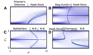
Figure 3: Evolutionarily stable states with increasing fluctuation intensity. Stable and unstable states (solid and dashed lines) $x_{1}^{*}(\sigma)$ for games with alternating payoff fluctuations (blue and green are the two periodic points). The payoff matrices are $M^{(t)}=[3,1,4,2]+(-1)^{t}\sigma[0,0,0,1]$ in (A), $M^{(t)}=[4,1,3,2]+(-1)^{t}\sigma[1,0,0,1]$ in (B), $M^{(t)}=[2,3,4,1]+(-1)^{t}\sigma[0,1.3,1.3,0]$ in (C) and $M^{(t)}=[3,2,4,1]+(-1)^{t}\sigma[-0.75,1,-2,1]$ in (D). In each example the background fitness is $b=10$. The names of the games are identified using criteria described in the Supplementary Material S3.
For the same games but stochastic instead of alternating noise, the background shows the average of three stationary distributions resulting from the initial distributions $\delta(x)$, $\delta(x-0.5)$ and $\delta(x-1)$.

In the Supplementary Material S2, we show how anomalous stationary states arise from (correlated) stochastic payoffs, which is mathematically more involving but shows similar effects as from deterministic fluctuations.

Discussion

Payoff noise in evolutionary dynamics is multiplicative and as such causes ergodicity breaking. The consequences have intricate effects on the coevolution of strategies. Depending on the details of the system, on the intensity of the fluctuations and even on their covariance, ergodicity breaking leads to shifting the payoffs out of equilibrium, shifting the stationary states and thereby to fundamental structural changes of the dynamics.
In evolutionary games with constant payoffs, the condition for stable coexistence is that all species have equal growth rates. With fluctuating payoffs this condition generalizes to equal time-averaged growth rates, which typically are different from ensemble averages in non-ergodic systems. When one naively replaces fluctuating payoffs with their average values, the ensemble averages of the growth rates are recovered but these averages do not correctly predict the dynamics.

Games with fluctuating payoffs require a novel classification that cannot be based on payoff ranking schemes. We developed a classification that primarily considers the dynamical structure (Supplementary Material S3). Our classification for evolutionary games may be applied to evolutionary games where the payoff structure cannot be described by a simple payoff matrix, or when other modifications affect the dynamical structure. Examples include complex interactions of microbes such as cooperating and free-riding yeast cells, where the payoff is a nonlinear function of the densities Gore2009 .
Payoff fluctuations can cause two strategies that coexist in an evolutionarily stable state to receive different time-averaged payoffs. However, these “unfair” stable states are not mutationally stable. Mutations, in fact, would turn the “unfair” stable state into a meta-game, where the beneficiary aims to increase and the victim aims to escape the unfairness. Strategies of this meta-game could be tuning the adaptation or reproduction rate according to the environmental fluctuation Traulsen2004 . Phenotypic plasticity Pigliucci2005 and bet-hedging Bergstrom2014 may reduce the necessity to adapt at all.
In general, the understanding of evolutionary games in fluctuating environments may be particularly relevant to understanding and controlling microbiological systems. Examples for evolutionary games in microbiology are diverse and include yeast cells Gore2009 , viruses Turner2003 and bacteria Kirkup2004 ; Griffin2004 ; Dugatkin2005 ; Yurtsev2013 . Because many of these microbes evolve in natural and artificial environments which are fluctuating, the presented effects are relevant in biotechnology and healthcare. A stable coexistence of antibiotic-sensitive bacteria with antibiotic-degrading bacteria has been proven to be a stable state of a Hawk-Dove-like game Dugatkin2005 ; Yurtsev2013 if the antibiotic concentration is constantly above the concentration which the sensitive bacteria could tolerate alone. Our framework qualitatively describes the competitive interplay of bacteria strains in a fluctuating environment, for instance, in a patient who is given a daily dose of antibiotic instead of a continuous infusion.
Simple experimental settings can directly demonstrate the consequence of non-ergodic anomalous long-term behaviors in microbiological systems. Expected shifts and bifurcations in the stationary states of strategies for two strains, or species, competing for resources (and survival) suggest to study the (co)evolutionary dynamics for a fluctuating control parameter $c$ that, e.g., switches between two levels in a square-wave fashion, $c=[c^{+},c^{-},c^{+},c^{-},c^{+},\ldots]$, where $c^{+}=c+A$ and $c^{-}=c-A$. For increasing fluctuation amplitude $A$, the stationary state is expected to shift, or to change discontinuously, both as a result of ergodicity breaking. The strongest effect is expected for fluctuations that are of the same time scale as the reproduction period of the model organisms. However, quantitative predictions require much more specific model systems deVos2017 .

To conclude, caution is advised when predictions are based on averaged observables, in particular, averaged payoffs structures. Our framework predicts anomalous stationary states as a generic result of ergodicity breaking in evolutionary dynamics that depend on the amplitude and covariance of the fluctuations.

We thank Christoph Hauert for comments on the manuscript. F.S. acknowledges funding through the International Max Planck Research School (IMPRS) “Physics of Biological and Complex Systems”. J.N. acknowledges support from the ETH Risk Center (grant no. RC SP 08-15) and from SNF (grant The Anatomy of Systemic Financial Risk, no. 162776).

Supplementary Information

Appendix S1 Approximation of the geometric mean

Let $X$ be a random variable with $\text{E}[X]=\mu$, $\text{E}[(X-\text{E}[X])^{2}]=\sigma^{2}$ and $\text{E}[(X-\text{E}[X])^{3}]=0$. We can write the geometric mean of $X$ as

$$\overline{X}=\overline{\mu+\sigma Y}=\lim_{T\to\infty}\prod_{t=0}^{T}(\mu+\sigma y_{t})^{\frac{1}{T}},$$ (S1)

where $Y$ is a random variable with $\text{E}[Y]=0$, $\text{E}[(Y-\text{E}[Y])^{2}]=1$ and $\text{E}[(Y-\text{E}[Y])^{3}]=0$. Now we have the geometric mean as a function of $\sigma$ and can write the Taylor series of $\overline{X}(\sigma)$ at $\sigma=0$,

$$\overline{X} =\overline{X}(0)+\frac{\mathrm{d}\overline{X}}{\mathrm{d}\sigma}(0)\sigma+\frac{\mathrm{d}^{2}\overline{X}}{\mathrm{d}\sigma^{2}}(0)\frac{\sigma^{2}}{2}+\frac{\mathrm{d}^{3}\overline{X}}{\mathrm{d}\sigma^{3}}(0)\frac{\sigma^{3}}{6}+\mathcal{O}(\sigma^{4})$$ (S2)

$$=\mu-\frac{\sigma^{2}}{2\mu}+\mathcal{O}(\sigma^{4})$$ (S3)

Appendix S2 Stochastic payoff fluctuations

S2.1 Replicator equation

How do anomalous stationary states arise from stochastic payoffs? To avoid unnecessary technicalities, we consider the case of two strategies, in which the state is fully described by a scalar $x=x_{1}$ (because $x_{2}=1-x_{1}$) and the payoff $M=\mathbf{Y}=\begin{pmatrix}Y_{1}&Y_{2}\\ Y_{3}&Y_{4}\end{pmatrix}$ is a random matrix, where $Y_{j}$ have probability density functions $P_{Y_{j}}(y_{j})$, mean $E(Y_{j})=\mu_{j}$ and variance $\text{Var}(Y_{j})=\sigma_{j}^{2}$. In short, we can write the replicator equation as

$$X^{(t+1)}=f(X^{(t)},\mathbf{Y})$$ (S4)

with $f(x,\mathbf{y})=x^{(t)}\cdot\frac{(y^{(t)}\mathbf{x}^{(t)})_{1}+b}{\mathbf{x}^{(t)T}\mathbf{y}^{(t)}\mathbf{x}^{(t)}+b}$. In order to get a function which is injective with respect to $\mathbf{Y}$ we define a new function

$$f^{\prime}(X^{(t)},\mathbf{Y})=\begin{pmatrix}f(X^{(t)},\mathbf{Y})\\ Y_{2}\\ Y_{3}\\ Y_{4}\end{pmatrix}$$ (S5)

This function is invertible, hence we can derive the joint probability $P_{f^{\prime}}(x^{(t+1)},y_{2},y_{3},y_{4})$ from the joint probability $P_{\mathbf{Y}}(y_{1},y_{2},y_{3},y_{4})=P(y_{1})P(y_{2})P(y_{3})P(y_{4})$ by changing variables,

$$P_{f^{\prime}}(x^{(t+1)},y_{2},y_{3},y_{4})=\left|\text{det}[Df^{\prime-1}]\right|P_{\mathbf{Y}}(f^{\prime-1})$$ (S6)

The stochastic kernel can be derived by marginalizing over $y_{2}$, $y_{3}$ and $y_{4}$.

$$K(x^{(t+1)}|x^{(t)})=\int\int\int P_{f^{\prime}}(x^{(t+1)},y_{2},y_{3},y_{4})\times$$

$$P_{Y_{2}}(y_{2})P_{Y_{3}}(y_{3})P_{Y_{4}}(y_{4})\mathrm{d}y_{2}\mathrm{d}y_{3}\mathrm{d}y_{4}$$ (S7)

The Chapman-Kolmogorov equation gives the time evolution of the probability density

$$P^{(t)}_{X}(x)=\int_{0}^{1}\mathrm{d}x^{\prime}P^{(t-1)}_{X}(x^{\prime})K(x|x^{\prime}),$$ (S8)

To ease the numerical evaluation we use the look-ahead-estimator Stachurski2008

$$P^{(t)}_{X}(x)=\frac{1}{n}\sum_{l=1}^{n}K(x|s_{l}^{t-1})$$ (S9)

where $\{s_{l}\}$ is a sample of size $n$ drawn from $P^{(t-1)}_{X}(x)$. Starting with an arbitrary initial distribution $P^{(1)}_{X}(x)$ and successively applying Eq. (S9) converges to a stationary distribution $\rho^{*}(x)=P^{(\infty)}_{X}(x)$ of the stochastically driven replicator dynamics.
The background in Fig. 3 shows that the stationary distributions, apart from the expected broadening, follow the behavior of the stable states derived for analogous deterministic fluctuations.

We now demonstrate that the type of the distribution has only little effect on the stationary states. As an example we use a game with the payoff function

$$M^{(t)}=\begin{pmatrix}1&0.5\\ 2&0\end{pmatrix}+X\begin{pmatrix}0&0\\ 1&0\end{pmatrix}$$ (S10)

with the background fitness $b=10$. Note that the zero-noise case of this game resembles a Hawk-Dove game. Fig. S2 shows the stationary distributions $\rho^{*}(x_{1})$ of the replicator dynamics and the Moran process, where $X$ is either a uniform, discrete, normal distributed random variable or alternations, each with variance $\sigma=2$. The higher moments of the noise distribution have little effect on the resulting stationary distribution.

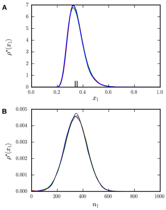
Figure S2: Stationary distributions of replicator dynamics (A) and Moran model (B) for different noise sources ($\sigma=2$). Red: Uniform distributed, green: discrete distributed, blue: normal distributed, black: alternating noise.

S2.2 Moran processes

Employment of Moran processes has been shown to be imperative for the mathematical understanding of stochastic evolutionary game theory. Despite being conceptionally very different from replicator dynamics, Moran processes are affected by payoff fluctuations in a similar way.
Consider a Moran process with population size $N$ and payoff matrix $M=\mathbf{Y}=\begin{pmatrix}Y_{1}&Y_{2}\\ Y_{3}&Y_{4}\end{pmatrix}$, where $Y_{j}$ are uncorrelated random variables with probability density functions $P_{Y_{j}}(y_{j})$ (note that also a deterministically changing payoff with period $T=2$ can be mapped to this formulation). If the number of individuals playing strategy 1 is $i$, the expected payoff received by an individual playing strategy 1 or 2 is

$$p_{1}(t) =\frac{1}{N-1}\left[y_{1}(t)(i-1)+y_{2}(t)(N-i)\right]$$ (S11)

$$p_{2}(t) =\frac{1}{N-1}\left[y_{3}(t)i+y_{4}(N-i-1)\right]$$ (S12)

With selection strength $w$ the fitness of each strategy $k=1,2$ reads

$$f_{k}(t)=1-w+wp_{k}.$$ (S13)

The (non-zero) transition probabilities are

$$T(i|i+1)= \int\frac{f_{1}(\mathbf{Y})i(N-i)}{[f_{1}(\mathbf{Y})i+f_{2}(\mathbf{Y})(N-i)]N}P_{\mathbf{Y}}(\mathbf{y})\mathrm{d}\mathbf{y}$$

$$+g(i/N)$$ (S14)

$$T(i|i-1)= \int\frac{f_{2}(\mathbf{Y})i(N-i)}{[f_{1}(\mathbf{Y})i+f_{2}(\mathbf{Y})(N-i)]N}P_{\mathbf{Y}}(\mathbf{y})\mathrm{d}\mathbf{y}$$

$$+g(1-i/N)$$ (S15)

where we use the abbreviation $P_{\mathbf{Y}}(\mathbf{y})\mathrm{d}\mathbf{y}=P_{Y_{1}}(y_{1})P_{Y_{2}}(y_{2})P_{Y_{3}}(y_{3})P_{Y_{4}}(y_{4})\mathrm{d}y_{1}\mathrm{d}y_{2}\mathrm{d}y_{3}\mathrm{d}y_{4}$ and add $g(x)=\delta(x)$ to achieve reflecting boundaries. The explicit form of the transition probabilities allows to calculate the anomalous stationary state as the solution of the Fokker-Planck equation for the Moran process Traulsen2006a

$$\partial_{t}\rho(x,t)=-\partial_{x}\left[a(x)\rho(x,t)\right]+\frac{1}{2}\partial_{x}^{2}\left[b^{2}(x)\rho(x,t)\right]$$ (S16)

which reads

$$\rho^{*}(x)=\mathcal{N}\exp{\left(\int_{0}^{x}\Gamma(x^{\prime})\mathrm{d}x^{\prime}\right)}$$ (S17)

for

$$\mathcal{N}=\int_{0}^{1}\exp{\left(\int_{0}^{x}\Gamma(x^{\prime})\mathrm{d}x^{\prime}\right)}\mathrm{d}x,$$ (S18)

and

$$\Gamma(x)=\frac{1}{b(x)}\left(2a(x)-\frac{\mathrm{d}b}{\mathrm{d}x}(x)\right),$$ (S19)

where $a(x)=T(x|x+1/N)-T(x|x-1/N)$, $b(x)=\sqrt{\left(T(x|x+1/N)+T(x|x-1/N)\right)/N}$, and $x=\frac{i}{N}$.
Figure S3 shows for an example how the stationary distributions, predicted by Eq. (S17), change with increasing fluctuation intensities compared to stationary distributions of the simulated Moran model.

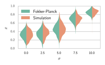
Figure S3: Anomalous stationary distributions of the Moran model: Theory and simulation. Stationary distributions calculated by the Fokker-Planck equation and measured stationary distributions using a simulation of the Moran model in comparison. The payoff matrix is $M^{(t)}=[6,5.5,7,5]+X^{t}\sigma[0,0,1,0]$, with $X^{t}$ randomly switching between $+1$ and $-1$. The population size is $N=1000$.

S2.3 Correlated fluctuations

Payoff values are not necessarily statistically independent from each other, as for example the payoff values $M_{11}$ and $M_{12}$ of the Hawk-Dove game in Fig. 1. Thus, it is informative to study the effects of covariation. Consider the general case of a game specified by the payoff matrix $M=\begin{pmatrix}Y_{1}&Y_{2}\\ Y_{3}&Y_{4}\end{pmatrix}$. In order to show the impact of the correlations, we keep the intensity of the fluctuations equal and constant, $\sigma_{Y_{1}}=\sigma_{Y_{2}}=\sigma_{Y_{3}}=\sigma_{Y_{4}}=\text{const}$. The correlations between $Y_{1}$, $Y_{2}$, $Y_{3}$ and $Y_{4}$ are specified by six independent correlation coefficients on which the resulting stationary states depend in a nonlinear way. For simplicity, Fig. S4 shows only the isolated impact of each pairwise correlation keeping the others zero.

This shows that in addition to intensities, the anomalous stationary states are crucially determined by the correlation of the fluctuations. Yet, we can show analytically that there is a special case ($\text{corr}(Y_{1},Y_{3})=\text{corr}(Y_{2},Y_{4})=1$) for which the stationary state becomes completely independent of the fluctuation intensities. Assume that $\mathbf{x}^{*}$ is the stationary state of a game with constant payoff matrix $M_{0}$, such that $r(\mathbf{x}^{*},M_{0})=1$. If we add noise with correlation coefficient $1$ between column values,

$$M(t)=M_{0}+\tilde{M}(t)=\begin{pmatrix}a&b\\ c&d\end{pmatrix}+\begin{pmatrix}f_{1}(t)&f_{2}(t)\\ f_{1}(t)&f_{2}(t)\end{pmatrix},$$ (S20)

then

$$r\left(\mathbf{x}^{*},M_{0}+\tilde{M}(t)\right)=\frac{(M_{0}\mathbf{x}^{*})_{i}+(\tilde{M}(t)\mathbf{x}^{*})_{i}+b}{\mathbf{x}^{*T}M_{0}\mathbf{x}^{*}+\mathbf{x}^{*T}\tilde{M}(t)\mathbf{x}^{*}+b}$$ (S21)

$$=\frac{(M_{0}\mathbf{x}^{*})_{i}+(f_{1}(t)x_{1}^{*}+f_{2}(t)x_{2}^{*})+b}{\mathbf{x}^{*T}M_{0}\mathbf{x}^{*}+(f_{1}(t)x_{1}^{*}+f_{2}(t)x_{2}^{*})+b}=1$$ (S22)

where the second step uses $x_{1}^{2}+x_{1}x_{2}=x_{1}$ and $x_{2}^{2}+x_{1}x_{2}=x_{2}$ and the last step uses $(M_{0}\mathbf{x}^{*})_{i}=\mathbf{x}^{*T}M_{0}\mathbf{x}^{*}$ following from the assumption. Consequently, in this case the stationary state does not depend on the noise intensity.

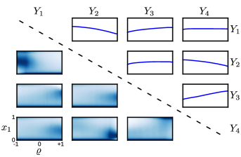
Figure S4: Impact of correlations. Periodic points $x^{\star}$ (upper part) and stationary distributions (lower part) for fluctuations with equal intensity ($\sigma=5$) but different correlation coefficients $\varrho$. Each plot shows the impact of the correlation between two entries of the payoff matrix while keeping all other correlations zero.

Appendix S3 Classification of games with payoff fluctuations

S3.1 Generalized criteria

A symmetric game defined by a constant $2\times 2$ payoff matrix can be classified as one out of 12 game classes with distinct dynamical structures, e. g. Prisoner’s Dilemma, Hawk-Dove game, etc. This traditional classification is based on the rank of the four values in the payoff matrix, see middle column in table S1. The name of a game allows a more intuitive understanding than the position in the four dimensional payoff space. However, this classification cannot be applied to time-varying payoff matrices because the ranks may be time-dependent. Therefore we propose a classification for evolutionary games based on three characteristics: (1) the dynamics of the evolutionary game (the number of stationary states and their stability), (2) the type of social interaction (how the payoff differs between stationary states for one player compared to the other player) and (3) the effect on the community (how the total payoff of player one and two differs between stationary states). The classification scheme and its criteria are summarized in Fig. S5. Based on these criteria a game class is defined as a tuple $[c_{1},c_{2},c_{3},c_{4}]$, where

$$\begin{split}c_{1}&=\text{Sign}\left(\frac{\mathrm{d}u_{1}}{\mathrm{d}x_{1}}(0)\right)\cdot n^{*}\\ c_{2}&=\text{Sign}\left(P_{1}(1)-P_{1}(0)\right)\\ c_{3}&=\text{Sign}\left(P_{2}(1)-P_{2}(0)\right)\\ c_{4}&=\text{Sign}\left(\langle P\rangle(1)-\langle P\rangle(0)\right),\end{split}$$ (S23)

where $u_{1}=\frac{\mathrm{d}x_{1}}{\mathrm{d}t}$, $P_{i}(x)=\left(M\begin{pmatrix}x\\ 1-x\end{pmatrix}\right)_{i}$ denotes the payoff of a strategy $i$ player, $\langle P\rangle=xP_{1}+(1-x)P_{2}$ the average payoff in the population and $n^{*}=\|\{x_{1}^{*}:u_{1}(x_{1}^{*})=0\}\|$ the number of anomalous stationary states. This classification can be applied to games with varying payoff matrices and even games with nonlinear payoff functions. The scheme is developed for time-continuous dynamics. The formulation for time-discrete dynamics is analogous. Note also that the criteria (c2-c4) of Eqs. (S23) can be written in a more general form to describe also non-monotonic payoff functions.
Table S1 lists the 12 traditional games defined by the payoff rank criteria and their corresponding definitions with the presented generalized criteria.

S3.2 Proof that payoff rank criteria and generalized criteria are equivalent in case of constant payoffs

Since the method is the same for all games we show it only for the Prisoner’s Dilemma to exemplify the proof. We assume that the dynamics of the game are described by the continuous replicator equation $u_{1}:=\dot{x}_{1}=x_{1}((M\mathbf{x})_{1}-\mathbf{x}^{T}M\mathbf{x})$ with a constant payoff matrix $M=\begin{pmatrix}m_{1}&m_{2}\\ m_{3}&m_{4}\end{pmatrix}$. According to the generalized criteria a Prisoner’s Dilemma is defined as $[-2,+1,+1,+1]$. The $-2$ tells us that the first stationary state at $x_{1}=0$ is stable and the second at $x_{1}=1$ is unstable,

$$\frac{\mathrm{d}{u}_{1}}{\mathrm{d}x_{1}}(0)<0\Leftrightarrow m_{2}<m_{4}$$ (S24)

$$\frac{\mathrm{d}{u}_{1}}{\mathrm{d}x_{1}}(1)>0\Leftrightarrow m_{3}>m_{1}.$$ (S25)

Further the three $+1$ tell us that the payoff of both players and the total payoff of the population at $x_{1}=1$ is higher than at $x_{1}=0$,

$$P_{1}(1)>P_{1}(0)\Leftrightarrow m_{1}>m_{2}$$ (S26)

$$P_{2}(1)>P_{2}(0)\Leftrightarrow m_{3}>m_{4}$$ (S27)

$$\langle P\rangle(1)>\langle P\rangle(0)\Leftrightarrow m_{1}>m_{4}.$$ (S28)

Criteria (S24) to (S28) are equivalent to $m_{2}<m_{4}<m_{1}<m_{3}$ or in the payoff rank notation $[3,1,4,2]$, which defines a traditional Prisoner’s Dilemma.

S3.3 Application of the generalized criteria on an alternating payoff matrix

As an illustrative example we show that the game in Fig. 2 at noise intensity $8$, where the payoff matrix is $M^{(t)}=\begin{pmatrix}1.1&0.8\\ 2&0\end{pmatrix}+8\cdot(-1)^{t}\begin{pmatrix}-0.33&1\\ 0&0\end{pmatrix}$, is a Prisoner’s Dilemma.
As we can see in the figure there are two stationary states, a stable state at $x_{1}=0$ and an unstable state at $x_{1}=1$, consequently $c_{1}=-2$. From the expected payoff $P_{i}(x_{1})=\frac{1}{2}\left(M^{\text{even t}}\begin{pmatrix}x_{1}\\ 1-x_{1}\end{pmatrix}+M^{\text{odd t}}\begin{pmatrix}x_{1}\\ 1-x_{1}\end{pmatrix}\right)$ evaluated at the stationary states ($P_{1}(0)=0.8$, $P_{1}(1)=1.1$, $P_{2}(0)=0$ and $P_{2}(1)=2$) it follows that $c_{2}=+1$ and $c_{3}=+1$. For the last criteria we evaluate the population payoff $\langle P\rangle(x_{1})=x_{1}P_{1}+(1-x_{1})P_{2}$ at the stationary states ($\langle P\rangle(0)=P_{2}(0)$ and $\langle P\rangle(1)=P_{1}(1)$), which results in $c_{4}=+1$. To summarize, the game satisfies the generalized criteria $[-2,+1,+1,+1]$. According to table S1 this defines a Prisoner’s Dilemma.

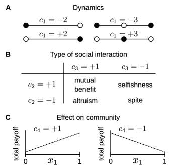
Figure S5: Case differentiation of game characteristics. An evolutionary game with two strategies and constant payoff has one out of (A) four possible dynamical structures (either two or three stationary states with the first one either stable or unstable), (B) four possible combinations of strategy 1’s impact on the payoff of the individuals (positive or negative impact on the payoff of strategy 1 and 2 players), and (C) two possible kinds of strategy 1’s impact on the total payoff of all players (positive or negative).

Name	Payoff rank criteria	Generalized criteria
Hawk-Dove	$[3,2,4,1]$ $[1,4,2,3]$	$[+3,+1,+1,+1]$ $[+3,-1,-1,-1]$
Battle	$[2,3,4,1]$ $[1,4,3,2]$	$[+3,-1,+1,+1]$ $[+3,-1,+1,-1]$
Hero	$[1,3,4,2]$ $[2,4,3,1]$
Compromise	$[1,2,4,3]$ $[3,4,2,1]$	$[-2,-1,+1,-1]$ $[+2,-1,+1,+1]$
Deadlock	$[2,1,4,3]$ $[3,4,1,2]$	$[-2,+1,+1,-1]$ $[+2,-1,-1,+1]$
Prisoner’s Dilemma	$[3,1,4,2]$ $[2,4,1,3]$	$[-2,+1,+1,+1]$ $[+2,-1,-1,-1]$
Stag Hunt	$[4,1,3,2]$ $[2,3,1,4]$	$[-3,+1,+1,+1]$ $[-3,-1,-1,-1]$
Assurance	$[4,1,2,3]$ $[3,2,1,4]$	$[-3,+1,-1,+1]$ $[-3,+1,-1,-1]$
Coordination	$[4,2,1,3]$ $[3,1,2,4]$
Peace	$[4,3,1,2]$ $[2,1,3,4]$	$[+2,+1,-1,+1]$ $[-2,+1,-1,-1]$
Harmony	$[4,3,2,1]$ $[1,2,3,4]$	$[+2,+1,+1,+1]$ $[-2,-1,-1,-1]$
Concord	$[4,2,3,1]$ $[1,3,2,4]$

Table S1: Criteria for strict symmetric games. The middle column shows the rank of the values in the payoff matrix $M=[a,b,c,d]$, e. g. $[3,2,4,1]$ means $d<b<a<c$ Bruns2015 . The right column shows the values of the criteria defined in the text.

References

- (1) A. Traulsen and M.A. Nowak. Evolution of cooperation by multilevel selection. Proc Natl Acad Sci U S A, 103(29):10952–10955, 2006.
- (2) L. Lehmann, L. Keller, S. West and D. Roze. Group selection and kin selection: Two concepts but one process. Proc Natl Acad Sci U S A, 104(16):6736–6739, 2007.
- (3) M.A. Nowak. Five rules for the evolution of cooperation. Science, 314(5805):1560–1563, 2006.
- (4) M.A. Nowak and R.M. May. Evolutionary games and spatial chaos. Nature, 359(6398):826–829, 1992.
- (5) C. Van den Broeck, J.M.R. Parrondo, R. Toral and R. Kawai. Nonequilibrium phase transitions induced by multiplicative noise. Phys Rev E, 55(4):4084–4094, 1997.
- (6) R. Toral. Noise-induced transitions vs. noise-induced phase transitions. AIP Conf Proc, 1332:145-154, 2011.
- (7) W. Horsthemke and R. Lefever. Noise-Induced Transitions: Theory and Applications in Physics, Chemistry, and Biology. Springer, 1984.
- (8) L. Gammaitoni, P. Hänggi, P. Jung and F. Marchesoni. Stochastic resonance. Rev Mod Phys, 70(1):223–287, 1998.
- (9) A. Lipshtat, A. Loinger, N.Q. Balaban and O. Biham. Genetic Toggle Switch without Cooperative Binding. Phys Rev Lett, 96:188101, 2006.
- (10) T. Biancalani and M. Assaf. Genetic Toggle Switch in the Absence of Cooperative Binding: Exact Results. Phys Rev Lett, 115:208101, 2015.
- (11) E.G. Leigh. The average lifetime of a population in a varying environment. J Theor Biol, 90(2):213–239, 1981.
- (12) R. Lande. Risks of population extinction from demographic and environmental stochasticity and random catastrophes. Am Nat, 142(6):911–927, 1993.
- (13) P. Foley. Predicting extinction times from environmental stochasticity and carrying capacity. Conserv Biol, 8(1):124–137, 1994.
- (14) O. Ovaskainen and B. Meerson. Stochastic models of population extinction. Trends Ecol Evol, 25(11):643–652, 2010.
- (15) S.J. Schreiber. Interactive effects of temporal correlations, spatial heterogeneity and dispersal on population persistence. Proc Biol Sci, 277(1689):1907–1914, 2010.
- (16) L.M. Morales. Viability in a pink environment: why “white noise” models can be dangerous. Ecol Lett, 2(4):228–232, 1999.
- (17) M. Heino, J. Ripa, and V. Kaitala. Extinction risk under coloured environmental noise. Ecography, 23(2):177–184, 2000.
- (18) C.C. Wilmers, E. Post, and A. Hastings. A perfect storm: The combined effects on population fluctuations of autocorrelated environmental noise, age structure, and density dependence. Am Nat, 169(5):673–683, 2007.
- (19) M. Schwager, K. Johst, and F. Jeltsch. Does red noise increase or decrease extinction risk? Single extreme events versus series of unfavorable conditions. Am Nat, 167(6):879–888, 2006.
- (20) M. Heino and M. Sabadell. Influence of coloured noise on the extinction risk in structured population models. Biol Conserv, 110(3):315–325, 2003.
- (21) L. Ruokolainen, A. Lindén, V. Kaitala, and M.S. Fowler. Ecological and evolutionary dynamics under coloured environmental variation. Trends Ecol Evol, 24(10):555–563, 2009.
- (22) J.V. Greenman and T.G. Benton. The impact of environmental fluctuations on structured discrete time population models: Resonance, synchrony and threshold behaviour. Theor Popul Biol, 68(4):217–235, 2005.
- (23) A. Kamenev, B. Meerson, and B. Shklovskii. How colored environmental noise affects population extinction. Phys Rev Lett, 101:268103, 2008.
- (24) M.A. Nowak, A. Sasaki, C. Taylor, and D. Fudenberg. Emergence of cooperation and evolutionary stability in finite populations. Nature, 428(6983):646–650, 2004.
- (25) A. Traulsen, M.A. Nowak, and J.M. Pacheco. Stochastic dynamics of invasion and fixation. Phys Rev E, 74(1):011909, 2006.
- (26) P.M. Altrock and A. Traulsen. Fixation times in evolutionary games under weak selection. New J Phys, 11:013012, 2009.
- (27) M. Assaf, M. Mobilia, and E. Roberts. Cooperation dilemma in finite populations under fluctuating environments. Phys Rev Lett, 111(23):238101, 2013.
- (28) P. Ashcroft, P.M. Altrock, and T. Galla. Fixation in finite populations evolving in fluctuating environments. J R Soc Interface, 11(100), 2014.
- (29) B. Houchmandzadeh. Fluctuation driven fixation of cooperative behavior. Biosystems, 127(0):60–66, 2015.
- (30) J.W. Baron and T. Galla. Sojourn times and fixation dynamics in multi-player games with fluctuating environments. arXiv, 1612.05530 [q-bio.PE], 2016.
- (31) D. Foster and P. Young. Stochastic evolutionary game dynamics. Theor Popul Biol, 38(2):219–232, 1990.
- (32) D. Fudenberg and C. Harris. Evolutionary dynamics with aggregate shocks. J Econ Theory, 57(2):420–441, 1992.
- (33) J. Hofbauer and L.A. Imhof. Time averages, recurrence and transience in the stochastic replicator dynamics. Ann Appl Probab, 19(4):1347–1368, 2009.
- (34) A. Traulsen, T. Röhl, and H.G. Schuster. Stochastic gain in population dynamics. Phys Rev Lett, 93(2):028701, 2004.
- (35) B. Houchmandzadeh and M. Vallade. Selection for altruism through random drift in variable size populations. BMC Evol Biol, 12(61), 2012.
- (36) W. Huang, C. Hauert, and A. Traulsen. Stochastic game dynamics under demographic fluctuations. Proc Natl Acad Sci U S A, 112(29):9064–9069, 2015.
- (37) C.S. Gokhale and C. Hauert. Eco-evolutionary dynamics of social dilemmas. Theor Popul Biol, 111:28–42, 2016.
- (38) G.W.A. Constable, T. Rogers, A.J. McKane, and C.E. Tarnita. Demographic noise can reverse the direction of deterministic selection. Proc Natl Acad Sci U S A, 113(32), 2016.
- (39) C. Taylor, D. Fudenberg, A. Sasaki, and M.A. Nowak. Evolutionary game dynamics in finite populations. Bull Math Biol, 66(6):1621–1644, 2004.
- (40) P. A. P. Moran. Random processes in genetics. Math Proc Cambridge Philos Soc, 54(1):60–71, 1958.
- (41) R.C. Lewontin and D. Cohen. On population growth in a randomly varying environment. Proc Natl Acad Sci U S A, 62(4):1056–1060, 1969.
- (42) O. Peters. Optimal leverage from non-ergodicity. Quant Finance, 11(11):1593–1602, 2011.
- (43) O. Peters and W. Klein. Ergodicity breaking in geometric brownian motion. Phys Rev Lett, 110(100603), 2013.
- (44) J.M. Smith. Evolution and the Theory of Games. Cambridge university press, 1982.
- (45) P.D. Taylor and L.B. Jonker. Evolutionary stable strategies and game dynamics. Math Biosci, 40(1-2):145–156, 1978.
- (46) J. Gore, H. Youk, and A. van Oudenaarden. Snowdrift game dynamics and facultative cheating in yeast. Nature, 459:253–256, 2009.
- (47) M Pigliucci. Evolution of phenotypic plasticity: where are we going now? Trends Ecol Evol, 20(9):481–486, 2005.
- (48) T.C. Bergstrom. On the evolution of hoarding, risk-taking, and wealth distribution in nonhuman and human populations. Proc Natl Acad Sci U S A, 111:10860–10867, 2014.
- (49) P.E. Turner and L. Chao. Escape from prisoner’s dilemma in RNA phage 6. Am Nat, 161(3):497–505, 2003.
- (50) E.A. Yurtsev, H.X. Chao, M.S. Datta, T. Artemova, and J. Gore. Bacterial cheating drives the population dynamics of cooperative antibiotic resistance plasmids. Mol Syst Biol, 9(683), 2013.
- (51) B.C. Kirkup and M.A. Riley. Antibiotic-mediated antagonism leads to a bacterial game of rock-paper-scissors in vivo. Nature, 428(6981):412–414, 2004.
- (52) A.S. Griffin, S.A. West, and A. Buckling. Cooperation and competition in pathogenic bacteria. Nature, 430(7003):1024–1027, 2004.
- (53) L.A. Dugatkin, M. Perlin, J. Scott Lucas, and R. Atlas. Group-beneficial traits, frequency-dependent selection and genotypic diversity: an antibiotic resistance paradigm. Proc R Soc London Ser B, 272(1558):79–83, 2005.
- (54) M.G.J. de Vos, M. Zagorski, A. McNally and T. Bollenbach. Interaction networks, ecological stability, and collective antibiotic tolerance in polymicrobial infections. PNAS, 114(40):10666–10671, 2017.
- (55) J. Stachurski and V. Martin. Computing the distributions of economic models via simulation. Econometrica, 76(2):443–450, 2008.
- (56) A. Traulsen, J.C. Claussen, and C. Hauert. Coevolutionary dynamics in large, but finite populations. Phys Rev E, 74(011901), 2006.
- (57) B. Bruns. Names for games: Locating 2 x 2 games. Games, 6(4):495–520, 2015.

References

- (1) J. Stachurski and V. Martin. Computing the distributions of economic models via simulation. Econometrica, 76(2):443–450, 2008.
- (2) A. Traulsen, J.C. Claussen, and C. Hauert. Coevolutionary dynamics in large, but finite populations. Phys Rev E, 74(011901), 2006.
- (3) B. Bruns. Names for games: Locating 2 x 2 games. Games, 6(4):495–520, 2015.