Practical Bayesian Modeling and Inference for Massive Spatial Datasets On Modest Computing Environments

Abstract

[Summary]With continued advances in Geographic Information Systems and related computational technologies, statisticians are often required to analyze very large spatial datasets. This has generated substantial interest over the last decade, already too vast to be summarized here, in scalable methodologies for analyzing large spatial datasets. Scalable spatial process models have been found especially attractive due to their richness and flexibility and, particularly so in the Bayesian paradigm, due to their presence in hierarchical model settings. However, the vast majority of research articles present in this domain have been geared toward innovative theory or more complex model development. Very limited attention has been accorded to approaches for easily implementable scalable hierarchical models for the practicing scientist or spatial analyst. This article devises massively scalable Bayesian approaches that can rapidly deliver inference on spatial process that are practically indistinguishable from inference obtained using more expensive alternatives. A key emphasis is on implementation within very standard (modest) computing environments (e.g., a standard desktop or laptop) using easily available statistical software packages. Key insights are offered regarding assumptions and approximations concerning practical efficiency.

1 Introduction

Rapidly increasing usage and growing capabilities of Geographic Information Systems (GIS) have spawned considerable research in modeling and analyzing spatial datasets in diverse disciplines including, but not limited to, environmental sciences, economics, biometry and so on see, e.g., ¹⁴, ⁸, ³. Much of spatial modeling is carried out within the familiar hierarchical modeling paradigm,

$$[\mbox{data}\,|\,\mbox{process}]\times[\mbox{process}\,|\,\mbox{parameters}]\times[\mbox{parameters}]\;.$$ (1)

For point-referenced data sets, where spatial locations are indexed by coordinates on a map, the “process” is modeled as a spatial random field over the domain of interest and the observations are treated as a finite realization of this random field. The Gaussian process (GP) is, perhaps, the most conspicuous of process specifications and offers flexibility and richness in modeling. The GP’s popularity as a modeling tool is enhanced due to their extensibility to multivariate and spatial-temporal geostatistical settings, although we do not pursue such generalizations in this article. They also provide comparatively greater theoretical tractability among spatial processes ³³.

Fitting GPs incur onerous computational costs that severely hinders their implementation for large datasets. The key bottleneck stems from the massive spatial covariance matrix present in the multivariate normal density for the finite realizations of the GP. For irregularly situated spatial locations, as is common in geostatistics, these matrices are typically dense and carry no exploitable structure to facilitate computations. Even for a modestly large number of points ($\approx 50,000$ or greater), the computational demands become prohibitive for a modern computer and preclude inference from GP models.

A substantial literature exists on methodologies for massive spatial datasets and it is already too vast to be summarized here see, e.g., ², ¹⁹ and references therein. Some are more amenable than others to the hierarchical setup in (1). Even within the hierarchical paradigm, there is already a burgeoning literature on massively scalable spatial process models. There are two pressing issues facing the practicing spatial analyst. The first is to analyze massive amounts of spatial data on “modest” computing environments such as standard desktop or laptop architectures. The second pressing issue is that of full inference that subsumes parameter estimation, spatial prediction of the outcome, and estimation of the underlying latent process. Yet the size of the datasets easily exceed the CPU memory available for computing, which means that we need to rely upon statistical models that will enable analysis with the available memory.

Some scalable processes such as the multi-resolution predictive process models proposed by ²¹ or the nearest-neighbor Gaussian process (NNGP) models by ⁹ can be programmed in modest computing environments to estimate parameters and predict outcomes, but not necessarily infer on the latent process efficiently. ²¹ does not address this, while ⁹ and ¹⁰ implement high-dimensional Gibbs sampling algorithms that had to be run for several iterations on a high-performance computing environment to yield adequate convergence due to high autocorrelations. Other approaches such as Gaussian Markov random field (GMRF) approximations to spatial processes ^{30, 24} use Integrated Nested Laplace Approximations (INLA) for computing the marginal distribution of the process at given locations. These approximations can be implemented on standard environments for a variety of spatial models using the R-INLA software (www.r-inla.org). This is computationally more promising than MCMC, but is still an iterative procedure requiring convergence assessment. Its performance is yet to be demonstrated for analyzing massive spatial data with millions of spatial locations on modest computing environments.

This article outlines strategies for achieving fully model-based Bayesian inference including parameter estimation, response surface predictions and interpolation of the latent spatial process for massive spatial datasets on modest computing environments. To achieve this goal, we need a massively scalable spatial process that will be able to estimate (1) by obviating the memory obstacles. Here, there are a few choices that are well-suited for (1) all of whom seem to be competitive based upon the recent “contest” paper by ¹⁹, but we opt for the sparsity-inducing Nearest-neighbor Gaussian process (NNGP) primarily because of its ease of use and also because of its easier accessibility through the spNNGP package available from cran.r-project.org/web/packages/spNNGP (see Section 2).

In fact, Finley et al. ¹² outlines several strategies for estimating NNGP models, including a conjugate response NNGP model and a collapsed NNGP model. The conjugate response NNGP model can provide exact inference without requiring MCMC and has been demonstrated to effectively fit a dataset with approximately 5 million locations in a matter of seconds on a Linux workstation. However, the response model does not accommodate the latent process and, hence, is restrictive in its inferential capabilities compared to (1). The collapsed NNGP model, on the other hand, is embedded within MCMC algorithms and is able to provide the posterior inference of the latent process. It can exploit permutation-based sparse Cholesky methods, but the approach requires specialized libraries and can still be too expensive for massive datasets in the order of $10^{6}$ locations for standard computing environments. We briefly introduce the conjugate response NNGP model in section 3.2, and the discussion of the collapsed NNGP model can be found in section 2.2. Our contribution lies in casting the latent process models of ⁹ within a conjugate Bayesian framework for exact inference so as to avoid MCMC while being able to achieve full Bayesian inference including estimation of the latent process. We propose a conjugate latent NNGP model that exploits conjugacy in conjunction with cross-validatory estimation of a small set of process parameters, and the model formulation and computations will not require loading large data objects into memory at any point, allowing fitting for massive datasets in the order of $10^{6}$ on computer environments like standard desktop or laptop architecture. The details of this Bayesian formulation and the algorithms for their effective implementation constitute the novelty of this paper.

The remainder of the paper evolves as follows. Section 2 provides a brief review of nearest-neighbor Gaussian process and NNGP based models. Section 3 develops the conjugate NNGP based models, emphasizing the conjugate latent NNGP model, and devises algorithms for practical implementation. A simulation study is presented in Section 4 for discussing the performance of the proposed models, while an analysis on sea surface temperature with over 2.5 million locations is conducted in Section 5. Finally, we conclude with some discussion in Section 6.

2 The nearest-neighbor Gaussian process

The computational burden in GP models arises from the $n\times n$ covariance matrix $C_{\theta}(S,S)$, where $S=\{s_{1},s_{2},\ldots,s_{n}\}$ is the set of observed locations. The $(i,j)$-th element of this matrix is the value of a spatial covariance function evaluated at locations $s_{i}$ and $s_{j}$. Spatial covariance functions in general do not produce exploitable structures in the resulting matrices. One effective approach to achieve efficient computations is to replace $C_{\theta}(S,S)$ with an approximate $\tilde{C}_{\theta}(S,S)$ such that the inverse of $\tilde{C}_{\theta}(S,S)$ is sparse. There are multiple options, but notable among them are approximations based upon Gaussian Markov random fields or GMRFs see, e.g., ²⁹, ³⁰ that yield computationally efficient sparse representations. An alternative approach exploits an idea familiar in graphical models or Bayesian networks see, e.g., ²³, ⁶, ²⁵ that has also been exploited by ³⁶, ³⁴ and ³⁵ to construct composite likelihoods for inference. Datta et al. ⁹, Datta et al. ¹⁰ extended this idea to construct a Nearest Neighbor Gaussian Process (NNGP) for modeling large spatial data. NNGP is a well defined Gaussian Process that yields finite dimensional Gaussian densities with sparse precision matrices. It delivers massive scalability both in terms of parameter estimation and spatial prediction or “kriging”.

2.1 Response NNGP model

Consider modeling a point-referenced outcome as a partial realization of a Gaussian process, $\{y(s):s\in D\}\sim GP(m_{\theta}(s),C_{\theta}(\cdot,\cdot))$ on a spatial domain $D\in\Re^{d}$. The mean and covariance functions are assumed to be determined by one or more parameters in a set $\theta$. The finite-dimensional distribution for the $n\times 1$ vector $y(S)$ with elements $y(s_{i})$ is multivariate normal with mean $m_{\theta}(S)$ and covariance matrix $C_{\theta}(S,S)$. As a directed acyclic graph (DAG) ⁶, the joint density is $\displaystyle p(y(S))=\prod_{i=1}^{n}p(y(s_{i})\,|\,y(\mbox{Pa}[s_{i}])$, where $\mbox{Pa}[s_{1}]$ is the empty set and $\mbox{Pa}[s_{i}]=\{s_{1},s_{2},\ldots,s_{i-1}\}$ for $i=2,3,\ldots,n-1$ is the set of parent nodes with directed edges to $s_{i}$. ³⁶ suggested approximating the multivariate normal likelihood by shrinking $\mbox{Pa}[s_{i}]$ from the set of all nodes preceding $s_{i}$ to a much smaller subset of locations preceding $s_{i}$ that are among the $m$ (a fixed small number) nearest neighbors of $s_{i}$ based upon their Euclidean distance. ⁹ extended that notion to arbitrary points in the domain by defining

$$\mbox{Pa}[s]=\left\{\begin{array}[]{ll}\mbox{empty set}&\mbox{ if $s=s_{1}$}\;,\\ \{s_{1},s_{2},\ldots,s_{i-1}\}&\mbox{ if $s\in S$ and $i=1,2,\ldots,m$}\;,\\ \mbox{$m$ closest points to $s$ among $\{s_{1},s_{2},\ldots,s_{i-1}\}$}&\mbox{ if $s\in S$ and $i>m$}\;,\\ \mbox{$m$ closest points to $s$ among $S$}&\mbox{ if $s\notin S$}\;.\end{array}\right.$$

for any arbitrary point $s$ in the domain, where $m$ is the fixed number of nearest neighbors. This results in another multivariate Gaussian density

$$p(y(S)) =N(y(S)\,|\,m_{\theta}(S),C_{\theta}(S,S))\approx N(y(S)\,|\,m_{\theta}(S),\tilde{C}_{\theta}(S,S))\;,$$ (2)

where $\tilde{C}_{\theta}(S,S)^{-1}=(I-A_{S})^{\top}D_{S}^{-1}(I-A_{S})$ is sparse, $A_{S}$ is sparse and strictly lower triangular with $A_{S}(i,i)=0$ for $i=1,2,\ldots,n$ and at most $m$ non-zero entries in each row, and $D_{S}$ is diagonal whose elements are the conditional variances $\mbox{var}\{y(s_{i})\,|\,y(\mbox{Pa}[s_{i}])\}$ based upon the full GP model, i.e., $D_{S}(1,1)=C_{\theta}(s_{1},s_{1})$ and $D_{S}(i,i)=C_{\theta}(s_{i},s_{i})-C_{\theta}(s_{i},\mbox{Pa}[s_{i}])C_{\theta}(\mbox{Pa}[s_{i}],\mbox{Pa}[s_{i}])^{-1}C_{\theta}(\mbox{Pa}[s_{i}],s_{i})$ for $i=2,\ldots,n$. Turning to the structure of $A_{S}$, all its elements are completely determined from $C_{\theta}(S,S)$. Its first row, i.e., $A_{S}(1,)$ has all zeroes. For the $i+1$-th row, the nonzero entries appear in the positions indexed by $\mbox{Pa}[s_{i+1}]$ and are obtained as row vectors,

$$A_{S}(i+1,\mbox{Pa}[s_{i+1}])=C_{\theta}(s_{i+1},\mbox{Pa}[s_{i+1}])C_{\theta}(\mbox{Pa}[s_{i+1}],\mbox{Pa}[s_{i+1}])^{-1}\;.$$

The nonzero entries in each row of $A_{S}$ are precisely the “kriging” weights of $y(s_{i})$ based upon the values of $y(s)$ at neighboring locations, i.e., $\mbox{Pa}[s_{i}]$ ⁷. The $\tilde{C}_{\theta}(S,S)$, constructed as above, is called an NNGP approximation to $C_{\theta}(S,S)$.

With the above definition of $\mbox{Pa}[s]$, we can express the partial realizations of an NNGP as a linear model. Let $S$ be the set of the $n$ observed locations as defined earlier (and $n$ is assumed to be large) and let $U=\{u_{1},u_{2},\ldots,u_{n^{\prime}}\}$ be a set of $n^{\prime}$ arbitrary locations where we wish to predict $y(s)$. Then,

$$\underbrace{\left[\begin{array}[]{c}y(S)\\ y(U)\end{array}\right]}_{y}=\underbrace{\left[\begin{array}[]{c}m_{\theta}(S)\\ m_{\theta}(U)\end{array}\right]}_{m_{\theta}}+\underbrace{\left[\begin{array}[]{c}A(S)\\ A(U)\end{array}\right]}_{A}(y(S)-m_{\theta}(S))+\underbrace{\left[\begin{array}[]{c}\eta(S)\\ \eta(U)\end{array}\right]}_{\eta}\;,$$ (3)

where $\displaystyle\eta\sim N\left(\left[\begin{array}[]{c}0\\ 0\end{array}\right],\left[\begin{array}[]{cc}D(S)&O\\ O&D(U)\end{array}\right]\right)$, $D(U)$ is $n^{\prime}\times n^{\prime}$ diagonal and $A(U)$ is sparse $n^{\prime}\times n$ formed by extending the definitions of $D(S)$ and $A(S)$ as

$$D(U)(i,i) =C_{\theta}(u_{i},u_{i})-C_{\theta}(u_{i},\mbox{Pa}[u_{i}])C_{\theta}(\mbox{Pa}[u_{i}],\mbox{Pa}[u_{i}])^{-1}C_{\theta}(\mbox{Pa}[u_{i}],u_{i})\;,$$ (4)

$$A(U)(i,\mbox{Pa}[u_{i}]) =C_{\theta}(u_{i},\mbox{Pa}[u_{i}])C_{\theta}(\mbox{Pa}[u_{i}],\mbox{Pa}[u_{i}])^{-1}\;.$$

Each row of $A(U)$ has exactly $m$ nonzero entries corresponding to the column indices in $\mbox{Pa}[u_{i}]$. The above structure implies that $y(s)$ and $y(s^{\prime})$ are conditionally independent for any two points $s$ and $s^{\prime}$ outside of $S$, given $y(S)$. The parameters $\theta$ will be estimated from the data $y(S)$ and predictions will be carried out using the conditional distribution of $y(U)$ given $y(S)$. In a Bayesian setting, $\theta$ will be sampled from its posterior distribution $p(\theta\,|\,y(S))$,

$$p(\theta)\times\left(\prod_{i=1}^{n}\frac{1}{\sqrt{D(S)(i,i)}}\right)\times\exp\left\{-\frac{1}{2}z_{\theta}(S)^{\top}(I-A(S)^{\top})D(S)^{-1}(I-A(S))z_{\theta}(S)\right\}\;,$$ (5)

where $z_{\theta}(S)=y(S)-m_{\theta}(S)$ and $p(\theta)$ is the prior distribution for $\theta$.

Consider a specific example with the covariance function $C_{\theta}(s,s^{\prime})=\sigma^{2}\exp(-\phi\|s-s^{\prime}\|)+\tau^{2}\delta_{s=s^{\prime}}$, where $\delta_{s=s^{\prime}}$ is equal to one if $s=s^{\prime}$ and $0$ otherwise, and $m_{\theta}=x(s)^{\top}\beta$ is a linear regression with spatial predictors $x(s)$ and corresponding slope vector $\beta$. Then $\theta=\{\beta,\sigma^{2},\phi,\tau^{2}\}$ and one choice of priors could be

$$p(\theta)\propto U(\phi\,|\,a_{\phi},b_{\phi})\times IG(\sigma^{2}\,|\,a_{\sigma},b_{\sigma})\times IG(\tau^{2}\,|\,a_{\tau},b_{\tau})\times N(\beta\,|\,\mu_{\beta},V_{\beta})\;,$$

where we are using standard notations for the above distributions as, e.g., in Gelman et al. ¹⁵. The parameter space for this model is not high-dimensional and MCMC algorithms such as Gibbs sampling in conjunction with random-walk Metropolis (RWM) or Hamiltonian Monte Carlo (HMC) can be easily implemented. Other approximate algorithms such as Variational Bayes or INLA can also be used.

Once the parameter estimates (i.e., posterior samples) are obtained from (5) we can carry out predictive inference for $y(U)$ from the posterior predictive distribution

$$p(y(U)\,|\,y(S)) =\int p(y(U)\,|\,y(S),\theta)p(\theta\,|\,y(S))d\theta=\mbox{E}_{\theta\,|\,y(S)}\left[N(y(U)\,|\,\mu_{\theta}(U|\cdot),D(U))\right]\;,$$ (6)

where $p(y(U)\,|\,y(S),\theta)$ is an $n^{\prime}$-dimensional multivariate normal distribution with mean $\mu_{\theta}(U|\cdot)=m_{\theta}(U)+A(U)(y(S)-m_{\theta}(S))$ and conditional covariance matrix $D(U)$. Since $D(U)$ is diagonal, it is easy to sample from $p(y(U)\,|\,y(S),\theta)$. For each $\theta$ sampled from (5), we sample an $n^{\prime}$-dimensional vector $y(U)$ from $p(y(U)\,|\,y(S),\theta)$. The resulting $y(U)$’s are samples from (6). The NNGP exploits the conditional independence between the elements of $y(U)$, given $y(S)$ and $\theta$, to achieve efficient posterior predictive sampling for $y(U)$. This assumption of conditional independence is not restrictive as the samples from (6) are not independent. In fact, the marginal covariance matrix of $y(U)$, given $\theta$ only, is $A(U)\tilde{C}_{\theta}(S,S)A(U)^{\top}+D(U)$, which is clearly not diagonal.

2.2 Latent NNGP model

Rather than model the outcome as an NNGP, as was done for the response model in the preceding subsection, one could use the NNGP as a prior for the latent process ⁹. In fact, as discussed in Section 4 of ⁹, the response model does not strictly follow the paradigm in (1) and it is not necessarily possible to carry out inference on a latent or residual spatial process after accounting for the mean.

A more general setting envisions a spatial regression model at any location $s$

$$y(s)=m_{\theta}(s)+w(s)+\epsilon(s)\;,\quad\epsilon(s)\stackrel{{\scriptstyle iid}}{{\sim}}N(0,\tau^{2})\;,$$ (7)

where, usually, $m_{\theta}(s)=x(s)^{\top}\beta$ and $w(s)$ is a latent spatial process capturing spatial dependence. Using definitions analogous to Section 2.1, we assume $\{w(s):s\in D\}\sim NNGP(0,\tilde{C}_{\theta}(\cdot,\cdot))$, which means that for any $S$ and $U$, as constructed in (3), $w\equiv w(S\cup U)$ will have a zero-centered multivariate normal law with covariance matrix $(I-A)^{-1}D(I-A)^{-\top}$. The posterior distribution to be sampled from is now given by

$$p(\theta)\times N(w\,| 0,\tilde{C}_{\theta}(S,S))\times\prod_{i=1}^{n}N(y(s_{i})\,|\,m_{\theta}(s_{i})+w(s_{i}),\tau^{2})\;.$$ (8)

It is easier to sample from (5) than from (8) since the parameter space in the latter includes the high-dimensional random vector $w$ in addition to $\theta$. One option is to integrate out $w$ from (8) which yields the posterior

$$p(\theta)\times(\mbox{det}(\tilde{C}_{\theta}(S,S)+\tau^{2}I_{n}))^{-\frac{1}{2}}\times\exp\left\{-\frac{1}{2}\sum_{i=1}^{n}z_{\theta}(S)^{\top}\left(\tilde{C}_{\theta}(S,S)+\tau^{2}I_{n}\right)^{-1}z_{\theta}(S)\right\}\;,$$ (9)

where $\mbox{det}(A)$ is the determinant of matrix $A$, $p(\theta)$ and $z_{\theta}(S)$ are as defined for (5). The parameter space has collapsed from $\{\theta,w\}$ to $\theta$, so (9) is called the collapsed version of (8). Efficient computations for obtaining (9) requires a sparse-Cholesky decomposition for the large matrix $\left(\tilde{C}_{\theta}(S,S)^{-1}+\tau^{-2}I\right)$. This step can be complicated and expensive. To exacerbate the matter further, full Bayesian inference requires calculating the likelihood (9) in each MCMC iteration as described in the algorithm of the “collapsed” model in Section 2.1 of Finley et al. ¹². To avoid such expenses, we turn to conjugate models in the next section.

3 Conjugate Bayesian model

The response NNGP and latent NNGP models outlined in Sections 2.1 and 2.2, respectively, will still require iterative simulation methods such as MCMC for full Bayesian inference. Conjugate models, i.e., using conjugate priors, can provide exact Bayesian inference by exploiting analytic forms for the posterior distributions. While some specific assumptions are needed, these models are much faster to implement even for massive datasets. Here we develop conjugate NNGP models using the tractable Normal Inverse-Gamma (NIG) family of conjugate priors. We formulate a conjugate response model (also formulated in ¹² and is available in the spNNGP package from cran.r-project.org/web/packages/spNNGP) and a new conjugate latent NNGP model. These are conjugate versions of the models described in Sections 2.1 and 2.2. We especially focus on the conjugate latent NNGP model and show how it can exploit sparsity by sampling from latent spatial processes over massive numbers of locations efficiently using a conjugate gradient algorithm for solving large sparse systems.

3.1 The NIG conjugate prior family

Let the spatial linear regression model be specified as

$$y(S)=X\beta+w(S)+\epsilon(S)$$ (10)

where $y(S)$, $w(S)$ and $\epsilon(S)$ are the realization of the corresponding processes defined in (7) over the $n$ observed locations $S=\{s_{1},\ldots,s_{n}\}$, $X$ is the $n\times p$ matrix of regressors with $i$-th row being a $1\times p$ vector of regressors, $x(s_{i})^{\top}$ at location $s_{i}\in S$. Henceforth, we suppress the dependence of $y$, $w$, $\epsilon$ and their covariance matrix on $S$ when this will not lead to confusion. Assume that $w\sim N(0,\sigma^{2}C)$, $\epsilon\sim N(0,\delta^{2}\sigma^{2}I_{n})$, where $C$ and $\delta^{2}=\frac{\tau^{2}}{\sigma^{2}}$ are known. Let $\gamma^{\top}=[\beta^{\top},w^{\top}]$, $\mu_{\gamma}^{\top}=[\mu_{\beta}^{\top},O^{\top}]$ and $V_{\gamma}=\left[\begin{array}[]{cc}V_{\beta}&O\\ O&C\end{array}\right]$. The Normal-Inverse-Gamma (NIG) density yields a convenient conjugate prior,

$$p(\gamma,\sigma^{2}) =NIG(\gamma,\sigma^{2}\,|\,\mu_{\gamma},V_{\gamma},a,b)=N(\gamma\,|\,\mu_{\gamma},\sigma^{2}V_{\gamma})\times IG(\sigma^{2}\,|\,a,b)\;.$$ (11)

The posterior distribution of the parameters, up to proportionality, is

$$p(\gamma,\sigma^{2}\,|\,y)\propto NIG(\gamma, \sigma^{2}\,|\,\mu_{\gamma},V_{\gamma},a_{\sigma},b_{\sigma})\times N(y\,|\,[X:I_{n}]\gamma,\delta^{2}\sigma^{2}I_{n})\;.$$ (12)

The joint posterior distribution is of the form $NIG(\mu^{*},V^{*},a^{*},b^{*})$, where

$$\begin{array}[]{ll}y^{*}&={1\over\delta}y\;,\quad X^{*}=\left[{1\over\delta}X,{1\over\delta}I_{n}\right]\;,\\ \mu^{*}&=[V_{\gamma}^{-1}+X^{*\top}X^{*}]^{-1}(V_{\gamma}^{-1}\mu_{\gamma}+X^{*\top}y^{*})\;,\\ V^{*}&=[V_{\gamma}^{-1}+X^{*\top}X^{*}]^{-1}\;,\\ a^{*}&=a_{\sigma}+{n\over 2}\;,\\ b^{*}&=b_{\sigma}+{1\over 2}[\mu_{\gamma}^{\top}V_{\gamma}\mu_{\gamma}+y^{*\top}y^{*}-\mu^{*\top}V^{*-1}\mu^{*}]\;.\end{array}$$ (13)

The prior of the regression coefficients $\beta$ is formulated as $N(\mu_{\beta},V_{\beta})$. The above model, however, also allows improper priors for $\beta$. When assigning improper priors for $\beta$, the precision matrix of the prior of $\gamma$ in (13) becomes $V_{\gamma}^{-1}=\left[\begin{array}[]{cc}O&O\\ O&C^{-1}\end{array}\right]$, showing that no information from $\beta$‘s prior contributes to the posterior distribution, and we can assume $\mu_{\gamma}^{\top}=[O^{\top},O^{\top}]$ in (13). The marginal posterior distribution of $\sigma^{2}$ follows an $IG(a^{*},b^{*})$ and the marginal posterior distribution of $\gamma$ can be identified as a multivariate t-distribution with mean $\mu^{*}$, variance $\frac{b^{*}}{a^{*}}V^{*}$ and degree of freedom $2a^{*}$(i.e. $\text{MVS-}t_{2a^{*}}(\mu^{*},\frac{b^{*}}{a^{*}}V^{*})$). Exact Bayesian inference is carried out by sampling directly from the joint posterior density: we sample $\sigma^{2}$ from $IG(a^{*},b^{*})$ and then, for each sampled $\sigma^{2}$, we draw $\gamma$ from its conditional posterior density $N(\mu^{\ast},\sigma^{2}V^{\ast})$. This yields posterior samples from (12). Furthermore, note that once the posterior samples of $\sigma^{2}$ are obtained, we can obtain samples from $p(\tau^{2}\,|\,y)$ by simply multiplying the sampled $\sigma^{2}$s with $\delta^{2}$. Thus, posterior samples are obtained without recourse to MCMC or other iterative algorithms.

3.2 Conjugate response NNGP model

Finley et al. ¹² formulated a conjugate NNGP model for the response model described in Section 2.1. This is formed by integrating out $w(S)$ from (10) and applying an NNGP approximation to the marginal covariance matrix of $y(S)$. The model can be cast as a conjugate Bayesian linear regression model

$$p(\beta,\sigma^{2}\,|\,y)\propto NIG(\beta,\sigma^{2}\,|\,\mu_{\beta},V_{\beta},a_{\sigma},b_{\sigma})\times N(y\,|\,X\beta,\sigma^{2}\tilde{K})\;,$$ (14)

where $\tilde{K}$ is the NNGP approximation of $K=C+\delta^{2}I$, $C$ and $\delta^{2}$ are as described in Section 3.1. Also, $\tilde{K}^{-1}=\sigma^{2}(I-A(S)^{\top})D(S)^{-1}(I-A(S))$ with $A(S)$ and $D(S)$ as described in Section 2.1. We will refer to (14) as the conjugate response NNGP model. Note that this model can estimate $\{\beta,\sigma^{2}\}$ and also impute the outcome at unknown locations, but does not permit inference on the latent process $w(\cdot)$. The reason why a conjugate response NNGP model cannot provide inference on the latent process is that the construction of the response NNGP will not guarantee the existence of a well-defined latent process. It is pointed out in Section 4 of ⁹ that the eigenvalue of $\tilde{K}$ may be less than $\delta^{2}$, consequently the covariance matrix of the posterior distribution of $w$ need not be positive definite for every proper $\delta^{2}$, $\mu_{\beta}$ and $V_{\beta}$. We address this shortcoming with a new conjugate latent NNGP model in the next section.

3.3 Conjugate latent NNGP model

The conjugate models in Section 3.1 works for any covariance matrix $C$. Here, we derive a conjugate latent NNGP model that will subsume inference on $w(\cdot)$. We rewrite the covariance matrix $\tilde{C}_{\theta}(S,S)$ in section 2.2 for $w(S)$ as $\sigma^{2}\tilde{M}_{\phi}$ with fixed parameter $\phi$. Note that $\tilde{M}_{\phi}$ is the NNGP approximation of the dense matrix $M$, where $C=\sigma^{2}M$. Specifically, $\tilde{M}_{\phi}^{-1}=(I-A_{M})^{\top}D_{M}^{-1}(I-A_{M})$, where $A_{M}$ and $D_{M}$ depend only on $\phi$. We recast the model as

$$\begin{array}[]{c}\underbrace{\left[\begin{array}[]{c}{1\over\delta}y\\ L_{\beta}^{-1}\mu_{\beta}\\ 0\end{array}\right]}=\underbrace{\left[\begin{array}[]{cc}{1\over\delta}X&{1\over\delta}I_{n}\\ L_{\beta}^{-1}&O\\ O&D_{M}^{-{1\over 2}}(I-A_{M})\end{array}\right]}\underbrace{\left[\begin{array}[]{c}\beta\\ w\end{array}\right]}+\underbrace{\left[\begin{array}[]{c}\eta_{1}\\ \eta_{2}\\ \eta_{3}\end{array}\right]}\\ \hskip 5.69046pty_{*}\hskip 14.22636pt=\hskip 39.83368ptX_{*}\hskip 51.21504pt\gamma\hskip 11.38092pt+\hskip 11.38092pt\eta\end{array}$$ (15)

where $L_{\beta}$ is the Cholesky decomposition of the $p\times p$ matrix $V_{\beta}$, and $\eta\sim N(0,\sigma^{2}I_{2n+p})$. The joint posterior distribution of $\gamma$ and $\sigma^{2}$ follows an NIG distribution

$$p(\gamma,\sigma^{2}\,|\,y)=NIG(\gamma,\sigma^{2}\,|\,\hat{\gamma},(X_{*}^{\top}X_{*})^{-1},a_{*},b_{*})$$ (16)

where $\displaystyle\hat{\gamma}=(X_{*}^{\top}X_{*})^{-1}X_{*}^{\top}y_{*}$, $\displaystyle a_{*}=a_{\sigma}+{n\over 2}$ and $\displaystyle b_{*}=b_{\sigma}+{1\over 2}(y_{*}-X_{*}\hat{\gamma})^{\top}(y_{*}-X_{*}\hat{\gamma})$. Evaluating the posterior mean of $\gamma$ involves solving $X_{*}^{\top}X_{*}\hat{\gamma}=X_{*}^{\top}y_{*}$, which requires $\mathcal{O}({1\over 3}(n+p)^{3})$ flops. However, when $p\ll n$, the structure of $X_{*}$ ensures low storage complexity. Also, $X_{*}^{\top}X_{*}=$

$$\left[\begin{array}[]{cc}{1\over\delta^{2}}X^{\top}X+L_{\beta}^{-\top}L_{\beta}^{-1}&{1\over\delta^{2}}X^{\top}\\ {1\over\delta^{2}}X&{1\over\delta^{2}}I_{n}+(I_{n}-A_{M})^{\top}D_{M}^{-1}(I_{n}-A_{M})\end{array}\right]$$ (17)

Since $(I_{n}-A_{M})$ has less than $n(m+1)$ nonzero elements and each of its row has at most $m+1$ nonzero elements, the storage of the $n\times n$ matrix $(I_{n}-A_{M})^{\top}D_{M}^{-1}(I_{n}-A_{M})$ is less than $n(m+1)^{2}$, and the computational complexity is less than $nm+n(m+1)^{2}$.

This sparsity in $X_{*}^{\top}X_{*}$ can be exploited by a conjugate gradient (CG) method see, e.g., ¹⁷. CG is an iterative method for solving $Ax=b$ when $A$ is a symmetric positive definite matrix. The underlying idea is to recognize that a solution of the linear system $Ax=b$ minimizes the quadratic function $\phi(x)=\frac{1}{2}x^{\top}Ax-x^{\top}b$. CG is an iterative procedure that generates a sequence of approximate solutions $\{x_{k}\}_{k=1,2,\ldots}$ that converges to $x=A^{-1}b$ in at most $n$ iterations. Briefly, the procedure starts with an initial value $x_{0}$ and setting $r_{0}=b-Ax_{0}$ and $q_{0}=r_{0}$. Then, at the $k+1$-th iteration we compute the following three quantities for each $k=0,1,2,\ldots$: (i) $x_{k+1}=x_{k}+\frac{\|r_{k}\|^{2}}{q_{k+1}^{\top}Aq_{k+1}}q_{k+1}$; (ii) $r_{k+1}=b-Ax_{k+1}$; and (iii) $q_{k+1}=r_{k+1}+\left(\frac{\|r_{k+1}\|}{\|r_{k}\|}\right)^{2}q_{k}\;$. The matrix $A$ is involved only in matrix-vector multiplications. Due to the sparsity of $A$, the computational cost per iteration is $\mathcal{O}(n)$ flops. The sparsity in $A$ also implies that CG is more memory efficient than direct methods such as the Cholesky decomposition. A sufficiently good approximation is often obtained in iterations much less than $n$ ⁴, hence the performance of the conjugate gradient algorithm will be competitive when $n$ is large. This enables posterior sampling of the latent process $w(S)$ in high-dimensional settings. The algorithm for sampling $\{\gamma,\sigma^{2}\}$ from (16) using the conjugate gradient method is given below.

 
Algorithm 1: Sample $\{\gamma,\sigma^{2}\}$ from conjugate latent NNGP model
 

1. Fixing $\phi$ and $\delta^{2}$, obtain $L_{\beta}^{-1}\mu_{\beta}$ and $L_{\beta}^{-1}$:

   • Compute a Cholesky decomposition of $V_{\beta}$ to get $L_{\beta}$ $\mathcal{O}(p^{3})$

   • Compute $L_{\beta}^{-1}$ and $L_{\beta}^{-1}\mu_{\beta}$ $\mathcal{O}(p^{2})$

2. Obtain the posterior mean for $\gamma$:

   • Construct $A_{M}$ and $D_{M}$ as described, for example, in Finley et al. ¹² $\mathcal{O}(nm^{3})$

   • Construct $X_{*}$ and $Y_{*}$ from (15) $\mathcal{O}(nm)$

   • Calculate $X_{*}^{\top}X_{*}$ and $X_{*}^{\top}y_{*}$ $\mathcal{O}(n(m+1)^{2})$

   • Use conjugate gradient to solve $X_{*}^{\top}X_{*}\hat{\gamma}=X_{*}^{\top}y_{*}$

3. Obtain posterior samples of $\sigma^{2}$

   • Calculate $a_{*}$ and $b_{*}$ as given below (16) $\mathcal{O}(n(m+4+p))$

   • Sample $\sigma^{2}$ from $IG(a_{*},b_{*})$

4. Obtain posterior samples of $\gamma$

   • Generate $u\sim N(0,\sigma^{2}I_{2n+p})$

   • Calculate $v$ by solving $X_{*}^{\top}X_{*}v=X_{*}^{\top}u$ using conjugate gradient

   • Obtain $\gamma=\hat{\gamma}+v$ $\mathcal{O}(n)$

 

It is readily seen that the $v$ in step 4 follows a Gaussian distribution with variance $\sigma^{2}(X_{*}^{\top}X_{*})^{-1}$. Note that Algorithm 1 implements the conjugate gradient method for an $n+p$-dimensional linear system in steps 2 and 4. Since $X_{*}$ and $y_{*}$ depend only on $\{\phi,\delta^{2}\}$, the linear equation in step 2 only need to be solved once for each choice of $\{\phi,\delta^{2}\}$.

The main contribution of the conjugate gradient method lies in obtaining the posterior estimator $\hat{\gamma}$ (step 2) and generating samples from a high dimensional Gaussian distribution (step 4). It is worth pointing out that the conjugate gradient method does not easily produce the determinant of a large matrix. Hence, a sparse Cholesky decomposition is still unavoidable for the collapsed NNGP model formulated in equation (9), where $\det\left(\tilde{C}_{\theta}(S,S)+\tau^{2}I\right)$ changes with the hyper-parameters $\theta$.

3.4 Posterior predictive inference for conjugate latent NNGP

We extend the predictive inference for the response NNGP model in Section 2.1 to the conjugate latent NNGP model. Assume $w(U)$ and $y(U)$ are the realization of the latent process and the response process over the $n^{\prime}$ locations $U=\{u_{1},\ldots,u_{n^{\prime}}\}$ where we wish to predict. let $C_{\theta}(\cdot,\cdot)$ be the covariance function for the latent process $w(s)$ in (7), $Pa[u_{i}]$ be the nearest neighbors of $i$th location in $U$ as defined in section 2.1. Define $A_{u}=A(U)$ and $D_{u}=\frac{1}{\sigma^{2}}D(U)$ where $A(U)$ and $D(U)$ are constructed by (4). Here, $\sigma^{2}$ refers to the variance of the latent process $w(s)$, and $A_{u}$ and $D_{u}$ are defined in the way that they only depend on fixed parameter $\phi$. According to the definition of NNGP process over the whole domain given in section 2, the joint distribution of $w(U)$ and $\gamma,\sigma^{2}$ given $y(S)$ follows:

$$p(w(U),\gamma,\sigma^{2}\,|\,y(S))=N(w(U)\,|\,[O:A_{u}]\gamma,\sigma^{2}D_{u})\times NIG(\gamma,\sigma^{2}\,|\,\hat{\gamma},(X_{*}^{\top}X_{*})^{-1},a_{*},b_{*})$$ (18)

Marginalizing the joint distribution (18) over $\gamma$ and $\sigma^{2}$, the posterior distribution of $w(U)$ can be identified as a multivariate t-distribution:

$$w(U)\,|\,y(S)\sim\text{MVS-}t_{2a_{*}}\left(\mu_{wu},\frac{b_{*}}{a_{*}}V_{wu}\right)$$ (19)

where

$$\mu_{wu}=[O:A_{u}]\hat{\gamma}\;,\;V_{wu}=[O:A_{u}](X_{*}^{\top}X_{*})^{-1}\begin{bmatrix}O\\ A_{u}^{\top}\end{bmatrix}+D_{u}\;.$$

It is straightforward to see that the joint posterior distribution of $\{y(U),w(U),\gamma,\sigma^{2}\}$ is

$$p(y(U),w(U),\gamma,\sigma^{2}\,|\,y(S))=N(y(U)\,|\,X(U)\beta+w(U),\sigma^{2}\delta^{2}I_{n^{\prime}})\times p(w(U),\gamma,\sigma^{2}\,|\,y(S))\;,$$ (20)

which is the product of the conditional distribution of $y(U)$ from the spatial linear regression model (7) and the posterior distribution (18). It can be shown that the posterior distribution of the predictive process $y(U)$ and $\sigma^{2}$ follows an NIG after marginalizing out $\gamma$ and $w(U)$, and the posterior distribution of $y(U)$ follows a multivariate t-distribution:

$$y(U)\,|\,y(S)\sim\text{MVS-}t_{2a_{*}}\left(\mu_{yu},\frac{b_{*}}{a_{*}}V_{yu}\right)$$ (21)

where

$$\mu_{yu} =[X(U):A_{u}]\hat{\gamma}\;\mbox{ and }\;V_{yu}=[X(U):A_{u}](X_{*}^{\top}X_{*})^{-1}\begin{bmatrix}X(U)^{\top}\\ A_{u}^{\top}\end{bmatrix}+\delta^{2}I_{n^{\prime}}+D_{u}\;.$$

Sampling $w(U)$ $y(U)$ from their posterior distribution requires taking Cholesky decomposition of matrix $V_{wu}$ and $V_{yu}$. Since the matrix $(X_{*}^{\top}X_{*})^{-1}$ is involved in the calculation, the required computation power is expensive and the calculation quickly become forbidden when the number of locations to predict is large. Rather than direct sampling, we recommend using a two stage sampling method based on the joint distribution (18) and (20) in this subsection. First, obtain the posterior samples $\{\gamma^{(l)},\sigma^{2(l)}\}_{l=1}^{L}$. Then generate the posterior samples of $w(U)$ through $w(U)^{(l)}\sim N([O:A_{u}]\gamma^{(l)},\sigma^{2(l)}D_{u})$ for $l=1,\ldots,L$. Finally use $y(U)^{(l)}\sim N(X(U)\beta^{(l)}+w(U)^{(l)},\delta^{2}\sigma^{2(l)})$ to generate the posterior samples of $y(U)$.

3.5 Inference of $\phi$ and $\delta^{2}$

Algorithm 1 provides the exact posterior sampling of the process parameters after specifying $\phi$ and $\delta^{2}$. This motivates us to estimate all the process parameters by first obtaining the inference of a small set of parameters $\phi$ and $\delta^{2}$, then implementing Algorithm 1 to sample $\{\gamma,\sigma^{2}\}$. When we fix $\phi$ and $\delta^{2}$ at a point estimator (i.e. $\arg\max{\{p(\phi,\delta^{2}\,|\,y)\}}$), the conjugate latent NNGP model becomes a special case of fitting latent NNGP model with Empirical Bayes method.

Here we propose a $K$-folder cross-validation algorithm for picking a point estimate of $\{\phi,\delta^{2}\}$ of the conjugate Latent NNGP. We first split the data randomly into K folds and denote the $k$-th folder of the observed locations $S[k]$, whereas $S[-k]$ denotes the observed locations without $S[k]$. Then we fit the predictive mean $E[y(S[k])\,|\,y(S[-k])]$ by the posterior distribution given in (21). We use the Root Mean Square Predictive Error (RMSPE)(Yeniay and Goktas ³⁷) to select $\phi$ and $\delta^{2}$ from a gird of candidate values. The initial candidates for $\{\phi,\delta^{2}\}$ comes from a coarse grid. The range of the grid is decided based on interpretation of the hyper-parameters. Specifically, the spatial decay $\phi$ describes how the spatial correlation decreases as the distance between two locations increases. Define $\mbox{maxdist}(S):=\mbox{max}_{s,t\in S}\{d(s,t)\}$ where $d(s,t)$ is the distance between location $s$ and $t$. The lower bound of the candidate value of $\phi$ is set at $\frac{3}{\mbox{maxdist}(S)}$, which indicates that the spatial correlation drops below 0.05 when the distance reaches $\mbox{maxdist}(S)$. The upper bound can be initially set as 100 times of the lower bound $\frac{300}{\mbox{maxdist}(S)}$. For $\delta^{2}$, we need to use reasonable assumptions on the variance components. A suggested wide range for $\delta^{2}$ can be $[0.001,1000]$, which accommodates one variance component substantially dominating the other in either direction. The prior information from the related studies of the data as well as the estimators from the variogram also provide the candidate value of $\{\phi,\delta^{2}\}$. Functions like variofit in the R package geoR ²⁸ can provide empirical estimates for $\{\phi,\delta^{2}\}$ from an empirical variogram. After initial fitting, we can shrink the range and refine the grid of the candidate values for more precise estimators. Algorithm 2 describes K-fold cross-validation for choosing $\phi$, $\delta^{2}$ in the conjugate latent NNGP model.

 
Algorithm 2: Cross-validation of tuning $\phi$, $\delta^{2}$ for conjugate latent NNGP model
 

1. Split the data into $K$ folds, and build neighbor index.

   • Build nearest neighbors for $S[-k]$

   • Find the collection of nearest neighbor set for $S[k]$ among $S[-k]$.

2. Fix $\phi$ and $\delta^{2}$, Obtain the posterior mean for $\gamma_{k}=\{\beta,w(S[-k])\}$ after removing the $k^{th}$ fold of the data:

   • Use step 1-2 in Algorithm 1 to obtain $\hat{\gamma}_{k}$

3. Predicting posterior means of $y(S[k])$

   • Construct matrix $A_{u}$ for $S[k]$

   • According to (21), the predicted posterior mean follows
     $\hat{y}(S[k])=E[y(S[k])\,|\,y(S[-k])]=[X(U):A_{u}]\hat{\gamma}$

4. Root Mean Square Predictive Error (RMSPE) over K folds

   • Initialize $e=0$
     for ($k$ in $1:K$)
       for ($s_{i}$ in $S[k]$)
         $e=e+(y(s_{i})-\hat{y}(s_{i}))^{2}$

5. Cross validation for choosing $\phi$ and $\delta^{2}$

   • Repeat steps (2) - (4) for all candidate values of $\phi$ and $\delta^{2}$

   • Choose $\phi_{0}$ and $\delta_{0}$ as the value that minimizes the average RMSPE

 

The main computational burden lies in step 1 in Algorithm 2. However, step 1 serves as a pre-calculation for the whole cross-validation since it only need to be calculated for once. We recommend using a KD-tree algorithm provided in R package spNNGP ¹¹ to build the nearest neighbor matrics. Step 2 dominates the computational requirement in Algorithm 2 after the pre-calculation, which calls Algorithm 1 for $k$ times for each choice of $\{\phi,\delta^{2}\}$.

An alternative approach for choosing point estimates of $\{\phi,\delta^{2}\}$ is to carry out the cross-validation with the conjugate response NNGP model in (14). The practical advantage here is that the function spConjNNGP within the spNNGP package in R can be used to carry out the cross-validation. The algorithm behind spConjNNGP is exactly linear in $n$ and highly efficient in its implementation. Empirical studies reveal that the response NNGP model and the latent NNGP model provide similar optimal choices for $\{\phi,\delta^{2}\}$ when using the K- folder cross-validation.

4 Simulation Study

We use a simulation study in this section to discuss the performance of the aforementioned models in Sections 2 and 3. Algorithm 1 were programmed in R which calls the Rstan environment ³² for building matrix $A_{M}$ and $D_{M}$. The conjugate gradient solver for sparse linear systems was implemented through RcppEigen ⁵, which calls a Jacobi preconditioner see, e.g., page 653 in ¹⁷ by default. We provide a brief discussion on preconditioned conjugate gradient algorithms in Section 6. The nearest-neighbor sets were built using the spConjNNGP function in the spNNGP package. All simulations were conducted on a OS High sierra system (version 10.13.4) with 16GB RAM and one 3.1 GHz Intel-Core i7 processors.

4.1 Univariate simulation study

We generated data using the spatial regression model in (7) over a set of $n=1200$ spatial locations within a unit square. The true values of the parameters generating the data are supplied in Table 1. The size of the data set was kept moderate to permit comparisons with the expensive full GP models. The model had an intercept and a single predictor $x(s)$ generated from a standard normal distribution. An exponential covariance function was used to generate the data.

Candidate models for fitting the data included full Gaussian process based model (labeled as full GP in Table 1), a latent NNGP model with $m=10$ neighbors and a conjugate latent NNGP model with $m=10$ neighbors. These models were trained using $n=1000$ of the $1200$ observed locations. And the remaining $200$ observations were withheld to assess predictive performance. The full Gaussian process based model was implemented with function spLM in R package spBayes. The latent NNGP model was conducted with function spNNGP in R package spNNGP. The fixed parameters$\{\phi,\delta^{2}\}$ for the conjugate latent NNGP model were picked through the $k$-th folder cross-validation algorithm (Algorithm 2). And the choice from spConjNNGP coincide with the cross-validation for the conjugate latent NNGP model.

The intercept and slope parameters $\beta$ were assigned improper flat priors. The spatial decay $\phi$ was modeled using a fairly wide uniform prior $U(2.2,220)$. We use Inverse-Gamma priors $IG(2,b)$ (mean $b$) for the nugget ($\tau^{2}$) and the partial sill ($\sigma^{2}$) in order to compare the conjugate Bayesian models with other models. The shape parameter was fixed at $2$ and the scale parameter was set from the empirical estimate provided by the variogram using the geoR package ²⁸. The parameter estimates and performance metrics are provided in Table 1.

Table 1: Simulation study summary table: posterior mean (2.5%, 97.5%) percentiles

	True	Full GP	NNGP	Conj LNNGP
$\beta_{0}$	1	1.07(0.72, 1.42)	1.10 (0.74, 1.43)	1.06 (0.76, 1.46)
$\beta_{1}$	-5	-4.97 (-5.02, -4.91)	-4.97 (-5.02, -4.91)	-4.97 (-5.02, -4.91)
$\sigma^{2}$	2	1.94 (1.63, 2.42)	1.95 (1.63, 2.41)	1.94 (1.77, 2.12)
$\tau^{2}$	0.2	0.14 (0.07, 0.23)	0.15 (0.06, 0.24)	0.17 (0.16, 0.19)
$\phi$	16	19.00 (13.92, 23.66)	18.53 (14.12, 24.17)	17.65
KL-D	–	4.45(1.16, 9.95)	5.13(1.66, 11.39)	3.58(1.27, 8.56)
MSE(w)	–	297.45(231.62, 444.79 )	303.38(228.18, 429.54)	313.28 (258.96, 483.75)
RMSPE	–	0.94	0.94	0.94
time(s)	–	2499 + 23147	109.5	12 + 0.6

The summaries for the full Gaussian process based model and the latent NNGP model were based on 1 MCMC chain with $20,000$ iterations. The number of iterations was taken to be large enough to guarantee the convergence of the MCMC chains. We took the first half of the MCMC chains as burn-in. The inference from the conjugate latent NNGP model were based on 300 samples. 300 samples is sufficient for the conjugate latent NNGP model since the conjugate model provides independent samples from the exact posterior distribution. We don’t need extra memory for burn-in, and the samples from the conjugate model are more efficient than that from MCMC algorithms.

All models were assessed by the Kullback-Leibler divergence (labeled KL-D; Gneiting and Raftery ¹⁶) and the out-of-sample root mean squared prediction error (RMSPE) (Yeniay and Goktas ³⁷). The KL-D between true distribution $Q$ and fitted distribution $P_{\theta}$ is measured by:

$$d(P_{\theta},Q)=\frac{1}{2}\{tr( \Sigma_{P}^{-1}\Sigma_{Q})-\log\det(\Sigma_{P}^{-1}\Sigma_{Q})+(\mu_{P}-\mu_{Q})^{\prime}\Sigma_{P}^{-1}(\mu_{P}-\mu_{Q})-n\}$$ (22)

where $P_{\theta}$ and $Q$ define Gaussian distributions on $\Re^{n}$ with mean vectors $\mu_{P}$ and $\mu_{Q}$, respectively, and covariance matrices $\Sigma_{P}$ and $\Sigma_{Q}$, respectively. The KL-D in Table 1 are on the collapsed space $\theta=\{\beta,\sigma^{2},\tau^{2},\phi\}$. We estimated the KL-D by the empirical estimator:

$$E_{\theta\,|\,y(S)}(d(P_{\theta},Q))\approx{1\over L}\sum_{i=1}^{L}d(P_{\theta_{(i)}},Q)\;,$$ (23)

where $\theta_{(i)},i=1,\ldots,L$ are $L$ samples from the posterior distribution of $\theta$. We also present the 95% credible intervals for $d(P_{\theta},Q)$ in Table 1. The predicted outcome at any withheld location $s_{0}$ was estimated as

$$\hat{y}(s_{0})=E[\tilde{y}(s_{0})\,|\,y(S)]\approx{1\over L}\sum_{i=1}^{L}\tilde{y}_{\theta_{(i)}}(s_{0})\;,$$ (24)

where $\tilde{y}_{\theta_{(i)}}(s_{0})\sim p(y(s_{0})\,|\,y(S),\theta_{(i)})$ and $p(\cdot\,|\,y(S),\theta_{(i)})$ is the likelihood for the respective model. These were used to calculate the RMSPE using the $200$ hold-out values. We randomly picked 300 out of the 10000 samples from the post burn-in MCMC chains for calculating the KL-D and RMSPE. The $y(s_{0})$ for full Gaussian process based and the latent NNGP model are sampled by function spPredict. For the purpose of assessing the performance of recovering spatial latent process, we also report the Mean Squared Error (MSE) with respect to the true values of the spatial latent process (MSE($w$)) over the observed locations in the simulation. The KL-D, MSE($w$) and RMSPE metrics reveal that the NNGP provides a highly competitive alternative to the full Gaussian process based model.

Table 1 lists the parameter estimates and performance metrics for the candidate models. The posterior inference of the regression coefficients $\beta$ are close for all three models. While the posterior estimates of $\{\sigma^{2}.\tau^{2},\phi\}$ are similar for full Gaussian process based model and latent NNGP model but, somewhat expectedly, different from the conjugate latent NNGP model. The 95% confidence interval for $\sigma^{2}$ and $\tau^{2}$ are narrower since we fix the parameter $\phi,\delta^{2}$. The KL-Ds on the parameter space $\{w,\beta,\tau^{2}\}$ show that the conjugate latent NNGP provides reliable inference for the latent process and the regression coefficients. The same RMSPE across all three models also support that conjugate latent NNGP is comparable with full Gaussian process based model in prediction. The latent NNGP model is 200 times faster than the full Gaussian process based model, while the conjugate latent NNGP model use one tenth of the time required for the latent NNGP model to obtain similar inference on the regression coefficients and latent process. Notice that the time for the sampling of the 300 samples after fixing the parameter $\phi$ and $\delta^{2}$ in the conjugate latent NNGP model is less than one second. And the conjugate latent NNGP spare the effect of testing the tuning parameters in MCMC algorithm. Based on KL-D and RMSPE, the conjugate latent NNGP models emerge as highly competitive alternatives to latent NNGP models for prediction and inference on the latent process.

Figure 1 shows interpolated surfaces from the simulation example: 1(a) shows an interpolated map of the “true” spatial latent process $w$, 1(b)–(d) are maps of the posterior means of the latent process using a full GP model, a latent NNGP model and a conjugate latent NNGP model, respectively. Figure 1(e)–(f) present the 95% confidence intervals for $w$ from a full GP model and a conjugate latent NNGP model.

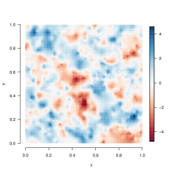
(a) True

(b) fullGP

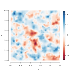
(c) Latent NNGP

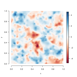
(d) Conjugate Latent NNGP

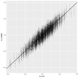
(e) CIs of w from fullGP

(f) CIs of w from Conjugate Latent NNGP

Figure 1: Interpolated maps of (a) the true generated surface, the posterior means of the spatial latent process $w(s)$ for (b) the full Gaussian Process (Full GP), (c) the latent NNGP and (d) the conjugate latent NNGP. The 95% confidence intervals for $w$ from (e) the full GP and (f) the conjugate latent NNGP. The models in (c), and (d) were all fit using $m=10$ nearest neighbors.

The recovered spatial residual surfaces are almost indistinguishable, and are comparable to the true interpolated surface of $w(s)$. Notice that the posterior mean of $w$ of the conjugate latent NNGP model can be theoretically calculated by the $\hat{\gamma}$ in (16). Thus the posterior samples of the latent process $w$ is only required for measuring uncertainty. Figure 1f provides the 95% confidence interval for all latent process $w$ from the conjugate latent NNGP model. There are 955 out of 1000 95% confidence intervals successfully include the true value. This is comparable to the full Gaussian process based model (fig 1e) which has 946 out of 1000 95% confidence intervals covering the true value.

5 Sea surface temperature analysis

Global warming continues to be an ongoing concern among scientists. In order to develop conceptual and predictive global models, NASA monitors temperature and other atmospheric properties of the Earth regularly by two Moderate Resolution Imaging Spectroradiometer (MODIS) instruments in Aqua and Terra platforms. There is an extensive global satellite-based database processed and maintained by NASA. Details of the data can be found in http://modis-atmos.gsfc.nasa.gov/index.html. In particular, inferring on processes generating sea surface temperatures (SST) are of interest to atmospheric scientists studying exchange of heat, momentum, and water vapor between the atmosphere and ocean. Our aforementioned development will enable scientists to analyze large spatially-indexed datasets using a Bayesian geostatistical model easily implementable on modest computing platforms.

Model-based inference is obtained rapidly using the conjugate latent NNGP model and, based on simulation studies, will be practically indistinguishable from MCMC-based output from more general NNGP specification. The dataset we analyze here consists of 2,827,252 spatially indexed observations of sea surface temperature (SST) collected between June 18-26, 2017, the data covers the ocean from longitude -140^∘ to ^∘0 and from latitude 0^∘ to 60^∘. Among the 2,827,252 observations, $n=2,544,527$ (90%) were used for model fitting and the rest were withheld to assess predictive performance of the candidate models. Figure 3a depicts an interpolated map of the observed SST records over training locations. The temperatures are color-coded from shades of blue indicating lower temperatures, primarily seen in the higher latitudes, to shades of red indicating high temperatures. The missing data are colored by yellow and the gray part refers to land. To understand trends across the coordinates, we used sinusoidally projected coordinates (scaled to 1000km units) as explanatory variables. The sinusoidal projection is a popular equal-area projection [see, e.g., ¹ or page 10 in ³]. We compare the Euclidean distances computed from a sinusoidal projection and the spherical or geodesic distance over the study domain by checking the two distances for 4000 pairs of locations randomly selected from the observed location set. The Q-Q plot (figure 2) shows that the Euclidean distance based on sinusoidal projects serves as a good measure of distance over the study domain. An exponential spatial covariance function with sinusoidally projected distance was used for the model. Further model specifications included non-informative flat priors for the intercept and regression coefficients, inverse-gamma priors for $\tau^{2}$ and $\sigma^{2}$ with shape parameter $2$ and scale parameter equaling the respective estimates from an empirical variogram.

We fit the conjugate Bayesian model with fixed $\phi$ and $\delta^{2}$ using the algorithm 1 in Section 3.3with $m=10$ nearest neighbors. We implement Algorithm 2 to choose the values of $\{\phi,\delta^{2}\}$ at $\phi=7$, $\delta^{2}=0.001$.

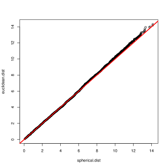
Figure 2: The Q-Q plot of the euclidean distance v.s. the spherical distance of 4000 pairs of observed locations over the study domain of the SST analysis. The red line is the 45 degree line

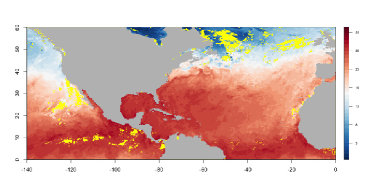
(a) Observed SST over locations for training

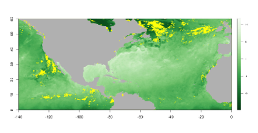
(b) Posterior mean of $w$ over locations for training by Conjugate latent NNGP

(c) Observed SST over locations for testing

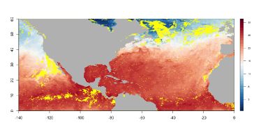
(d) Posterior mean of SST over locations for testing

Figure 3: Notes: (a) Observed SST over locations for training (b) Posterior mean of $w$ over locations for training by Conjugate latent NNGP (c) Posterior mean of SST over locations for testing (d) Posterior mean of SST over locations for testing The land is colored by gray, locations in the ocean without observations are colored by yellow.

Figures 3b shows the posterior means for the latent process of the conjugate latent NNGP model. The temperatures are color-coded from light green indicating high temperatures to dark of green indicating low temperatures. The map of the latent process $w$ indicates lower temperature on the east coast and higher temperature on the west coast. At the same time, we observed high temperture at center of the map. These features coincide with the ocean current, suggesting that the ocean current plays an important role in the sea surface temperature.

Parameter estimates along with their estimated 95% credible intervals and performance metrics for candidate models are shown in Table 2.

Table 2: Real data analysis summary table. Parameter Posterior summary mean (2.5, 97.5) percentiles

	Non-spatial	Conjugate latent NNGP
$\beta_{0}$	31.92(31.91, 31.92)	31.43 (31.28, 31.59)
$\beta_{1}$	0.12 (0.12, 0.12)	0.07 (0.05, 0.09)
$\beta_{2}$	-3.07 (-3.07, -3.07)	-3.03 (-3.08, -2.99)
$\sigma^{2}$	–	3.95 (3.94, 3.95)
$\phi$	–	7.00
$\tau^{2}$	11.44 (11.43, 11.46)	3.95$e^{-3}$ (3.94$e^{-3}$, 3.95$e^{-3}$)
RMSPE	3.39	0.31

The RMSPE for a non-spatial linear regression model, conjugate latent NNGP model were 1.13, 0.31, respectively. Compared to the spatial models, the non-spatial models have substantially higher values of RMSPE, which suggest that coordinates alone does not adequately capture the spatial structure of SST. The fitted SST map over the withheld locations (Fig 3d) using conjugate latent NNGP model is almost indistinguishable from the real SST map (Fig 3c). All the inference from the conjugate latent NNGP model are based on 300 samples. The sampling process took 2367 seconds. In average, the posterior mean of the latent process $w$ can be obtained within 20 seconds.

6 Conclusions and Future Work

This article has attempted to address some practical issues encountered by scientists and statisticians in the hierarchical modeling and analysis for very large geospatial datasets. Building upon some recent work on nearest-neighbor Gaussian processes for massive spatial data, we build conjugate Bayesian spatial regression models and propose strategies for rapidly deliverable inference on modest computing environments equipped with user-friendly and readily available software packages. In particular, we have demonstrated how judicious use of a conjugate latent NNGP model can be effective for estimation and uncertainty quantification of latent (underlying) spatial processes. This provides an easily implementable practical alternative to computationally onerous Bayesian computing approaches. All the computations done in the paper were implemented on a standard desktop using R and Stan. The article intends to contribute toward innovations in statistical practice rather than novel methodologies.

The subsequent research of speeding up Algorithm 1 will include the following two aspects. Firstly, the speed of convergence of the regular CG algorithm to the solution of a symmetric positive definite linear system $Ax=b$ depends on the condition number of the matrix $A$. In practice, a preconditioned CG is much more beneficial. Preconditioning of the CG method in Algorithm 1 is achieved by using a symmetric positive definite preconditioner matrix, say $M=LL^{\top}$, to solve $\tilde{A}\tilde{x}=\tilde{b}$, where $\tilde{A}=L^{-1}AL^{-\top}$ and $\tilde{b}=L^{-1}b$. The solution for $Ax=b$ is then obtained as $x=L^{-\top}\tilde{x}$. The preconditioner should be chosen carefully. It should enjoy high memory efficiency and also ensure that $\kappa(\tilde{A})$ is close to 1, where $\kappa(\cdot)$ denotes the condition number of a matrix. Without these conditions, the benefits of preconditioning will not be evident and further investigations are needed to specify efficient preconditioners for modifying Algorithm 1. The second aspect is parallel computing. The posterior samples generated by Algorithm 1 are independent, allowing the possibility of generating them simultaneously. One could explore the use of different parallel programming paradigms such as message parsing interfaces and GPUs to dramatically reduce the sampling times in Algorithm 1.

It is important to recognize that the conjugate Bayesian models outlined here are not restricted to the NNGP. Any spatial covariance structure that leads to efficient computations can, in principle, be used. There are a number of recently proposed approaches that can be adopted here. These include, but are not limited to, multi-resolution approaches e.g., ²⁷, ²⁶, ²¹, covariance tapering and its use in full-scale approximations e.g., ¹³, ³¹, ²⁰, and stochastic partial differential equation approximations ²⁴, among several others see, e.g., ² and references therein.

With regard to the NNGP specifically, our choice was partially dictated by its easy implementation in R using the spNNGP package and in Stan as described in http://mc-stan.org/users/documentation/case-studies/nngp.html. The NNGP is built upon a very effective likelihood approximation ³⁶, ³⁴, which has also been explored recently by several authors in a variety of contexts ³⁵, ¹⁸. ¹⁸ provides empirical evidence about Vecchia’s approximation outperforming other alternate methods, but also points out some optimal methods for permuting the order of the spatial locations before constructing the model. His methods for choosing the order of the locations can certainly be executed prior to implementing the models proposed in this article. Finally, an even more recent article by ²² proposes further extensions of the Vecchia approximation, but its practicability for massive datasets on modest computing environments with easily available software packages is yet to be ascertained.

Supplementary Material

All computer programs implementing the examples in this article can be found in the public domain and downloaded from https://github.com/LuZhangstat/ConjugateNNGP.

References

- Banerjee 2005 Banerjee, S., 2005: On geodetic distance computations in spatial modeling. Biometrics, 61, no. 2, 617–625.
- Banerjee 2017 — 2017: High-dimensional bayesian geostatistics. Bayesian Analysis, 12, 583–614.
- Banerjee et al. 2014 Banerjee, S., B. P. Carlin, and A. E. Gelfand, 2014: Hierarchical modeling and analysis for spatial data. Crc Press.
- Banerjee and Roy 2014 Banerjee, S. and A. Roy, 2014: Linear algebra and matrix analysis for statistics. CRC Press.
-
Bates and Eddelbuettel 2013
Bates, D. and D. Eddelbuettel, 2013: Fast and elegant numerical linear algebra
using the RcppEigen package. Journal of Statistical Software, 52, no. 5, 1–24.
URL http://www.jstatsoft.org/v52/i05/ - Bishop 2006 Bishop, C., 2006: Pattern Recognition and Machine Learning. Springer-Verlag, New York, NY.
- Chilés and Delfiner 1999 Chilés, J. and P. Delfiner, 1999: Geostatistics: Modeling Spatial Uncertainty. John Wiley: New York.
- Cressie and Wikle 2015 Cressie, N. and C. K. Wikle, 2015: Statistics for spatio-temporal data. John Wiley & Sons.
-
Datta et al. 2016a
Datta, A., S. Banerjee, A. O. Finley, and A. E. Gelfand, 2016a:
Hierarchical nearest-neighbor gaussian process models for large
geostatistical datasets. Journal of the American Statistical
Association, 111, 800–812.
URL http://dx.doi.org/10.1080/01621459.2015.1044091 -
Datta et al. 2016b
Datta, A., S. Banerjee, A. O. Finley, N. A. S. Hamm, and M. Schaap,
2016b: Non-separable dynamic nearest-neighbor gaussian process
models for large spatio-temporal data with an application to particulate
matter analysis. Annals of Applied Statistics, 10, 1286–1316.
URL http://dx.doi.org/10.1214/16-AOAS931 -
Finley et al. 2017a
Finley, A., A. Datta, and S. Banerjee, 2017a: spNNGP: Spatial
Regression Models for Large Datasets using Nearest Neighbor Gaussian
Processes. R package version 0.1.1.
URL https://CRAN.R-project.org/package=spNNGP - Finley et al. 2017b Finley, A. O., A. Datta, B. C. Cook, D. C. Morton, H. E. Andersen, and S. Banerjee, 2017b: Applying nearest neighbor gaussian processes to massive spatial data sets: Forest canopy height prediction across tanana valley alaska. arXiv preprint arXiv:1702.00434.
- Furrer et al. 2006 Furrer, R., M. G. Genton, and D. Nychka, 2006: Covariance tapering for interpolation of large spatial datasets. Journal of Computational and Graphical Statistics, 15, 503–523.
- Gelfand et al. 2010 Gelfand, A. E., P. Diggle, P. Guttorp, and M. Fuentes, 2010: Handbook of spatial statistics. CRC press.
- Gelman et al. 2013 Gelman, A., J. B. Carlin, H. S. Stern, D. B. Dunson, A. Vehtari, and D. B. Rubin, 2013: Bayesian Data Analysis, 3rd Edition. Chapman & Hall/CRC Texts in Statistical Science, Chapman & Hall/CRC.
- Gneiting and Raftery 2007 Gneiting, T. and A. E. Raftery, 2007: Strictly proper scoring rules, prediction, and estimation. Journal of the American Statistical Association, 102, no. 477, 359–378.
- Golub and Van Loan 2012 Golub, G. H. and C. F. Van Loan, 2012: Matrix Computations, 4th Edition. Johns Hopkins University Press.
- Guinness 2016 Guinness, J., 2016: Permutation methods for sharpening gaussian process approximations. arXiv preprint arXiv:1609.05372.
-
Heaton et al. 2017
Heaton, M., A. Datta, A. Finley, R. Furrer, R. Guhaniyogi, F. Gerber,
D. Hammerling, M. Katzfuss, F. Lindgren, D. Nychka, and A. Zammit-Mangion,
2017: Methods for analyzing large spatial data: A review and comparison. arXiv:1710.05013.
URL https://arxiv.org/abs/1710.05013 - Katzfuss 2013 Katzfuss, M., 2013: Bayesian nonstationary modeling for very large spatial datasets. Environmetrics, 24, 189—200.
-
Katzfuss 2017
— 2017: A multi-resolution approximation for massive spatial datasets. Journal of the American Statistical Association, 112, 201–214,
doi:10.1080/01621459.2015.1123632.
URL http://dx.doi.org/10.1080/01621459.2015.1123632 - Katzfuss and Guinness 2017 Katzfuss, M. and J. Guinness, 2017: A general framework for vecchia approximations of gaussian processes. arXiv preprint arXiv:1708.06302.
- Lauritzen 1996 Lauritzen, S. L., 1996: Graphical Models, Clarendon Press, Oxford, United Kingdom.
-
Lindgren et al. 2011
Lindgren, F., H. Rue, and J. Lindstrom, 2011: An explicit link between gaussian
fields and gaussian markov random fields: the stochastic partial differential
equation approach. Journal of the Royal Statistical Society: Series B
(Statistical Methodology), 73, no. 4, 423–498,
doi:10.1111/j.1467-9868.2011.00777.x.
URL http://dx.doi.org/10.1111/j.1467-9868.2011.00777.x - Murphy 2012 Murphy, K., 2012: Machine Learning: A probabilistic perspective. The MIT Press, Cambridge, MA.
-
Nychka et al. 2015
Nychka, D., S. Bandyopadhyay, D. Hammerling, F. Lindgren, and S. Sain, 2015: A
multiresolution gaussian process model for the analysis of large spatial
datasets. Journal of Computational and Graphical Statistics, 24, no. 2, 579–599, doi:10.1080/10618600.2014.914946.
URL http://dx.doi.org/10.1080/10618600.2014.914946 - Nychka et al. 2002 Nychka, D., C. Wikle, and J. A. Royle, 2002: Multiresolution models for nonstationary spatial covariance functions. Statistical Modelling, 2, no. 4, 315–331.
-
Ribeiro Jr and Diggle 2012
Ribeiro Jr, P. J. and P. J. Diggle, 2012: geoR: a package for
geostatistical analysis. R package version 1.7-4.
URL https://cran.r-project.org/web/packages/geoR -
Rue and Held 2005
Rue, H. and L. Held, 2005: Gaussian Markov Random Fields : Theory and
Applications, Chapman & Hall/CRC, Boca Raton, FL. Monographs on
statistics and applied probability.
URL http://opac.inria.fr/record=b1119989 -
Rue et al. 2009
Rue, H., S. Martino, and N. Chopin, 2009: Approximate bayesian inference for
latent gaussian models by using integrated nested laplace approximations.
Journal of the Royal Statistical Society: Series B (Statistical
Methodology), 71, no. 2, 319–392,
doi:10.1111/j.1467-9868.2008.00700.x.
URL http://dx.doi.org/10.1111/j.1467-9868.2008.00700.x - Sang and Huang 2012 Sang, H. and J. Z. Huang, 2012: A full scale approximation of covariance functions for large spatial data sets. Journal of the Royal Statistical society, Series B, 74, 111–132.
-
Stan Development Team 2016
Stan Development Team, 2016: RStan: the R interface to Stan. R
package version 2.14.1.
URL http://mc-stan.org/ - Stein 1999 Stein, M. L., 1999: Interpolation of Spatial Data: Some Theory for Kriging, Springer. Firstnd ed.
- Stein et al. 2004 Stein, M. L., Z. Chi, and L. J. Welty, 2004: Approximating likelihoods for large spatial data sets. Journal of the Royal Statistical society, Series B, 66, 275–296.
-
Stroud et al. 2017
Stroud, J. R., M. L. Stein, and S. Lysen, 2017: Bayesian and maximum likelihood
estimation for gaussian processes on an incomplete lattice. Journal of
Computational and Graphical Statistics, 26, 108–120.
URL http://dx.doi.org/10.1080/10618600.2016.1152970 - Vecchia 1988 Vecchia, A. V., 1988: Estimation and model identification for continuous spatial processes. Journal of the Royal Statistical society, Series B, 50, 297–312.
- Yeniay and Goktas 2002 Yeniay, O. and A. Goktas, 2002: A comparison of partial least squares regression with other prediction methods. Hacettepe Journal of Mathematics and Statistics, 31, no. 99, 99–101.