Learning random-walk label propagation
for weakly-supervised semantic segmentation

Abstract

Large-scale training for semantic segmentation is challenging due to the expense of obtaining training data for this task relative to other vision tasks. We propose a novel training approach to address this difficulty. Given cheaply-obtained sparse image labelings, we propagate the sparse labels to produce guessed dense labelings. A standard CNN-based segmentation network is trained to mimic these labelings. The label-propagation process is defined via random-walk hitting probabilities, which leads to a differentiable parameterization with uncertainty estimates that are incorporated into our loss. We show that by learning the label-propagator jointly with the segmentation predictor, we are able to effectively learn semantic edges given no direct edge supervision. Experiments also show that training a segmentation network in this way outperforms the naive approach.

1 Introduction

Figure 1: Overview of proposed training method.

We consider the task of semantic segmentation, which is to learn a predictor capable of accurately assigning a semantic label to each pixel in an image. As with many other popular vision problems, convolutional neural nets (CNNs) have emerged as the leading tool to solve semantic segmentation problems, in part due to their ability to leverage large datasets effectively. However, datasets for semantic segmentation remain orders of magnitude smaller than for tasks such as classification and detection, due chiefly to the much higher annotation expense of this task.

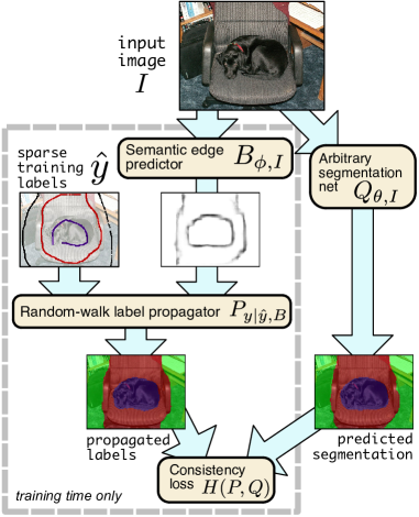
To ease the annotation burden, and in line with previous work [1, 11], we propose a method for training CNN-based semantic segmentation networks given sparse annotations, such as the scribbles depicted in Fig. 1, which also depicts our proposed training strategy. The idea of our method is to learn mutually-consistent networks for propagating the sparse labels to unlabeled points, and predicting the true labeling given the image alone. Optimizing a mutual-consistency objective obviates the need for dense (or, fully-labeled) supervision. A key innovation of our approach is proposing to use a specific, probabilistic model of sparse label propagation that is a differentiable function of semantic boundary predictions. As it is differentiable, minimizing our loss via gradient-based methods results in simultaneous learning of an image-to-semantic-boundary predictor and an image-to-semantic-segmentation predictor, despite having no direct observations of semantic edges.

Our method is comparable to recent work by Lin et al. [11], which proposes alternating between propagating sparse labels using a CRF defined over superpixels, and training a CNN to predict the labels thus inferred. A disadvantage of this approach relative to ours is that [11] employs a notion of label smoothness that is non-adaptive: specifically, it is assumed that labels are constant within superpixels, and the CRF binary potentials are not learned. This ultimately places an artificial upper bound on the accuracy of the training data observed by the CNN—an upper bound that never improves as more data is collected. By contrast, by expressing label propagation in terms of a learned semantic boundary predictor, we are able to learn a concept of label propagation that is entirely data-driven, enabling our method to scale fully with the data. Furthermore, the probabilistic nature of our label propagation method allows us to obtain uncertainty estimates that are directly incorporated into our learning process, mitigating the possibilty of training on propagated labels that are incorrect.

A crucial technical component of our approach is defining the label propagation process in terms of random-walk hitting probabilities [6], which enables efficient inference and gradient-based learning. For this reason, we refer to our approach as RAWKS, a contraction of RAndom-walk WeaKly-supervised Segmentation.

2 Method

Table 1: Notation

$X\subset\mathbb{Z}^{2}$	set of all pixel locations
$\hat{}X\subset X$	set of labeled pixels
$\mathcal{L}$	set of semantic labels
$y\mathrel{\mathop{\mathchar 58\relax}}X\rightarrow\mathcal{L}$	a semantic labeling function
$\hat{y}\mathrel{\mathop{\mathchar 58\relax}}\hat{}X\rightarrow\mathcal{L}$	a sparse labeling
$I$	a generic image
$\theta,\phi$	predictor parameters
$\Delta^{n}$	$n$-dim. probability simplex
$Q_{\theta,I}\mathrel{\mathop{\mathchar 58\relax}}X\rightarrow\Delta^{|\mathcal{L}|}$	label predictor
$B_{\phi,I}\mathrel{\mathop{\mathchar 58\relax}}X\rightarrow\mathbb{R}^{+}$	boundary predictor
$\Xi\subset\mathbb{Z}^{+}\rightarrow X$	set of paths across image
$\xi\in\Xi$	a random walk
$\tau\mathrel{\mathop{\mathchar 58\relax}}\Xi\rightarrow\mathbb{Z}^{+}$	path stopping time
$P_{a\mid b}\in\Delta$	distribution of $a$ given $b$
$\delta_{i}\in\{0,1\}^{|\delta_{i}|}\cap\Delta^{|\delta_{i}|}$	Kronecker delta vector
$H(p)$	Shannon entropy of $p$
$H(p,q)$	cross-entropy of $p,q$
$\textrm{KL}(p\;\|\;q)$	KL-divergence of $p,q$

Given densely labeled training images, typical approaches for deep-learning-based semantic segmentation minimize the following cross-entropy loss [12, 3]:

$$\min_{\theta\in\Theta}\sum_{x\in X}H(\delta_{y(x)}\,,Q_{\theta,I}(x)),$$ (1)

where $\delta_{y(x)}\in\Delta^{|\mathcal{L}|}$ is the indicator vector of the ground truth label $y(x)$ and $Q_{\theta,I}(x)$ is a label distribution predicted by a CNN with parameters $\theta$ evaluated on image $I$ at location $x$. See Table 1 for notation. In our case, dense labels $y(x)$ are not provided: we only have labels $\hat{y}$ provided at a subset of points $\hat{}X$. Our solution is to simultaneously infer the dense labeling $y$ given the sparse labeling $\hat{y}$ and use the inferred labeling to train $Q$. To achive this, we propose to train our predictor to minimize the following loss:

$$\min_{\theta,\phi}\sum_{x\in X}H(P_{y(x)\mid\hat{y},B_{\phi,I}}\,,Q_{\theta,I}(x)).$$ (2)

Here, $Q$ is a predictor of the same form as before, while $P_{y(x)\mid\hat{y},B_{\phi,I}}$ is a predicted label distribution at $x$, conditioned on predicted semantic boundaries $B_{\phi,I}$ and the sparse labels. $B_{\phi,I}$ is assumed to be a nonnegative-valued CNN-based boundary predictor, in a similar vein as [2, 14]. See Fig. 1 for a graphical overview of our model.

The key to our method is the definition of the propagated label distributions $P_{y\mid\hat{y},B_{\phi,I}}$. As in prior work on interactive segmentation [6], we define these distributions in terms of random-walk hitting probabilities, which can be computed analytically, and which allows us to compute the derivatives of the propagated label probabilities with respect to the predicted boundaries. This enables us to minimize (2) by pure backpropagation, without tricks such as the alternating optimization methods employed in prior weakly-supervised segmentation methods [4, 11].

To elaborate, we first define the set of all 4-connected paths on the image that end at the first labeled point encountered:

$$\Xi=\{(\xi_{0},\xi_{1},\dots, \xi_{\tau(\xi)})\mid\forall t,\xi_{t}\in X,\|\xi_{t+1}-\xi_{t}\|_{1}=1,$$

$$\xi_{\tau(\xi)}\in\hat{}X,\forall t^{\prime}<\tau(\xi)\,,\xi_{t^{\prime}}\notin\hat{}X\}.$$ (3)

We now assign each path $\xi\in\Xi$ a probability that decays exponentially as it crosses boundaries:

$$P(\xi)\propto\exp\left(-\sum_{t=0}^{\tau(\xi)-1}B_{\phi,I}(\xi_{t})\right)\frac{1}{4}^{\tau(\xi)},$$ (4)

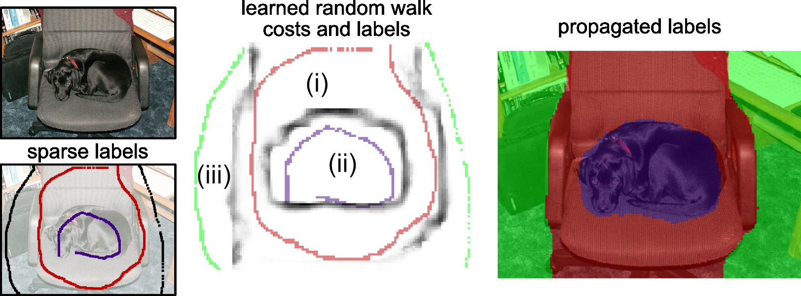
where $B_{\phi,I}$ is assumed to be a nonnegative boundary score prediction. High- and low-probability paths under this model are illustrated in Fig. 2(b). Given sparse labels $\hat{y}$, the probability that a pixel $x$ has label $y^{\prime}$ is then defined as the probability that a path starting at $x$ eventually hits a point labeled $y^{\prime}$, given the distribution over paths (4):

$$P_{y(x)\mid\hat{y},B_{\phi,I}}(y^{\prime})=P(\{\xi\in\Xi\mid\xi_{0}=x,\hat{y}(\xi_{\tau(\xi)})=y^{\prime}\}).$$ (5)

This quantity can be computed efficiently by solving a sparse linear system, as described in Sec. 2.2. The random-walk model is illustrated in Fig. 2(a). Any pixel in the region labeled (ii), for example, is very likely to be labeled dog instead of chair or background, because any path of significant probability starting in (ii) will hit a pixel labeled dog before it hits a pixel with any other label.

(a)

(b)

Figure 2: Illustration of random-walk-based model for defining label probabilities based on boundaries and sparse labels.

To recap, the overall architecture of our method is summarized in Fig. 1. At training time, an input image is passed to an arbitrary segmentation predictor $Q_{\theta,I}$ and an arbirtary semantic edge predictor $B_{\phi,I}$. The semantic edge predictions and sparse training labels $\hat{y}$ are passed to a module that computes propagated label probabilities $P_{y\mid\hat{y},B}$ using the random-walk model described above. The propagated label probabilities $P$ and the output of the predictor $Q$ are then passed to a cross-entropy loss $H(P,Q)$, which is minimized in the parameters $\theta$ and $\phi$ via backpropagation. At test time, $Q$ is evaluated and used as the prediction. $P$ is not evaluated at test time, since labels are not available.

2.1 Probabilistic justification

Figure 3: Independence assumptions as a graphical model

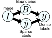
The proposed loss function (2) arises from a natural probabilistic extension of (1) to the case where dense labels are unobserved. Specifically, we consider marginalizing (1) over the unobserved dense labels, given the observed sparse labels. This requires us to define $P(y\mid\hat{y},I)$. We submit that a natural way to do so is to introduce a new variable $B$ representing the image’s semantic boundaries. This results in the proposed graphical model in Fig. 3 to represent the independence structure of $y,\hat{y},B,I$.

It is then straightforward to show that (2) is equivalent to marginalizing (1) with respect to a certain distribution $P(y\mid\hat{y},I)$, after making a few assumptions. First, the conditional independence structure depicted in Fig. 3 is assumed. $y(x)$ and $y(x^{\prime})$ are assumed conditionally independent given $\hat{y},B,$ $\forall x\neq x^{\prime}\in X$, which allows us to specify $P(y\mid\hat{y},B)$ in terms of marginal distributions and simplifies inference. Finally, $B$ is assumed to be a deterministic function of $I$, defined via parameters $\phi$.

We note that the conditional independence assumptions made in Fig. 3 are significant. In particular, $y$ is assumed independent of $I$ given $\hat{y}$ and $B$. This essentially implies that there is at least one label for each connected component of the true label image, since knowing the underlying image usually does give us information as to the label of unlabeled connected components. In practice, strictly labeling every connected component is not necessary. However, training data that egregiously violates this assumption will likely yield poor results.

2.2 Random-walk inference

Key to our method is the efficient computation of the random-walk hitting probabilities (5). It is well-known that such probabilities can be computed efficiently via solving linear systems [6]. We briefly review this result here.

The basic strategy is to compute the partition function $Z_{xl}$, which sums the right-hand-side of (4) over all paths starting at $x$ and ending in a point labeled $l$. We can then derive a dynamic programming recursion expressing $Z_{xl}$ in terms of the same quantity at neighboring points $x^{\prime}$. This recursion defines a set of sparse linear constraints on $Z$, which we can then solve using standard sparse solvers.

We first define $\Xi_{xl}\mathrel{\mathop{\mathchar 58\relax}}=\{\xi\in\Xi\mid\xi_{0}=x,\,\hat{y}(\xi_{\tau(\xi)})=l\}$. $Z_{xl}$ is then defined as

$$Z_{xl}\mathrel{\mathop{\mathchar 58\relax}}=\sum_{\xi\in\Xi_{xl}}\exp\left(-\sum_{t=0}^{\tau(\xi)-1}B_{\phi,I}(\xi_{t})\right)\frac{1}{4}^{\tau(\xi)}.$$ (6)

The first term in the inner sum can be factored out by introducing a new summation over the four nearest neighbors of $x$, denoted $x^{\prime}\sim x$, easily yielding the recursion

$$Z_{xl} =\frac{1}{4}e^{-B_{\phi,I}(x)}\sum_{\begin{subarray}{c}x^{\prime}\sim x,\\ \xi\in\Xi_{x^{\prime}l}\end{subarray}}\frac{1}{4}^{\tau(\xi)}e^{-\sum_{t=0}^{\tau(\xi)-1}B_{\phi,I}(\xi_{t})}$$

$$=\frac{1}{4}e^{-B_{\phi,I}(x)}\sum_{x^{\prime}\sim x}Z_{x^{\prime}l}.$$ (7)

Boundary conditions must also be considered in order to fully constrain the solution. Paths exiting the image are assumed to have zero probability: hence, $Z_{xl}\mathrel{\mathop{\mathchar 58\relax}}=0,\,\forall x\notin X$. Paths starting at a labeled point $x\in\hat{}X$ immediately terminate with probability 1; hence, $Z_{xl}\mathrel{\mathop{\mathchar 58\relax}}=1,\,\forall x\in\hat{}X$. Solving this system yields a unique solution for $Z$, from which the desired probabilities are computed as

$$P_{y(x)\mid\hat{y},B_{\phi,I}}(y^{\prime})=\frac{Z_{xy^{\prime}}}{\sum_{l\in\mathcal{L}}Z_{xl}}.$$ (8)

2.3 Random-walk backpropagation

In order to apply backpropagation, we must ultimately compute the derivative of the loss with respect to a change in the boundary score prediction $B_{\phi,I}$. Here, we focus on computing the derivative of the partition function $Z$ with respect to the boundary score $B$, the other steps being trivial.

Since computing $Z$ amounts to solving a linear system, this turns out to be fairly simple. Let us write the constraints (7) in matrix form $Az=b$, such that $A$ is square, $z_{i}\mathrel{\mathop{\mathchar 58\relax}}=Z_{x_{i}}$ (assigning a unique linear index $i$ to each $x_{i}\in X$, and temporarily omitting the dependence on $l$), and the $i$th rows of $A,b$ correspond to the constraints $C_{i}Z_{x_{i}}=\sum_{x^{\prime}\sim x_{i}}Z_{x^{\prime}}$, $Z_{x_{i}}=0$, or $Z_{x_{i}}=1$ (as appropriate), where $C_{i}\mathrel{\mathop{\mathchar 58\relax}}=\exp(B_{\phi,I}(x_{i}))$. Let us consider the effect of adding a small variation $\epsilon V$ to $A$, and then re-solving the system. It can be shown that

$$(A+\epsilon V)^{-1}b=z-\epsilon A^{-1}Vz+O(\epsilon^{2}).$$ (9)

Substituting the first-order dependence on $V$ into a Taylor expansion of the loss $L$ yields:

$$L((A+\epsilon V)^{-1}b) =L(z)-\left<\mathinner{\dfrac{\operatorname{d\!}{}L}{\operatorname{d\!}{z}}},\epsilon A^{-1}Vz\right>+O(\epsilon^{2})$$

$$=L(z)-\left<A^{-1\intercal}\mathinner{\dfrac{\operatorname{d\!}{}L}{\operatorname{d\!}{z}}}z^{\intercal},\epsilon V\right>+O(\epsilon^{2}).$$

A first-order variation of $C_{i}$ corresponds to $V_{i}=-\delta_{ii}$, which implies that

$$\mathinner{\dfrac{\operatorname{d\!}{}L}{\operatorname{d\!}{C_{i}}}}=\left(A^{\intercal-1}\mathinner{\dfrac{\operatorname{d\!}{}L}{\operatorname{d\!}{z}}}\right)_{i}z_{i}.$$ (10)

In summary, this implies that computing the loss derivatives with respect to the boundary score can be implemented efficiently by solving the sparse adjoint system $A^{\intercal}\dfrac{\operatorname{d\!}{}L}{\operatorname{d\!}{C}}=\dfrac{\operatorname{d\!}{}L}{\operatorname{d\!}{z}}$, and multiplying the result pointwise by the partition function $z$, which in turn allows us to efficiently incorporate sparse label propagation as a function of boundary prediction into an arbitrary deep-learning framework.

2.4 Uncertainty-weighting the loss

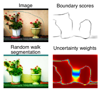
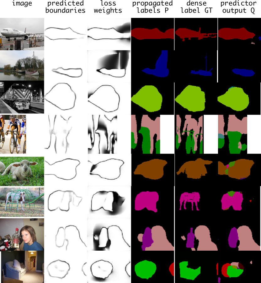
An advantage of our method over prior work is that the random-walk method produces a distribution over dense labelings $P_{y\mid\hat{y},B_{\phi,I}}$ given sparse labels, as opposed to a MAP estimate. These uncertainty estimtates can be used to down-weight the loss in areas where the inferred labels may be incorrect, as illustrated in Fig. 4. In this example, the boundary predictor failed to correctly predict parts of object boundaries. In the vicinity of these gaps, the label distribution is uncertain, and the MAP estimate is incorrect. However, we can mitigate the problem by down-weighting the loss proportional to the uncertainty estimate.

More concretely, we actually minimize the following modification of the loss (2):

$$\sum_{x\in X}w(x)\textrm{KL}(P_{y(x)\mid\hat{y},B_{\phi,I}}\;\|\;Q_{\theta,I}(x))+H(P_{y(x)\mid\hat{y},B_{\phi,I}}),$$ (11)

where we define $w(x)\mathrel{\mathop{\mathchar 58\relax}}=\exp(-\alpha H(P_{y(x)\mid\hat{y},B_{\phi,I}}))$, for some fixed parameter $\alpha$. This loss reduces to (2) for the case $w(x)=1$. Although the KL component of the loss can be avoided by increasing the prediction entropy, the explicit entropy regularization term prevents trivial solutions of very large entropy everywhere.

Figure 4: Visualization of loss uncertainty weights (blue = low weight, red = high weight)

3 Related work

The method most comparable to ours is the work of Lin et al. [11]. In contrast to [11], our method features fully-differentiable, gradient-based training (as opposed to alternating optimization); we learn an inductive rule for predicting boundaries and propagating labels, as opposed to using non-adaptive superpixels and a CRF with non-adaptive binary potentials, which enables us to adapt to large datasets in a data-driven way; and we employ a probabilistic notion of label propagation that enables us to define an uncertainty-weighted loss that mitigates the possibilty of training on propagated labels that are incorrect. Another notable method in the same vein as [11] is the BoxSup method [4], which also employs alternating optimization, but uses bounding-box annotations as weak supervision.

Our method was initially inspired by [1], which introduced the idea of training on what we refer to here as sparse labels as a source of weak supervision. Instead of attempting to directly propagate labels, as we do, that method leverages a notion of objectness to mitigate overfitting. A few other works have proposed different modes of weak supervision for segmentation. Notably, [15] and [13] both model weak supervision as imposing linear constraints to be satisfied by the predictor, resulting in models trained by alternating optimization. Our method can be viewed from a similar perspective, since we also impose our weak supervision via linear constraints (7); however, our constraints explicitly model the process of spatial label propagation, whereas the constraints proposed in [15, 13] model only aggregate statistics over regions, and hence make no provision for learning boundaries as we do in this work. Furthermore, our model is differentiable and can be optimized via gradient-based methods.

To the extent that it learns semantic edges with a CNN, our method is similar to previous works such as [14], which also learns semantic edges using a CNN. However, [14] achieves this using direct supervision of edges—which we do not require—and does not jointly train a semantic labeler, as we do. Learning edges with a weaker form of edge supervision is proposed in [10]; however, this method relies on a combination of heuristic boundary detectors and bounding boxes for supervision. To reiterate, our method works without any heuristic source of boundaries as input.

Another vein of prior work relates to some form of joint reasoning about boundaries and segments. Most prominently, random walks were previously applied to interactive segmentation in [6]. However, that work did not consider learning these random walks by learning boundary scores, as we do, nor did it consider the task of semantic image segmentation in general. More recently, [2] proposed a method to jointly learn semantic edges and a CNN-based semantic labeler in an gradient-based learning framework. However, their method applies only to the strong-supervision case, and cannot leverage sparse annotations of the kind we employ here.

4 Experiments

We implemented RAWKS in the Caffe [9] framework. The semantic-boundary-prediction network $B_{\phi,I}$ and the semantic-segmentation network $Q_{\theta,I}$ were both implemented as fully-convolutional CNNs, based on the same ResNet-101 [8] architecture. The final average-pooling and fully-connected layers were removed, and features from the last resulting layer were upsampled and combined with intermediate-layer features to produce a 4x-downsampled output for both the semantic boundary and label predictions. Both networks were initialized from a model trained for classification on the ImageNet 2012 dataset. We applied no data augmentation techniques in training any of the methods.

RAWKS was trained on the publicly available scribble annotations provided by [11]. We used the same training and validation splits as [11], for both the PASCAL VOC 2012 and PASCAL CONTEXT datasets: for VOC, the validation set consisted of the VOC 2012 validation set, while the training set consisted of all other images labeled in either the VOC 2012 dataset or the PASCAL Semantic Boundary dataset [7] (10582 training images, and 1449 validation images). We trained models for each of these datasets independently.

We evaluated the performance of both the semantic-segmentation network $Q$ and the label-propagation network $P$ (propagating the sparse labels given the learned boundaries). To summarize, evaluating the predicted labels $Q$ on the validation set, RAWKS slightly underperformed the published results of [11] on VOC 2012, while slightly outperforming [11] on CONTEXT. Our other major observation was that the propagated labels $P$ on the training set were approximately as accurate as the best possible labeling of a superpixel segmentation of the images.

To elaborate, in Table 2, MIOU refers to the mean-intersection-over-union metric, while w/ CRF refers to the same metric evaluated after post-processing the results with a fully-connected CRF, as in [11]. RAWKS $Q_{\theta,I}$ refers to the evaluation of the predicted labels $Q$ on the validation set given the image alone, after jointly training $P$ and $Q$ via SGD. RAWKS train P,Q then Q also refers to evaluation of $Q$, but with a slightly different training protocol: in this case after jointly training $P$ and $Q$ with SGD, $Q$ was fine-tuned with $P$ fixed. RAWKS training $P_{y\mid\hat{y},B}$, 0% abstain refers to evaluation of $P$ on the training set, given the sparse training labels and learned boundaries $B_{\phi,I}$. RAWKS training $P_{y\mid\hat{y},B}$, 6% abstain consists of the same evaluation, but allowing $P$ to abstain from prediction on 6% of the pixels, which (for this particular model) corresponds to abstaining on all pixels with a confidence score $w(x)$ below 0.5 (c.f. Sec. 2.4). The next section of Table 2 reports baselines: sparse-loss baseline consists of training the same base network $Q$, but using loss (1) (i.e., without $P$), evaluating it only at the sparse locations $\hat{}X$. train on dense ground truth is the result we obtain training our base network $Q$ on the dense ground-truth training data. ScribbleSup refers to the result reported by [11], which we report here verbatim. We note that [11] used a different base segmentation network (DeepLab) than we used in our experiments.

The last section of Table 2 reports statistics for baselines meant to represent best-case performance bounds for a superpixel-based method such as [11]. These were obtained by segmenting the input images using the method [5] (with author-suggested parameters), and labeling the resulting superpixels in different ways. SPOPT corresponds to labeling each superpixel with the majority label from the ground-truth dense segmentation. SPCON differs from SPOPT only on superpixels containing scribble annotations: to these, SPCON assigns the majority label from the scribbles contained within. Train on SPOPT/SPCON refer to training predictors $Q$ using the labelings of SPOPT and SPCON, respectively. These results are interesting for a number of reasons. First, the propagated labelings $P$ that we deduce in the course of training, are nearly as good (VOC) or better (CONTEXT) than the best possible results obtainable using superpixels. Second, we see that training with our propagated labelings $P$ is competitive with training on optimal superpixel labelings. Finally, we emphasize that while the superpixel baselines cannot improve with training data (as they are not trained), our label propagation model is naturally refined as we train on larger datasets.

In relative terms, RAWKS performed better on the CONTEXT dataset, as evidenced in Table 3. One potential reason for this is the greater number of classes for this dataset (60 vs. 21 for VOC), which naturally calls for finer boundaries. Since our method is able to adaptively learn boundaries suited to the task, while [11] uses non-adaptive heuristics to generate superpixels, this may account for the better relative performance of RAWKS in this context. We also hypothesize that it is easier to learn semanic boundaries when there are a greater number of classes, because low-level edges and features become a more informative cue in this case. Surprisingly, our dense ground-truth baseline performed significantly worse than RAWKS; we hypothesize this is due to overfitting, a consequence of the smaller amount of training data and increased number of classes in CONTEXT, exacerbated by our use of the very-deep ResNet model. Joint training of the propagator network $P$ in RAWKS seems to have a regularizing effect that may have prevented overfitting to some extent.

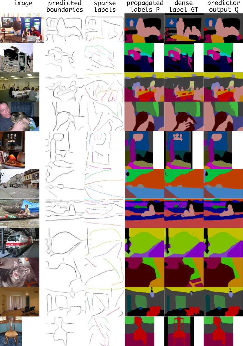
Qualitative validation-set results are shown in Fig. 5 for the VOC 2012 dataset, while CONTEXT training-set results are shown in Fig. 6. The training-set results of Fig. 6 demonstrate that RAWKS is able to deduce high-quality semantic boundaries, thereby producing propagated labelings $P$ that are a close approximation to the ground truth dense labelings (which are not used at training time, to be clear). In the validation-set results of Fig. 5, the loss weights $w(x)$ and propagated labels $P$ are shown in addition to the predictions $Q$—to be clear, these depend on the sparse labels for these specific examples, which were not used to train this model. Here we remark that our semantic boundary predictions also generalize well to the validation set. Although we did not train on these images, we also observe that had we done so, the loss weights would have behaved appropriately, down-weighting the loss in regions where the propagated labels are incorrect. This seems to happen most often in regions with very fine boundaries (such as the mast of the boat and the airplane’s wing), where our limited resolution sometimes causes missed boundaries.

In general, we note that subjectively, resolution seemed to be a limiting factor in the accuracy of our boundary prediction and label propagation steps. We used quarter-resolution outputs (typicaly around 128x96 pixels) for these steps in order to minimize the computational cost of computing random-walk hitting probabilities. An average forward-backwards pass of the entire network took about 1.1 s per image, with about 800 ms of that spent solving for the random-walk hitting probabilities. This layer was implemented using a CPU-based sparse linear system solver, whereas the rest of the network was run on the GPU (an NVIDIA GTX 1080). We anticipate that implementing this layer using GPU operations will allow us to increase the resolution of these critical steps, which will in turn lead to increased prediction accuracy.

Figure 5: Validation set results on VOC 2012 dataset

Method	MIOU	w/ CRF
RAWKS $Q_{\theta,I}$	57.1	60.0
RAWKS train $P,Q$, then $Q$	59.5	61.4
RAWKS training $P_{y\mid\hat{y},B}$, 0% abstain	75.8	.
RAWKS training $P_{y\mid\hat{y},B}$, 6% abstain	81.2	.
Sparse-loss baseline	55.8
Train on dense ground truth	66.3	68.8
ScribbleSup (reported)	.	63.1
Opt. superpixel labels (SPOPT)	83.1	.
Opt. consistent s-p. labels (SPCON)	76.5	.
Train on SPOPT	62.8	.
Train on SPCON	61.1	.

Table 2: Results on VOC 2012 validation set

Method	MIOU	w/ CRF
RAWKS $Q_{\theta,I}$	36.0	37.4
RAWKS training $P_{y\mid\hat{y},B}$, 0% abstain	75.5	.
Sparse-loss baseline	26.6	.
Train on dense ground truth	31.7	32.4
ScribbleSup (reported)	.	36.1
Opt. consistent s-p. labels (SPCON)	70.2	.

Table 3: Results on CONTEXT validation set

Figure 6: Training results on CONTEXT dataset

5 Conclusions

We have presented a novel approach to mitigating the expense of procuring labeled data in semantic segmentation, through a framework that utilizes only sparse clicks or scribbles for training. This has a significant impact on the possibilities for semantic segmentation—for a given dataset, one may obtain competitive labels at a fraction of the cost and conversely, for a given budget, one may obtain labeled data at a much larger scale. Our main technical contribution is a random-walk based label propagation mechanism, which is shown to be differentiable and usable in powerful deep neural network architectures for semantic segmentation. We achieve this through a novel predictor-propagator paradigm, which produces uncertainty estimates for inferred dense labels given sparse labels. We demonstrate encouraging results on challenging benchmarks. More importantly, we argue that our framework has inherent advantages over prior works, since our label propagation is not artificially upper-bounded by superpixel baselines, rather, can keep improving with larger-scale training data. Also, we note that our contribution is equally valid for any state-of-the-art CNN-based semantic segmentation engines. In future work, we will explore other state-of-the-art segmentation architectures and incorporate other forms of weak supervision such as bounding boxes.

References

- [1] A. Bearman, O. Russakovsky, V. Ferrari, and L. Fei-Fei. What’s the point: Semantic segmentation with point supervision. arXiv preprint arXiv:1506.02106, 2015.
- [2] L.-C. Chen, J. T. Barron, G. Papandreou, K. Murphy, and A. L. Yuille. Semantic image segmentation with task-specific edge detection using cnns and a discriminatively trained domain transform. In Conference on Computer Vision and Pattern Recognition (CVPR), 2016.
- [3] L.-C. Chen, G. Papandreou, I. Kokkinos, K. Murphy, and A. L. Yuille. Semantic image segmentation with deep convolutional nets and fully connected crfs. In ICLR, 2015.
- [4] J. Dai, K. He, and J. Sun. Boxsup: Exploiting bounding boxes to supervise convolutional networks for semantic segmentation. In Proceedings of the IEEE International Conference on Computer Vision, pages 1635–1643, 2015.
- [5] P. F. Felzenszwalb and D. P. Huttenlocher. Efficient graph-based image segmentation. International Journal of Computer Vision, 59(2):167–181, 2004.
- [6] L. Grady. Random walks for image segmentation. IEEE transactions on pattern analysis and machine intelligence, 28(11):1768–1783, 2006.
- [7] B. Hariharan, P. Arbeláez, L. Bourdev, S. Maji, and J. Malik. Semantic contours from inverse detectors. In 2011 International Conference on Computer Vision, pages 991–998. IEEE, 2011.
- [8] K. He, X. Zhang, S. Ren, , and J. Sun. Deep residual learning for image recognition. In Proceedings of the IEEE Conference on Computer Vision and Pattern Recognition, 2016.
- [9] Y. Jia, E. Shelhamer, J. Donahue, S. Karayev, J. Long, R. Girshick, S. Guadarrama, and T. Darrell. Caffe: Convolutional architecture for fast feature embedding. arXiv:1408.5093, 2014.
- [10] A. Khoreva, R. Benenson, M. Omran, M. Hein, and B. Schiele. Weakly supervised object boundaries. In CVPR, 2016.
- [11] D. Lin, J. Dai, J. Jia, K. He, , and J. Sun. Scribblesup: Scribble-supervised convolutional networks for semantic segmentation. In Conference on Computer Vision and Pattern Recognition (CVPR), 2016.
- [12] J. Long, E. Shelhamer, and T. Darrell. Fully convolutional networks for semantic segmentation. In CVPR, pages 3431–3440, 2015.
- [13] D. Pathak, P. Krahenbuhl, and T. Darrell. Constrained convolutional neural networks for weakly supervised segmentation. In Proceedings of the IEEE International Conference on Computer Vision, pages 1796–1804, 2015.
- [14] S. Xie and Z. Tu. Holistically-nested edge detection. In The IEEE International Conference on Computer Vision (ICCV), December 2015.
- [15] J. Xu, A. G. Schwing, and R. Urtasun. Learning to segment under various forms of weak supervision. In Proceedings of the IEEE Conference on Computer Vision and Pattern Recognition, pages 3781–3790, 2015.