Decay of standard-model-like Higgs boson $h\rightarrow\mu\tau$ in a 3-3-1 model with inverse seesaw neutrino masses

Abstract

By adding new gauge singlets of neutral leptons, the improved versions of the 3-3-1 models with right-handed neutrinos have been recently introduced in order to explain recent experimental neutrino oscillation data through the inverse seesaw mechanism. We prove that these models predict promising signals of lepton-flavor-violating decays of the standard-model-like Higgs boson $h^{0}_{1}\rightarrow\mu\tau,e\tau$, which are suppressed in the original versions. One-loop contributions to these decay amplitudes are introduced in the unitary gauge. Based on a numerical investigation, we find that the branching ratios of the decays $h^{0}_{1}\rightarrow\mu\tau,e\tau$ can reach values of $10^{-5}$ in the regions of parameter space satisfying the current experimental data of the decay $\mu\rightarrow e\gamma$. The value of $10^{-4}$ appears when the Yukawa couplings of leptons are close to the perturbative limit. Some interesting properties of these regions of parameter space are also discussed.

I Introduction

Signals of lepton-flavor-violating decays of the standard-model-like Higgs boson (LFVHDs) were investigated at the LHC exLFVHD not very long after its discovery in 2012 Hfound . So far, the most stringent limits on the branching ratios (Br) of these decays are Br$(h\rightarrow\mu\tau,e\tau)<\mathcal{O}(10^{-3})$, from the CMS Collaboration using data collected at a center-of-mass energy of 13 TeV. The sensitivities of the planned colliders for LFVHD searches are predicted to reach the order of $10^{-5}$ exsensitive .

On the theoretical side, model-independent studies showed that the LFVHDs predicted from models beyond the standard model (BSM) are constrained indirectly from experimental data such as lepton-flavor-violating decays of charged leptons (cLFV) LFVtherotical . Namely, they are affected most strongly by the recent experimental bound on Br$(\mu\rightarrow e\gamma)$. Fortunately, large branching ratios of the decays $h\rightarrow\mu\tau,e\tau$ are still allowed up to the order of $10^{-4}$. Also, LFVHDs have been widely investigated in many specific BSM models, where the decay rates were indicated to be close to the upcoming sensitivities of colliders, including nonsupersymmetric NonLFVSUSY ; HueNPB16 and supersymmetric versions LFVSUSY . Among them, the models based on the gauge symmetry $SU(3)_{C}\times SU(3)_{L}\times U(1)_{X}$ (3-3-1) contain rich lepton-flavor-violating (LFV) sources which may result in interesting cLFV phenomenology such as charged lepton decays $e_{i}\rightarrow e_{j}\gamma$ ISS331 ; muega331 ; mega331b ; mega331c . In particular, it was shown that Br$(\mu\rightarrow e\gamma)$ is large in these models, and hence it must be taken into account to constrain the parameter space. In addition, such rich LFV resources may give large LFVHD rates as promising signals of new physics.

Although the 3-3-1 models were introduced a long time ago old331 ; b331RHN , LFVHDs have been investigated only in the version with heavy neutral leptons assigned as the third components of lepton (anti) triplets, where active neutrino masses come from effective operators 331LHN . The largest values of LFVHD rates were shown to be $\mathcal{O}(10^{-5})$, originating from heavy neutrinos and charged Higgs bosons HueNPB16 . Improved versions consisting of new neutral lepton singlets were recently introduced ISS331 ; ISS331a . They are more interesting because they successfully explain the experimental neutrino data through the inverse seesaw (ISS) mechanism. We call them the 331ISS models for short. They predict a large cLFV decay rate of $\mu\rightarrow e\gamma$ corresponding to recent experimental bounds. They may also contain dark matter candidates ISS331 ; ISS331a . These properties make them much more attractive than the original versions of 3-3-1 models with right-handed neutrinos (331RHN) b331RHN . They predict suppressed LFV decay rates, because all neutrinos including exotic ones are extremely light. Furthermore, loop corrections to the neutrino mass matrix must be taken into account to obtain an active neutrino mass spectrum that explains the experimental data chang . Hence, LFV signals are an interesting way to distinguish the 331ISS and 331RHN models. More specifically, a simple ISS extension of the SM allows large Br$(h\rightarrow\mu\tau,e\tau)\sim\mathcal{O}(10^{-5})$ in the allowed regions satisfying Br$(\mu\rightarrow e\gamma)<4.2\times 10^{-13}$ issE . Inspired by this, we will address the following questions in this work: how large is the Br$(h\rightarrow\mu\tau,e\tau)$ predicted by the 331ISS models under the experimental constraints of the cLFV decays? and, are these branching ratios larger than the values calculated in the simplest ISS extension of the SM? Because these 331 models contain many more particles that contribute to LFV processes through loop corrections, either constructive or destructive correlations among them will strongly affect the allowed regions of the parameter space satisfying the current bound of the decay rate $\mu\rightarrow e\gamma$. The most interesting allowed regions will also allow large LFVHD rates, which we will try to look for in this work. Because the discussion on the decay $h\rightarrow e\tau$ is rather similar to the decay $h\rightarrow\mu\tau$, we only briefly mention the later.

Our paper is organized as follows. In Sec. II we discuss the necessary ingredients of a 331ISS model for studying LFVHDs and how the ISS mechanism works to generate active neutrino parameters consistent with current experimental data. In Sec. III we present all couplings needed to determine the one-loop amplitudes of the LFVHDs of the SM-like Higgs boson. Sec. IV we show important numerical LFVHD results predicted by the 331ISS model. Section . V contains our conclusions. Finally, the Appendix lists all of the analytic formulas expressing one-loop contributions calculated in the unitary gauge.

II The 331ISS model for tree-level neutrino masses

II.1 The model and neutrino masses from the inverse seesaw mechanism

First, we will consider a 331ISS model based on the original 331RHN model given in Ref. chang , where active neutrino masses and oscillations are generated from the ISS mechanism. The quark sector and $SU(3)_{C}$ representations are irrelevant in this work, and hence they are omitted here. The electric charge operator corresponding to the gauge group $SU(3)_{L}\times U(1)_{X}$ is $Q=T_{3}-\frac{1}{\sqrt{3}}T_{8}+X$, where $T_{3,8}$ are diagonal $SU(3)_{L}$ generators. Each lepton family consists of a $SU(3)_{L}$ triplet $\psi_{aL}=(\nu_{a},~{}e_{a},N_{a})_{L}^{T}\sim(3,-\frac{1}{3})$ and a right-handed charged lepton $e_{aR}\sim(1,-1)$ with $a=1,2,3$. Each left-handed neutrino $N_{aL}=(N_{aR})^{c}$ implies a new right-handed neutrino beyond the SM. The three Higgs triplets are $\rho=(\rho^{+}_{1},~{}\rho^{0},~{}\rho^{+}_{2})^{T}\sim(3,\frac{2}{3})$, $\eta=(\eta_{1}^{0},~{}\eta^{-},\eta^{0}_{2})^{T}\sim(3,-\frac{1}{3})$, and $\chi=(\chi_{1}^{0},~{}\chi^{-},\chi^{0}_{2})^{T}\sim(3,-\frac{1}{3})$. The necessary vacuum expectation values for generating all tree-level quark masses are $\langle\rho\rangle=(0,\,\frac{v_{1}}{\sqrt{2}},\,0)^{T}$, $\langle\eta\rangle=(\frac{v_{2}}{\sqrt{2}},\,0,\,0)^{T}$ and $\langle\chi\rangle=(0,\,0,\,\frac{w}{\sqrt{2}})^{T}$. Gauge bosons in this model get masses through the covariant kinetic term of the Higgs bosons,

$$\mathcal{L}^{H}=\sum_{H=\chi,\eta,\rho}\left(D_{\mu}H\right)^{\dagger}\left(D_{\mu}H\right),$$

where the covariant derivative for the electroweak symmetry is defined as

$$D_{\mu} = \partial_{\mu}-ig{W}_{\mu}^{a}{T^{a}}-{g_{X}}{T^{9}}X{X_{\mu}},\,a=1,2,..,8,$$ (1)

and $T^{9}\equiv\frac{I_{3}}{\sqrt{6}}$ and $\frac{1}{\sqrt{6}}$ for (anti)triplets and singlets buras . It can be identified that

$$g=e\,s_{W},\hskip 14.22636pt\frac{g_{X}}{g}=\frac{3\sqrt{2}s_{W}}{\sqrt{3-4s^{2}_{W}}},$$ (2)

where $e$ and $s_{W}$ are, respectively, the electric charge and sine of the Weinberg angle, $s^{2}_{W}\simeq 0.231$.

The model includes two pairs of singly charged gauge bosons, denoted as $W^{\pm}$ and $Y^{\pm}$, defined as

$$W^{\pm}_{\mu} = \frac{W^{1}_{\mu}\mp iW^{2}_{\mu}}{\sqrt{2}},\hskip 14.22636ptm_{W}^{2}=\frac{g^{2}}{4}\left(v_{1}^{2}+v_{2}^{2}\right),$$

$$Y^{\pm}_{\mu} = \frac{W^{6}_{\mu}\pm iW^{7}_{\mu}}{\sqrt{2}},\hskip 14.22636ptm_{Y}^{2}=\frac{g^{2}}{4}\left(w^{2}+v_{1}^{2}\right).$$ (3)

The bosons $W^{\pm}$ are identified with the SM ones, leading to $v_{1}^{2}+v_{2}^{2}\equiv v^{2}=(246\mathrm{GeV})^{2}$. In the remainder of the text, we will consider in detail the simple case $v_{1}=v_{2}=v/\sqrt{2}=\sqrt{2}m_{W}/g$ given in Refs. NinhHue ; HueNPB16 .

The two global symmetries-namely normal and new lepton numbers denoted respectively, as $L$ and $\mathcal{L}$ were introduced. They are related to each other by chang ; tully : $L=\frac{4}{\sqrt{3}}T_{8}+\mathcal{L}$. The detailed values of nonzero lepton numbers $L$ and $\mathcal{L}$ are listed in Table 1.

Fields $N_{L}$ $\nu_{L}$ $e_{L}$ $e_{R}$ $\rho^{+}_{2}$ $\eta^{0}_{2}$ $\chi^{0}_{1}$ $\chi^{-}$ $L$ -1 1 1 1 -2 -2 2 2

Fields $\chi$ $\eta$ $\rho$ $\psi_{aL}$ $e_{aR}$ $\mathcal{L}$ $\frac{4}{3}$ $\frac{2}{3}$ $\frac{2}{3}$ $\frac{1}{3}$ $1$

Table 1: Nonzero lepton number $L$ (left) and $\mathcal{L}$ (right) of leptons and Higgs bosons in the 331RHN

All tree-level lepton mass terms come from the following Yukawa part:

$$\mathcal{L}^{\mathrm{Y}}_{l}=-h^{e}_{ab}\overline{\psi_{aL}}\rho e_{bR}+h^{\nu}_{ab}\epsilon^{ijk}\overline{(\psi_{aL})_{i}}(\psi_{bL})^{c}_{j}\rho^{*}_{k}+\mathrm{H.c.},$$ (4)

where $\epsilon^{ijk}$ is the antisymmetric tensor $\epsilon^{123}=1$, $(\psi_{aL})^{c}\equiv((\nu_{aL})^{c},(e_{aL})^{c},(N_{aL})^{c})^{T}$, and $h^{\nu}$ is an antisymmetric matrix, $h^{\nu}_{ab}=-h^{\nu}_{ba}$. The first term of Eq. (4) generates charged lepton masses $m_{a}$ satisfying $h^{e}_{ab}\equiv\sqrt{2}\delta_{ab}m_{a}/v_{1}$ in order to avoid LFV processes at the tree level. The second term in Eq. (4) is expanded as follows:

$$h^{\nu}_{ab}\epsilon^{ijk}\overline{(\psi_{aL})_{i}}(\psi_{bL})^{c}_{j}\rho^{*}_{k} =2h^{\nu}_{ab}\left[-\overline{e_{aL}}(\nu_{bL})^{c}\rho^{-}_{2}-\overline{\nu_{aL}}(N_{bL})^{c}\rho^{0*}+\overline{e_{aL}}(\nu_{bL})^{c}\rho^{-}_{1}\right],$$ (5)

where we have used the equality $\overline{N_{aL}}(\nu_{bL})^{c}=\overline{\nu_{bL}}(N_{aL})^{c}$,… The second term on the left-hand side of Eq. (5) contributes a Dirac neutrino mass term $-\mathcal{L}_{\rm{mass}}^{\nu}=\overline{\nu_{L}}\,m_{D}\,N_{R}+\rm{H.c.}$, where $\nu_{L}\equiv(\nu_{1L},\nu_{2L},\nu_{3L})^{T}$, $N_{R}\equiv((N_{1L})^{c},(N_{2L})^{c},(N_{3L})^{c})^{T}$, and $(m_{D})_{ab}\equiv\sqrt{2}\,v_{1}h^{\nu}_{ab}$. The model can predict a neutrino mass spectrum that is consistent with current neutrino data pdg2016 when loop corrections are included, where all new neutrinos are very light chang . As a result, they will give suppressed LFV decay rates.

Now we consider a 331ISS model as an extension of the above 331RHN model, where three right-handed neutrinos which are gauge singlets, $X_{aR}\sim(1,0)$, $a=1,2,3$ are added. Now tree-level neutrino masses and mixing angles arise from the ISS mechanism. Requiring that $\mathcal{L}$ is only softly broken, the additional Yukawa part is

$$-\mathcal{L}_{X_{R}}=Y_{ab}\overline{\psi_{aL}}\,\chi X_{bR}+\frac{1}{2}(\mu_{X})_{ab}\overline{(X_{aR})^{c}}X_{bR}+\mathrm{H.c.},$$ (6)

where $\mu_{X}$ is a $3\times 3$ symmetric matrix and $L(X_{aR})=\mathcal{L}(X_{aR})=-1$. The last term in Eq. (6) is the only one that violates both $L$ and $\mathcal{L}$, and hence it can be assumed to be small, which is exactly the case in the ISS models. The first term generates mass for heavy neutrinos, resulting in a large Yukawa coupling $Y_{ab}$ with $SU(3)_{L}$ Higgs triplets. In addition, the ISS mechanism allows for large entries in the Dirac mass matrix $m_{D}$ originated from Eq. (4), which is the opposite of the well-known requirement in the 331RHN model.

In the basis $\nu^{\prime}_{L}=(\nu_{L},N_{L},(X_{R})^{c})^{T}$ and $(\nu^{\prime}_{L})^{c}=((\nu_{L})^{c},(N_{L})^{c},X_{R})^{T}$, Eqs. (4) and (6) give a neutrino mass term corresponding to a block form of the mass matrix, namely,

$$-{L}^{\nu}_{\mathrm{mass}}=\frac{1}{2}\overline{\nu^{\prime}_{L}}M^{\nu}(\nu^{\prime}_{L})^{c}+\mathrm{H.c.},\,\mathrm{where}\quad M^{\nu}=\begin{pmatrix}0&m_{D}&0\\ m^{T}_{D}&0&M_{R}\\ 0&M_{R}^{T}&\mu_{X}\end{pmatrix},$$ (7)

where $M_{R}$ is a $3\times 3$ matrix $(M_{R})_{ab}\equiv Y_{ab}\frac{w}{\sqrt{2}}$ with $a,b=1,2,3$. Neutrino sub-bases are denoted as $\nu_{R}=((\nu_{1L})^{c},(\nu_{2L})^{c},(\nu_{3L})^{c})^{T}$, $N_{R}=((N_{1L})^{c},(N_{2L})^{c},(N_{3L})^{c})^{T}$, and $X_{L}=((X_{1R})^{c},(X_{2R})^{c},(X_{3R})^{c})^{T}$.

The matrix $M^{\nu}$ can be written in the normal seesaw form,

$$M^{\nu}=\begin{pmatrix}0&M_{D}\\ M_{D}^{T}&M_{N}\end{pmatrix},\;\mathrm{where}\,M_{D}\equiv(m_{D},\,0),\;\mathrm{and}\;M_{N}=\begin{pmatrix}0&M_{R}\\ M_{R}^{T}&\mu_{X}\end{pmatrix}.$$ (8)

The mass matrix $M^{\nu}$ is diagonalized by a $9\times 9$ unitary matrix $U^{\nu}$ issE ; issthhx ,

$$U^{\nu T}M^{\nu}U^{\nu}=\hat{M}^{\nu}=\mathrm{diag}(m_{n_{1}},m_{n_{2}},...,m_{n_{9}})=\mathrm{diag}(\hat{m}_{\nu},\hat{M}_{N}),$$ (9)

where $m_{n_{i}}$ ($i=1,2,...,9$) are mass eigenvalues of the nine mass eigenstates $n_{iL}$ (i.e., physical states of neutrinos), $\hat{m}_{\nu}=\mathrm{diag}(m_{n_{1}},\;m_{n_{2}},\;m_{n_{3}})$, and $\hat{M}_{N}=\mathrm{diag}(m_{n_{4}},\;m_{n_{5}},...,\;m_{n_{9}})$. They correspond to the masses of the three active neutrinos $n_{aL}$ ($a=1,2,3$) and six extra neutrinos $n_{IL}$ ($I=4,5,..,9$). The relations between the flavor and mass eigenstates are

$$\nu^{\prime}_{L}=U^{\nu*}n_{L},\hskip 14.22636pt\mathrm{and}\;(\nu^{\prime}_{L})^{c}=U^{\nu}(n_{L})^{c},$$ (10)

where $n_{L}\equiv(n_{1L},n_{2L},...,n_{9L})^{T}$ and $(n_{L})^{c}\equiv((n_{1L})^{c},(n_{2L})^{c},...,(n_{9L})^{c})^{T}$.

A four-component (Dirac) spinor $n_{i}$ is defined as $n_{i}\equiv(n_{iL},\;(n_{iL})^{c})^{T}=n^{c}_{i}=(n_{i})^{c}$, where the chiral components are $n_{L,i}\equiv P_{L}n_{i}$ and $n_{R,i}\equiv P_{R}n_{i}=(n_{L,i})^{c}$ with chiral operators $P_{L,R}=\frac{1\pm\gamma_{5}}{2}$. Similarly, the definitions for the original neutrino states are $\nu_{a}\equiv(\nu_{L,a},\;(\nu_{L,a})^{c})^{T}$, $\nu_{a}\equiv(N_{L,a},\;(N_{L,a})^{c})^{T}$, $X_{I}\equiv((X_{R,I})^{c},\;X_{R,I})^{T}$, and $\nu^{\prime}=(\nu,\,N)^{T}$. The relations in Eq. (10) can be written as follows:

$$P_{L}\nu^{\prime}_{i}=\nu^{\prime}_{i,L}=U^{\nu*}_{ij}n_{jL},\;\mathrm{and}\;P_{R}\nu^{\prime}_{i}=\nu^{\prime}_{iR}=U^{\nu}_{ij}n_{jR},\hskip 14.22636pti,j=1,2,...,9.$$ (11)

In general, $U^{\nu}$ is written in the form numixing

$$U^{\nu}=\Omega\left(\begin{array}[]{cc}U&\mathbf{O}\\ \mathbf{O}&V\\ \end{array}\right),\hskip 14.22636pt$$ (12)

where $\mathbf{O}$ is a $3\times 6$ null matrix, and $U$, $V$, and $\Omega$ are $3\times 3$, $6\times 6$, and $9\times 9$ unitary matrices, respectively. $\Omega$ can be formally written as

$$\Omega=\exp\left(\begin{array}[]{cc}\mathbf{O}&R\\ -R^{\dagger}&\mathbf{O}\\ \end{array}\right)=\left(\begin{array}[]{cc}1-\frac{1}{2}RR^{\dagger}&R\\ -R^{\dagger}&1-\frac{1}{2}R^{\dagger}R\\ \end{array}\right)+\mathcal{O}(R^{3}),$$ (13)

where $R$ is a $3\times 6$ matrix with the maximal absolute values for all entries $|R|$ satisfying $|R|<1$. The matrix $U=U_{\mathrm{PMNS}}$ is the Pontecorvo-Maki-Nakagawa-Sakata (PMNS) matrix upmns ,

$$U_{\mathrm{PMNS}}=\left(\begin{array}[]{ccc}c_{12}c_{13}&s_{12}c_{13}&s_{13}e^{-i\delta}\\ -s_{12}c_{23}-c_{12}s_{23}s_{13}e^{i\delta}&c_{12}c_{23}-s_{12}s_{23}s_{13}e^{i\delta}&s_{23}c_{13}\\ s_{12}s_{23}-c_{12}c_{23}s_{13}e^{i\delta}&-c_{12}s_{23}-s_{12}c_{23}s_{13}e^{i\delta}&c_{23}c_{13}\\ \end{array}\right)\mathrm{diag}(1,\;e^{i\frac{\alpha}{2}},\;e^{i\frac{\beta}{2}}),$$ (17)

and $c_{ab}\equiv\cos\theta_{ab}$, $s_{ab}\equiv\sin\theta_{ab}$. The Dirac phase $\delta$ and Majorana phases $\alpha,\beta$ are fixed as $\delta=\pi,\alpha=\beta=0$. In the normal hierarchy scheme, the best-fit values of neutrino oscillation parameters are given as pdg2016

$$\Delta m^{2}_{21} = 7.370\times 10^{-5}\;\mathrm{eV^{2}},\hskip 14.22636pt\Delta m^{2}=2.50\times 10^{-3}\;\mathrm{eV^{2}},$$

$$s^{2}_{12} = 0.297,\;s^{2}_{23}=0.437,\;s^{2}_{13}=0.0214,$$ (18)

where $\Delta m^{2}_{21}=m^{2}_{n_{2}}-m^{2}_{n_{1}}$ and $\Delta m^{2}=m^{2}_{n_{3}}-\frac{\Delta m^{2}_{21}}{2}$. The condition $v_{1}\ll w$ gives the reasonable condition $|M_{D}|\ll|M_{N}|$, where $|M_{D}|$ and $|M_{N}|$ denote the characteristic scales of $M_{D}$ and $M_{N}$. Hence, the following seesaw relations are valid numixing :

$$R^{*} \simeq \left(-m_{D}M^{-1},\quad m_{D}(M_{R}^{T})^{-1}\right),$$ (19)

$$m_{D}M^{-1}m^{T}_{D} \simeq m_{\nu}\equiv U^{*}_{\mathrm{PMNS}}\hat{m}_{\nu}U^{\dagger}_{\mathrm{PMNS}},$$ (20)

$$V^{*}\hat{M}_{N}V^{\dagger} \simeq M_{N}+\frac{1}{2}R^{T}R^{*}M_{N}+\frac{1}{2}M_{N}R^{\dagger}R,$$ (21)

where

$$M\equiv M_{R}\mu_{X}^{-1}M_{R}^{T}.$$ (22)

In the model under consideration, the Dirac neutrino mass matrix $m_{D}$ must be antisymmetric. Equivalently, $m_{D}$ has only three independent parameters $x_{12},x_{13}$, and $z$,

$$m_{D}\equiv z\begin{pmatrix}0&x_{12}&x_{13}\\ -x_{12}&0&1\\ -x_{13}&-1&0\end{pmatrix},$$ (23)

where $z=\sqrt{2}v_{1}\,h^{\nu}_{23}$. In contrast, the matrix $m_{\nu}$ in Eq. (20) is symmetric, $(m_{\nu})_{ij}=(m_{\nu})_{ji}$, implying that

$$0=(m_{\nu})_{ij}-(m_{\nu})_{ji}\sim x_{12}\left[(M^{-1})_{12}-(M^{-1})_{21}\right]+x_{13}\left[(M^{-1})_{13}-(M^{-1})_{31}\right]+(M^{-1})_{23}-(M^{-1})_{32},$$

with $i,j=1,2,3$. This means that a symmetric matrix $M$ will give a right antisymmetric matrix $m_{D}$. To fit the neutrino data, there must exist matrices $M$ and $m_{D}$ that satisfy the first equality in Eq. (20). Here we choose $M$ to be symmetric for simplicity. There must exist some sets of $z,x_{12},x_{13}$, and $M_{ij}$ ($i\leq j\leq 3$) that satisfy the six equations $\left(m_{D}M^{-1}m_{D}^{T}\right)_{ij}=(m_{\nu})_{ij}$, with $i\leq j\leq 3$. From the three equations corresponding to $i=j=1,2,3$, we can write $(M^{-1})_{ii}$ as three functions of $z,x_{12},x_{13},$ and $(M^{-1})_{ij}$ ($i\neq j$). Inserting them into the three remaining equalities, and taking some intermediate steps, we obtain

$$-(m_{\nu})_{13}x_{12}+(m_{\nu})_{12}x_{13} = (m_{\nu})_{11},$$

$$-(m_{\nu})_{23}x_{12}+(m_{\nu})_{22}x_{13} = (m_{\nu})_{12},$$

$$-(m_{\nu})_{33}x_{12}+(m_{\nu})_{23}x_{13} = (m_{\nu})_{13},$$ (24)

where we exclude the case of $x_{12},x_{13}=0$. Solving the above three equations leads for two solutions of $x_{12,13}$ and a strict relation among $(m_{\nu})_{ij}$:

$$x_{12} = \frac{(m_{\nu})_{11}(m_{\nu})_{23}-(m_{\nu})_{13}(m_{\nu})_{12}}{(m_{\nu})_{12}(m_{\nu})_{33}-(m_{\nu})_{13}(m_{\nu})_{23}},$$

$$x_{13} = \frac{(m_{\nu})_{11}(m_{\nu})_{33}-(m_{\nu})^{2}_{13}}{(m_{\nu})_{12}(m_{\nu})_{33}-(m_{\nu})_{13}(m_{\nu})_{23}},$$

$$0 = (m_{\nu})_{11}(m_{\nu})^{2}_{23}+(m_{\nu})_{22}(m_{\nu})^{2}_{13}+(m_{\nu})_{33}(m_{\nu})^{2}_{12}$$ (25)

$$- (m_{\nu})_{11}(m_{\nu})_{22}(m_{\nu})_{33}-2(m_{\nu})_{12}(m_{\nu})_{13}(m_{\nu})_{23}.$$

Interestingly, the last relation in Eq. (25) allows us to predict possible values of the unknown neutrino mass based on the identification given in Eq. (20). Using the experimental data given in Eq. (18), we derive that $m_{\nu_{1}}=0$ in the normal hierarchy scheme. The Dirac matrix now only depends on $z$:

$$m_{D}\simeq z\times\begin{pmatrix}0&0.545&0.395\\ -0.545&0&1\\ -0.395&-1&0\end{pmatrix}.$$ (26)

The above discussion also gives $M=\mathrm{diag}\left(10^{10}z^{2},\;7.029\times 10^{10}z^{2},\;-2.377\times 10^{11}z^{2}\right)$ for a diagonal $M_{R}$. In this work, we also consider the simple case where $M_{R}$ is diagonal and all elements are positive. We also assume that $|m_{\nu}|<\mu_{X}\ll|m_{D}|<|M_{R}|$. We then derive that heavy neutrino masses are approximately equal to the entries of $M_{R}$, as given in Eq. (22). However, this approximation is not good for investigating LFVHDs, where a divergent cancellation in the numerical computation is strictly required. Instead, we will use the numerical solutions of heavy neutrino masses as well as the mixing matrix $U^{\nu}$ so that a total divergent part vanishes in the final numerical results. This treatment will avoid unphysical contributions originated from divergent parts.

Another parameterization shown in Ref. ISS331 , can be applied to the general cases of nonzero $\delta$ as well as both the inverse and normal hierarchy cases of active neutrino masses. With the aim of finding regions with large LFVHDs, we will choose the simple case of $m_{D}$ given in Eq. (26).

For simplicity in the numerical study, we will consider the diagonal matrix $M_{R}$ in the degenerate case $M_{R}=M_{R_{1}}=M_{R_{2}}=M_{R_{3}}\equiv k\times z$. The parameter $k$ will be fixed at small values that result in large LFVHD effects. The total neutrino mass matrix in Eq. (7) depends on only the free parameter $z$. The heavy neutrino masses and the matrix $U^{\nu}$ can be solved numerically, which is not affected by $z$ because $|\mu_{X}|\ll z$.

Using the exact numerical solutions for the neutrino masses and mixing matrix $U^{\nu}$ for our investigation, we emphasize that the masses and mixing parameters of active neutrinos derived from the numerical diagonalization of the matrix $M^{\nu}$ given in Eq. (7) should satisfy the $3\sigma$ constraint of the experimental data. In contrast, neutrino masses and mixing parameters defining the matrix $m_{\nu}$ in Eq. (20), which are used to calculate the matrix $m_{D}$, are considered as free parameters. In other words, the experimental values of neutrino masses and mixing parameters are only used to estimate the allowed ranges of free parameters determining the mass matrix $M^{\nu}$. After that, it is diagonalized numerically to find the neutrino masses as well as the mixing matrix $U^{\nu}$. The mixing parameters will be calculated from the matrix $U_{\mathrm{PMNS}}$, which is related to $U^{\nu}$ by the relation (12). Requiring that the expansion of $\Omega$ in Eq. (13) and the ISS condition $|\mu_{X}|>m_{n_{3}}$ are valid, we find that small values of $k>1$ are allowed. In particular, we find that if three mixing parameters are fixed at the three respective center values, the two inputs for the active neutrino masses may be outside of (but very close to) the $3\sigma$ ranges with $k=5$. When $k\geq 5.5$, we always find that the input lies within the $3\sigma$ ranges of the experimental data that produces the consistent numerical solutions of active neutrino masses. When $k\geq 9$, the input corresponding to all center values given in Eq. (18) always produces numerical solutions lying in the $3\sigma$ ranges of experimental data.

The LFVHD rates depend strongly on the unitarity of the mixing matrix $U^{\nu}$ and heavy neutrino masses. On the other hand, they are weakly affected by the requirement that solutions for active neutrino masses and mixing parameters satisfy the $3\sigma$ experimental data. Hence, we will use the matrix $m_{D}$ given in Eq. (26) and $k\geq 5.5$ for our numerical investigation. We numerically checked that our choice produces reasonable values for the neutrino data close to the $3\sigma$ ranges mentioned above.

II.2 Higgs and gauge bosons

To study the LFVHD effects, we will choose the simple case of the Higgs potential discussed in Refs. NinhHue ; HueNPB16 , namely,

$$\mathcal{V} = \mu_{1}^{2}\left(\rho^{\dagger}\rho+\eta^{\dagger}\eta\right)+\mu_{2}^{2}\chi^{\dagger}\chi+\lambda_{1}\left(\rho^{\dagger}\rho+\eta^{\dagger}\eta\right)^{2}+\lambda_{2}\left(\chi^{\dagger}\chi\right)^{2}+\lambda_{12}\left(\rho^{\dagger}\rho+\eta^{\dagger}\eta\right)\left(\chi^{\dagger}\chi\right)$$ (27)

$$-\sqrt{2}f\left(\varepsilon_{ijk}\eta^{i}\rho^{j}\chi^{k}+\mathrm{H.c.}\right),$$

where $f$ is a mass parameter and is assumed to be real. The detailed calculations for finding the masses and the mass eigenstates of Higgs bosons were presented in Refs. NinhHue ; HueNPB16 , where the minimum condition results in $v_{1}=v_{2}$. Here we will only list the part that is involved in LFVHDs.

The model contains two pairs of singly charged Higgs bosons $H^{\pm}_{1,2}$ and Goldstone bosons of the gauge bosons $W^{\pm}$ and $Y^{\pm}$, which are denoted as $G^{\pm}_{W}$ and $G^{\pm}_{Y}$, respectively. The masses of all charged Higgs bosons are $m^{2}_{H^{\pm}_{1}}=fw(t_{\theta}^{2}+1)$, $m^{2}_{H^{\pm}_{2}}=2fw$, and $m^{2}_{G^{\pm}_{W}}=m^{2}_{G^{\pm}_{Y}}=0$, where $t_{\theta}=v_{2}/w$. The relations between the original and mass eigenstates of the charged Higgs bosons are

$$\left(\begin{array}[]{c}\rho_{1}^{\pm}\\ \eta^{\pm}\end{array}\right)=\dfrac{1}{\sqrt{2}}\left(\begin{array}[]{cc}-1&1\\ 1&1\end{array}\right)\left(\begin{array}[]{c}G_{W}^{\pm}\\ H_{2}^{\pm}\end{array}\right),\hskip 14.22636pt\left(\begin{array}[]{c}\rho_{2}^{\pm}\\ \chi^{\pm}\end{array}\right)=\left(\begin{array}[]{cc}-s_{\theta}&c_{\theta}\\ c_{\theta}&s_{\theta}\end{array}\right)\left(\begin{array}[]{c}G_{Y}^{\pm}\\ H_{1}^{\pm}\end{array}\right).$$ (40)

The neutral scalars are expanded as

$$\rho^{0} = \frac{1}{\sqrt{2}}(v_{1}+S_{1}+iA_{1}),\hskip 14.22636pt\eta^{0}_{1}=\frac{1}{\sqrt{2}}(v_{2}+S_{2}+iA_{2}),\quad\chi^{0}_{2}=\frac{1}{\sqrt{2}}(w+S^{\prime}_{3}+iA^{\prime}_{3}),$$

$$\eta^{0}_{2} = \frac{1}{\sqrt{2}}(S^{\prime}_{2}+iA^{\prime}_{2}),\quad\chi^{0}_{1}=\frac{1}{\sqrt{2}}(S_{3}+iA_{3}).$$ (41)

There are four physical CP-even Higgs bosons $h^{0}_{1,2,3,4}$ and a Goldstone boson of the non-Hermitian gauge boson. The neutral Higgs components relevant for this work are defined via

$$\left(\begin{array}[]{c}S_{1}\\ S_{2}\\ S^{\prime}_{3}\end{array}\right)=\left(\begin{array}[]{ccc}-\frac{c_{\alpha}}{\sqrt{2}}&\frac{s_{\alpha}}{\sqrt{2}}&\frac{1}{\sqrt{2}}\\ -\frac{c_{\alpha}}{\sqrt{2}}&\frac{s_{\alpha}}{\sqrt{2}}&-\frac{1}{\sqrt{2}}\\ s_{\alpha}&c_{\alpha}&0\\ \end{array}\right)\left(\begin{array}[]{c}h^{0}_{1}\\ h^{0}_{2}\\ h^{0}_{3}\end{array}\right),$$ (51)

where $s_{\alpha}=\sin\alpha$ and $c_{\alpha}=\cos\alpha$, and they are defined by

$$s_{\alpha} = \frac{(4\lambda_{1}-m^{2}_{h^{0}_{1}}/v_{2}^{2})t_{\theta}}{r},\,c_{\alpha}=\frac{\sqrt{2}\left(\lambda_{12}-\frac{f}{w}\right)}{r},$$

$$r = \sqrt{2\left(\lambda_{12}-\frac{f}{w}\right)^{2}+\left(4\lambda_{1}-m^{2}_{h^{0}_{1}}/v_{2}^{2}\right)^{2}t_{\theta}^{2}}.$$ (52)

There is one neutral CP-even Higgs boson $h^{0}_{1}$ with a mass proportional to the electroweak scale,

$$m^{2}_{h^{0}_{1}}=\frac{w^{2}}{2}\left[4\lambda_{1}t_{\theta}^{2}+2\lambda_{2}+\frac{ft_{\theta}^{2}}{w}-\sqrt{\left(2\lambda_{2}+\frac{ft_{\theta}^{2}}{w}-4\lambda_{1}t^{2}_{\theta}\right)^{2}+8t^{2}_{\theta}\left(\frac{f}{w}-\lambda_{12}\right)^{2}}\right].$$ (53)

The decoupling limit $t_{\theta}\ll 1$ ($v_{1}\ll w$) gives $m^{2}_{h^{0}_{1}}\sim\mathcal{O}(m_{W}^{2})$ and $s_{\alpha}\simeq 0$ NinhHue , resulting in the couplings similar to those predicted by the SM; see Table 2. Hence $h^{0}_{1}$ is identified with the SM-like Higgs boson found at the LHC.

III Couplings and analytic formulas involved with LFVHDS

III.1 Couplings

In this section we present Yukawa couplings in terms of $U^{\nu}$ and physical neutrino masses. From this, amplitudes and the LFVHD rate are formulated in terms of physical masses and mixing parameters. The equality derived from Eq. (9), $M^{\nu}=U^{\nu*}\hat{M}^{\nu}U^{\nu\dagger}$, gives

$$M^{\nu}_{ab} = \left(U^{\nu*}\hat{M}^{\nu}U^{\nu\dagger}\right)_{ab}=0\rightarrow U^{\nu*}_{ak}U^{\nu*}_{bk}m_{n_{k}}=0,$$

$$\sqrt{2}v_{1}\,h^{\nu}_{ab} = (m_{D})_{ab}=(M^{\nu})_{a(b+3)}=(U^{\nu*}\hat{M}^{\nu}U^{\nu\dagger})_{a(b+3)}=U^{\nu*}_{ak}U^{\nu*}_{(b+3)k}m_{n_{k}},$$

$$\frac{w}{\sqrt{2}}Y_{ab} = (M_{R})_{ab}=(M^{\nu})_{(a+3)(b+6)}=U^{\nu*}_{(a+3)k}U^{\nu*}_{(b+6)k}m_{n_{k}},$$ (54)

where $a,b=1,2,3$, and the sum is taken over $k=1,2,..,9$.

The relevant couplings in the first term of the Lagrangian (4) are

$$- h^{e}_{ab}\overline{\psi_{aL}}\rho e_{bR}+{\rm h.c.}=-\frac{gm_{a}}{m_{W}}\left[\overline{\nu_{aL}}e_{aR}\rho^{+}_{1}+\overline{e_{aL}}e_{aR}\rho^{0}+\overline{N_{aL}}e_{aR}\rho^{+}_{2}+\rm{h.c.}\right]$$ (55)

$$\supset \frac{g\,m_{a}c_{\alpha}}{2m_{W}}h^{0}_{1}\overline{e_{a}}e_{a}-\frac{g\,m_{a}}{m_{W}}\left[c_{\theta}\left(U^{\nu}_{(a+3)i}\overline{n_{i}}P_{R}e_{a}H^{+}_{1}+U^{\nu*}_{(a+3)i}\overline{e_{a}}P_{L}n_{i}H^{-}_{1}\right)\right]$$

$$-\frac{g\,m_{a}}{\sqrt{2}m_{W}}\left[\left(U^{\nu}_{ai}\overline{n_{i}}P_{R}e_{a}H^{+}_{2}+U^{\nu*}_{ai}\overline{e_{a}}P_{L}n_{i}H^{-}_{2}\right)\right].$$

The relevant couplings in the second term of the Lagrangian (4) are

$$h^{\nu}_{ab}\epsilon^{ijk}\overline{(\psi_{aL})_{i}}(\psi_{bL})^{c}_{j}\rho^{*}_{k}+\rm{h.c.}$$ (56)

$$= 2h^{\nu}_{ab}\left[-\overline{e_{aL}}(\nu_{bL})^{c}\rho^{-}_{2}-\overline{\nu_{aL}}(N_{bL})^{c}\rho^{0*}+\overline{e_{aL}}(\nu_{bL})^{c}\rho^{-}_{1}\right]$$

$$= \frac{gc_{\alpha}}{2\,m_{W}}h^{0}_{1}\left[\sum_{c=1}^{3}U^{\nu}_{ci}U^{\nu*}_{cj}\overline{n_{i}}\left(m_{n_{i}}P_{L}+m_{n_{j}}P_{R}\right)n_{j}\right]$$

$$- \frac{gc_{\theta}}{m_{W}}\left[(m_{D})_{ab}U^{\nu}_{bi}H^{-}_{1}\overline{e_{a}}P_{R}n_{i}+\rm{h.c.}\right]+\frac{g}{\sqrt{2}m_{W}}\left[(m_{D})_{ab}U^{\nu}_{(b+3)i}H^{-}_{2}\overline{e_{a}}P_{R}n_{i}+\rm{h.c.}\right],$$

where the last line is derived following the calculation in Ref. issthhx : $\overline{\nu_{L}}M_{D}((N_{L})^{c},X_{R})^{T}\leftrightarrow\overline{\nu_{aL}}(M_{D})_{aI}N_{IR}$. The first term in Eq. (6) gives the following couplings:

$$- Y_{ab}\overline{\psi_{aL}}\,\chi X_{bR}+\rm{h.c.}$$ (57)

$$= -\frac{\sqrt{2}}{w}(M_{R})_{ab}\left[\overline{\nu_{aL}}\chi^{0}_{1}+\overline{e_{aL}}\chi^{-}+\overline{N_{aL}}\chi^{0}_{2}\right]X_{bR}+\rm{h.c.}$$

$$\supset -\frac{gt_{\theta}}{\sqrt{2}m_{W}}(M_{R})_{ab}\left[s_{\alpha}U^{\nu}_{(a+3)i}U^{\nu}_{(b+6)j}\overline{n_{i}}P_{R}n_{j}h^{0}_{1}+\sqrt{2}s_{\theta}U^{\nu}_{(b+6)i}\overline{e_{a}}P_{R}n_{i}H^{-}_{1}+\rm{h.c.}\right],$$

where we have used $t_{\theta}=v_{1}/w\rightarrow 1/w=t_{\theta}/v_{1}=gt_{\theta}/(\sqrt{2}m_{W})$. The LFVHD couplings between leptons and charged gauge bosons $(W^{\pm},~{}Y^{\pm})$ are

$$\mathcal{L}^{\ell\ell V}=\overline{\psi_{aL}}\gamma^{\mu}D_{\mu}\psi_{aL} \supset \frac{g}{\sqrt{2}}\left(\overline{e_{aL}}\gamma^{\mu}\nu_{aL}W^{-}_{\mu}+\overline{e_{aL}}\gamma^{\mu}N_{aL}Y^{-}_{\mu}\right)+\mathrm{H.c.}$$ (58)

$$= \frac{g}{\sqrt{2}}\left[U^{\nu*}_{ai}\overline{e_{a}}\gamma^{\mu}P_{L}n_{i}W^{-}_{\mu}+U^{\nu}_{ai}\overline{n_{i}}\gamma^{\mu}P_{L}e_{a}W^{+}_{\mu}\right.$$

$$+ \left.U^{\nu*}_{(a+3)i}\overline{e_{a}}\gamma^{\mu}P_{L}n_{i}Y^{-}_{\mu}+U^{\nu}_{(a+3)i}\overline{n_{i}}\gamma^{\mu}P_{L}e_{a}Y^{+}_{\mu}\right],$$

where $D_{\mu}=\partial_{\mu}-\frac{ig}{2}\left(W^{a}_{\mu}\lambda^{a}+t\times(-\frac{1}{3})B_{\mu}\right)$, $\lambda_{a}$ ($a=1,2,..,8$) are the Gell-mann matrices, and $t=g_{X}/g$. The charged gauge bosons are $W^{\pm}_{\mu}=\frac{W^{1}_{\mu}\mp iW^{2}_{\mu}}{\sqrt{2}}$ and $Y^{\pm}_{\mu}=\frac{W^{6}_{\mu}\pm iW^{7}_{\mu}}{\sqrt{2}}$.

By defining a symmetric coefficient $\lambda^{0}_{ij}=\lambda^{0}_{ji}$, namely,

$$\lambda^{0}_{ij}=\sum_{c=1}^{3}\left(U^{\nu}_{ci}U^{\nu*}_{cj}m_{n_{i}}+U^{\nu*}_{ci}U^{\nu}_{cj}m_{n_{j}}\right)-\sum_{c,d=1}^{3}\sqrt{2}t_{\alpha}t_{\theta}(M^{*}_{R})_{cd}\left[U^{\nu*}_{(c+3)i}U^{\nu*}_{(d+6)j}+U^{\nu*}_{(c+3)j}U^{\nu*}_{(d+6)i}\right],\\$$

the coupling $h^{0}_{1}\overline{n_{i}}n_{j}$ derived from Eqs. (56) and (57) is written in the symmetric form $\frac{gc_{\alpha}}{4m_{W}}h^{0}_{1}\overline{n_{i}}\left[\lambda^{0}_{ij}P_{L}+\lambda^{0*}_{ij}P_{R}\right]n_{j}$, which gives the right vertex coupling based on the Feynman rules given in Ref. spinor . The Yukawa couplings of charged Higgs bosons are defined by

$$\lambda^{R,1}_{ai} = m_{a}U^{\nu}_{(a+3)i},\quad\lambda^{L,1}_{ai}=\sum_{c=1}^{3}\left[(m_{D}^{*})_{ac}U^{\nu*}_{ci}+t^{2}_{\theta}(M_{R}^{*})_{ac}U^{\nu*}_{(c+6)i}\right],$$

$$\lambda^{R,2}_{ai} = m_{a}U^{\nu}_{ai},\quad\lambda^{L,2}_{ai}=-\sum_{c=1}^{3}(m_{D}^{*})_{ac}U^{\nu*}_{(c+3)i},.$$ (59)

Finally, all of the couplings involved in LFV processes are listed in Table 2.

Vertex	Coupling
$h^{0}_{1}\overline{e_{a}}e_{a}$	$\frac{igm_{a}}{2m_{W}}c_{\alpha}$
$h^{0}_{1}\overline{n_{i}}n_{j}$	$\frac{igc_{\alpha}}{2m_{W}}\left(\lambda^{0}_{ij}P_{L}+\lambda^{0*}_{ij}P_{R}\right)$
$H_{1}^{+}\overline{n_{i}}e_{b}$, $H_{1}^{-}\overline{e_{a}}n_{i}$	$-\frac{igc_{\theta}}{m_{W}}\left(\lambda^{L,1}_{bi}P_{L}+\lambda^{R,1}_{bi}P_{R}\right)$, $-\frac{igc_{\theta}}{m_{W}}\left(\lambda^{L,1*}_{ai}P_{R}+\lambda^{R,1*}_{ai}P_{L}\right)$
$H_{2}^{+}\overline{n_{i}}e_{b}$, $H_{2}^{-}\overline{e_{a}}n_{i}$	$-\frac{ig}{\sqrt{2}m_{W}}\left(\lambda^{L,2}_{bi}P_{L}+\lambda^{R,2}_{bi}P_{R}\right)$, $-\frac{ig}{\sqrt{2}m_{W}}\left(\lambda^{L,2*}_{ai}P_{R}+\lambda^{R,2*}_{ai}P_{L}\right)$
$W_{\mu}^{+}\overline{n_{i}}e_{b}$, $W_{\mu}^{-}\overline{e_{a}}n_{i}$	$\frac{ig}{\sqrt{2}}U^{\nu}_{bi}\gamma^{\mu}P_{L}$, $\frac{ig}{\sqrt{2}}U^{\nu*}_{ai}\gamma^{\mu}P_{L}$
$Y_{\mu}^{+}\overline{n_{i}}e_{b}$, $Y_{\mu}^{-}\overline{e_{a}}n_{i}$	$\frac{ig}{\sqrt{2}}U^{\nu}_{(b+3)i}\gamma^{\mu}P_{L}$, $\frac{ig}{\sqrt{2}}U^{\nu*}_{(a+3)i}\gamma^{\mu}P_{L}$
$H_{1}^{+}h^{0}_{1}Y_{\mu}^{-}$, $Y^{+}_{\mu}H_{1}^{-}h^{0}_{1}$	$\dfrac{ig}{2\sqrt{2}}\left(c_{\alpha}c_{\theta}+\sqrt{2}s_{\alpha}s_{\theta}\right)\left(p_{h_{1}^{0}}-p_{H_{1}^{+}}\right)^{\mu}$, $\dfrac{ig}{2\sqrt{2}}\left(c_{\alpha}c_{\theta}+\sqrt{2}s_{\alpha}s_{\theta}\right)\left(p_{H_{1}^{-}}-p_{h_{1}^{0}}\right)^{\mu}$
$h^{0}_{1}W^{+}_{\mu}W^{-}_{\nu}$	$-igm_{W}c_{\alpha}\,g^{\mu\nu}$
$h^{0}_{1}Y^{+}_{\mu}Y^{-}_{\nu}$	$\frac{igm_{Y}}{\sqrt{2}}\left(\sqrt{2}s_{\alpha}c_{\theta}-c_{\alpha}s_{\theta}\right)g^{\mu\nu}$
$h^{0}_{1}H^{+}_{1}H^{-}_{1}$	$i\lambda^{\pm}_{H_{1}}=-iw\left[s_{\alpha}c_{\theta}^{2}\lambda_{12}+2s_{\alpha}s_{\theta}^{2}\lambda_{2}-\sqrt{2}\left(2c_{\alpha}c_{\theta}^{2}\lambda_{1}+c_{\alpha}s_{\theta}^{2}\lambda_{12}\right)t_{\theta}-\dfrac{\sqrt{2}}{v_{3}}fc_{\alpha}c_{\theta}s_{\theta}\right]$
$h^{0}_{1}H^{+}_{2}H^{-}_{2}$	$i\lambda^{\pm}_{H_{2}}=-iv_{1}\left(-2\sqrt{2}c_{\alpha}\lambda_{1}+\dfrac{s_{\alpha}v_{3}\lambda_{12}+s_{\alpha}f}{v_{1}}\right)$

Table 2: Couplings related to the SM-like Higgs decay $h^{0}_{1}\rightarrow e_{a}e_{b}$ in the 331ISS model. All momenta in the Feynman rules corresponding to these vertices are incoming.

The model predicts that the following couplings are zero: $h^{0}_{1}W^{\pm}Y^{\mp}$, $h^{0}_{1}W^{\pm}H^{\mp}_{1,2}$, $h^{0}_{1}Y^{\pm}H^{\mp}_{2},$ and $h^{0}_{1}H^{\pm}_{1}H^{\mp}_{2}$.

III.2 Analytic formulas

The effective Lagrangian of the LFVHDs of the SM-like Higgs boson $h^{0}_{1}\rightarrow e_{a}^{\pm}e_{b}^{\mp}$ is

$$\mathcal{L}^{\mathrm{LFVH}}=h^{0}_{1}\left(\Delta_{(ab)L}\overline{e_{a}}P_{L}e_{b}+\Delta_{(ab)R}\overline{e_{a}}P_{R}e_{b}\right)+\mathrm{H.c.},$$

where the scalar factors $\Delta_{(ab)L,R}$ arise from the loop contributions. In the unitary gauge, the one-loop Feynman diagrams contributing to this LFVHD amplitude are shown in Fig. 1.

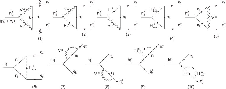
Figure 1: One-loop Feynman diagrams contributing to the decay $h^{0}_{1}\rightarrow e_{a}e_{b}$ in the unitary gauge. Here $V^{\pm}=W^{\pm},\,Y^{\pm}$.

The partial width of the decay is

$$\Gamma(h_{1}^{0}\rightarrow e_{a}e_{b})\equiv\Gamma(h_{1}^{0}\rightarrow e_{a}^{-}e_{b}^{+})+\Gamma(h^{0}_{1}\rightarrow e_{a}^{+}e_{b}^{-})=\frac{m_{h^{0}_{1}}}{8\pi}\left(|\Delta_{(ab)L}|^{2}+|\Delta_{(ab)R}|^{2}\right),$$ (60)

with the condition $m_{h_{1}^{0}}\gg m_{a,b}$. Where $m_{a,b}$ are the masses of muon and tau, respectively. The on-shell conditions for external particles are $p^{2}_{1,2}=m_{a,b}^{2}$ and $p_{h_{1}^{0}}^{2}\equiv(p_{1}+p_{2})^{2}=m^{2}_{h_{1}^{0}}$. The corresponding branching ratio is Br$(h^{0}_{1}\rightarrow e_{a}e_{b})=\Gamma(h_{1}^{0}\rightarrow e_{a}e_{b})/\Gamma^{\mathrm{total}}_{h_{1}^{0}},$ where $\Gamma^{\mathrm{total}}_{h_{1}^{0}}\simeq 4.1\times 10^{-3}$ GeV pdg2016 ; Gah01 . The $\Delta_{(ab)L,R}$ can be written as

$$\Delta_{(ab)L,R}=\sum_{i=1,5,7,8}\Delta^{(i)W}_{(ab)L,R}+\sum^{10}_{i=1}\Delta^{(i)Y}_{(ab)L,R},$$ (61)

where the analytic forms of $\Delta^{(i)W}_{(ab)L,R}$ and $\Delta^{(i)Y}_{(ab)L,R}$ are shown in the Appendix. They can be calculated using the unitary gauge with the same techniques given in Refs. issthhx ; HueNPB16 . We have crosschecked this with FORM form .

The divergence cancellation in the total amplitude (61) is proved analytically in the Appendix, based on the following strict equality:

$$U^{\nu}(\hat{M}^{\nu})^{2}U^{\nu\dagger} =(U^{\nu*}\hat{M}^{\nu}U^{\nu\dagger})^{*}U^{\nu*}\hat{M}^{\nu}U^{\nu\dagger}=M^{\nu*}M^{\nu}$$

$$=\begin{pmatrix}m_{D}^{*}m_{D}^{T}&0&m_{D}^{*}M_{R}\\ 0&m_{D}^{\dagger}m_{D}+M_{R}^{*}M_{R}^{T}&M^{*}_{R}\mu_{X}\\ M_{R}^{\dagger}m_{D}^{T}&\mu^{*}_{X}M_{R}^{T}&M^{\dagger}_{R}M_{R}+\mu_{X}^{*}\mu_{X}\end{pmatrix}$$ (62)

In the model under consideration, the divergent parts coming from the contributions of charged Higgs and heavy gauge bosons are related to both $(M^{\nu*}M^{\nu})_{(a+3)(b+3)}$ and $(M^{\nu*}M^{\nu})_{(a+6)(b+6)}$ ($a,b\leq 3$), which are affected by heavy neutrino masses. The cancellation in the total divergent part requires that the physical heavy neutrino masses and $U^{\nu}$ must be the exact values. Hence, approximate forms of the heavy neutrino masses and neutrino mixing matrix derived from the ISS mechanism cannot be applied. In contrast, we checked numerically that these formulas are safely used in the usual minimal ISS version extended directly from the SM, because the divergent parts are only involved with the elements $(M^{\nu*}M^{\nu})_{ab}=(m_{D}^{*}m_{D}^{T})_{(ab)}$.

Many of the contributions listed in Eq. (61) are suppressed, and hence they can be ignored in our numerical computation. From now on, we just focus on the decay $h^{0}_{1}\rightarrow\mu\tau$, and hence the simplified notations $\Delta_{L,R}\equiv\Delta_{(23)L,R}$ will be used. The decay $h^{0}_{1}\rightarrow\,e\tau$ has similar properties, so we do not need to discuss it more explicitly. We can see that $|\frac{\Delta_{L}}{\Delta_{R}}|\simeq\mathcal{O}\left(\frac{m_{\mu}}{m_{\tau}}\right)$. In addition, we prove in the Appendix that the following combinations are finite: $\Delta_{L,R}^{(1+5)W}$, $\Delta_{L,R}^{(7+8)W}$, $\Delta_{L,R}^{(4)YH_{2}}$, $\Delta_{L,R}^{(6+9+10)YH_{2}}$, $\Delta_{L,R}^{(4)YH_{1}}$, $\Delta_{L,R}^{(7+8)Y}$, and $(\Delta_{L,R}^{(1+2+3+5)Y}+\Delta_{L,R}^{(6+9+10)YH_{1}})$. With $m_{\mu,\tau}\ll m_{W}$, we have $B^{(1)}_{1}+B^{(2)}_{1},B^{(2)}_{1}-B^{(2)}_{0}\simeq 0$, and hence $\Delta_{L,R}^{(7+8)W},\Delta_{L,R}^{(7+8)Y}\simeq 0$. The two contributions $\Delta_{L,R}^{(4)YH^{\pm}_{1,2}}$ are also suppressed with a large $m_{H^{\pm}_{2}}$ for about a few TeV.

The four diagrams 4, 6, 9 and 10 in Fig. 1 include contributions from both charged Higgs bosons. They are not significantly affected by the $SU(3)_{L}$ scale $m_{Y}$, and thus they may enhance the partial decay widths of the LFVHDs if charged Higgs masses are small.

The regions of parameter space predicting large branching ratios for LFVHDs are affected strongly by the current experimental bound Br$(\mu\rightarrow e\gamma)<4.2\times 10^{-13}$ muega2016 . A very good approximate formula for this decay rate in the limit $m_{\mu},m_{e}\rightarrow 0$ is muega331

$$\mathrm{Br}(\mu\rightarrow e\gamma)=\frac{12\pi^{2}}{G_{F}^{2}}|D_{R}|^{2},$$ (63)

where $G_{F}=g^{2}/(4\sqrt{2}m_{W}^{2})$ and $D_{R}$ is the one-loop contribution from charged gauge and Higgs boson mediations, $D_{R}=D^{W}_{R}+D^{Y}_{R}+D^{H^{\pm}_{1}}_{R}+D^{H^{\pm}_{2}}_{R}$. The analytic forms are

$$D^{W}_{R} =-\frac{eg^{2}}{32\pi^{2}m_{W}^{2}}\sum_{i=1}^{9}U^{\nu*}_{ai}U^{\nu}_{bi}F(t_{iW}),$$

$$D^{Y}_{R} =-\frac{eg^{2}}{32\pi^{2}m_{Y}^{2}}\sum_{i=1}^{9}U^{\nu*}_{(a+3)i}U^{\nu}_{(b+3)i}F(t_{iY}),$$

$$D^{H^{\pm}_{k}}_{R} =-\frac{eg^{2}f_{k}}{16\pi^{2}m_{W}^{2}}\sum_{i=1}^{9}\left[\frac{\lambda^{L,k*}_{ai}\lambda^{L,k}_{bi}}{m^{2}_{H^{\pm}_{k}}}\times\frac{1-6t_{ik}+3t^{2}_{ik}+2t^{3}_{ik}-6t^{2}_{ik}\ln(t_{i_{k}})}{12(t_{ik}-1)^{4}}\right.$$

$$+\left.\frac{m_{n_{i}}\lambda^{L,k*}_{ai}\lambda^{\prime R,k}_{bi}}{m^{2}_{H^{\pm}_{k}}}\times\frac{-1+t_{ik}^{2}-2t_{ik}\ln(t_{ik})}{2(t_{ik}-1)^{3}}\right],$$ (64)

where

$$b =2,\;a=1,\;t_{iW}\equiv\frac{m^{2}_{n_{i}}}{m_{W}^{2}},\;t_{iY}\equiv\frac{m^{2}_{n_{i}}}{m_{Y}^{2}},\;t_{ik}\equiv\frac{m^{2}_{n_{i}}}{m^{2}_{H^{\pm}_{k}}},$$

$$f_{1} \equiv\frac{1}{2},\;f_{2}\equiv c^{2}_{\theta},\;\lambda^{\prime R,1}_{bi}\equiv U^{\nu}_{(b+3)i},\;\lambda^{\prime R,2}_{bi}\equiv U^{\nu}_{bi},$$

$$F(x) \equiv-\frac{10-43x+78x^{2}-49x^{3}+4x^{4}+18x^{3}\ln(x)}{12(x-1)^{4}}.$$ (65)

Because all charged Higgs bosons couple with heavy neutrinos through the Yukawa coupling matrix $h^{\nu}_{ab}$, this matrix is strongly affected by the upper bound $\mathcal{O}(10^{-13})$ on Br$(\mu\rightarrow e\gamma)$. In fact, our numerical investigation shows that the allowed regions with light charged Higgs masses are very narrow. The previous investigation in Ref. ISS331 showed that the 331ISS models predicts a large Br$(\mu\rightarrow e\gamma)$, where the allowed regions discussed there were chosen such that $k\sim\mathcal{O}(10^{3})$ and $M_{R}\leq 1$ TeV, implying that $z\sim\mathcal{O}(1)$ eV. We checked that our formulas are consistent with these results. In general, the allowed regions are very strict, and satisfy one of the following conditions. First, the regions have a small $z$ and large $|M_{R}|$ and $m_{H_{2}^{\pm}}$, implying $k\gg 1$, including those mainly discussed in Ref. ISS331 . Second, the regions allow for a large $m_{D}$ and small $k$, but the strong destructive correlation between the two-loop contributions of charged gauge and Higgs bosons must happen. These regions were also considered in Ref. ISS331 , but they were not given much attention. They are very interesting because they predict large branching ratios for LFVHDs and light particles such as new neutrinos and charged Higgs bosons, which could be found at the LHC and planned colliders Higg331 ; Heavynu . Hence, our numerical investigation will focus on this case.

IV Numerical discussion on LFVHDS

IV.1 Setup parameters

To numerically investigate the LFVHDs of the SM-like Higgs boson, we will use the following well-known experimental parameters pdg2016 : the mass of the $W$ boson $m_{W}=80.385$ GeV, the charged lepton masses $m_{e}=5\times 10^{-4}$ GeV, $m_{\mu}=0.105$ GeV, and $m_{\tau}=1.776$ GeV, the SM-like Higgs mass $m_{h^{0}_{1}}=125.1$ GeV, and the gauge coupling of the $SU(2)_{L}$ symmetry $g\simeq 0.651$.

Combined with the discussion in Sec. II, the independent parameters are the heavy neutrino mass scale $M_{R}=\mathrm{diag}(M_{R},\,M_{R},\,M_{R})$, the heavy gauge boson mass $m_{Y}$ considered as the $SU(3)_{L}$ breaking scale, the charged Higgs boson mass $m_{H^{\pm}_{2}}$, the characteristic scale of $m_{D}$ defined as the parameter $z$, and the two Higgs self-couplings $\lambda_{1,12}$.

Other parameters can be calculated in terms of the above free ones, namely,

$$v_{1} =v_{2}=\frac{\sqrt{2}m_{W}}{g},\;s_{\theta}=\frac{m_{W}}{m_{Y}\sqrt{2}},\;w=\frac{2m_{Y}}{g\,c_{\theta}},\;f=\frac{g\,c_{\theta}\,m^{2}_{H^{\pm}_{2}}}{4m_{Y}},\;m^{2}_{H^{\pm}_{1}}=\frac{m^{2}_{H^{\pm}_{2}}}{2}(t^{2}_{\theta}+1).$$ (66)

Apart from that, the mixing parameter $\alpha$ of the neutral CP-even Higgs was defined in Eq. (52). The Higgs self-coupling $\lambda_{2}$ is determined as HueNPB16

$$\lambda_{2}=\frac{t^{2}_{\theta}}{2}\left(\frac{m^{2}_{h^{0}_{1}}}{v_{1}}-\frac{m^{2}_{H^{\pm}_{2}}}{2w^{2}}\right)+\frac{\left(\lambda_{12}-\frac{m^{2}_{H^{\pm}_{2}}}{2w^{2}}\right)^{2}}{4\lambda_{1}-\frac{m^{2}_{h^{0}_{1}}}{v_{1}^{2}}}.$$ (67)

In the model under consideration with the quark sector given in Refs. chang ; Higg331 , only the charged Higgs bosons $H^{\pm}_{2}$ couple with all SM leptons and quarks. They have been investigated at the LHC in the direct production $pp\rightarrow t(b)H^{\pm}$, which then decay into two final fermion states cHiggs1 . But the specific constraints on them in the framework of the 3-3-1 models have not been mentioned yet, to the best of our knowledge. Instead, the lower bounds on their masses have been discussed recently based on recent data of neutral meson mixing $B_{0}-\bar{B}_{0}$, where a reasonable lower bound of $m_{H^{\pm}_{2}}\geq 480$ GeV was concerned Higg331 .

The values of $\lambda_{1,2,12}$ must satisfy theoretical conditions of unitarity and the Higgs potential must be bounded from below, as mentioned in Ref. HueNPB16 . The heavy charged gauge boson mass $m_{Y}$ is related to the recent lower constraint of neutral gauge boson $Z^{\prime}$ in this model.

For the above reasons, the default values of the free parameters chosen for our numerical investigation are as follows. Without loss of generality, the Higgs self-couplings are fixed as $\lambda_{1}=1,\,\lambda_{12}=-1$, which also guarantee that all couplings of the SM-like Higgs boson approach the SM limit when $t_{\theta}\rightarrow 0$. The default value $m_{Y}=4.5$ TeV satisfies all recent constraints Higg331 ; mYbound . The parameter $z$ will be considered in the range of the perturbative limit $z<2\sqrt{\pi}\times v_{1}\simeq 617$ GeV: in particular, we will fix $z=50,200,400$, $500$, and $600$ [GeV]. Finally, the charged Higgs mass $m_{H^{\pm}_{2}}$ will be investigated mainly in the range of $300$ to $5\times 10^{4}$ GeV, where large values of LFVHDs may appear.

IV.2 Numerical results

First, we reproduce the regions mentioned in Ref. ISS331 , where $M_{R}$ was chosen to be from hundreds of GeV to 1 TeV, and the scale of $m_{D}$ (namely, $z$), was a few GeV, corresponding to $k\gg 1$. As a result, the respective regions of parameter space always satisfy the experimental bound on Br$(\mu\rightarrow e\gamma)$ with large enough $m_{H^{\pm}_{2}}$. These regions are shown in Fig. 2 with fixed $z=1,5,10,100$, and $500$ GeV.

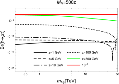
Figure 2: Br$(\mu\rightarrow e\gamma)$ (left) and Br$(h^{0}_{1}\rightarrow\mu\tau)$ (right) as functions of $m_{H^{\pm}_{2}}$ with $k=500$.

All allowed regions (i.e, those that satisfy the upper bound Br$(\mu\rightarrow e\gamma)<4.2\times 10^{-13}$) give a small Br$(h^{0}_{1}\rightarrow\mu\tau)<\mathcal{O}(10^{-9})$. In general, for larger $k$ we checked numerically that the values of the branching ratio of LFVHDs will decrease significantly, and hence we will not discuss this further.

With small values of $k=5.5$ and $9$, the dependence of both Br$(\mu\rightarrow e\gamma)$ and Br$(h\rightarrow\mu\tau)$ on $m_{H^{\pm}_{2}}$ with fixed $z$ are shown in Fig. 3.

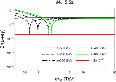
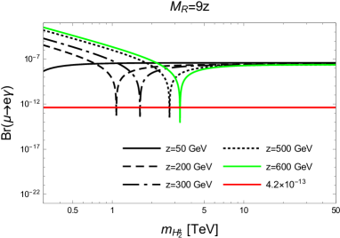
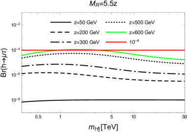
Figure 3: Br$(\mu\rightarrow e\gamma)$ (upper) and Br$(h^{0}_{1}\rightarrow\mu\tau)$ (lower) as functions of $m_{H^{\pm}_{2}}$ with $k=5.5$ (left) and $k=9$ (right).

Most regions of the parameter space are ruled out by the bound on Br$(\mu\rightarrow e\gamma)$, except for narrow parts where particular contributions from charged Higgs and gauge bosons are destructive. This interesting property of the 331ISS model was indicated previously in Ref. ISS331 . Furthermore, it predicts allowed regions that give a large Br$(h^{0}_{1}\rightarrow\mu\tau)$. In particular, the largest values can reach $\mathcal{O}(10^{-4})$ when $k=5.5$ and $z=600$ GeV, which is very close to the perturbative limit. In general, the illustrations in two Figs. 2 and 3 suggest that this branching ratio is enhanced significantly for smaller $k$ and larger $z$, but changes slowly with the change of large $m_{H^{\pm}_{2}}$. In contrast, small $m_{H^{\pm}_{2}}$ plays a very important role in creating allowed regions that predict a large LFVHD. Br$(\mu\rightarrow e\gamma)$ does not depend on $m_{H^{\pm}_{2}}$ when it is large enough. Furthermore, the branching ratio decreases with increasing $k$ and it will go below the experimental bound if $k$ is large enough.

The allowed regions in Fig. 3 are shown more explicitly in Fig. 4, corresponding to $k=5.5$ and $k=9$.

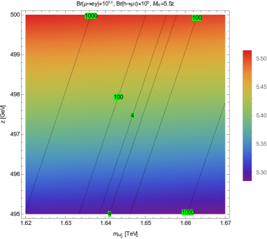
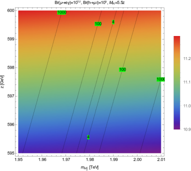
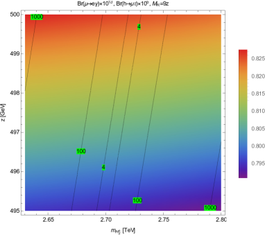
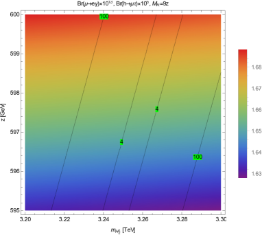
Figure 4: Density plots of Br$(h^{0}_{1}\rightarrow\mu\tau)$ and contour plots of Br$(\mu\rightarrow e\gamma)$ (black curves) as functions of $m_{H^{\pm}_{2}}$ and $z$, with $k=5.5$ (upper) and $k=9$ (lower).

Only regions that give a large Br$(h^{0}_{1}\rightarrow\mu\tau)$ are mentioned. They are bounded between two black curves representing the constant value of Br$(\mu\rightarrow e\gamma)\times 10^{13}=4$. Clearly, Br$(h^{0}_{1}\rightarrow\mu\tau)$ is sensitive to $z$ and $k$, while it changes slowly with changing values of $m_{H^{\pm}_{2}}$. In contrast, the suppressed Br$(\mu\rightarrow e\gamma)$ allows narrow regions of the parameter space, where some particular relation between $m_{H^{\pm}_{2}}$ and $k$ and $z$ is realized. Hence, if these two decay channel are discovered by experiments, depending on their specific values, a relation between heavy neutrino and charged Higgs masses can be determined from the 331ISS framework.

To understand how Br$(h^{0}_{1}\rightarrow\mu\tau)$ depends on the $SU(3)_{L}$ breaking scale defined by $m_{Y}$ in this work, four allowed regions corresponding to the four fixed values $m_{Y}=3,4,5$, and $6$ TeV are illustrated in Fig. 5.

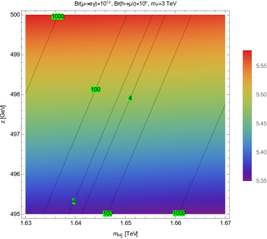
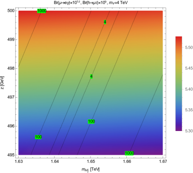
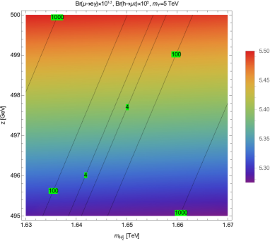
Figure 5: Density plots of Br$(h^{0}_{1}\rightarrow\mu\tau)$ and contour plots of Br$(\mu\rightarrow e\gamma)$ (black curves) as functions of $m_{H^{\pm}_{2}}$ and $z$, with $k=5.5$, $z$ around $500$ GeV and different $m_{Y}$.

It can be seen that the branching ratio of LFVHD depends weakly on $m_{Y}$, namely, it decreases slowly with increasing $m_{Y}$. Hence, studies of LFV decays will give useful information about heavy neutrinos and charged Higgs bosons besides the phenomenology arising from heavy gauge bosons discussed in many earlier works. More interestingly, this may happen at large $SU(3)_{L}$ scales which the LHC cannot detect at present.

V Conclusion

The 331ISS models seem to be the most interesting among the well-known 331 models because of their rich phenomenology, as indicated in many recent works. This work addressed a more attractive property, namely, the LFVHDs of the SM-like Higgs boson which are being investigated at the LHC. Assuming the absence of the tree-level decays $h^{0}_{1}\rightarrow e_{a}e_{b}$ and $e_{j}\rightarrow e_{i}\gamma$ ($j>i$), the analytical formulas at the one-loop level to calculate these decay rates in the 331ISS model have been introduced. The divergent cancellation in the total decay amplitudes of $h^{0}_{1}\rightarrow e_{a}e_{b}$ was shown explicitly. From the numerical investigation, we have indicated that the Br$(h^{0}_{1}\rightarrow\mu\tau)$ predicted by the 331ISS model can reach large values of $\mathcal{O}(10^{-5})$. They are even very close to $10^{-4}$, for example, in the special case with $k=5.5$ and $z\simeq 600$ GeV, which is close to the perturbative limit of the lepton Yukawa couplings. This value is larger than that predicted by the simplest ISS version extended directly from the SM issE . New charged Higgs bosons may give large contributions to both of the decay rates Br$(\mu\rightarrow e\gamma)$ and Br$(h^{0}_{1}\rightarrow\mu\tau)$, leading to either constructive or destructive correlations with those from the charged gauge bosons. As a by-product, the recent experimental bound on Br$(\mu\rightarrow e\gamma)$ rules out most of the regions of parameter space with small $k$ and large $z$, except the narrow regions arising from the destructive correlations between contributions of charged Higgs and gauge bosons. We have shown numerically that only these regions give large Br$(h^{0}_{1}\rightarrow\mu\tau)>10^{-5}$ when $\mathrm{400}$ GeV $\mathrm{<z<600}$ GeV and $k\leq 9$ in the case where the Majorana mass matrix $M_{R}$ is proportional to the identity one. Furthermore, these large values of Br$(h^{0}_{1}\rightarrow\mu\tau)$ depend weakly on the masses of the heavy charged gauge bosons, but they require the heavy neutrino mass scale $M_{R}$ and $m_{H^{\pm}_{2}}$ to be a few TeV, which can be detected at current colliders. Besides, Br$(h^{0}_{1}\rightarrow\tau e)$ has the same result. In conclusion, large branching ratios of the LFV processes like $h^{0}_{1}\rightarrow\mu\tau,e\tau$ will support the 331ISS model and may rule out the original 331RHN model containing only very light exotic neutrinos. Additionally, many properties of heavy neutrinos and charged Higgs bosons in the 331ISS framework may be determined independently at the $SU(3)_{L}$ scale.

Appendix A Form factors of LFVHDS in the unitary gauge

In this appendix we list all analytic formulas of one-loop contributions to LFVHDs defined in Eq. (61). They are written in terms of Passarino-Veltman functions that were defined thoroughly in Refs. HueNPB16 ; issthhx . Using the notations $D_{0}=k^{2}-M_{0}^{2}+i\delta$, $D_{1}=(k-p_{1})^{2}-M_{1}^{2}+i\delta$ and $D_{2}=(k+p_{2})^{2}-M_{2}^{2}+i\delta$, where $\delta$ is an infinitesimal a positive real quantity, the one-loop integrals and Passarino-Veltman functions needed in this work are

$$B^{(i)}_{0,\mu} \equiv \frac{\left(2\pi\mu\right)^{4-D}}{i\pi^{2}}\int\frac{d^{D}k\left\{1,k_{\mu}\right\}}{D_{0}D_{i}},\quad B^{(12)}_{0}\equiv\frac{\left(2\pi\mu\right)^{4-D}}{i\pi^{2}}\int\frac{d^{D}k}{D_{1}D_{2}},$$

$$C_{0,\mu} \equiv C_{0,\mu}(M_{0},M_{1},M_{2})=\frac{1}{i\pi^{2}}\int\frac{d^{4}k\left\{1,k_{\mu}\right\}}{D_{0}D_{1}D_{2}},$$

$$B^{(i)}_{\mu} = B^{(i)}_{1}p_{i\mu},\hskip 14.22636ptC_{\mu}=C_{1}p_{1\mu}+C_{2}p_{2\mu}$$

where $i=1,2$. In addition, $D=4-2\epsilon\leq 4$ is the dimension of the integral, $M_{0},~{}M_{1},~{}M_{2}$ are masses of virtual particles in the loop, and $\mu$ is an arbitrary mass parameter introduced via dimensional regularization DR . The external momenta of the final leptons shown in Fig. 1 satisfy $p^{2}_{1}=m^{2}_{a},~{}p^{2}_{2}=m^{2}_{b}$ and $(p_{1}+p_{2})^{2}=m^{2}_{h^{0}_{1}}$, where $m_{h^{0}_{1}}$ is the SM-like Higgs boson mass, and $m_{a,b}$ are lepton masses. In the limit $m_{a,b}\simeq 0$, the analytic formulas for $B^{(i)}_{0,1},\,B^{(12)}_{0},\,C_{0}$, and $C_{1,2}$ were shown in Refs. loop ; HueNPB16 ; issthhx , and hence we will not repeat them here. These functions are used for our numerical investigation. We stress that they were checked numerically to be well consistent with the exact results computed by LoopTooLS looptools , as reported in Ref. KhiemPTEP16 .

The analytic expressions for $\Delta^{(i)W}_{L,R}\equiv\Delta^{(i)W}_{(ab)L,R}$, where $i$ implies the diagram (i) in Fig. 1, are

$$\Delta^{(1)W}_{L} = \frac{g^{3}c_{\alpha}m_{a}}{64\pi^{2}m_{W}^{3}}\sum_{i=1}^{9}U^{\nu*}_{ai}U^{\nu}_{bi}\left\{m_{n_{i}}^{2}\left(B^{(1)}_{1}-B^{(1)}_{0}-B^{(2)}_{0}\right)-m_{b}^{2}B^{(2)}_{1}+\left(2m_{W}^{2}+m^{2}_{h^{0}_{1}}\right)m_{n_{i}}^{2}C_{0}\right.$$

$$- \left.\left[2m_{W}^{2}\left(2m_{W}^{2}+m_{n_{i}}^{2}+m_{a}^{2}-m_{b}^{2}\right)+m_{n_{i}}^{2}m_{h^{0}_{1}}^{2}\right]C_{1}+\left[2m_{W}^{2}\left(m_{a}^{2}-m^{2}_{h^{0}_{1}}\right)+m_{b}^{2}m^{2}_{h^{0}_{1}}\right]C_{2}\frac{}{}\right\},$$

$$\Delta^{(1)W}_{R} = \frac{g^{3}c_{\alpha}m_{b}}{64\pi^{2}m_{W}^{3}}\sum_{i=1}^{9}U^{\nu*}_{ai}U^{\nu}_{bi}\left\{-m_{n_{i}}^{2}\left(B^{(2)}_{1}+B^{(1)}_{0}+B^{(2)}_{0}\right)+m_{a}^{2}B^{(1)}_{1}+\left(2m_{W}^{2}+m^{2}_{h^{0}_{1}}\right)m_{n_{i}}^{2}C_{0}\right.$$

$$- \left.\left[2m_{W}^{2}\left(m_{b}^{2}-m^{2}_{h}\right)+m_{a}^{2}m^{2}_{h^{0}_{1}}\right]C_{1}+\left[2m_{W}^{2}\left(2m_{W}^{2}+m_{n_{i}}^{2}-m_{a}^{2}+m_{b}^{2}\right)+m_{n_{i}}^{2}m_{h^{0}_{1}}^{2}\right]C_{2}\frac{}{}\right\},$$

$$\Delta^{(5)W}_{L} = \frac{g^{3}c_{\alpha}m_{a}}{64\pi^{2}m_{W}^{3}}\sum_{i,j=1}^{9}U^{\nu*}_{ai}U^{\nu}_{bj}\left\{\lambda^{0*}_{ij}m_{n_{j}}\left[B^{(12)}_{0}-m_{W}^{2}C_{0}+\left(2m_{W}^{2}+m_{n_{i}}^{2}-m_{a}^{2}\right)C_{1}\right]\right.$$

$$\hskip 113.81102pt\left.+\lambda^{0}_{ij}m_{n_{i}}\left[B^{(1)}_{1}+\left(2m_{W}^{2}+m_{n_{j}}^{2}-m_{b}^{2}\right)C_{1}\right]\right\},$$

$$\Delta^{(5)W}_{R} = \frac{g^{3}c_{\alpha}m_{b}}{64\pi^{2}m_{W}^{3}}\sum_{i=1}^{9}U^{\nu*}_{ai}U^{\nu}_{bj}\left\{\lambda^{0}_{ij}m_{n_{i}}\left[B^{(12)}_{0}-m_{W}^{2}C_{0}-\left(2m_{W}^{2}+m_{n_{j}}^{2}-m_{b}^{2}\right)C_{2}\right]\right.$$

$$\hskip 105.2751pt-\left.\lambda^{0*}_{ij}m_{n_{j}}\left[B^{(2)}_{1}+\left(2m_{W}^{2}+m_{n_{i}}^{2}-m_{a}^{2}\right)C_{2}\right]\right\},$$

$$\Delta^{(7+8)W}_{L} = \frac{g^{3}m_{a}m_{b}^{2}c_{\alpha}}{64\pi^{2}m^{3}_{W}(m_{a}^{2}-m_{b}^{2})}\sum_{i=1}^{9}U^{\nu*}_{ai}U^{\nu}_{bi}\left[2m_{n_{i}}^{2}\left(B^{(1)}_{0}-B^{(2)}_{0}\right)\right.$$

$$- \left.\left(2m_{W}^{2}+m_{n_{i}}^{2}\right)\left(B^{(1)}_{1}+B^{(2)}_{1}\right)-m_{a}^{2}B^{(1)}_{1}-m_{b}^{2}B^{(1)}_{2}\right],$$

$$\Delta^{(7+8)W}_{R} = \frac{m_{a}}{m_{b}}\Delta^{(7+8)W}_{L}.$$ (68)

Defining $\Delta^{(i)Y}_{L,R}=\Delta^{(i)YH^{\pm}_{1}}_{(ab)L,R}+\Delta^{(i)YH^{\pm}_{2}}_{(ab)L,R}$ with $i=4,6,9,10$, the analytic expressions for $\Delta^{(i)Y}_{L,R}\equiv\Delta^{(i)Y}_{(ab)L,R}$ are

$$\Delta^{(1)Y}_{L} = -\frac{g^{3}m_{a}\left(\sqrt{2}s_{\alpha}c_{\theta}-c_{\alpha}s_{\theta}\right)}{64\sqrt{2}\pi^{2}m_{Y}^{3}}\sum_{i=1}^{9}U^{\nu*}_{(a+3)i}U^{\nu}_{(b+3)i}\left\{m_{n_{i}}^{2}\left(B^{(1)}_{1}-B^{(1)}_{0}-B^{(2)}_{0}\right)-m_{b}^{2}B^{(2)}_{1}\right.$$

$$+ \left.\left(2m_{Y}^{2}+m^{2}_{h^{0}_{1}}\right)m_{n_{i}}^{2}C_{0}-\left[2m_{Y}^{2}\left(2m_{Y}^{2}+m_{n_{i}}^{2}+m_{a}^{2}-m_{b}^{2}\right)+m_{n_{i}}^{2}m_{h^{0}_{1}}^{2}\right]C_{1}\right.$$

$$+ \left.\left[2m_{Y}^{2}\left(m_{a}^{2}-m^{2}_{h^{0}_{1}}\right)+m_{b}^{2}m^{2}_{h^{0}_{1}}\right]C_{2}\frac{}{}\right\},$$

$$\Delta^{(1)Y}_{R} = -\frac{g^{3}m_{b}\left(\sqrt{2}s_{\alpha}c_{\theta}-c_{\alpha}s_{\theta}\right)}{64\sqrt{2}\pi^{2}m_{Y}^{3}}\sum_{i=1}^{9}U^{\nu*}_{(a+3)i}U^{\nu}_{(b+3)i}\left\{-m_{n_{i}}^{2}\left(B^{(2)}_{1}+B^{(1)}_{0}+B^{(2)}_{0}\right)+m_{a}^{2}B^{(1)}_{1}\right.$$

$$+ \left.\left(2m_{Y}^{2}+m^{2}_{h^{0}_{1}}\right)m_{n_{i}}^{2}C_{0}-\left[2m_{Y}^{2}\left(m_{b}^{2}-m^{2}_{h^{0}_{1}}\right)+m_{a}^{2}m^{2}_{h^{0}_{1}}\right]C_{1}\right.$$

$$+ \left.\left[2m_{Y}^{2}\left(2m_{Y}^{2}+m_{n_{i}}^{2}-m_{a}^{2}+m_{b}^{2}\right)+m_{n_{i}}^{2}m_{h^{0}_{1}}^{2}\right]C_{2}\frac{}{}\right\},$$

$$\Delta^{(2)Y}_{L} = \frac{g^{3}m_{a}c_{\theta}\left(c_{\alpha}c_{\theta}+\sqrt{2}s_{\alpha}s_{\theta}\right)}{64\pi^{2}m_{W}m_{Y}^{2}}\sum_{i=1}^{9}U^{\nu*}_{(a+3)i}$$

$$\times \left\{\lambda^{L,1}_{bi}m_{n_{i}}\left[B^{(1)}_{0}-B^{(1)}_{1}+\left(m_{Y}^{2}+m_{H^{\pm}_{1}}^{2}-m_{h^{0}_{1}}^{2}\right)C_{0}+\left(m_{Y}^{2}-m_{H^{\pm}_{1}}^{2}+m_{h^{0}_{1}}^{2}\right)C_{1}\right]\right.$$

$$+\left.\lambda^{R,1}_{bi}m_{b}\left[2m_{Y}^{2}C_{1}-\left(m_{Y}^{2}+m_{H^{\pm}_{1}}^{2}-m_{h^{0}_{1}}^{2}\right)C_{2}\right]\right\},$$

$$\Delta^{(2)Y}_{R} = \frac{g^{3}c_{\theta}\left(c_{\alpha}c_{\theta}+\sqrt{2}s_{\alpha}s_{\theta}\right)}{64\pi^{2}m_{W}m_{Y}^{2}}\sum_{i=1}^{9}U^{\nu*}_{(a+3)i}$$

$$\times \left\{\lambda^{L,1}_{bi}m_{b}m_{n_{i}}\left[-2m_{Y}^{2}C_{0}-\left(m_{Y}^{2}-m_{H^{\pm}_{1}}^{2}+m_{h^{0}_{1}}^{2}\right)C_{2}\right]\right.$$

$$+\left.\lambda^{R,1}_{bi}\left[-m_{n_{i}}^{2}B^{(1)}_{0}+m_{a}^{2}B^{(1)}_{1}+m_{n_{i}}^{2}\left(m_{Y}^{2}-m_{H^{\pm}_{1}}^{2}+m_{h^{0}_{1}}^{2}\right)C_{0}\right.\right.$$

$$+\left.\left.\left[2m_{Y}^{2}\left(m_{h^{0}_{1}}^{2}-m_{b}^{2}\right)-m_{a}^{2}\left(m_{Y}^{2}-m_{H^{\pm}_{1}}^{2}+m_{h^{0}_{1}}^{2}\right)\right]C_{1}+2m_{b}^{2}m_{Y}^{2}C_{2}\right]\right\},$$

$$\Delta^{(3)Y}_{L} = \frac{g^{3}c_{\theta}\left(c_{\alpha}c_{\theta}+\sqrt{2}s_{\alpha}s_{\theta}\right)}{64\pi^{2}m_{W}m_{Y}^{2}}\sum_{i=1}^{9}U^{\nu}_{(b+3)i}$$

$$\times \left\{\lambda^{L,1*}_{ai}m_{a}m_{n_{i}}\left[-2m_{Y}^{2}C_{0}+\left(m_{Y}^{2}-m_{H^{\pm}_{1}}^{2}+m_{h^{0}_{1}}^{2}\right)C_{1}\right]\right.$$

$$+\left.\lambda^{R,1*}_{ai}\left[-m_{n_{i}}^{2}B^{(2)}_{0}-m_{b}^{2}B^{(2)}_{1}+m_{n_{i}}^{2}\left(m_{Y}^{2}-m_{H^{\pm}_{1}}^{2}+m_{h^{0}_{1}}^{2}\right)C_{0}\right.\right.$$

$$-\left.\left.2m_{a}^{2}m_{Y}^{2}C_{1}-\left[2m_{Y}^{2}\left(m_{h^{0}_{1}}^{2}-m_{a}^{2}\right)-m_{b}^{2}\left(m_{Y}^{2}-m_{H^{\pm}_{1}}^{2}+m_{h^{0}_{1}}^{2}\right)\right]C_{2}\right]\right\},$$

$$\Delta^{(3)Y}_{R} = \frac{g^{3}m_{b}c_{\theta}\left(c_{\alpha}c_{\theta}+\sqrt{2}s_{\alpha}s_{\theta}\right)}{64\pi^{2}m_{W}m_{Y}^{2}}\sum_{i=1}^{9}U^{\nu}_{(b+3)i}$$

$$\times \left\{\lambda^{L,1*}_{ai}m_{n_{i}}\left[B^{(2)}_{0}+B^{(2)}_{1}\right.\right.$$

$$\left.\left.+\left(m_{Y}^{2}+m_{H^{\pm}_{1}}^{2}-m_{h^{0}_{1}}^{2}\right)C_{0}-\left(m_{Y}^{2}-m_{H^{\pm}_{1}}^{2}+m_{h^{0}_{1}}^{2}\right)C_{2}\right]\right.$$

$$+\left.\lambda^{R,1*}_{ai}m_{a}\left[\left(m_{Y}^{2}+m_{H^{\pm}_{1}}^{2}-m_{h^{0}_{1}}^{2}\right)C_{1}-2m_{Y}^{2}C_{2}\right]\right\},$$

$$\Delta^{(4)YH^{\pm}_{k}}_{L} = \frac{g^{2}\lambda^{\pm}_{H_{k}}f_{k}}{16\pi^{2}m_{W}^{2}}\sum_{i=1}^{9}\left[-\lambda^{R,k*}_{ai}\lambda^{L,k}_{bi}m_{n_{i}}C_{0}-\lambda^{L,k*}_{ai}\lambda^{L,k}_{bi}m_{a}C_{1}+\lambda^{R,k*}_{ai}\lambda^{R,k}_{bi}m_{b}C_{2}\right],$$

$$\Delta^{(4)YH^{\pm}_{k}}_{R} = \frac{g^{2}\lambda^{\pm}_{H_{k}}f_{k}}{16\pi^{2}m_{W}^{2}}\sum_{i=1}^{9}\left[-\lambda^{L,k*}_{ai}\lambda^{R,k}_{bi}m_{n_{i}}C_{0}-\lambda^{R,k*}_{ai}\lambda^{R,k}_{bi}m_{a}C_{1}+\lambda^{L,k*}_{ai}\lambda^{L,k}_{bi}m_{b}C_{2}\right],$$

$$\Delta^{(5)Y}_{L} = \frac{g^{3}c_{\alpha}m_{a}}{64\pi^{2}m_{W}m_{Y}^{2}}$$

$$\times \sum_{i,j=1}^{9}U^{\nu*}_{(a+3)i}U^{\nu}_{(b+3)j}\left\{\lambda^{0*}_{ij}m_{n_{j}}\left[B^{(12)}_{0}-m_{Y}^{2}C_{0}+\left(2m_{Y}^{2}+m_{n_{i}}^{2}-m_{a}^{2}\right)C_{1}\right]\right.$$

$$\hskip 99.58464pt+\left.\lambda^{0}_{ij}m_{n_{i}}\left[B^{(1)}_{1}+\left(2m_{Y}^{2}+m_{n_{j}}^{2}-m_{b}^{2}\right)C_{1}\right]\right\},$$

$$\Delta^{(5)Y}_{R} = \frac{g^{3}c_{\alpha}m_{b}}{64\pi^{2}m_{W}m_{Y}^{2}}$$

$$\times \sum_{i,j=1}^{9}U^{\nu*}_{(a+3)i}U^{\nu}_{(b+3)j}\left\{\lambda^{0}_{ij}m_{n_{i}}\left[B^{(12)}_{0}-m_{Y}^{2}C_{0}-\left(2m_{Y}^{2}+m_{n_{j}}^{2}-m_{b}^{2}\right)C_{2}\right]\right.$$

$$\hskip 85.35826pt-\left.\lambda^{0*}_{ij}m_{n_{j}}\left[B^{(2)}_{1}+\left(2m_{Y}^{2}+m_{n_{i}}^{2}-m_{a}^{2}\right)C_{2}\right]\right\},$$

$$\Delta^{(6)YH^{\pm}_{k}}_{L} = -\frac{g^{3}c_{\alpha}f_{k}}{32\pi^{2}m_{W}^{3}}\sum_{i,j=1}^{9}\left\{\lambda^{0*}_{ij}\left[\lambda^{R,k*}_{ai}\lambda^{L,k}_{bj}\left(B^{(12)}_{0}+m_{H^{\pm}_{k}}^{2}C_{0}-m_{a}^{2}C_{1}+m_{b}^{2}C_{2}\right)\right.\right.$$

$$+ \left.\left.\lambda^{R,k*}_{ai}\lambda^{R,k}_{bj}m_{b}m_{n_{j}}C_{2}-\lambda^{L,k*}_{ai}\lambda^{L,k}_{bj}m_{a}m_{n_{i}}C_{1}\right]\right.$$

$$+ \left.\lambda^{0}_{ij}\left[\lambda^{R,k*}_{ai}\lambda^{L,k}_{bj}m_{n_{i}}m_{n_{j}}C_{0}+\lambda^{R,k*}_{ai}\lambda^{R,k}_{bj}m_{n_{i}}m_{b}(C_{0}+C_{2})\right.\right.$$

$$+ \left.\left.\lambda^{L,k*}_{ai}\lambda^{L,k}_{bj}m_{a}m_{n_{j}}(C_{0}-C_{1})+\lambda^{L,k*}_{ai}\lambda^{R,k}_{bj}m_{a}m_{b}(C_{0}-C_{1}+C_{2})\right]\frac{}{}\right\},$$

$$\Delta^{(6)YH^{\pm}_{k}}_{R} = -\frac{g^{3}c_{\alpha}f_{k}}{32\pi^{2}m_{W}^{3}}\sum_{i,j=1}^{9}\left\{\lambda^{0}_{ij}\left[\lambda^{L,k*}_{ai}\lambda^{R,k}_{bj}\left(B^{(12)}_{0}+m_{H^{\pm}_{k}}^{2}C_{0}-m_{a}^{2}C_{1}+m_{b}^{2}C_{2}\right)\right.\right.$$

$$+ \left.\left.\lambda^{L,k*}_{ai}\lambda^{L,k}_{bj}m_{b}m_{n_{j}}C_{2}-\lambda^{R,k*}_{ai}\lambda^{R,k}_{bj}m_{a}m_{n_{i}}C_{1}\right]\right.$$

$$+ \left.\lambda^{0*}_{ij}\left[\lambda^{L,k*}_{ai}\lambda^{R,k}_{bj}m_{n_{i}}m_{n_{j}}C_{0}+\lambda^{L,k*}_{ai}\lambda^{L,k}_{bj}m_{n_{i}}m_{b}(C_{0}+C_{2})\right.\right.$$

$$+ \left.\left.\lambda^{R,k*}_{ai}\lambda^{R,k}_{bj}m_{a}m_{n_{j}}(C_{0}-C_{1})+\lambda^{R,k*}_{ai}\lambda^{L,k}_{bj}m_{a}m_{b}(C_{0}-C_{1}+C_{2})\right]\frac{}{}\right\},$$

$$\Delta^{(7+8)Y}_{L} = \frac{g^{3}m_{a}m_{b}^{2}c_{\alpha}}{64\pi^{2}m_{W}m_{Y}^{2}(m_{a}^{2}-m_{b}^{2})}\sum_{i=1}^{9}U^{\nu*}_{(a+3)i}U^{\nu}_{(b+3)i}$$

$$\times \left[2m_{n_{i}}^{2}\left(B^{(1)}_{0}-B^{(2)}_{0}\right)-\left(2m_{Y}^{2}+m_{n_{i}}^{2}\right)\left(B^{(1)}_{1}+B^{(2)}_{1}\right)-m_{a}^{2}B^{(1)}_{1}-m_{b}^{2}B^{(2)}_{1}\right],$$

$$\Delta^{(7+8)Y}_{R} = \frac{m_{a}}{m_{b}}\Delta^{(7+8)Y}_{L},$$

$$\Delta^{(9+10)YH^{\pm}_{k}}_{L} = -\frac{g^{3}c_{\alpha}f_{k}}{32\pi^{2}m_{W}^{3}\left(m_{a}^{2}-m_{b}^{2}\right)}$$

$$\times \sum_{i=1}^{9}\left[m_{a}m_{b}m_{n_{i}}\lambda^{L,k*}_{ai}\lambda^{R,k}_{bi}\left(B^{(1)}_{0}-B^{(2)}_{0}\right)+m_{n_{i}}\lambda^{R,k*}_{ai}\lambda^{L,k}_{bi}\left(m^{2}_{b}B^{(1)}_{0}-m^{2}_{a}B^{(2)}_{0}\right)\right.$$

$$\left.+m_{a}m_{b}\left(\lambda^{L,k*}_{ai}\lambda^{L,k}_{bi}m_{b}+\lambda^{R,k*}_{ai}\lambda^{R,k}_{bi}m_{a}\right)\left(B^{(1)}_{1}+B^{(2)}_{1}\right)\right],$$

$$\Delta^{(9+10)YH^{\pm}_{k}}_{R} = -\frac{g^{3}c_{\alpha}f_{k}}{32\pi^{2}m_{W}^{3}\left(m_{a}^{2}-m_{b}^{2}\right)}$$ (69)

$$\times \sum_{i=1}^{9}\left[m_{a}m_{b}m_{n_{i}}\lambda^{R,k*}_{ai}\lambda^{L,k}_{bi}\left(B^{(1)}_{0}-B^{(2)}_{0}\right)+m_{n_{i}}\lambda^{L,k*}_{ai}\lambda^{R,k}_{bi}\left(m^{2}_{b}B^{(1)}_{0}-m^{2}_{a}B^{(2)}_{0}\right)\right.$$

$$\left.+m_{a}m_{b}\left(\lambda^{R,k*}_{ai}\lambda^{R,k}_{bi}m_{b}+\lambda^{L,k*}_{ai}\lambda^{L,k}_{bi}m_{a}\right)\left(B^{(1)}_{1}+B^{(2)}_{1}\right)\right],$$

where $f_{1}=c^{2}_{\theta}$ and $f_{2}=1/2$. The details to derive the expressions in Eq. (69) are the same as those shown in Refs. issthhx ; HueNPB16 , and hence we do not present them in this work. We note that the scalar functions $\Delta^{(1)W}_{L,R}$ and $\Delta^{(1,2,3)Y}_{L,R}$ include parts that do not depend on $m_{n_{i}}$, and therefore they vanish because of the Glashow-Iliopoulos-Maiani mechanism. They are ignored in Eqs. (68) and (69).

The divergent cancellation in the total $\Delta_{L,R}$ is shown as follows. The divergent parts only contain $B$ functions: div$B^{(1)}_{0}=$div$B^{(2)}_{0}=$div$B^{(12)}_{0}=2$div$B^{(1)}_{1}=-2$ div$B^{(2)}_{1}=\Delta_{\epsilon}$. Ignoring the common factor of $g^{3}/(64\pi^{2}m_{W}^{3})$ and using $1/m_{Y}=\sqrt{2}s_{\theta}/m_{W}$, the divergent parts of $\Delta_{L}$ derived from Eq. (69) are

$$\mathrm{div}\left[\Delta^{(1)W}_{L}\right] = m_{a}\Delta_{\epsilon}\times\left(-\frac{3c_{\alpha}}{2}\right)\sum_{i=1}^{9}U^{\nu*}_{ai}U^{\nu}_{bi}m^{2}_{n_{i}},$$

$$\mathrm{div}\left[\Delta^{(5)W}_{L}\right] = m_{a}\Delta_{\epsilon}\times c_{\alpha}\sum_{i,j=1}^{9}U^{\nu*}_{ai}U^{\nu}_{bj}\left(\lambda^{0*}_{ij}m_{n_{j}}+\frac{1}{2}\lambda^{0}_{ij}m_{n_{i}}\right),$$

$$\mathrm{div}\left[\Delta^{(7+8)W}_{L}\right] = \mathrm{div}\left[\Delta^{(4)Y}_{L}\right]=\mathrm{div}\left[\Delta^{(7+8)Y}_{L}\right]=0,$$

$$\mathrm{div}\left[\Delta^{(1)Y}_{L}\right] = m_{a}\Delta_{\epsilon}\times 3s_{\theta}^{3}\left(\sqrt{2}s_{\alpha}c_{\theta}-c_{\alpha}s_{\theta}\right)\sum_{i=1}^{9}U^{\nu*}_{(a+3)i}U^{\nu}_{(b+3)i}m^{2}_{n_{i}},$$

$$\mathrm{div}\left[\Delta^{(2)Y}_{L}\right] = m_{a}\Delta_{\epsilon}\times s_{\theta}^{2}c_{\theta}\left(c_{\alpha}c_{\theta}+\sqrt{2}s_{\alpha}s_{\theta}\right)\sum_{i=1}^{9}U^{\nu*}_{(a+3)i}\lambda^{L,1}_{bi}m_{n_{i}},$$

$$\mathrm{div}\left[\Delta^{(3)Y}_{L}\right] = m_{a}\Delta_{\epsilon}\times\left[-2s_{\theta}^{2}c_{\theta}\left(c_{\alpha}c_{\theta}+\sqrt{2}s_{\alpha}s_{\theta}\right)\right]\sum_{i=1}^{9}U^{\nu*}_{(a+3)i}U^{\nu}_{(b+3)i}m^{2}_{n_{i}},$$

$$\mathrm{div}\left[\Delta^{(5)Y}_{L}\right] = m_{a}\Delta_{\epsilon}\times 2s_{\theta}^{2}c_{\alpha}\sum_{i,j=1}^{9}U^{\nu*}_{(a+3)i}U^{\nu}_{(b+3)j}\left(\lambda^{0*}_{ij}m_{n_{j}}+\frac{1}{2}\lambda^{0}_{ij}m_{n_{i}}\right),$$

$$\mathrm{div}\left[\Delta^{(6)YH_{1}^{\pm}}_{L}\right] = m_{a}\Delta_{\epsilon}\times\left(-2c_{\alpha}c_{\theta}^{2}\right)\sum_{i,j=1}^{9}U^{\nu*}_{(a+3)i}\lambda^{0*}_{ij}\lambda^{L,1}_{bj},$$

$$\mathrm{div}\left[\Delta^{(6)YH_{2}^{\pm}}_{L}\right] = m_{a}\Delta_{\epsilon}\times\left(-c_{\alpha}\right)\sum_{i,j=1}^{9}U^{\nu*}_{ai}\lambda^{0*}_{ij}\lambda^{L,2}_{bj},$$

$$\mathrm{div}\left[\Delta^{(9+10)YH_{1}^{\pm}}_{L}\right] = m_{a}\Delta_{\epsilon}\times\left(2c_{\alpha}c_{\theta}^{2}\right)\sum_{i=1}^{9}U^{\nu*}_{(a+3)i}\lambda^{L,1}_{bi}m_{n_{i}},$$

$$\mathrm{div}\left[\Delta^{(9+10)YH_{2}^{\pm}}_{L}\right] = m_{a}\Delta_{\epsilon}\times c_{\alpha}\sum_{i=1}^{9}U^{\nu*}_{ai}\lambda^{L,2}_{bi}m_{n_{i}},$$ (70)

Using the equalities $M^{\nu}=U^{\nu*}\hat{M^{\nu}}U^{\nu\dagger}$ and Eq. (III.2), we can prove that

$$\mathrm{div}\left[\Delta^{(1)W}_{L,R}\right] \sim \sum_{i=1}^{9}U^{\nu*}_{ai}U^{\nu}_{bi}m^{2}_{n_{i}}=\left[U^{\nu}(\hat{M}^{\nu})^{2}U^{\nu\dagger}\right]_{ba}=(m_{D}^{*}m_{D}^{T})_{ba}$$

$$= (m_{D}^{\dagger}m_{D})_{ba},$$

$$\mathrm{div}\left[\Delta^{(5)W}_{L,R}\right] \sim \sum_{i,j=1}^{9}U^{\nu*}_{ai}U^{\nu}_{bj}\lambda^{0*}_{ij}m_{n_{j}},\,\sum_{i,j=1}^{9}U^{\nu*}_{ai}U^{\nu}_{bj}\lambda^{0}_{ij}m_{n_{i}}=(m_{D}^{*}m_{D}^{T})_{ba}$$

$$= (m_{D}^{\dagger}m_{D})_{ba},$$

$$\mathrm{div}\left[\Delta^{(1,3)Y}_{L,R}\right] \sim \sum_{i=1}^{9}U^{\nu*}_{(a+3)i}U^{\nu}_{(b+3)i}m^{2}_{n_{i}}=\left[U^{\nu}(\hat{M}^{\nu})^{2}U^{\nu\dagger}\right]_{(b+3)(a+3)}$$

$$= (m_{D}^{\dagger}m_{D}+M_{R}^{*}M_{R}^{T})_{ba},$$

$$\mathrm{div}\left[\Delta^{(2)Y,\,(9+10)YH^{\pm}_{1}}_{L,R}\right] \sim \sum_{i=1}^{9}U^{\nu*}_{(a+3)i}\lambda^{L,1}_{bi}m_{n_{i}}=(m_{D}^{*}m_{D})_{ba}+t^{2}_{\theta}(M^{*}_{R}M^{T}_{R})_{ba}$$

$$= -(m_{D}^{\dagger}m_{D})_{ba}+t^{2}_{\theta}(M^{*}_{R}M^{T}_{R})_{ba},$$

$$\mathrm{div}\left[\Delta^{(5)Y}_{L,R}\right] \sim \sum_{i,j=1}^{9}U^{\nu*}_{(a+3)i}U^{\nu}_{(b+3)j}\lambda^{0*}_{ij}m_{n_{j}},\,\sum_{i,j=1}^{9}U^{\nu*}_{(a+3)i}U^{\nu}_{(b+3)j}\lambda^{0}_{ij}m_{n_{i}}$$

$$\sim (m_{D}^{\dagger}m_{D})_{ba}-\sqrt{2}t_{\alpha}t_{\theta}(M^{*}_{R}M^{T}_{R})_{ba},$$

$$\mathrm{div}\left[\Delta^{(6)YH^{\pm}_{1}}_{L,R}\right] \sim \sum_{i,j=1}^{9}U^{\nu*}_{(a+3)i}\lambda^{0*}_{ij}\lambda^{L,1}_{bj}=(m_{D}^{*}m_{D})_{ba}-\sqrt{2}t_{\alpha}t_{\theta}^{3}(M^{*}_{R}M^{T}_{R})_{ba}$$

$$= -(m_{D}^{\dagger}m_{D})_{ba}-\sqrt{2}t_{\alpha}t_{\theta}^{3}(M^{*}_{R}M^{T}_{R})_{ba},$$

$$\mathrm{div}\left[\Delta^{(6)YH^{\pm}_{2}}_{L,R}\right] \sim \sum_{i,j=1}^{9}U^{\nu*}_{ai}\lambda^{0*}_{ij}\lambda^{L,2}_{bj}=-(m_{D}^{\dagger}m_{D})_{ba},$$

$$\mathrm{div}\left[\Delta^{(9+10)YH^{\pm}_{2}}_{L,R}\right] \sim \sum_{i=1}^{9}U^{\nu*}_{ai}\lambda^{L,2}_{bi}m_{n_{i}}=-(m_{D}^{\dagger}m_{D})_{ba},$$ (71)

where we have used the antisymmetric property of $m_{D}$: $m_{D}^{T}=-m_{D}$. From this, it can be seen that $\mathrm{div}\left[\Delta^{(1)W}_{L}\right]+\mathrm{div}\left[\Delta^{(5)W}_{L}\right]=\mathrm{div}\left[\Delta^{(6)YH^{\pm}_{2}}_{L}\right]+\mathrm{div}\left[\Delta^{(9+10)YH^{\pm}_{2}}_{L}\right]=0$. The sum of the remaining divergent parts is

$$\mathrm{div}\left[\Delta^{(1+2+3+5)Y}_{L}+\Delta^{(6+9+10)YH^{\pm}_{1}}_{L}\right]$$

$$\sim(m_{D}^{\dagger}m_{D})_{ba}\left\{\sqrt{2}s_{\alpha}s^{2}_{\theta}c_{\theta}(3-1-2)+c_{\alpha}\left[s^{2}_{\theta}(-3s^{2}_{\theta}-c^{2}_{\theta}-2c^{2}_{\theta}+3)+2s^{2}_{\theta}-2s^{2}_{\theta}\right]\right\}$$

$$+(M^{*}_{R}M^{T}_{R})_{ba}\left[\sqrt{2}s_{\alpha}\frac{s^{2}_{\theta}}{c_{\theta}}\left(3c^{2}_{\theta}+s^{2}_{\theta}-2c^{2}_{\theta}-3+2\right)+c_{\alpha}s^{2}_{\theta}\left(-3s^{2}_{\theta}+s^{2}_{\theta}-2c^{2}_{\theta}+2\right)\right]$$

$$=0.$$ (72)

Finally, the proof of the divergent cancellation in $\Delta_{R}$ is exactly the same as that in $\Delta_{L}$.

References

- (1) CMS Collaboration, Phys.Lett. B 749, 337 (2015); Phys. Lett. B 763, 472 (2016); ATLAS Collaboration, JHEP 1511, 211 (2015); Eur. Phys. J. C 77, 70 (2017); CMS Collaboration, ”Search for lepton flavour violating decays of the Higgs boson to and in proton-proton collisions at TeV”, arXiv:1712.07173.
- (2) ATLAS Collaboration, Phys. Lett. B 716, 1 (2012); CMS Collaboration, Phys. Lett. B 716, 30 (2012); CMS Collaboration, JHEP 1306, 081 (2013).
- (3) S. Kanemura, K. Matsuda, T. Ota, T. Shindou, E. Takasugi and K.Tsumura, Phys. Lett. B 599, 83 (2004); S. Davidson and P. Verdier, Phys. Rev. D 86, 111701 (2012); S. Bressler, A. Dery, and A. Efrati, Phys. Rev. D 90, 015025 (2014); D. A. Sierra and A. Vicente, Phys. Rev. D 90, 115004 (2014); C. X. Yue, C. Pang, and Y. C. Guo, J. Phys. G 42, 075003 (2015); S. Banerjee, B. Bhattacherjee, M. Mitra, and M. Spannowsky, JHEP 1607, 059 (2016); I. Chakraborty, A. Datta, and A. Kundu, J.Phys. G 43, 125001 (2016); Q. Qin, Q. Li, C.D. Lu, F.S.Yu, and S.H. Zhou, Charged lepton flavor violating Higgs decays at the CEPC, arXiv:1711.07243.
- (4) G. Blankenburg, J. Ellis, and G. Isidori, Phys. Lett. B 712, 386 (2012); J. H. Garcia, N. Rius, and A. Santamaria, JHEP 1611, 084 (2016).
- (5) A. Pilaftsis, Phys.Lett. B 285, 68 (1992); A. Pilaftsis, Z.Phys. C 55, 275 (1992); J. G. Korner, A. Pilaftsis, and K. Schilcher, Phys. Rev. D 47, 1080 (1993); A. Ilakovac, Phys.Rev. D 62, 036010 (2000); J.L. Diaz-Cruz, and J.J. Toscano, Phys.Rev. D 62, 116005 (2000); A. Goudelis, O. Lebedev, and J.H. Park, Phys.Lett. B 707, 369 (2012); P.S. Bhupal Dev, R. Franceschini, and R.N. Mohapatra, Phys.Rev. D 86, 093010 (2012); R. Harnik, J. Kopp, and J. Zupan, JHEP 1303, 026 (2013); A. Falkowski, D. M. Straub, and A. Vicente, JHEP 1405, 092 (2014); A. Celis, V. Cirigliano, and E. Passemar, Phys. Rev. D 89, 013008 (2014); A. Dery, A. Efrati, Y. Nir, Y. Soreq, and V. Susi, Phys. Rev. D 90, 115022 (2014); X. G. He, J.Tandean, and Y. J. Zheng, JHEP 1509, 093 (2015); I. Dorsner, S. Fajfer, A. Greljo, J. F. Kamenik, N. Kosnik, and Ivan Nisandzic, JHEP 1506, 108 (2015); J. Heeck, M. Holthausen, W. Rodejohann, and Y. Shimizu, Nucl. Phys. B896, 281 (2015); A. Crivellin, G. DAmbrosio, and J. Heeck, Phys. Rev. D 91, 075006 (2015); L. D . Lima, C. S. Machado, R. D. Matheus, and L. A. F. D. Prado, JHEP 1511, 074 (2015); I. D. M. Varzielas, O. Fischer, and V. Maurer, JHEP 1508, 080 (2015); Y. Omura, E. Senaha, and K. Tobe, JHEP 1505, 028 (2015); M. D. Campos, A. E. C. Hernández, H. Päs, and E. Schumacher, Phys.Rev. D 91, 116011 (2015); A. Crivellin, G. D’Ambrosio, and J. Heeck, Phys. Rev. Lett. 114, 151801 (2015); D. Das and A. Kundu, Phys.Rev. D 92, 015009 (2015); A. Lami, and P. Roig, Phys.Rev. D 94, 056001 (2016); Y. Omura, E. Senaha, and K. Tobe, Phys. Rev. D 94, 055019 (2016); W. Altmannshofer, S. Gori, A. L. Kagan, L. Silvestrini, and J. Zupan, Phys. Rev. D 93, 031301 (2016); C. F. Chang, C. H. V. Chang, C. S. Nugroho, and T. C. Yuan, Nucl.Phys. B910, 293 (2016); C. H. Chen, and T. Nomura, Eur.Phys.J. C 76, 353 (2016); K. Huitu, V. Keus, N. Koivunen, and O. Lebedev, JHEP 1605, 026 (2016); K. Cheung, W. Y. Keung, and P. Y. Tseng, Phys. Rev. D 93, 015010 (2016); N. Bizot, S. Davidson, M. Frigerio, and J. L. Kneur, JHEP 1603, 073 (2016); M. Sher, and K. Thrasher, Phys. Rev. D 93, 055021 (2016); M. Aoki, S. Kanemura, K. Sakurai, and H. Sugiyama, Phys.Lett. B 763, 352 (2016); H.K. Guo, Y.Y. Li, T. Liu, M. R. Musolf, and J. Shu, Phys.Rev. D 96, 115034 (2017); J. H. Garcia, T. Ohlsson, S. Riad, and J. Wiren, JHEP 1704, 130 (2017); B. Yang, J. Han, and N. Liu, Phys.Rev. D 95, 035010 (2017).
- (6) L.T. Hue, H.N. Long, T.T. Thuc, and T. Phong Nguyen, Nucl.Phys. B907, 37 (2016); T.T. Thuc, L.T. Hue, H.N. Long, and T. Phong Nguyen, Phys.Rev. D 93, 115026 (2016).
- (7) A. Brignole, and A. Rossi, Phys. Lett. B 566, 217 (2003) 036; J. L. Diaz-Cruz, JHEP 0305, 036 (2003); A. Brignole, and A. Rossi, Nucl. Phys. B701, 3 (2004); E. Arganda, A. M. Curiel, M. J. Herrero, and D. Temes, Phys.Rev. D 71, 035011 (2005); P. T. Giang, L. T. Hue, D. T. Huong, and H. N. Long, Nucl. Phys. B864, 85 (2012); M. A, Catania, E. Arganda, and M. J. Herrero, JHEP 1309, 160 (2013); D. T. Binh, L. T. Hue, D. T. Huong, and H. N. Long, Eur. Phys. J. C 74, 2851 (2014); M. A. Catania, E. Arganda, and M. J. Herrero, JHEP 1510, 192 (2015); E. Arganda, M. J. Herrero, R. Morales, and A. Szynkman, JHEP 1603, 055 (2016); E. Arganda, M. J. Herrero, X. Marcano, and C. Weiland, Phys. Rev. D 93, 055010 (2016); S. Baek, and Z.F. Kang, JHEP 1603, 106 (2016); S. Baek, and K. Nishiwaki, Phys. Rev. D 93, 015002 (2016); H.B. Zhang, T.F. Feng, S.M. Zhao, and Y.L. Yan, Chin.Phys. C 41, 043106 (2017).
- (8) S. M. Boucenna, J. W. F. Valle, and A. Vicente, Phys.Rev. D 92, 053001 (2015).
- (9) G. Arcadi, C.P. Ferreira, F. Goertz, M.M. Guzzo, F. S. Queiroz, A.C.O. Santos, Lepton Flavor Violation Induced by Dark Matter, arXiv:1712.02373 [Phys.Rev.D (to be published)].
- (10) M. Lindner, M. Platscher, and F. S. Queiroz, Phys.Rep. 731, 1 (2018).
- (11) L.T. Hue, L.D. Ninh, T.T. Thuc, and N.T.T. Dat, Eur.Phys.J. C 78, 128 (2018).
- (12) F. Pisano, V. Pleitez, Phys. Rev. D 46, 410 (1992); P. H. Frampton, Phys. Rev. Lett. 69, 2889 (1992).
- (13) M. Singer, J.W. F. Valle, and J. Schechter, Phys. Rev. D 22, 738 (1980); R. Foot, H. N. Long, and Tuan A. Tran, Phys. Rev. D 50, R34 (1994); J. C. Montero, F. Pisano, and V. Pleitez, Phys. Rev. D 47, 2918 (1993); H. N. Long, Phys. Rev. D 53, 437 (1996); D 54, 4691 (1996).
- (14) J. K. Mizukoshi, C. A. de S. Pires, and F. S. Queiroz, and P. S. Rodrigues da Silva, Phys. Rev. D 83, 065024 (2011); Alex G. Dias, C. A. de S. Pires, and P. S. Rodrigues da Silva, Phys.Lett. B 628, 85 (2005).
- (15) M.E. Catano, R Martinez, and F. Ochoa, Phys.Rev. D 86, 073015 (2012); A. G. Dias, C. A. de S.Pires, P. S. Rodrigues da Silva, and A. Sampieri, Phys.Rev. D 86, 035007 (2012).
- (16) D. Chang, and H.N. Long, Phys.Rev. D 73, 053006 (2006).
- (17) E. Arganda, M. J. Herrero, X. Marcano, and C. Weiland, Phys.Rev. D 91, 015001 (2015); E. Arganda, M.J. Herrero, X. Marcano, R. Morales, and A. Szynkman, Phys.Rev. D 95, 095029 (2017).
- (18) A.J. Buras, F. D. Fazio, J. Girrbach, and M.V. Carlucci, JHEP 1302 (2013) 023.
- (19) L.T. Hue, and L.D. Ninh, Mod.Phys.Lett. A 31, 1650062 (2016).
- (20) M. B. Tully and G. C. Joshi, Phys. Rev. D 64, 011301(R) (2001).
- (21) C. Patrignani et al. (Particle Data Group), Chin.Phys. C 40, 100001 (2016).
- (22) N.H. Thao, L.T. Hue, H.T. Hung, and N.T. Xuan, Nucl.Phys. B921, 159 (2017).
- (23) A. Ibarra, E. Molinaro, and S.T. Petcov, JHEP 1009, 108 (2010).
- (24) Z. Maki, M. Nakagawa, and S. Sakata, Prog. Theor. Phys. 28, 870 (1962); B. Pontecorvo, Sov.Phys.JETP 7, 172 (1958), Zh.Eksp.Teor.Fiz. 34, 247 (1957).
- (25) H. K. Dreiner, H. E. Haber, and S. P. Martin, Phys. Rep. 494, 1 (2010).
- (26) A. Denner, S. Heinemeyer, I. Puljak, D. Rebuzzi, and M. Spira, Eur.Phys.J. C 71, 1753 (2011).
- (27) J. A. M. Vermaseren, arxiv: math-ph/0010025; J. Kuipers, T. Ueda, J. A. M. Vermaseren, and J. Vollinga, Comput. Phys. Commun. 184, 1453 (2013).
- (28) MEG Collaboration, Eur.Phys.J. C 76, 434 (2016).
- (29) H. Okada, N. Okada, Y. Orikasa, and K. Yagyu, Phys.Rev. D 94, 015002 (2016).
- (30) A. Das, P. S. Bhupal Dev, and C.S. Kim, Phys.Rev. D 95, 115013 (2017).
- (31) V. Khachatryan et al (CMS Collaboration), J.High Energy Phys.11 (2015)-018.
- (32) A. J. Buras, F. D. Fazio, and J. Girrbach, JHEP 1402, 112 (2014); C. Salazar, R. H. Benavides, W. A. Poncea, and E. Rojas, JHEP 1507, 096 (2015).
- (33) G. ’t Hooft and M. J. G. Veltman, Nucl. Phys. B44, 189 (1972).
- (34) A. Denner and S. Dittmaier, Nucl.Phys. B734, 62 (2006).
- (35) T. Hahn and M. Perez-Victoria, Comput. Phys. Commun. 118, 153 (1999).
- (36) K.H. Phan, H.T. Hung, and L.T. Hue, Prog. Theor. Exp. Phys.2016, 113B03 (2016).