An improved lower bound for superluminal quantum communications.

Abstract

Superluminal communications have been proposed to solve the Einstein, Podolsky and Rosen (EPR) paradox. So far, no evidence for these superluminal communications has been obtained and only lower bounds for the superluminal velocities have been established. In this paper we describe an improved experiment that increases by about two orders of magnitude the maximum detectable superluminal velocities. The locality, the freedom-of-choice and the detection loopholes are not addressed here. No evidence for superluminal communications has been found and a new higher lower bound for their velocities has been established.

PACS numbers

03.65.Ud, 03.67.Mn

Introduction

In 1935 Einstein, Podolsky and Rosen(Einstein et al., 1935) showed that orthodox Quantum Mechanics (QM) is a non-local theory (EPR paradox). Consider, for instance, photons a and b in Figure 1 that propagate in opposite directions and that are in the polarization entangled state

$$\left|\psi\right\rangle=\frac{1}{\sqrt{2}}\left(\left|H,H\right\rangle+\left|V,V\right\rangle\right)\quad,$$ (1)

where H and V denote horizontal and vertical polarization, respectively. According to QM, a polarization measurement on photon a leads to the instantaneous collapse of the polarization state of photon b whatever is its distance from a. This behavior is reminiscent of the action at a distance that has been completely rejected by the General Relativity and the Electromagnetism theories. For this reason, Einstein et al. believed that QM is a not complete theory and suggested that a complete theory should contain some additive local variables. In 1961 J. Bell showed (Bell, 1964) that any theory based on local variables must satisfy an inequality that is violated by QM.

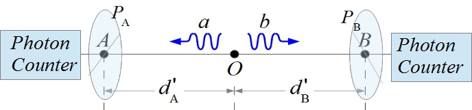
Figure 1: Two entangled photons a and b are generated at O and get the absorption polarizing films $P_{A}$ (Alice polarizer) and $P_{B}$(Bob polarizer). The photons passing through the polarizers are collected by photon counting modules. With $d^{\prime}_{A}$ and $d^{\prime}_{B}$ we denote the optical paths of photons a and b from source O to polarizers $P_{A}$ and $P_{B}$, respectively.

Analogous inequalities have been found by Clauser et al. (Clauser et al., 1969; Clauser and Horne, 1974). The Aspect experiment of 1982 (Aspect et al., 1982) demonstrated that the Bell inequality is not satisfied and also showed that quantum correlations cannot be explained in terms of subluminal or luminal communications. Many other experiments confirmed the Aspect results and some recent experiments finally closed the residual loopholes (Hensen et al., 2015; Giustina et al., 2015; Shalm et al., 2015; Rosenfeld et al., 2017). Then, the experimental results demonstrate that the local variables models cannot explain the quantum correlations between entangled particles. Some physicists suggested (Eberhard, 1989; Bohm and Hiley, 1993) that these correlations could be due to superluminal communications (v-causal models in nowadays literature (Gisin, 2014)). To avoid causal paradoxes, they assumed that a preferred frame (PF) exists where superluminal signals propagate isotropically with unknown velocity $v_{t}=\beta_{t}\>c$ ($\beta_{t}>1$). Below we will indicate the relativistic parameter $\beta_{t}=v_{t}/c$ as “the adimensional velocity”. Someone could be surprised for the existence of a preferred frame but references (Cocciaro, 2013, 2015) strongly stressed that the existence of a PF is not in the contrast with relativity. Furthermore, it has to be noticed that an universal PF has been already observed: it is the Cosmic Microwave Background frame (CMB frame) that moves at the adimensional velocity $\beta\approx 10^{-3}$ with respect to the Earth frame. It has been recently demonstrated an important theorem (Bancal et al., 2012; Barnea et al., 2013): v-causal models allow superluminal communications in the macroscopic world (signalling) if more than 2 entangled particles are involved. Although one of us believes that signalling is not incompatible with relativity (Cocciaro, 2013, 2015), most physicists think that there is no compatibility and that the experimental evidence of signalling would need a revision of relativity. In standard conditions, the superluminal communications lead to the usual QM correlations but there are special conditions (if the second particle reaches its measurement device when the collapsing wave didn’t yet reach it) where the QM correlations cannot be established and the Bell inequality should be satisfied. In fact, if the absorption polarizing films $P_{A}$ and $P_{B}$ in Figure 1 are at the same optical paths $d^{\prime}_{A}$ and $d^{\prime}_{B}$ from source O in the PF, the two photons get them simultaneously and there is no time to establish QM correlations. To verify this behavior, one can measure the correlation parameter $S_{max}$ defined as (Aspect, 2002; Cocciaro et al., 2017)

$$S_{max}=P_{0}-\sum_{i=1}^{3}P_{i}\;,$$ (2)

with $P_{0}=P\left(45\text{\textdegree},67.5\text{\textdegree}\right)$, $P_{1}=P\left(0\text{\textdegree},67.5\text{\textdegree}\right)$, $P_{2}=P\left(45\text{\textdegree},112.5\text{\textdegree}\right)$ and $P_{3}=P\left(90\text{\textdegree},22.5\text{\textdegree}\right)$, where $P(\alpha,\xi)$ is the probability that photon a passes through polarizer $P_{A}$ aligned at the angle $\alpha$ with respect to the horizontal plane and that photon b passes through polarizer $P_{B}$ aligned at the angle $\xi$. For any local variables model, $S_{max}$ must satisfy the modified Bell-Clauser-Horne-Shimony-Holt inequality $S_{max}\leq 0$ (Aspect, 2002; Cocciaro et al., 2017) whilst QM predicts $S_{max}=\nicefrac{{(\sqrt{2}-1)}}{{2}}\approx 0.2071$ for the entangled state in eq.(1). Probabilities $P(\alpha,\xi)$ can be experimentally obtained using the relation

$$P(\alpha,\xi)=\frac{N\left(\alpha,\xi\right)}{N_{tot}}\;,$$ (3)

where $N(\alpha,\xi)$ are the coincidences between entangled photons passing through the polarizers during the acquisition time $\Delta t$ and $N_{tot}$ is the total number of entangled photons couples that can be obtained using eq.(4):

$$N_{tot}=\sum_{i=0}^{3}N_{i}\;,$$ (4)

where $N_{0}=N\left(0\text{\textdegree},0\text{\textdegree}\right)$, $N_{1}=N\left(0\text{\textdegree},90\text{\textdegree}\right)$, $N_{2}=N\left(90\text{\textdegree},0\text{\textdegree}\right)$ and $N_{3}=N\left(90\text{\textdegree},90\text{\textdegree}\right)$. If $d\text{\textquoteright}_{A}=d\text{\textquoteright}_{B}$ in the PF, the quantum correlations cannot be established and $S_{max}$ should always satisfy the inequality $S_{max}\leq 0$ (Clauser et al., 1969; Clauser and Horne, 1974; Aspect, 2002; Cocciaro et al., 2017). Due to the experimental uncertainty $\Delta d\text{\textquoteright}$ on the equalization of the optical paths in the PF, the arrival times of the entangled photons at the polarizers could differ from one another for the quantity $\Delta t^{\prime}=\nicefrac{{\Delta d^{\prime}}}{{c}}$ and, thus, a superluminal communication would be impossible only if $\Delta t^{\prime}$ is lower than the communication time $d^{\prime}_{AB}/(\beta_{t}c)$, where $d^{\prime}_{AB}$ is the optical path from A to B in the PF (see Figure 1). The above condition is satisfied only if $\beta_{t}$ is lower than the maximum detectable adimensional velocity $\beta_{t,max}=\nicefrac{{d^{\prime}_{AB}}}{{\Delta d^{\prime}}}$ of the superluminal communications. Therefore, due to the $\Delta d\text{\textquoteright}$ uncertainty, a breakdown of quantum correlations ($S_{max}<0$) could be observed only if $\beta_{t}<\beta_{t,max}$. In the Earth frame the analysis becomes more complex. Indeed, the equalization of the optical paths $d_{A}$ and $d_{B}$ in the Earth frame does not imply their equalization also in the PF except if the unknown adimensional velocity vector $\overrightarrow{\beta}$ of the PF with respect to the Earth frame satisfies the orthogonality condition $\overrightarrow{\beta}\cdot\overrightarrow{AB}=0$. If the AB segment is East-West aligned, due to the Earth rotation around its axis, there are always two times $t_{1}$ and $t_{2}$ for each sidereal day where $\overrightarrow{AB}$ becomes orthogonal to $\overrightarrow{\beta}$ whatever is the orientation of the $\overrightarrow{\beta}$ vector (Salart et al., 2008a; Cocciaro et al., 2011). At these times, the quantum correlations should not be established and $S_{max}$ should exhibit a breakdown from the quantum value $S_{max}=0.2071$ toward $S_{max}\leq 0$ if the superluminal adimensional velocity $\beta_{t}$ is lower than $\beta_{t,max}$. However, an acquisition time $\Delta t$ has to be spent to measure parameter $S_{max}$ and, thus, the orthogonality condition $\overrightarrow{\beta}\cdot\overrightarrow{AB}=0$ can be only approximately satisfied during this acquisition time. This leads to a further contribution to the uncertainty $\Delta t^{\prime}$ on the arrival times of the entangled photons at the two polarizers in the preferred frame. Then, in the Earth experiment, the maximum detectable velocity $\beta_{t,max}$ is affected both by the uncertainty $\Delta d$ on the equalization of the optical paths and by the acquisition time $\Delta t$. Smaller ones are $\Delta d$ and $\Delta t$ and bigger is $\beta_{t,max}$. Using the relativistic Lorentz equations one finds (Salart et al., 2008a; Cocciaro et al., 2011)

$$\beta_{t,max}=\sqrt{1+\frac{\left(1-\beta^{2}\right)\left[1-\rho^{2}\right]}{\left[\rho+\frac{\pi\beta\delta t}{T}\sin\chi\right]^{2}}}\;,$$ (5)

where $\chi$ is the unknown angle that the velocity of the PF makes with the Earth rotation axis, T is Earth rotation day and $\rho=\nicefrac{{d_{AB}}}{{\Delta d}}$ , where $d_{AB}$ is the optical path between points A and B in the Earth Frame. Parameter $\delta t$ ($\delta t/T\ll 1$) in eq.(5) has been usually assumed to coincide with time $\Delta t$ needed for a complete measurement of $S_{max}$ but this is not correct. Indeed, if $t_{i}$ (i =1,2) are the daily times where the orthogonality condition $\overrightarrow{\beta}\cdot\overrightarrow{AB}=0$ is satisfied, the superluminal model predicts that no communication is possible in the time intervals $I_{i}=\left[t_{i}-\delta t/2,\>t_{i}+\delta t/2\right]$ if $\beta_{t}<\beta_{t,max}$ (Salart et al., 2008a; Cocciaro et al., 2011). Unfortunately, times $t_{i}$ are unknown and the acquisitions cannot be synchronized with them. Then, one can be sure that a full acquisition interval $\Delta t$ is certainly contained in the unknown $I_{i}$ interval only if $\Delta t\leq\delta t/2$. This means that parameter $\delta t$ in eq.(5) is given by

$$\delta t=2\,\Delta t\;.$$ (6)

Some experimental tests of the superluminal models have been reported in the literature but, so far, no evidence for a violation of QM predictions has been found and only lower bounds $\beta_{t,max}$ have been established (Salart et al., 2008a; Cocciaro et al., 2011; Yin et al., 2013; Cocciaro et al., 2017). In reference (Yin et al., 2013) the locality and freedom-of-choice loopholes were also addressed. Here we report the results of a new experiment where the loopholes above are not taken into account but the maximum detectable velocity of the superluminal communications is increased by about two orders of magnitude. In particular, according to (Salart et al., 2008b) we here test the “assumption that quantum correlations are due to supra-luminal influences of a first event onto a second event”. Since we use absorption polarizing films, we assume that the above events are the collapses of the polarization state that occur when photons hit the absorption polarizers.

I EXPERIMENTAL METHOD

I.1 The experimental apparatus and procedures.

Our experimental apparatus, the procedures used to get very small values of the basic experimental parameters $\rho$ and $\Delta t$ and the experimental uncertainties have been described in detail in a previous paper (Cocciaro et al., 2017) and, thus, we will remind here only the main features.

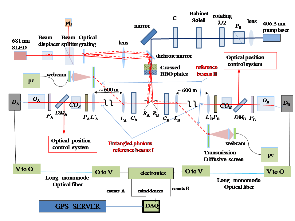
Figure 2: Schematic view of the experimental apparatus. Note that the figure is not to scale and, in particular, the distances between lenses $L_{A}\thinspace\mathrm{and}\thinspace L_{B}$ and $\thinspace L^{\prime}_{A}$ and $L^{\prime}_{B}$ ($\approx 600\thinspace\mathrm{m}$) are much larger then all the other distances. To simplify the drawing some details have not be inserted in the figure. The 220 mW pump beam with wavelength $\lambda_{p}=$406.3 nm (blue thick full line in the figure) is polarized by the polarizer $P_{0}$ and the $\lambda/2$ plate. The Babinet-Soleil compensator introduces a variable optical dephasing between the horizontal and vertical polarizations. $C$, $C_{A}$ and $C_{B}$ are anisotropic compensator plates used to get a high intensity source of entangled photons with a sufficient fidelity. $R_{A}$ and $R_{B}$ are right angle prisms. The pump beam is focused at the centre of two crossed adjacent BBO plates (29.05° tilt angle) where entangled photons having wavelength $\lambda=$812.6 nm are generated and emitted at the angles $\pm 2.42\text{\textdegree}$ with respect to the pump laser beam. $L_{A},\thinspace L_{B},\thinspace L^{\prime}_{A}$ and $L^{\prime}_{B}$ are specially designed $15\thinspace\text{cm}$-diameter achromatic lenses aligned along the EGO gallery and having a $6.00\thinspace\text{m}$ focal length at both the 812.6 nm and 681 nm wavelengths. $P_{A}$ and $P_{B}$ are absorption polarizing filters. $O_{A}$, $O_{B}$, $CO_{A}$ and $CO_{B}$ are systems of lenses. $DM_{A}$ and $DM_{B}$ are dichroic mirrors, $F_{A}$ and $F_{B}$ are sets of adjacent optical filters, $D_{A}$ and $D_{B}$ are photon counting detectors. The superluminous diode (SLED) having wavelength $\lambda_{R}$= 681 nm and coherence length 28.1 ${\textstyle\mu m}$, the beam displacer and the optical grating are used to produce two reference beams in each arm of the EGO gallery (full and broken red lines) as discussed in the text. V to O denote electronic systems that transform the output voltage pulses produced by the photon counting detectors into optical pulses, whilst O to V transform the optical pulses into voltage pulses. DAQ is a National Instruments CompactDAC that provides a real time acquisition of coincidences.

To reach a high value of $\beta_{t,max}$, one has to make parameters $\rho$ and $\delta t$ in eq.(5) as smaller as possible. We get a small value of $\rho=\nicefrac{{d_{AB}}}{{\Delta d}}$ performing our measurements in the so called "East-West" gallery of the European Gravitational Observatory (EGO)(European Gravitational Observatory,https://www.ego-gw.it/, ) of Cascina ($d_{AB}\approx 1200$ m) and we use an interferometric method to equalize the optical paths $d_{A}$ and $d_{B}$ ($d_{A}\approx d_{B}\approx 600$ m). The final uncertainty $\Delta d$ on the equality of the optical paths is due to many error sources including the finite thickness of the polarizing layers, the air dispersion and the uncertainty on the interferometric measurement. As shown in reference (Cocciaro et al., 2017), the estimated uncertainty is $\Delta d\approx 0.22$ mm. To reduce the acquisition time we need a high intensity source of entangled photons in a sufficiently pure entangled state. We get this goal using the compensation procedures developed by the Kwiat group (Altepeter et al., 2005; Akselrod et al., 2007; Rangarajan et al., 2009) and developing a proper optical configuration that ensures low losses of entangled photons along the gallery. Unfortunately, the EGO gallery is not aligned along the East-West axis but makes the angle $\gamma=18\text{\textdegree\ }$ $=\pi/10$ with it. Then, one easily infers that the orthogonality condition $\overrightarrow{\beta}\cdot\overrightarrow{AB}=0$ can be never satisfied if the velocity vector of the PF makes a polar angle $\chi<\gamma=\pi/10$ or $\chi>\pi-\gamma=9\pi/10$ with respect to the Earth rotation axis. This means that our experiment is virtually insensitive to a fraction $\Omega/(4\,\pi)=\int_{{}_{0}}^{\gamma}\sin\theta d\theta<5\%$ of all the possible alignments of the PF velocity vector. For a detailed analysis of the case $\gamma\neq 0$ we refer the reader to reference (Salart et al., 2008a). Note that the Reference Frame of the Cosmic Microwave Background ($\chi\approx 97\text{\textdegree}$) is accessible to our experiment. Eq.(5) was obtained under the assumption that the experiment is aligned along the East-West axis ($\gamma=0$) but, for $\gamma\geq 0$ and $\pi-\gamma\geq\chi\geq\gamma$, it has to be replaced by (Salart et al., 2008a)

$$\beta_{t,max}=\sqrt{1+\frac{\left(1-\beta^{2}\right)\left[1-\rho^{2}\right]}{\left[\rho+A\,\frac{\pi\beta\delta t}{T}\right]^{2}}}\;,$$ (7)

where coefficient A is defined as

$$A=\sqrt{\sin^{2}\chi\cos^{2}\gamma-\cos^{2}\chi\sin^{2}\gamma}\>.$$ (8)

Velocity $\beta_{t,max}$ greatly decreases out of the interval $\pi-\gamma\geq\chi\geq\gamma$(Salart et al., 2008a).

A schematic view of the experimental apparatus is shown in figure 2. A pump laser beam at a wavelength $\lambda_{p}=$406.3 nm is generated by the 220 mW laser diode shown at the top right in figure 2. The pump beam passes through an achromatic lens, a Glan-Thompson polarizer, a motorized $\lambda/2$ plate, a motorized Babinet-Soleil compensator and a quartz plate C. Then, it is reflected by a mirror, passes through a 565 nm short pass dichroic mirror (Chroma T565spxe) and is focused (spot diameter = 0.6 mm) at the center of two thin (thickness $\approx 0.56$ mm) adjacent crossed BBO nonlinear optical crystals plates (29.05° tilt angle) cut for type I phase matching (Kwiat et al., 1999). The BBO plates have the optical axes lying in the horizontal and vertical plane, respectively. The $\lambda/2$ plate aligns the polarization of the incident pump beam at 45° with respect to the horizontal axis. The quartz plate C compensates the effects due to the low coherence of the pump beam ($\approx$ 0.2 mm coherence length) (Rangarajan et al., 2009). Down conversion leads to two outgoing beams of entangled photons at the average wavelength $\lambda=2\,\lambda_{p}=812.6\,\textrm{nm}$ that mainly propagate at two symmetric angles ($\pm 2.4\text{2\textdegree}$) with respect to the normal to the crossed BBO plates. A proper adjustment of the optical dephasing induced by the Soleil-Babinet compensator provides the polarization entangled state in eq.(1). The entangled beams are deviated in opposite directions along the EGO gallery by two right-angle prisms ($R_{A}$ and $R_{B}$) and passe through the BBO compensating plates $C_{A}$ and $C_{B}$. The Kwiat compensating plates C, $C_{A}$ and $C_{B}$ are used to get a high intensity source of entangled photons ($N_{tot}\approx 23000$ coincidences/s) in an entangled state of sufficient purity (Altepeter et al., 2005; Akselrod et al., 2007; Rangarajan et al., 2009). The entangled beams, propagating along opposite directions, impinge on polarizers $P_{A}$ and $P_{B}$ at a distance of about 600 m from the source. Our experiment requires the equalization of the optical paths $d_{A}$ and $d_{B}$ between the source of the entangled photons and polarizers $P_{A}$ and $P_{B}$ and needs stable coincidences counts during the whole measurement time ($\approx$ 8 days). Both these requirements are satisfied using four reference beams at wavelength $\lambda_{R}=$681 nm that are utilized to align the optical system, to equalize the optical paths and to compensate the deviations of the entangled beams due to the air refractive index gradients induced by sunlight on the top of the gallery. The four reference beams are obtained starting from the collimated beam emitted by the 3 mW superluminous diode (SLED) shown at the top left in figure 2. The beam passes through a beam displacer (Thorlabs BDY12U) that splits the incident beam into two parallel beams (I and II) at a relative distance of 1.2 mm. Beam I is represented by a full line in the figure whilst beam II by a broken line. Beams I and II are focused (spot diameter $\approx 0.3$ mm) orthogonally on a transmission phase grating that mainly produces +1 e -1 diffracted beams at the diffraction angles $\pm$ 2.43° that are virtually coincident with the average emission angles of the entangled photons ($\pm$2.42°). An achromatic lens (150 mm focal length) projects on the crossed BBO plates a 1:1 image of the spots of beams I and II occurring on the grating. The spot of beam I is centered within $\approx\pm 0.03\>{\textstyle mm}$ with respect to the pump beam spot where the entangled photons are generated (the “source” of the entangled photons). Then, beams I outgoing from the crossed BBO plates virtually follows the same paths of the entangled beams. The whole system described above lies on an optical table and is enclosed in a large box that ensures a fixed temperature $T=24\text{\textdegree C}\pm 0.1\text{\textdegree C}$ by circulation of Para-flu fluid. Two 80 W fans ensure a sufficient temperature uniformity. The entangled beams and the reference beams are collected by large diameter (15 cm) achromatic lenses $L_{A}$ and $L_{B}$ that have been built to have the same focal length at the wavelengths of the reference and the entangled beams (6.00 m at $\lambda_{R}=681\,\textrm{nm and }$$\lambda=812.6\,\textrm{nm}$). These beams propagate along the gallery arms and impinge on two identical achromatic lenses $L^{\prime}_{A}$ and $L^{\prime}_{B}$ at a distance $\approx$ 600 m from the source of the entangled photons. Real 1:1 images (0.6 mm-width) of the source and of the spot of beam I occurring on the crossed BBO plates are produced at the centers of the linear polarizers layers $P_{A}$ and $P_{B}$ (Thorlabs LPNIR ). Beams II are slightly deviated by lenses $L_{A}$ and $L_{B}$ and impinge on two diffusing screens put adjacent to lenses $L^{\prime}_{A}$ and $L^{\prime}_{B}$. The diffused light outgoing from each screen is collected by a webcam connected to a PC and a Labview program calculates the position of the diffusing spot. The daily displacements of the above spots (up to 1.2 m in a Summer day) due to air refractive index gradients induced by sunlight are compensated using a proper feedback where lenses $L_{A}$ and $L_{B}$ are moved orthogonally to their optical axes to maintain fixed the position of the spots on the diffusing screens (see Section 2.2 in reference (Cocciaro et al., 2017) for details). This procedure ensures that beams I and, thus, the entangled beams remain virtually centered with respect to lenses $L^{\prime}_{A}$ and $L^{\prime}_{B}$. The reference beams I outgoing from polarizers $P_{A}$ and $P_{B}$ are almost fully reflected by the long pass dichroic mirrors $DM_{A}$ and $DM_{B}$ (Chroma T760lpxr) and enter the optical position control systems that measure the position and the astigmatism of the beam spots on the polarizers. Using a Labview program operating in a PC, lenses $L^{\prime}_{A}$ and $L^{\prime}_{B}$ are moved orthogonally to their optical axes to maintain the spot position at the center of the polarizers within $\pm 0.4$ mm during the whole measurement time. An other program controls the astigmatism of the images using the variable-focus cylindrical lenses $CO_{A}$ and $CO_{B}$. The equalization of the optical paths $d_{A}$ and $d_{B}$ is obtained exploiting the beams I that are partially reflected by the polarizing layers $P_{A}$ and $P_{B}$ and that come back producing interference on the photodetector Ph shown on the top left in Figure 2. Details on the feedback procedures and on the interferometric method can be found in Section 2.2 and 2.3 of reference (Cocciaro et al., 2017), respectively. Each of the entangled photons beams outgoing from the two polarizers passes through the long pass dichroic mirror ($DM_{A}$ or $DM_{B}$ in the Figure) and a filtering set ($F_{A}$ or $F_{B}$ in the Figure) made by two long-pass optical filters ( Chroma ET765lp filters ; $\lambda_{c}=765\,\mathrm{nm}$) that stop the reference 681 nm beams and a band-pass filter ( Chroma ET810/40m ; $\lambda=810\,\mathrm{nm}\pm 20\,\mathrm{nm}$). Then, each beam is focused by a system of optical lenses ($O_{A}$ or $O_{B}$ ) on a $200\,\mu m$ multimode optical fiber having a large numerical aperture (0.39) connected to a Perkin Elmer photons counter module. The output pulses of the photons counters are transformed into optical pulses (using the LCM155EW4932-64 modules of Nortel Networks) that propagate in two monomode optical fibers toward the central optical table where the entangled photons are generated. Finally, the optical pulses are transformed again into electric pulses and sent to an electronic coincidence circuit. An electronic counter connected to a National Instruments CompactDAQ counts the Alice pulses $N_{A}$, the Bob pulses $N_{B}$ and the coincidences pulses N.

B. The fast acquisition procedure.

In our preliminary experiment (Cocciaro et al., 2017), the measurements of the probabilities appearing in eq.(2) were made sequentially: a PC connected to precision stepper motors rotated polarizers $P_{A}$ and $P_{B}$ up to reach the first couple of angles $\alpha$ and $\beta$ appearing in eq.(2) ($\alpha$ = 45° and $\beta$= 67.5°) and the corresponding coincidences $N(\alpha,\beta)$ were acquired with an acquisition time of 1 s, then the successive couple of $\alpha$ and $\beta$ angles was set and the corresponding coincidences were acquired and so on. When all the eight contributions $N(\alpha,\beta)$ entering in equations (2) and (4) were obtained, the program calculated $S_{max}$. This procedure needed many consecutive rotations of the polarizers before a single value of $S_{max}$ was obtained leading to a long acquisition time interval $\Delta t\approx$100 s for each measurement of $S_{max}$. To greatly reduce $\Delta t$ and increase the maximum detectable adimensional velocity $\beta_{t,max}$, we exploits here the daily periodicity of the investigated phenomenon and we measure each of the four contributions appearing in eq.(2) in successive daily experimental runs. This procedure allows us to set the polarization angles $\alpha$ and $\xi$ only one time each day before starting the measurement of $P_{i}$. Then, any retardation due to the polarizers rotation is avoided. Furthermore the PC used in our previous experiment has been replaced here by a National Instruments CompactDAQ where a Real Time Labview program runs. This new procedure ensures a full continuity of the acquisitions and a constant acquisition time. The obtained experimental values of the basic parameters $\rho$ (see (Cocciaro et al., 2017)) and $\delta t$ appearing in eq.(5) are

$$\rho=1.83\times 10^{-7}\;\;and\;\;\delta t=2\,\Delta t=0.494\,\textrm{s}$$ (9)

that provide a $\beta_{t,max}$ value about two orders of magnitude higher than the those obtained in previous experiments. A GPS Network Time Server (TM2000A) provides the actual UTC time (P.K. Seidelmann, 1992; UT, 1) with an absolute accuracy better than 1 ms also if the connection to the satellites is lost up to a 80 hours time. Since the investigated phenomenon is related to the Earth rotation, we synchronize the acquisitions with the Earth rotation time $t=\theta\times 240\,\textrm{s}$ where $\theta$ is the Earth Rotation Angle(ERA (P.K. Seidelmann, 1992; UT, 1)) expressed in degrees. The ERA time is the modern alternative to the Sidereal Time and it is given by $t=86400\times(\mathrm{TJ\>mod}\>1)$ where “mod” represents the modulo operation and $TJ=\left[a_{1}+b_{1}\times\left(\textrm{Julian\,UT1\,day}-2451545.0\right)\right]$ with $a_{1}=0.7790572732640$ days and $b_{1}=1.00273781191135448$. The Julian UT1 day is strictly related to the UT1 time that takes into account for the non uniformity of the Earth rotation velocity and, thus, does not coincide with the UTC atomic time provided by the GPS. The IERS Bullettin A (IER, ) provides the value of the daily difference $\Delta=UT1-UTC$ and, thus, the UT1 and the ERA time can be calculated. We decide to start each acquisition run at the Greenwich ERA time $t=0$.

The successive steps of the fully automated procedure are:

1- The GPS Greenwich UTC time and the UT1-UTC value are acquired, then, the Greenwich ERA time t is calculated. Successively, the UTC time that corresponds to the next zero value of the Greenwich ERA time is calculated.

2- Two hours before the occurrence of $t=0$, we measure the total number of couples of entangled photons $N_{tot}$. The program rotates the $P_{A}$ and $P_{B}$ polarizers and sets successively the $\alpha$ and $\xi$ angles that enter the expression of the total number of incident entangled couples $N_{tot}$ in eq.(4). For each setting of the polarizers angles, the coincidences are measured for a sufficiently long acquisition time interval (100 s) to made negligible the counts statistical noise with respect to others noise sources. The spurious statistical coincidences $N_{S}=N_{A}\times N_{B}\times T_{p}/\Delta t$ are subtracted, where $T_{p}$ is the pulses duration time and $\Delta t$ is the acquisition time interval. The value $T_{p}=$ 29.2 ns is obtained from a calibration procedure where coincidences between totally uncorrelated photons are detected. Finally, the total number of entangled photons $N_{tot}$ is calculated using eq.(4).

3- At the end of these preliminary measurements, the polarizers angles are set at the values $\alpha$= 45° and $\xi$=67.5° appearing in the first contribution $P_{0}$ in eq.(2). Then, the acquisition of the coincidences starts at the Greenwich ERA time $t=$0. The duration of a complete acquisition run is $T_{0}=$ 36 ERA hours that correspond to about 35 h ; 54 min and 7 s in the standard $UTC$ time. $2^{19}$ successive acquisitions are made in each acquisition run with the acquisition time interval $\Delta t=\nicefrac{{T_{0}}}{{2^{19}}}\simeq 246.517461\,\textrm{ms}$ ( in standard $UTC$ unities). Note that, due to the daily small changes of the $UT1-UTC$ difference, $\Delta t$ exhibits small daily variations (the maximum variation was $\approx$ 0.000001 ms in the whole measurement time). To ensure a time precision better than 1 ms, the microseconds internal counter of the Real Time Labview is used and the GPS server is interrogated every 5 minutes. Furthermore, a suitable subroutine partially correct ( within 0.1 ms) time errors introduced by the microseconds quantization of the DAQ clock.

4- At the end of the first acquisition run, the program calculates the $2^{19}$ values of $P_{0}$ and sets the second couple of angles $\alpha$ and $\xi$ appearing in the $P_{1}$ term in eq.(2). Then, steps 3 and 4 are repeated until all probabilities $P_{i}$ entering eq.(2) are obtained. To appreciably reduce the residual spurious effects due to air turbulence induced by sunlight on the top of the gallery, all the measurements were performed during the 2017 autumn season starting at the 0 ERA hour of October 24 and stopping at the 12 ERA hour of October 31.

II RESULTS AND CONCLUSIONS

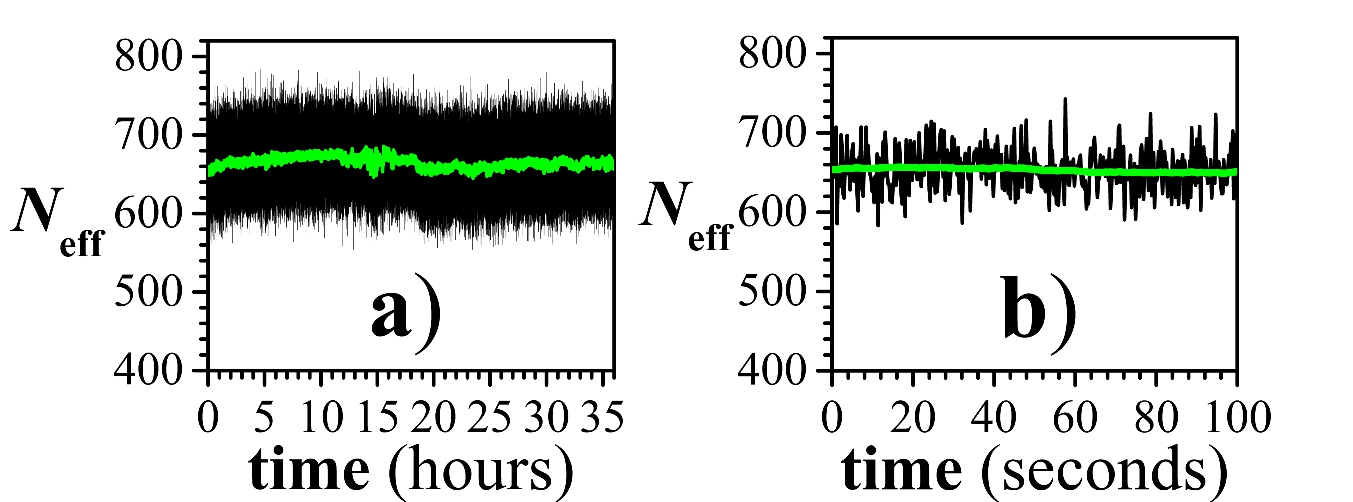
Figure 3: a) An example of the effective coincidences (true + spurious) versus the Greenwich ERA time. The $2^{19}$ points are connected by black lines leading to the resulting black region in the Figure. The acquisition time of coincidences is $\Delta t\approx 0.246\,\textrm{s}$ in standard $UTC$ unities. The green full line is the result of smoothing averaging over 200 adjacent points. The slow variations in the smoothing curve are caused by residual noise due to sunlight on the top of the gallery. b) A detail of the coincidences during 100 s is shown.

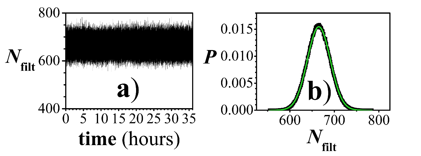
Figure 4: a) “Filtered” coincidences $N_{filt}=N_{eff}-N(smoothing)+<N_{eff}>$ where the slow instrumental drift of the average value in Figure 3 has been subtracted. The acquisition time of coincidences is $\Delta t\approx 0.246\,\textrm{s}$ and the total number of acquisitions is $2^{19}$. b) probability distribution of the coincidences (black points). The full green curve does not represents a best fit but it is the normal distribution predicted by the statistic theory of counts having $\sigma^{2}=<N_{filt}>=665.042$ with no free parameters.

Figure 3(a) shows an example of the effective coincidences (true+spurious) $N_{eff}$ versus the Greenwich ERA time during a single run. The green full line is the result of a smoothing obtained averaging over 200 adjacent points while a detail of the coincidences during 100 s is shown in Figure3(b). The small slow changes that are visible in the smoothing curve are strictly related to the daily small residual displacements of the entangled photons beams induced by sunlight. The greater contribution to noise in our experiment is the statistical counts noise, while the other noise sources are virtually negligible. This is evident if we eliminate the slow fluctuations plotting the “filtered” coincidences $N_{filt}=N_{eff}-N(smoothing)+<N_{eff}>$. Figure 4(a) shows $N_{filt}$ versus the Greenwich ERA time whilst Figure 4(b) shows the correspondent probability distribution P (black points). We emphasize here that the full green line in Figure 4(b) is not a best fit but it is the Normal Gaussian function with parameters $\sigma$ and $<N_{filt}>$ that are predicted by the Statistics of counts and are given by $\sigma^{2}=<N_{filt}>=665.042$. Figures 5(a)-5(d) show the probabilities $P_{i}=P(\alpha_{i},\xi_{i})=\nicefrac{{N(\alpha_{i},\xi_{i})}}{{N_{tot}}}$ obtained in the successive runs where the spurious coincidences $N_{S}=N_{A}\times N_{B}\times T_{p}/\Delta t$ have been subtracted but no filtering was performed. The black region represents the measured values, the full green line represents the average value whilst the green dotted line represents the value predicted by QM for the pure entangled state in eq.(1) (fidelity $F=1$). The discrepancy between the full and dotted lines indicates that our entangled state is not completely pure ($F<1$) or that some systematic noise is present. In the simplest and rough assumption that the breakdown of quantum correlations occurs with exactly the Earth rotation periodicity one could calculate a $S_{max}$ value at each ERA time by substituting the $P_{i}$ contributions of Figures 5 measured at the same ERA time t during different experimental runs into the theoretical expression of $S_{max}$ in eq.(2).

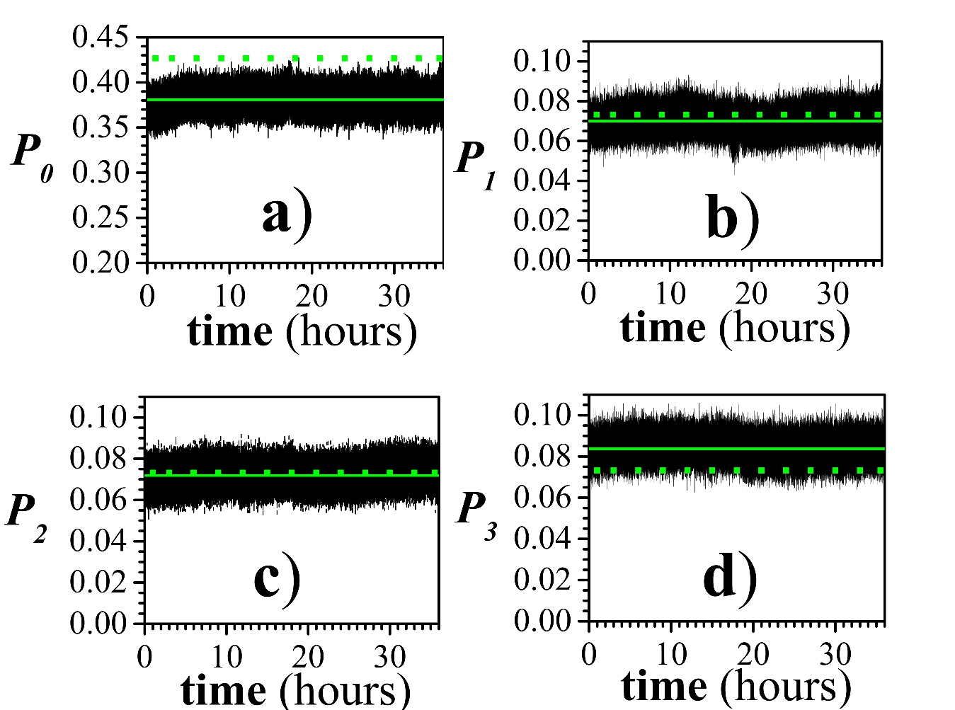
Figure 5: Probabilities $P_{0},\,P_{1},\,P_{2}\,\mathrm{and\>}P_{3}$ measured in successive runs versus the Greenwich ERA time. The $2^{19}$ measured values are connected by straight lines leading to the resulting black regions in the Figure. The acquisition time is $\Delta t\approx 0.246\,\textrm{s}$. The green full lines represent the average values of the measured probabilities: $<P_{0}>=0.38087$, $<P_{1}>=0.06999$, $<P_{2}>=0.07187$, $<P_{3}>=0.08378$. The green dotted lines correspond to the values predicted by QM for a pure entangled state: $P_{0}=0.4267$, $P_{1}=P_{2}=P_{3}=0.0732$. The difference between dotted and full lines indicates that our state is not a pure entangled state or that some instrumental noise occurs.

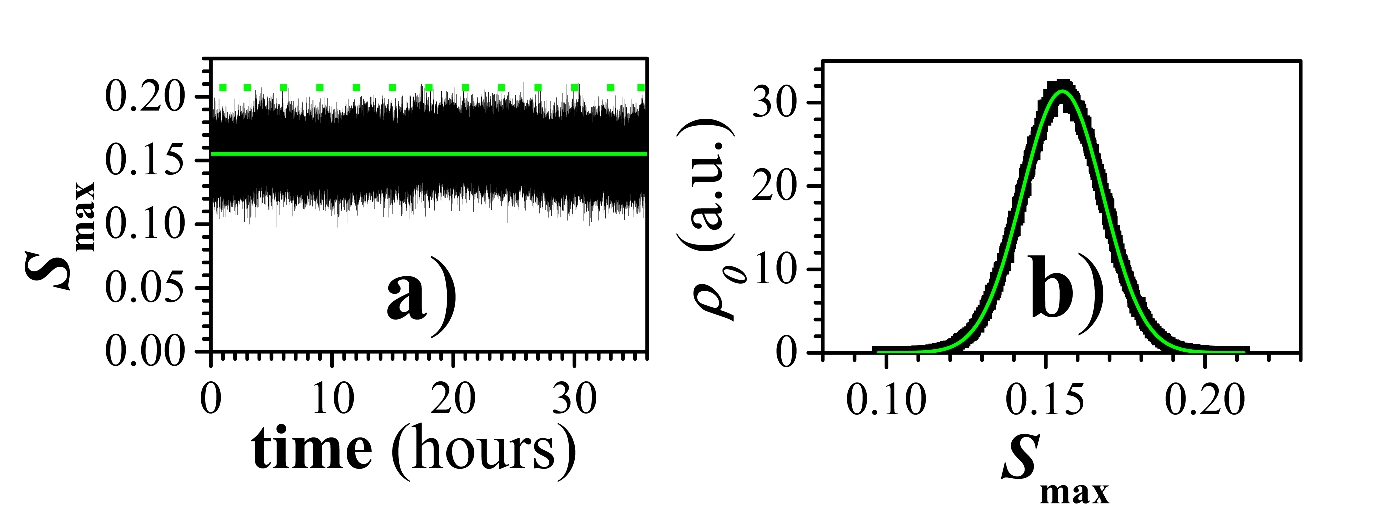
Figure 6: a) $S_{max}$ versus the ERA time obtained using the relation $S_{max}(t)=P_{0}(t)-P_{1}(t)-P_{2}(t)-P_{3}(t)$. The green full line is the average value $<S_{max}>=0.15523$, whilst the green dotted line represents the QM average value $<S_{max}>=0.207$ characterizing the pure entangled state in eq.(1). The difference between dotted and full lines indicates that our state is not a pure entangled state. However, the average value $<S_{max}>=0.15523$ is sufficiently greater than zero to allow an accurate test of the Bell inequality. b) The Frequency Distribution $\rho_{0}$ of the $2^{19}$ measured values of $S_{max}$ in arbitrary units is shown. The full green curve is the Gaussian fit with standard deviation $\sigma=0.01272$ and $<S_{max}>=0.15523$.

With this procedure we get the results shown in Figure 6(a) (black region) and the corresponding frequency distribution $\rho_{0}$ shown in Figure 6(b) where black points represent the experimental results whilst the full green line is the best fit with the Gaussian function $A\exp\left[\nicefrac{{-\left(S_{max}-<S_{max}>\right)^{2}}}{{\left(2\sigma^{2}\right)}}\right]$ with standard deviation $\sigma=0.01272$ and $<S_{max}>=0.15523$. The green full line in Figure 6(a) shows the average value $<S_{max}>$ whilst the green dotted line is the value $S_{max}=$ 0.2071 predicted by QM for the pure entangled state in eq.(1)($F=1$). No breakdown of $S_{max}$ to zero is visible in Figure 6(a) and the lowest experimental values of $S_{max}$ are at more then 7 standard deviations from the maximum value $S_{max}=0$ predicted by local variables models. However, the analysis above is not sufficient to conclude that no superluminal effect is present. In fact, the breakdown of the QM correlations is predicted to occur at the two times where $\overrightarrow{\beta}\cdot\overrightarrow{AB}=0$, where $\overrightarrow{\beta}$ is the adimensional velocity vector of the PF with respect to Earth. Due to the revolution motion of the Earth around the sun and other motions (precession and nutation of the Earth axis), vector $\overrightarrow{\beta}$ does not come back exactly at the same orientation with respect to the Earth frame after one ERA day. Then, the orthogonality condition is not satisfied exactly at the same ERA times in different ERA days but some unknown time shift can occur (shifts lower than a few min/day can be expected). Then, a rigorous test of the v-causal models requires a completely different analysis of the experimental data. Denote by $t_{i1}$ and $t_{i2}$ the two unknown times during the i-th measurement run ($i=0-3$) where the orthogonality condition $\overrightarrow{\beta}\cdot\overrightarrow{AB}=0$ is satisfied and by $P_{i}(t_{ij})$ with $i=0-3$ and $j=1,2$ the corresponding probabilities measured at these times. According to the v-causal models, if $\beta_{t}<\beta_{t,max}$ all or someone of these probabilities should be different from the QM values and, thus, the correlation parameters

$$S_{max}\left(j\right)=P_{0}\left(t_{0j}\right)-\sum_{i=1}^{3}P_{i}\left(t_{ij}\right)\;,$$ (10)

with $j=1,2$, should satisfy the Bell inequality $S_{max}\left(j\right)\leq 0$ if $\beta_{t}$$<\beta_{t,max}$.

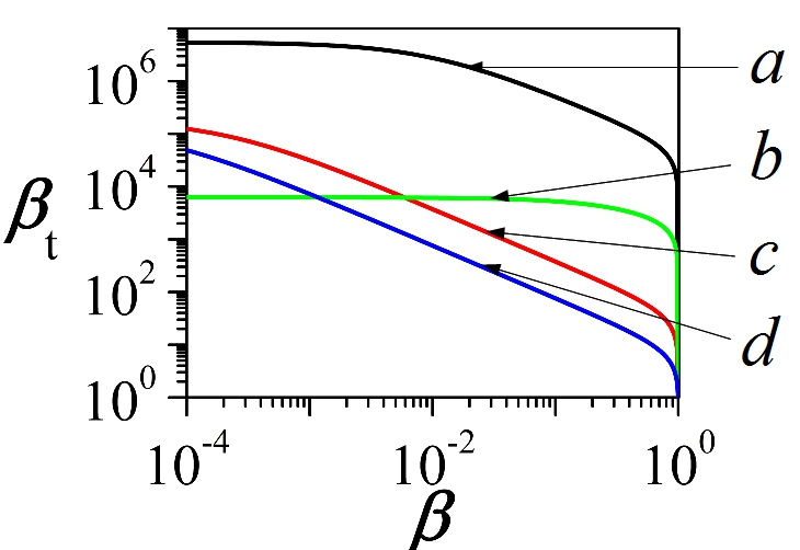
Figure 7: Curve a shows the $\beta_{t,max}$ values obtained in our experiment using eq.7 ($\rho=1.83\times 10^{-7}$, $\delta t=2\,\Delta t=0.494\>{\textstyle s}$ and $\gamma=18\text{\textdegree}$) versus the unknown adimensional velocity $\beta$ of the PF for the unfavorable case $\chi=\nicefrac{{\pi}}{{2}}$; curve b is the result obtained in reference (Cocciaro et al., 2011) ($\rho=1.6\times 10^{-4}$, $\delta t=2\,\Delta t=8\>{\textstyle s}$ and $\gamma=0\text{\textdegree}$); curve c is the result obtained in reference (Salart et al., 2008a) ($\rho=5.4\times 10^{-6}$, $\delta t=2\,\Delta t=720\>{\textstyle s}$ and $\gamma=5.9\text{\textdegree}$) and curve d that obtained in reference (Yin et al., 2013) ($\rho=7.3\times 10^{-6}$, $\delta t=2\,\Delta t=3600\>{\textstyle s}$ and $\gamma=0\text{\textdegree}$). Note that only in the case of curve d also the locality and the freedom-of-choice loopholes were addressed.

We do not know times $t_{ij}$ and we cannot calculate $S_{max}(j)$ but it is obvious from eq.(10) that $S_{max}\left(j\right)\geq S=MIN\left(P_{0}\right)-MAX\left(P_{1}\right)-MAX\left(P_{2}\right)-MAX\left(P_{3}\right)$ where $MIN\left(P_{i}\right)$ and $MAX\left(P_{i}\right)$ denote the absolute minimum and maximum measured values of $P_{i}$, respectively. From the data in Figures 5 we get $S=0.04237$ and, thus, $S_{max}\left(j\right)\geq 0.04237\approx 3.3\>\sigma$. This means that the probability that a value of $S_{max}\left(j\right)$ lower or equal to zero could be compatible with our measured values is $p\leq\frac{1}{2}\mathrm{erfc}\left[\nicefrac{{0.04237}}{{\left(\sqrt{2}\sigma\right)}}\right]=4.3\cdot 10^{-4}$, where $\textrm{erfc}\left(x\right)$ is the complementary error function. The superluminal models predict that at the least two breakdowns of $S_{max}$ must occur in the 36 h time and, thus, the probability that both these breakdowns happen here is $p\leq p^{2}\sim 2\times 10^{-7}$. Then, we can conclude that no evidence for the presence of superluminal communications is found and only a higher value of the lower bound $\beta_{t,max}$ can be established. Substituting the experimental values $\rho=1.83\times 10^{-7}$ and $\delta t=2\,\Delta t=0.494\,\textrm{s}$ in eq.(7) one obtains $\beta_{t,max}$ as a function of the unknown modulus $\beta$ ($\beta<1$ ) of the adimensional velocity of the Preferred Frame and of his angle $\chi$ with respect to the Earth rotation axis. We remind that eq.(7) holds only if angle $\chi$ is inside the interval $\left[\gamma,\pi-\gamma\right]$ where $\gamma=\pi/10$ rad, whilst $\beta_{t,max}$ sharply decreases out of this interval (Salart et al., 2008a). According to eq.(7), $\beta_{t,max}$ reaches the maximum value at the borders $\chi=\gamma$ and $\chi=\pi-\gamma$ and the minimum value at $\chi=\pi/2$ . The upper curve in Figure 7 shows our $\beta_{t,max}$ versus the unknown adimensional velocity $\beta$ of the PF in the unfavorable case $\chi=\pi/2$. For PF velocities comparable to those of the CMB Frame ($\beta\approx 10^{-3})$ the corresponding lower bound is $\beta_{t,max}\approx 5\times 10^{6}$. The lower curves represent the experimental values of $\beta_{t,max}$ obtained in the previous experiments (Salart et al., 2008a; Cocciaro et al., 2011; Yin et al., 2013). No breakdown of quantum correlations has been observed and, thus, we can infer that either the superluminal communications are not responsible for quantum correlations or their adimensional velocities are greater than $\beta_{t,max}$. Finally, it has to be noticed that it remains open the possibility that $\beta_{t}$$<\beta_{t,max}$ but vector $\overrightarrow{\beta}$ makes a polar angle $\chi<\gamma=\pi/10$ or $\chi>\pi-\gamma=9\pi/10$ with the Earth rotation axis.