Global-local mixing for the Boole map

Abstract

In the context of ‘infinite-volume mixing’ we prove global-local mixing for the Boole map, a.k.a. Boole transformation, which is the prototype of a non-uniformly expanding map with two neutral fixed points. Global-local mixing amounts to the decorrelation of all pairs of global and local observables. In terms of the equilibrium properties of the system it means that the evolution of every absolutely continuous probability measure converges, in a certain precise sense, to an averaging functional over the entire space.

Mathematics Subject Classification (2010): 37A40, 37A25, 37D25, 37C25.

1 Introduction

In 1857 G. Boole [3] proved that

$$\int_{-\infty}^{\infty}f(x)\,dx=\int_{-\infty}^{\infty}f\!\left(x-\frac{1}{x}\right)dx,$$ (1)

whenever one of the two sides makes sense. He obtained this result by investigating changes of variables of the type $x-\frac{\lambda_{1}}{x-\lambda_{2}}$, for $\lambda_{1},\lambda_{2}\in\mathbb{R}$, which were extremely helpful in evaluating indefinite integrals, especially when complex contour integration was no trivial matter. In this note we look at some properties of the Boole map $T:\mathbb{R}\to\mathbb{R}$ where

$$T(x):=x-\frac{1}{x}.$$

The graph of $T$ is shown in Fig. 1 below.

Eq. (1) is equivalent to the property that, for every measurable $A\subseteq{\mathbb{R}}$, $m(T^{-1}A)=m(A)$, where $m$ is the Lebesgue measure on ${\mathbb{R}}$. In the language of dynamical systems, we say that $m$ is invariant for $T$. This fact could also be ascertained via a simple direct computation for all $A=[a,b]$, which is no loss of generality.

Since $m$ is infinite, we are in the scope of infinite ergodic theory. A number of techniques and results in this field have been given for infinite-measure-preserving expanding maps of the unit interval with neutral fixed points, usually by means of suitable induction schemes; cf. [1, 4, 10]. It is not hard to represent $T$ in this fashion: for example, the conjugation $\psi:(0,1)\to{\mathbb{R}}$ defined by

$$\psi(y)=\frac{1}{1-y}-\frac{1}{y}$$

gives rise to a two-branched expanding map $\bar{T}:=\psi^{-1}\circ T\circ\psi:(0,1)\to(0,1)$ which has neutral fixed points at $y=0$ and $y=1$. For this and further developments based on this approach see the lecture notes [10].

In this note we are interested in a mixing property of the Boole map which involves global observables [6]: for this it is easier to view the system as a Lebesgue-measure-preserving map of ${\mathbb{R}}$.

A global observable, roughly speaking, is a function that is supported more or less evenly over the phase space, thus representing the observation of an “extensive” quantity in space, as opposed to a local observable, which represents a quantity that is only relevant in a confined portion of the space. We show that global and local observables decorrelate in time, a property called global-local mixing [6], see Definition 6 below. This property provides interesting information on the stochastic properties of the system, as we will see.

Global-local mixing has been proved for other systems as well, for example dynamical systems representing random walks [6], certain uniformly expanding Markov maps on ${\mathbb{R}}$ [8] and maps with one neutral fixed point [2]. In [2] we claimed that the technique presented there was very flexible and could be adapted to a variety of different cases. Moreover, when presenting our results, we were asked whether they held for the Boole map too, which is an important example and also the prototype of an expanding map with more than one neutral fixed point.

In what follows we give a complete proof of global-local mixing for the Boole map and highlight some of its applications. This gives the interested reader a chance to see the techniques presented in [2] at work in a specific, relatively simple, case. Furthermore, we require a technical lemma that was stated with no proof in [2, Remark 2.14]. We take the chance to present its proof — in fact, a generalization thereof — in the Appendix of this note.

Acknowledgments. C.B. was partially supported by PRA2017, Università di Pisa, “Sistemi dinamici in analisi, geometria, logica e meccanica celeste”. P.G. was partially supported by Instituto de Matemática, Universidade Federal do Rio Grande do Sul, Porto Alegre, RS, Brazil. This research is part of the authors’ activity within the DinAmicI community, see www.dinamici.org.

2 Results

Let us recall that a dynamical system $(M,\mathcal{B},\mu,T)$, where $(M,\mathcal{B},\mu)$ is a $\sigma$-finite measure space and $T$ is a bi-measurable self-map of $M$, is called non-singular if $\mu(A)=0$ implies $\mu(T^{-1}A)=0$, for all $A\in\mathcal{B}$. Clearly, a measure-preserving system is non-singular.

An ergodic property that is needed in our arguments later on is exactness:

Definition 1.

The non-singular dynamical system $(M,\mathcal{B},\mu,T)$ is called exact if the tail $\sigma$-algebra $\bigcap_{n=0}^{\infty}T^{-n}\mathcal{B}$ contains only null sets and complements of null sets, w.r.t. $\mu$.

As is the case of many expanding maps with the right “kneading” properties, the Boole map $T$ is exact [1, Exercise 1.3.4(6)].

A well-established powerful tool to study the stochastic properties of a map $T$ is the transfer operator $P$. If one chooses $\mu$ as the reference measure, $P$ is defined implicitly by the identity

$$\int_{M}(F\circ T)\,g\,d\mu=\int_{M}F\,(Pg)\,d\mu,$$

where $F\in L^{\infty}(\mu)$ and $g\in L^{1}(\mu)$. One can use $P$ to give a useful criterion for exactness.

Theorem 2 (Lin [9]).

A non-singular dynamical system is exact if and only if for all $g\in L^{1}(\mu)$ such that $\mu(g)=0$ we have $\displaystyle\lim_{n\to\infty}\|P^{n}g\|_{1}=0$.

Corollary 3.

Suppose that $T$ is non-singular and exact and $\mu(M)=\infty$. Then, for all $A,B$ with $\mu(A),\mu(B)<\infty$, $\displaystyle\lim_{n\to\infty}\mu(T^{-n}A\cap B)=0$.

Corollary 3 is not hard to show, using Lemma 9 below. In any case, it is a direct consequence of [7, Theorem 3.5(b)]. It is important because it shows that, at least for exact systems, a naive transposition of the classical definition of mixing to the infinite-measure setting does not make sense. Actually, the conclusion of Corollary 3 holds for a much larger class of systems, which A. B. Hajian and S. Kakutani called of zero-type [5]; cf. [4] for a “modern” version of the original definition of [5].

Coming back to the Boole map $T:{\mathbb{R}}\to{\mathbb{R}}$ and the Lebesgue measure $m$, we now give the precise definitions of global and local observable.

Definition 4.

A global observable is any $F\in L^{\infty}(m)$ for which the limit

$$\overline{m}(F):=\lim_{a\to+\infty}\,\frac{1}{2a}\int_{-a}^{a}F\,dm$$ (2)

exists; $\overline{m}(F)$ is called the infinite-volume average of $F$.

Definition 5.

A local observable is any $g\in L^{1}(m)$.

For the sake of readability, global and local observables are indicated, respectively, with uppercase and lowercase letters.

Good examples of global observables are the bounded periodic functions, say $F(x)=\sin(x)$ or

$$F(x)=\left\{\begin{array}[]{cl}1\,,&\mbox{ if }x\in[2n,2n+1),\ n\in\mathbb{Z};\\[2.0pt] -1\,,&\mbox{ if }x\in[2n+1,2n+2),\ n\in\mathbb{Z}.\end{array}\right.$$ (3)

In both cases $\overline{m}(F)=0$. One can also consider observables that distinguish between the two fixed points: for example, any bounded $F:{\mathbb{R}}\to{\mathbb{C}}$ such that

$$\lim_{x\to\pm\infty}F(x)=\ell_{\pm},$$ (4)

with $\ell_{+}\neq\ell_{-}$. Evidently $\overline{m}(F)=\frac{1}{2}(\ell_{+}+\ell_{-})$. Of course one can think of more complicated observables, for example functions that distinguish between the two fixed points, but do not have a limit at either of them, such as

$$F(x)=\frac{e^{x}}{e^{x}+1}+\cos\!\left(\frac{e^{x}+1}{e^{x}+2}\,x\right).$$

In this particular case it can be checked that $\overline{m}(F)=\frac{1}{2}$.

Recalling the standard notation $m(f):=\int_{\mathbb{R}}f\,dm$, the property we want to study for the Boole map is the following:

Definition 6.

$T$ is said to be global-local mixing if, for all global observables $F$ and local observables $g$,

$$\lim_{n\to\infty}m((F\circ T^{n})g)=\overline{m}(F)m(g).$$

There are stronger and weaker notions of mixing between global and local observables; cf. [6]: in recent literature [7, 8, 2] Definition 6 has been indicated with the label (GLM2). It is perhaps the most natural way to reveal “decorrelation” between a global and a local observable and has an interesting interpretation in terms of the dynamics of measures under $T$. In fact, it can be proved that $T$ is global-local mixing if and only if, for any absolutely continuous probability measure $\nu$ and any global observable $F$,

$$\lim_{n\to\infty}\int_{{\mathbb{R}}}F\,d(\nu\circ T^{-n})=\overline{m}(F).$$ (5)

To see this it suffices to rewrite the above l.h.s. as $m((F\circ T^{n})g)$, where $g:=\frac{d\nu}{dm}$. Observe also that $m(g)=1$. This shows that global-local mixing gives (5). The same argument proves that (5) implies the limit of Definition 6 for all $g\geq 0$ with $m(g)=1$. Since both sides of the limit are linear in $g$, the conclusion is extended to all $g\geq 0$. For the general case one uses the identity $g=g^{+}-g^{-}$, where $g^{+},g^{-}$ are, respectively, the positive and negative parts of $g$.

So the functional $\overline{m}$, acting on the space of global observables, is the limit of the evolution of a large class of initial probability measures.

As a simple application, consider the observable $F$ of (3). Proving that $T$ is global-local mixing will show that for a random initial condition $x$, w.r.t. to any law $\nu\ll m$, the point $T^{n}(x)$ will be as likely to belong to an “even” as to an “odd” unit interval, for $n\to\infty$. If we also consider the family of observables $F$ as in (4), we see that the probability that $T^{n}(x)$ lies in a given neighborhood of $+\infty$, respectively $-\infty$, converges to $\frac{1}{2}$ as $n\to\infty$.

Definition 6 and its interpretation rely on the observation that $\overline{m}$ is $T$-invariant on global observables.

Proposition 7.

If $F$ is a global observable, then so is $F\circ T$, with $\overline{m}(F\circ T)=\overline{m}(F)$.

Proof.

Given $a>1$, it is easy to check that

$$T^{-1}\!\left[-a+\frac{1}{a}\,,\,a-\frac{1}{a}\right]=\left[-a\,,\,-\frac{1}{a}\right]\cup\left[\frac{1}{a}\,,\,a\right].$$

Using the $T$-invariance of $m$, we obtain

$$\int_{-a+\frac{1}{a}}^{a-\frac{1}{a}}F\,dm=\int_{-a}^{-\frac{1}{a}}F\circ T\,dm+\int_{\frac{1}{a}}^{a}F\circ T\,dm.$$

Since $F$ is bounded, dividing both sides of the above identity by $2a$ and taking the limit $a\to+\infty$ gives the assertion. ∎

In the rest of this section we prove our main result:

Theorem 8.

The Boole map is global-local mixing.

Proof.

An easy argument, based on Theorem 2, shows that it suffices to check the limit of Definition 6 for one fixed local observable. This was given in [7, Lemma 3.6]; we restate it here for convenience.

Lemma 9.

Suppose that $T$ is exact and $F$ is a global observable. If the equality

$$\lim_{n\to\infty}m((F\circ T^{n})g)=\overline{m}(F)m(g)$$

holds for one local observable $g$ with $m(g)\neq 0$, then it holds for all local observables $g$.

We will find a family of local observables which satisfy the above limit for all global observables. In order to do this, we utilize the Perron-Frobenius operator of $T$, that is, the transfer operator $P$ w.r.t. $m$. Defining $\phi_{+}:=(T|_{{\mathbb{R}}^{+}})^{-1}$ and $\phi_{-}:=(T|_{{\mathbb{R}}^{-}})^{-1}$, $P$ is given by

$$(Pg)(x)=|\phi_{+}^{\prime}(x)|\,g(\phi_{+}(x))+|\phi_{-}^{\prime}(x)|\,g(\phi_{-}(x)).$$ (6)

In explicit terms,

$$\phi_{\pm}(x)=\frac{x}{2}\pm\xi(x),\qquad\phi_{\pm}^{\prime}(x)=\frac{1}{2}\pm\frac{x}{4\xi(x)},$$

where $\xi(x):=\sqrt{\frac{x^{2}}{4}+1}\,$, see Fig. 1. Evidently,

$$\phi_{-}(x)=-\phi_{+}(-x),\qquad\phi^{\prime}_{-}(x)=\phi^{\prime}_{+}(-x).$$ (7)

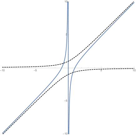
Figure 1: The Boole map $T$ (solid blue lines) and its two inverse branches $\phi_{+},\phi_{-}$ (dashed black lines).

Let us now specialize to local observables $g$ that are even functions of $x$. In view of (7), expression (6) becomes

$$(Pg)(x)=\phi^{\prime}_{+}(x)\,g(\phi_{+}(x))+\phi^{\prime}_{+}(-x)\,g(\phi_{+}(-x)).$$ (8)

This essentially coincides with the Perron-Frobenius operator of the map $\tilde{T}:{\mathbb{R}}^{+}\to{\mathbb{R}}^{+}$ given by

$$\tilde{T}(x):=\left\{\begin{array}[]{ll}\displaystyle x-\frac{1}{x}\,,&\mbox{ if }x\geq 1;\\[12.0pt] \displaystyle\frac{1}{x}-x\,,&\mbox{ if }0<x\leq 1.\end{array}\right.$$ (9)

In fact, $\tilde{T}$ has two inverse branches, $\phi_{0}:[0,+\infty)\to[1,+\infty)$ and $\phi_{1}:[0,+\infty)\to(0,1]$, given by, respectively,

$$\phi_{0}(x) =\phi_{+}(x)=\frac{x}{2}+\xi(x);$$

$$\phi_{1}(x) =\phi_{+}(-x)=-\frac{x}{2}+\xi(x).$$

The graphs of $\tilde{T}$, $\phi_{0}$ and $\phi_{1}$ are depicted in Fig. 2.

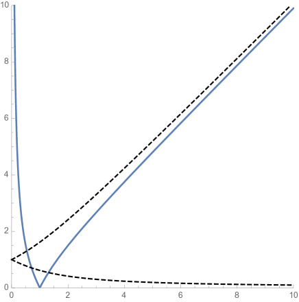
Figure 2: The map $\tilde{T}$ (solid blue lines) and its inverse branches $\phi_{0},\phi_{1}$ (dashed black lines).

Clearly, $\tilde{T}$ preserves the Lebesgue measure on ${\mathbb{R}}^{+}$, which we keep denoting by $m$. The Perron-Frobenius operator $\tilde{P}$ of $\tilde{T}$ acts on functions $\tilde{g}\in L^{1}({\mathbb{R}}^{+},m)$ as

$$(\tilde{P}\tilde{g})(x)=|\phi^{\prime}_{0}(x)|\,\tilde{g}(\phi_{0}(x))+|\phi^{\prime}_{1}(x)|\,\tilde{g}(\phi_{1}(x)).$$

This expression coincides with (8) restricted to $x>0$.

We are thus reduced to studying the transfer operator of the map $\tilde{T}$, which belongs to the class of maps of the half-line studied in [2]. The problem is that in [2] global-local mixing is proved for maps with all increasing branches, and the case of maps with one decreasing branch is only briefly discussed in [2, Remark 2.14].

The following technical lemma is crucial.

Lemma 10.

Let $\tilde{T}$ be defined by (9), with $\tilde{P}$ its associated Perron-Frobenius operator. If

$${\cal F}:=\left\{\tilde{g}\in L^{1}({\mathbb{R}}^{+},m)\,:\,\tilde{g}\in C^{2},\,\tilde{g}>0,\,\tilde{g}^{\prime}<0,\,\tilde{g}^{\prime\prime}+\tilde{g}^{\prime}<0\right\}$$

then $\tilde{P}({\cal F})\subset{\cal F}$.

Lemma 10 is proved in the Appendix, where we first show that its assertion holds for a class of maps with one decreasing and one increasing branch, and then check that $\tilde{T}$ belongs to this class.

The arguments outlined earlier imply the corresponding result for the Boole map $T$:

Corollary 11.

If $g\in L^{1}({\mathbb{R}},m)$ and is $C^{2}$ in ${\mathbb{R}}\setminus\{0\}$, even, positive and such that $g^{\prime}(x)<0$ and $g^{\prime\prime}(x)+g^{\prime}(x)<0$ for all $x>0$, then $Pg$ has the same properties.

We take a $g$ as in Corollary 11 to guarantee that, for all $n$, $P^{n}g$ is even and strictly decreasing on ${\mathbb{R}}^{+}$. In view of Lemma 9, Theorem 8 will be proved once we show that for all global observables $F$,

$$\lim_{n\to\infty}m(F(P^{n}g))=\overline{m}(F)m(g).$$ (10)

We follow the proof of Lemma 4.3 of [2] except for a few twists. First of all, we assume $\overline{m}(F)=0$ and $m(g)=1$, otherwise one can prove (10) for $F_{1}:=F-\overline{m}(F)$ and $g_{1}:=\frac{g}{m(g)}$, and then easily derive it for $F$ and $g$.

Fix $\varepsilon>0$. By definition (2) there exists $\bar{a}>0$ such that

$$\forall a\geq\bar{a},\quad\frac{1}{2a}\left|\int_{-a}^{a}F\,dm\right|\leq\frac{\varepsilon}{2}.$$ (11)

For $x\in{\mathbb{R}}$ and $n\in{\mathbb{N}}$, set

$$\gamma_{n}(x)=\gamma_{n,\bar{a}}(x):=\min\{P^{n}g(\bar{a}),P^{n}g(x)\}.$$

Thus, $\gamma_{n}$ is a positive, even function, flat on $[-\bar{a},\bar{a}]$ and strictly decreasing on $[\bar{a},+\infty)$. It is a local observable because $\|\gamma_{n}\|_{1}\leq\|P^{n}g\|_{1}=\|g\|_{1}=1$.

We defined $\gamma_{n}$ to use it in place of $P^{n}g$ in (10). This can be done to a better and better approximation as $n\to\infty$. The advantage is that, thinking of $\gamma_{n}$ as a density w.r.t. which we integrate $F$, we can “slice” this density into uncountably many horizontal segments, all longer than $2\bar{a}$. By virtue of (11), the integral of $F$ over each segment is very small, thus showing that the original integral is also small.

Let us make this idea precise. Write

$$m(F(P^{n}g))=\int_{-\infty}^{+\infty}F\gamma_{n}\,dm+\int_{-\bar{a}}^{\bar{a}}F(P^{n}g-\gamma_{n})\,dm=:\mathcal{I}_{1}+\mathcal{I}_{2}.$$ (12)

We first consider $\mathcal{I}_{2}$. Since $P^{n}g\geq\gamma_{n}>0$ we have

$$0\leq\int_{-\bar{a}}^{\bar{a}}(P^{n}g-\gamma_{n})\,dm\leq\int_{-\bar{a}}^{\bar{a}}P^{n}g\,dm=m\!\left((1_{[-\bar{a},\bar{a}]}\circ T^{n})g\right),$$

where $1_{[-\bar{a},\bar{a}]}$ is the indicator function of $[-\bar{a},\bar{a}]$. The fact that $T$ is of zero-type (see Corollary 3 and following paragraph) implies that the rightmost term above vanishes as $n\to\infty$. Thus, for all sufficiently large $n$,

$$|\mathcal{I}_{2}|\leq\|F\|_{\infty}\int_{-a}^{a}(P^{n}g-\gamma_{n})\,dm\leq\frac{\varepsilon}{2}.$$ (13)

Now for $\mathcal{I}_{1}$. For $0<r<\max\gamma_{n}=\gamma_{n}(\bar{a})$, let $a(r)$ be uniquely defined by

$$a(r)>\bar{a},\quad\gamma_{n}(a(r))=r.$$

In other words, $a(r)=\left(\gamma_{n}|_{(\bar{a},+\infty)}\right)^{-1}(r)$. We rewrite $\mathcal{I}_{1}$ as

$$\mathcal{I}_{1}=\int_{-\infty}^{+\infty}\!F(x)\left(\int_{0}^{\gamma_{n}(x)}\!\!\ dr\right)dx=\int_{0}^{\gamma_{n}(\bar{a})}\!\left(\int_{-a(r)}^{a(r)}\!F(x)\,dx\right)dr,$$

where we have used Fubini’s Theorem. Using (11) with $a:=a(r)$, we estimate the above as follows:

$$\begin{split}|\mathcal{I}_{1}|&\leq\int_{0}^{\gamma_{n}(\bar{a})}\left|\int_{-a(r)}^{a(r)}\!F(x)\,dx\right|dr\leq\frac{\varepsilon}{2}\int_{0}^{\gamma_{n}(\bar{a})}\!2a(r)\,dr\\ &=\frac{\varepsilon}{2}\,m(\gamma_{n})\leq\frac{\varepsilon}{2},\end{split}$$

because $m(\gamma_{n})=\|\gamma_{n}\|_{1}\leq 1$. The above estimate holds uniformly in $n$. Together with (12) and (13), it implies (10) for the case $\overline{m}(F)=0$ and $m(g)=1$. As already discussed, this is enough to prove Theorem 8. ∎

3 Application

We conclude our exposition by presenting a more sophisticated application of global-local mixing than previously discussed (in the paragraphs after Definition 6). It has to do with the stochastic properties of our map, that is, with the interpretation of observables as random variables w.r.t. a random choice of the initial condition. The interested reader will find more details in Section 3.2 of [2].

Definition 12.

Let $F_{n}$ be a sequence of measurable functions ${\mathbb{R}}\to{\mathbb{R}}$ and $X$ a random variable on some probability space $(\Omega,{\mathbb{P}})$. We say that $F_{n}$ converges to $X$ in strong distributional sense, as $n\to\infty$, if for all probability measures $\nu\ll m$ the distribution of $F_{n}$ w.r.t. $\nu$ converges to that of $X$.

Proposition 13.

Let $T$ be the Boole map and $F:{\mathbb{R}}\to{\mathbb{R}}$ a measurable function such that $\overline{m}(e^{i\theta F})$ exists for all $\theta\in{\mathbb{R}}$. Then $F\circ T^{n}$ converges in strong distributional sense, as $n\to\infty$, to the random variable $X$ with characteristic function $\varphi_{X}(\theta):=\overline{m}(e^{i\theta F})$.

Proof.

Given a probability measure $\nu\ll m$, let $g$ denote its Radon-Nikodym derivative $\frac{d\nu}{dm}$. For all $\theta\in{\mathbb{R}}$, $e^{i\theta F}$ is a global observable by hypothesis (observe that $F$ takes values in ${\mathbb{R}}$). Thus, by global-local mixing,

$$\lim_{n\to\infty}\nu(e^{i\theta F\circ T^{n}})=\lim_{n\to\infty}m((e^{i\theta F\circ T^{n}})g)=\overline{m}(e^{i\theta F})=\varphi_{X}(\theta).$$

Pointwise convergence of the characteristic function is equivalent to convergence in distribution. ∎

We illustrate this property by means of an example similar to the one presented after Definition 6. Set $F(x):=\{x\}$, where $\{\cdot\}$ denotes the fractional part of a real number. It is very easy to verify that $\overline{m}(e^{i\theta F})=\int_{0}^{1}e^{i\theta x}\,dx$, for all $\theta$. Therefore, Proposition 13 implies that for a random initial condition $x$, w.r.t. any law $\nu\ll m$, the fractional part of $T^{n}(x)$ tends to be uniformly distributed in $[0,1)$, as $n\to\infty$.

Adding a small hypothesis on $F$ gives a result that is peculiar to maps with neutral fixed points in whose neighborhoods lies “most” of the infinite invariant measure. This is the case for the Boole map too.

Definition 14.

We say that $F:{\mathbb{R}}\to{\mathbb{R}}$ is uniformly continuous at infinity if, for every $\varepsilon>0$, there exist $\delta,Q>0$ such that

$$\forall x,y\in{\mathbb{R}}\setminus(-Q,Q)\mbox{ with }|x-y|\leq\delta,\quad|F(x)-F(y)|\leq\varepsilon.$$

Proposition 15.

In addition to the hypotheses of Proposition 13, suppose that $F$ is bounded and uniformly continuous at infinity. Also, for $k\in{\mathbb{Z}}^{+}$, denote by

$$\mathcal{A}_{k}F:=\frac{1}{k}\sum_{j=0}^{k-1}F\circ T^{j}$$

the partial Birkhoff average of $F$. Then:

• For $k$ fixed and $n\to\infty$, $\mathcal{A}_{k}F\circ T^{n}$ converges in strong distributional sense to the random variable $X$ defined in the statement of Proposition 13.

• There exists a diverging subsequence $(k_{n})$ such that, as $n\to\infty$, $\mathcal{A}_{k_{n}}F\circ T^{n}$ converges in strong distributional sense to $X$.

The significance of Proposition 15 is that, for the Boole map, the asymptotic distribution of an observable is the same as that of any of its partial time averages, at least for a large class of global observables. This phenomenon cannot occur for mixing maps preserving a finite measure, cf. [2, Section 3.2]. Proposition 15 is proved almost exactly as Proposition 3.5 of [2]. The fact that the latter refers to maps ${\mathbb{R}}^{+}\to{\mathbb{R}}^{+}$ and is formulated with a slightly stronger assumption on $F$ plays no substantial role.

Coming back to the example $F(x)=\{x\}$, one may observe that $F$ is not uniformly continuous at infinity. But we can define a very similar observable which is. For $x\in{\mathbb{R}}$, let $\lfloor x\rfloor$ denote the maximum integer not exceeding $x$; for $x\geq 0$, $\lfloor x\rfloor$ is the integer part of $x$, whence $x-\lfloor x\rfloor$ is its fractional part. Set

$$F_{1}(x):=\left\{\begin{array}[]{cl}x-\lfloor x\rfloor\,,&\mbox{ if $\lfloor x\rfloor$ is even};\\[2.0pt] 1-x+\lfloor x\rfloor\,,&\mbox{ if $\lfloor x\rfloor$ is odd}.\end{array}\right.$$

As in the previous example, $F_{1}\circ T^{n}$ tends to be uniformly distributed on $[0,1]$, when $n\to\infty$. By Proposition 15, so do $\mathcal{A}_{k}F_{1}\circ T^{n}$ and $\mathcal{A}_{k_{n}}F_{1}\circ T^{n}$, for a certain subsequence $(k_{n})$.

Remark 16.

A question that may be of interest is this: what random variables $X$ can be strong distributional limits of $F\circ T^{n}$, for some $F$? The answer is all random variables. In fact, given a variable $X$ on a probability space $(\Omega,{\mathbb{P}})$, let $\Phi(y):={\mathbb{P}}(X\leq y)$ denote its distribution function and

$$\Phi^{-1}(x):=\inf\,\{y\in{\mathbb{R}}\,:\,\Phi(y)>x\}$$

the right-continuous generalized inverse of $\Phi$. Here $x\in[0,1)$. It is well-known that, calling $U$ the uniform random variable on $[0,1]$, $\Phi^{-1}\circ U=X$ (in the sense of distributions). In other words, $\phi_{X}(\theta)=\int_{0}^{1}e^{i\theta\Phi^{-1}(x)}\,dx$. Therefore, if $F(x):=\Phi^{-1}(x-\lfloor x\rfloor)$ is the periodization of $\Phi^{-1}$, then clearly

$$\overline{m}(e^{i\theta F})=\int_{0}^{1}e^{i\theta\Phi^{-1}(x)}\,dx=\phi_{X}(\theta)$$

and Proposition 13 applies.

But $F$ may not be bounded and is surely not continuous — for a periodic function, continuity is the same as uniform continuity at infinity — so, if the question is: for what variables $X$ do the assertions of Proposition 15 hold?, the answer is: at least all variables which take values densely in an interval $[a,b]$ (this means that ${\mathbb{P}}(X\in[a,b])=1$ and ${\mathbb{P}}(X\in[c,d])>0$, for all $[c,d]\subseteq[a,b]$). In fact, for any such variable, $\Phi^{-1}$ takes values in $[a,b]$ and is continuous. Therefore, the function

$$F_{1}(x):=\left\{\begin{array}[]{cl}\Phi^{-1}(x-\lfloor x\rfloor)\,,&\mbox{ if $\lfloor x\rfloor$ is even};\\[2.0pt] \Phi^{-1}(1-x+\lfloor x\rfloor)\,,&\mbox{ if $\lfloor x\rfloor$ is odd}\end{array}\right.$$

is bounded, 2-periodic, continuous and such that $\overline{m}(e^{i\theta F_{1}})=\phi_{X}(\theta)$. It thus satisfies the hypotheses of Proposition 15.

Appendix A Appendix: Proof of Lemma 10

We consider a generic map $S:{\mathbb{R}}^{+}\to{\mathbb{R}}^{+}$, which is Markov and piecewise $C^{3}$ with respect to the partition $I_{0}:=[a,+\infty)$, $I_{1}:=(0,a]$. It also satisfies the following hypotheses (H1)-(H4).

1. $S(I_{0})=S(I_{1})={\mathbb{R}}_{0}^{+}$;

2. $\forall x\in I_{0}$, $S^{\prime}(x)>1$; $S^{\prime}(x)\to 1$ as $x\to\infty$; $\forall x\in I_{1}$, $S^{\prime}(x)<-1$;

3. $S$ preserves the Lebesgue measure $m$.

Denoting $\phi_{j}:=\left(S|_{I_{j}}\right)^{-1}$, for $j\in\{0,1\}$, we rewrite (H2) as follows

• • $\phi_{0}(0)=a$; $\forall x\in{\mathbb{R}}_{0}^{+}$, $0<\phi^{\prime}_{0}(x)<1$; $\phi^{\prime}_{0}(x)\to 1$ as $x\to\infty$;

  • $\phi_{1}(0)=a$; $\forall x\in{\mathbb{R}}_{0}^{+}$, $-1<\phi^{\prime}_{1}(x)<0$.

Let $L:L^{1}({\mathbb{R}}^{+},m)\to L^{1}({\mathbb{R}}^{+},m)$ be the Perron-Frobenius operator associated to $S$, i.e., the transfer operator relative to the Lebesgue measure $m$. In formula:

$$(Lg)(x)=\phi_{0}^{\prime}(x)\,g(\phi_{0}(x))-\phi_{1}^{\prime}(x)\,g(\phi_{1}(x)).$$

If we let $L$ act on $1$, the function identically equal to 1 on ${\mathbb{R}}_{0}^{+}$, noting that strictly speaking $1$ does not belong to $L^{1}$, we observe that (H3) is equivalent to $L1=1$, or

1. $\forall x\in{\mathbb{R}}_{0}^{+}$, $\phi_{0}^{\prime}(x)-\phi_{1}^{\prime}(x)=1$.

Notice that (H3) implies that $\phi^{\prime\prime}_{0}(x)=\phi^{\prime\prime}_{1}(x)$ and $\phi^{\prime\prime\prime}_{0}(x)=\phi^{\prime\prime\prime}_{1}(x)$.

We further assume that

• • $\forall x\in{\mathbb{R}}^{+}$, $1+2\phi^{\prime}_{1}(x)>0$;

  • $\forall x\in{\mathbb{R}}^{+}$, $\phi^{\prime\prime}_{1}(x)-(\phi^{\prime}_{1}(x))^{2}>0$;

  • for all $x\in{\mathbb{R}}^{+}$ one of the following is satisfied:

    • $\phi^{\prime\prime\prime}_{1}(x)+\phi^{\prime\prime}_{1}(x)>0$ and $3\,\phi^{\prime\prime}_{1}(x)-(\phi^{\prime}_{1}(x))^{2}+\phi^{\prime}_{1}(x)>0$

    • $\phi^{\prime\prime\prime}_{1}(x)+\phi^{\prime\prime}_{1}(x)-(\phi^{\prime}_{1}(x))^{2}>0$.

Observe that condition (H4)(i) is equivalent to $\phi_{1}^{\prime}(x)>-1/2$ and thus supersedes one of the inequalities of (H2)(ii). We prefer to leave the latter as it is because the meaning of (H2) is that $S$ has one decreasing and one increasing branch, both expanding.

Theorem 17.

Let $S$ be a piecewise $C^{3}$ map w.r.t. a partition $I_{0}=[a,+\infty)$, $I_{1}=(0,a]$ and assume that $S$ satisfies (H1)-(H4). Setting

$$\mathcal{F}:=\left\{g:{\mathbb{R}}^{+}\to{\mathbb{R}}\,:\,g\in C^{2},\,g>0,\,g^{\prime}<0,\,g^{\prime\prime}+g^{\prime}<0\right\}$$

we have $L(\mathcal{F})\subset\mathcal{F}$.

Proof.

The $C^{2}$-regularity and the positivity of $Lg$ for any $g\in\mathcal{F}$ follow easily from the definition of the transfer operator. To verify the last two conditions we first write, using (H3),

$$\begin{split}(Lg)^{\prime}(x)&=\phi^{\prime\prime}_{0}(x)\,g(\phi_{0}(x))-\phi^{\prime\prime}_{1}(x)\,g(\phi_{1}(x))\\[6.0pt] &\qquad+(\phi^{\prime}_{0}(x))^{2}\,g^{\prime}(\phi_{0}(x))-(\phi^{\prime}_{1}(x))^{2}\,g^{\prime}(\phi_{1}(x))\\[2.0pt] &=\phi^{\prime\prime}_{1}(x)\int_{\phi_{1}(x)}^{\phi_{0}(x)}\!\!\ g^{\prime}(t)\,dt+g^{\prime}(\phi_{0}(x))\,(1+2\phi^{\prime}_{1}(x))\\ &\qquad+(\phi^{\prime}_{1}(x))^{2}\,\Big{[}g^{\prime}(\phi_{0}(x))-g^{\prime}(\phi_{1}(x))\Big{]}\\ &=\phi^{\prime\prime}_{1}(x)\int_{\phi_{1}(x)}^{\phi_{0}(x)}\!\!g^{\prime}(t)\,dt+(\phi^{\prime}_{1}(x))^{2}\int_{\phi_{1}(x)}^{\phi_{0}(x)}\!g^{\prime\prime}(t)\,dt\\[2.0pt] &\qquad+g^{\prime}(\phi_{0}(x))\,(1+2\phi^{\prime}_{1}(x))\end{split}$$ (14)

and

$$\begin{split}(Lg)^{\prime\prime}(x)&=\phi^{\prime\prime\prime}_{1}(x)\int_{\phi_{1}(x)}^{\phi_{0}(x)}\!\!g^{\prime}(t)\,dt+3\,\phi^{\prime\prime}_{1}(x)\,\phi^{\prime}_{0}(x)\,g^{\prime}(\phi_{0}(x))\\[2.0pt] &\qquad-3\,\phi^{\prime\prime}_{1}(x)\,\phi^{\prime}_{1}(x)\,g^{\prime}(\phi_{1}(x))+(\phi^{\prime}_{0}(x))^{3}g^{\prime\prime}(\phi_{0}(x))\\[6.0pt] &\qquad-(\phi^{\prime}_{1}(x))^{3}\,g^{\prime\prime}(\phi_{1}(x)).\end{split}$$ (15)

Now we prove that $(Lg)^{\prime}(x)<0$ for all $x\in{\mathbb{R}}^{+}$. From (14), since $g^{\prime\prime}+g^{\prime}<0$, we have

$$(Lg)^{\prime}(x)<\left[\phi^{\prime\prime}_{1}(x)-(\phi^{\prime}_{1}(x))^{2}\right]\int_{\phi_{1}(x)}^{\phi_{0}(x)}\!\!g^{\prime}(t)\,dt+g^{\prime}(\phi_{0}(x))\,(1+2\phi^{\prime}_{1}(x)).$$

The claim follows from (H4)(i)-(ii) and the hypothesis $g^{\prime}<0$.

To show that $(Lg)^{\prime\prime}+(Lg)^{\prime}<0$ we begin from (15) and, using different arguments, we obtain the result for all $x\in{\mathbb{R}}^{+}$ for which (H4)(iii) (a) or (b) are satisfied. In the case (a), we use $g^{\prime\prime}+g^{\prime}<0$ to write

$$\begin{split}&(Lg)^{\prime\prime}(x)+(Lg)^{\prime}(x)=\left[\phi^{\prime\prime\prime}_{1}(x)+\phi^{\prime\prime}_{1}(x)\right]\int_{\phi_{1}(x)}^{\phi_{0}(x)}\!\!g^{\prime}(t)\,dt\\ &\qquad\qquad+(\phi^{\prime}_{0}(x))^{3}g^{\prime\prime}(\phi_{0}(x))-(\phi^{\prime}_{1}(x))^{3}g^{\prime\prime}(\phi_{1}(x))\\[6.0pt] &\qquad\qquad+\left[3\,\phi^{\prime\prime}_{1}(x)\,\phi^{\prime}_{0}(x)+(\phi^{\prime}_{0}(x))^{2}\right]g^{\prime}(\phi_{0}(x))\\[6.0pt] &\qquad\qquad-\left[3\,\phi^{\prime\prime}_{1}(x)\,\phi^{\prime}_{1}(x)+(\phi^{\prime}_{1}(x))^{2}\right]g^{\prime}(\phi_{1}(x))\\ &\qquad<\left[\phi^{\prime\prime\prime}_{1}(x)+\phi^{\prime\prime}_{1}(x)\right]\int_{\phi_{1}(x)}^{\phi_{0}(x)}\!\!\ g^{\prime}(t)\,dt\\ &\qquad\qquad+\left[3\,\phi^{\prime\prime}_{1}(x)\,\phi^{\prime}_{0}(x)+(\phi^{\prime}_{0}(x))^{2}-(\phi^{\prime}_{0}(x))^{3}\right]g^{\prime}(\phi_{0}(x))\\[6.0pt] &\qquad\qquad+\left[-3\,\phi^{\prime\prime}_{1}(x)\,\phi^{\prime}_{1}(x)-(\phi^{\prime}_{1}(x))^{2}+(\phi^{\prime}_{1}(x))^{3}\right]g^{\prime}(\phi_{1}(x)).\end{split}$$ (16)

Let $x$ satisfy (H4)(iii)(a). We argue that all three terms in the last expression are negative. The first term is negative by the first condition of (H4)(iii)(a) and the fact that $g^{\prime}<0$. The third term is negative by the second condition of (H4)(iii)(a) and the inequalities $\phi^{\prime}_{1}<0$ and $g^{\prime}<0$. For the second term we use (H3) to get

$$3\,\phi^{\prime\prime}_{1}(x)\,\phi^{\prime}_{0}(x)+(\phi^{\prime}_{0}(x))^{2}-(\phi^{\prime}_{0}(x))^{3}=\phi^{\prime}_{0}(x)\left[3\,\phi^{\prime\prime}_{1}(x)-(\phi^{\prime}_{1}(x))^{2}-\phi^{\prime}_{1}(x)\right].$$

Since $\phi^{\prime}_{0}>0$ and $\phi^{\prime}_{1}<0$, using the second condition of (H4)(iii)(a), we obtain

$$3\,\phi^{\prime\prime}_{1}(x)\,\phi^{\prime}_{0}(x)+(\phi^{\prime}_{0}(x))^{2}-(\phi^{\prime}_{0}(x))^{3}>-2\,\phi^{\prime}_{0}(x)\,\phi^{\prime}_{1}(x)>0.$$

Together with $g^{\prime}<0$, this shows that the second term of (16) is negative. In conclusion, $(Lg)^{\prime\prime}(x)+(Lg)^{\prime}(x)<0$.

We now show that we obtain the same conclusion for all $x$ for which (H4)(iii)(b) is satisfied. Adding to (15) the last expression of (14), we have

$$(Lg)^{\prime\prime}(x)+(Lg)^{\prime}(x)=\left[\phi^{\prime\prime\prime}_{1}(x)+\phi^{\prime\prime}_{1}(x)\right]\int_{\phi_{1}(x)}^{\phi_{0}(x)}\!\!g^{\prime}(t)\,dt$$

$$\qquad\qquad+(\phi^{\prime}_{0}(x))^{3}g^{\prime\prime}(\phi_{0}(x))-(\phi^{\prime}_{1}(x))^{3}g^{\prime\prime}(\phi_{1}(x))$$

$$\qquad\qquad+3\,\phi^{\prime\prime}_{1}(x)\,\phi^{\prime}_{0}(x)\,g^{\prime}(\phi_{0}(x))-3\,\phi^{\prime\prime}_{1}(x)\,\phi^{\prime}_{1}(x)\,g^{\prime}(\phi_{1}(x))$$

$$\qquad\qquad+(\phi^{\prime}_{1}(x))^{2}\int_{\phi_{1}(x)}^{\phi_{0}(x)}\!\!\ g^{\prime\prime}(t)\,dt+g^{\prime}(\phi_{0}(x))\,(1+2\phi^{\prime}_{1}(x)).$$

Using again the hypothesis $g^{\prime\prime}+g^{\prime}<0$ we can write

$$(Lg)^{\prime\prime}(x)+(Lg)^{\prime}(x)<\left[\phi^{\prime\prime\prime}_{1}(x)+\phi^{\prime\prime}_{1}(x)-(\phi^{\prime}_{1}(x))^{2}\right]\int_{\phi_{1}(x)}^{\phi_{0}(x)}\!\!\ g^{\prime}(t)\,dt$$

$$\qquad\qquad+\left[-3\,\phi^{\prime\prime}_{1}(x)\,\phi^{\prime}_{1}(x)+(\phi^{\prime}_{1}(x))^{3}\right]g^{\prime}(\phi_{1}(x))$$

$$\qquad\qquad+\left[3\,\phi^{\prime\prime}_{1}(x)\,\phi^{\prime}_{0}(x)+1+2\phi^{\prime}_{1}(x)-(\phi^{\prime}_{0}(x))^{3}\right]g^{\prime}(\phi_{0}(x)).$$

The first term on the above right hand side is negative by (H4)(iii)(b) and the inequality $g^{\prime}<0$. The second term is negative because $\phi^{\prime}_{1}<0$, $g^{\prime}<0$ and, by (H4)(ii), $3\phi^{\prime\prime}_{1}(x)-(\phi^{\prime}_{1}(x))^{2}>2(\phi^{\prime}_{1}(x))^{2}>0$. As for the third term we use once more that $g^{\prime}<0$. Furthermore, via (H3),

$$3\,\phi^{\prime\prime}_{1}(x)\,\phi^{\prime}_{0}(x)+1+2\phi^{\prime}_{1}(x)-(\phi^{\prime}_{0}(x))^{3}$$

$$\quad=\phi^{\prime}_{0}(x)\left[3\,\phi^{\prime\prime}_{1}(x)-1-2\phi^{\prime}_{1}(x)-(\phi^{\prime}_{1}(x))^{2}\right]+1+2\phi^{\prime}_{1}(x)$$

$$\quad=\phi^{\prime}_{0}(x)\left[3\,\phi^{\prime\prime}_{1}(x)-(\phi^{\prime}_{1}(x))^{2}\right]+(1+2\phi^{\prime}_{1}(x))\,(1-\phi^{\prime}_{0}(x)).$$

The last expression above is positive because of the conditions (H4)(i)-(ii) and the fact that $\phi^{\prime}_{0}\in(0,1)$. This concludes the proof that $(Lg)^{\prime\prime}(x)+(Lg)^{\prime}(x)<0$ for all $x$ that satisfy (H4)(iii)(b). ∎

In order to prove Lemma 10 it remains to verify that the map $\tilde{T}$ defined in (9) satisfies the assumptions of Theorem 17.

First of all, $\tilde{T}$ is piecewise $C^{3}$ with respect to the partition $I_{0}=[1,+\infty)$ and $I_{1}=(0,1]$ and (H1) is evidently satisfied. Moreover we have

$$\phi_{0}(x)=\frac{x+\sqrt{x^{2}+4}}{2},\qquad\phi_{1}(x)=\frac{-x+\sqrt{x^{2}+4}}{2},$$

whence

$$\phi^{\prime}_{0}(x)=\frac{1}{2}+\frac{x}{2\,\sqrt{x^{2}+4}},\quad \quad\phi^{\prime}_{1}(x)=-\frac{1}{2}+\frac{x}{2\,\sqrt{x^{2}+4}},$$

$$\phi^{\prime\prime}_{0}(x)=\phi^{\prime\prime}_{1}(x) =\frac{2}{(x^{2}+4)^{\frac{3}{2}}},$$

$$\phi^{\prime\prime\prime}_{0}(x)=\phi^{\prime\prime\prime}_{1}(x) =-\frac{6\,x}{(x^{2}+4)^{\frac{5}{2}}}.$$

From these expressions we can immediately verify (H2) and (H3). Moreover

$$1+2\phi^{\prime}_{1}(x)=\frac{x}{\sqrt{x^{2}+4}}$$

gives (H4)(i). Now let us compute

$$\phi^{\prime\prime}_{1}(x)-(\phi^{\prime}_{1}(x))^{2}=-\frac{1}{4\,(x^{2}+4)^{\frac{3}{2}}}\left[\sqrt{x^{2}+4}\left(\sqrt{x^{2}+4}-x\right)^{2}\!-8\right].$$

One easily checks that

$$\frac{d}{dx}\left[\sqrt{x^{2}+4}\left(\sqrt{x^{2}+4}-x\right)^{2}\!-8\right]$$

$$\qquad=\left(3x\,\sqrt{x^{2}+4}-3x^{2}-8\right)\frac{\sqrt{x^{2}+4}-x}{\sqrt{x^{2}+4}}<0,$$

for $x>0$. Hence, for all $x>0$,

$$\sqrt{x^{2}+4}\left(\sqrt{x^{2}+4}-x\right)^{2}\!-8<0,$$

which implies (H4)(ii).

In order to check assumption (H4)(iii), define:

$$A_{1} :=\left\{x\in{\mathbb{R}}^{+}\,:\,\phi^{\prime\prime\prime}_{1}(x)+\phi^{\prime\prime}_{1}(x)>0\right\};$$

$$A_{2} :=\left\{x\in{\mathbb{R}}^{+}\,:\,3\,\phi^{\prime\prime}_{1}(x)-(\phi^{\prime}_{1}(x))^{2}+\phi^{\prime}_{1}(x)>0\right\};$$

$$B :=\left\{x\in{\mathbb{R}}^{+}\,:\,\phi^{\prime\prime\prime}_{1}(x)+\phi^{\prime\prime}_{1}(x)-(\phi^{\prime}_{1}(x))^{2}>0\right\}.$$

Clearly (H4)(iii) is satisfied if and only if

$$\left(A_{1}\cap A_{2}\right)\cup B={\mathbb{R}}^{+}.$$

Also notice that it follows immediately from the definitions that $B\subseteq A_{1}$. Let us determine $A_{1},A_{2}$ and $B$ in our case.

First of all $A_{1}={\mathbb{R}}^{+}$ because

$$\phi^{\prime\prime\prime}_{1}(x)+\phi^{\prime\prime}_{1}(x)=\frac{2\,(x^{2}-3x+4)}{(x^{2}+4)^{\frac{5}{2}}}.$$

As for $A_{2}$,

$$3\,\phi^{\prime\prime}_{1}(x)-(\phi^{\prime}_{1}(x))^{2}+\phi^{\prime}_{1}(x)=\frac{(x^{2}+4)^{\frac{3}{2}}-\sqrt{x^{2}+4}\left(2\,\sqrt{x^{2}+4}-x\right)^{2}\!+24}{4\,(x^{2}+4)^{\frac{3}{2}}}.$$

Elementary calculus shows that the function in the numerator vanishes at $x=0$, is increasing up to $x=\sqrt{\frac{7\sqrt{33}-9}{12}}$ and is decreasing afterwards. Evaluation at integers proves that the numerator is positive at least up to $x=5$, hence $(0,5)\subset A_{2}$. (Numerical computations give the approximate result $A_{2}=(0,x_{1})$, with $x_{1}\simeq 5.25166$.) Since $A_{1}={\mathbb{R}}^{+}$ we conclude that

$$(0,5)\subset A_{1}\cap A_{2}.$$ (17)

We now study $B$.

$$\phi^{\prime\prime\prime}_{1}(x)+\phi^{\prime\prime}_{1}(x)-(\phi^{\prime}_{1}(x))^{2}$$

$$\qquad=\frac{8(x^{2}+4)-24x-(x^{2}+4)^{\frac{3}{2}}\left(\sqrt{x^{2}+4}-x\right)^{2}}{4\,(x^{2}+4)^{\frac{5}{2}}}$$

$$\qquad=\frac{(x^{5}+8x^{3}+4x^{2}+4x+16)-\sqrt{x^{2}+4}\,(x^{4}+6x^{2}+8)}{2\,(x^{2}+4)^{\frac{5}{2}}}.$$

It follows that

$$\lim_{x\to+\infty}\left[\phi^{\prime\prime\prime}_{1}(x)+\phi^{\prime\prime}_{1}(x)-(\phi^{\prime}_{1}(x))^{2}\right]=+\infty$$

and that, for $x\in{\mathbb{R}}^{+}$, the zeroes of $\phi^{\prime\prime\prime}_{1}(x)+\phi^{\prime\prime}_{1}(x)-(\phi^{\prime}_{1}(x))^{2}$ are the same as the roots of the polynomial

$$p(x):=2x^{6}-7x^{5}+24x^{4}-56x^{3}+72x^{2}-76x+32.$$

By applying synthetic substitution, we obtain

$$p(x)=(x-4)\,(2x^{5}+x^{4}+28x^{3}+56x^{2}+296x+1108)+4464,$$

which proves that the largest positive root of $p(x)$ is smaller than 4. This implies that

$$(4,+\infty)\subset B.$$ (18)

(Numerical computations show that $B=(0,x_{2})\cup(x_{3},+\infty)$, with $x_{2}\simeq 0.690123$ and $x_{3}\simeq 1.93158$.)

Inclusions (17) and (18) show that $\left(A_{1}\cap A_{2}\right)\cup B={\mathbb{R}}^{+}$, which gives (H4)(iii) and ends the proof of Lemma 10. ∎

References

• [1] J. Aaronson, “An Introduction to Infinite Ergodic Theory”, Mathematical Surveys and Monographs, vol.‘50, American Mathematical Society, 1997
• [2] C. Bonanno, P. Giulietti, M. Lenci, Infinite mixing for one-dimensional maps with an indifferent fixed point, arXiv:1708.09369 [math.DS]
• [3] G. Boole, On the comparison of transcendence, with certain applications to the theory of definite integrals, Philos. Trans. R. Soc. Lond 147 (1857), 745–803
• [4] A. I. Danilenko, C. E. Silva, Ergodic Theory: nonsingular transformations, in: R. E. Meyers (ed.), Encyclopedia of Complexity and Systems Science, pp. 3055–3083, Springer, 2009
• [5] A. B. Hajian and S. Kakutani, Weakly wandering sets and invariant measures, Trans. Amer. Math. Soc. 110 (1964), 136–151
• [6] M. Lenci, On infinite-volume mixing, Comm. Math. Phys. 298 (2010), no. 2, 485–514
• [7] M. Lenci, Exactness, k-property and infinite mixing, Publ. Mat. Urug. 14 (2013), 159–170
• [8] M. Lenci, Uniformly expanding Markov maps of the real line: exactness and infinite mixing, Discrete Contin. Dyn. Syst. 37 (2017), no. 7, 3867–3903
• [9] M. Lin, Mixing for Markov operators, Z. Wahrscheinlichkeitstheorie und Verw. Gebiete 19 (1971), 231–242
• [10] R. Zweimüller, Surrey Notes on Infinite Ergodic Theory, 2009, available at http://mat.univie.ac.at/~zweimueller/MyPub/SurreyNotes.pdf