Approximate Message Passing for
Underdetermined Audio Source Separation

Abstract

Approximate message passing (AMP) algorithms have shown great promise in sparse signal reconstruction due to their low computational requirements and fast convergence to an exact solution. Moreover, they provide a probabilistic framework that is often more intuitive than alternatives such as convex optimisation. In this paper, AMP is used for audio source separation from underdetermined instantaneous mixtures. In the time-frequency domain, it is typical to assume a priori that the sources are sparse, so we solve the corresponding sparse linear inverse problem using AMP. We present a block-based approach that uses AMP to process multiple time-frequency points simultaneously. Two algorithms known as AMP and vector AMP (VAMP) are evaluated in particular. Results show that they are promising in terms of artefact suppression.

1 Introduction

Source separation is a problem in which an unknown set of source signals must be estimated from a known set of mixture signals. For audio separation, this corresponds to segregating sounds produced by distinct entities, such as different human speakers or musical instruments. A common formulation of the problem is the linear instantaneous model given by

$$\mathbf{y}(t)=\mathbf{A}\mathbf{x}(t)+\mathbf{w}(t),$$ (1)

where $\mathbf{y}(t)\in\mathbb{R}^{M}$ denotes the mixtures, $\mathbf{x}(t)\in\mathbb{R}^{N}$ denotes the sources, $\mathbf{A}\in\mathbb{R}^{M\times N}$ is the mixing matrix and $\mathbf{w}(t)\in\mathbb{R}^{N}$ is noise. The model assumes the mixtures at each instance of $t$ are instantaneous (memory-less), which means reverberation effects and time delays are ignored. Although the notation suggests the signals are in the time domain, it can also apply to signals in the time-frequency domain, with $t$ referring to a time-frequency point. This will be described in Section 3.

When $N>M$, the problem is underdetermined, and no unique solution exists. To find a unique solution, the problem must be regularised by introducing a constraint, which often corresponds to a property of the solution known a priori. By modelling this prior knowledge as a probability distribution, $p(\mathbf{x})$, the sources can be inferred using a suitable estimator. For example, the maximum a posteriori (MAP) estimate is

$$\mathbf{\hat{x}}=\operatorname*{arg\!\,max}_{\mathbf{x}\in\mathbb{R}^{N}}p(\mathbf{x}|\mathbf{y}),$$ (2)

where $p(\mathbf{x}|\mathbf{y})$ is the posterior distribution. Assuming $\mathbf{x}$ and $\mathbf{w}$ are independent of each other and contain i.i.d. components,

$$p(\mathbf{x}|\mathbf{y})\propto\prod_{i=1}^{M}p(w_{i}-(\mathbf{A}\mathbf{x})_{i})\prod_{j=1}^{N}p(x_{j}).$$ (3)

The choice of the prior, $p(\mathbf{x})$, is important, as it affects the separation performance of the system. In the time-frequency domain, it has been shown experimentally that sources tend to be sparse [1, 2, 3], so choosing a prior that enforces sparsity is an effective approach. As for the choice of $p(\mathbf{w})$, we adopt the standard assumption that $p(w_{i})\sim\mathcal{N}(0,{\gamma_{\omega}}^{-1})$, $i=1,...,M$, where $\gamma_{\omega}$ is the precision (inverse of variance) of the noise.

Using this probabilistic framework, we investigate the use of approximate message passing (AMP) algorithms for audio separation. The original AMP algorithm [4] was proposed as an alternative for $L_{1}$ regularisation, and was formulated as an approximation to belief propagation. It has been shown to converge to an exact solution when $N,M\to\infty$ and when the components of $\mathbf{A}$ follow a sub-Gaussian distribution with zero mean [5]. Its fast convergence and low computational complexity are reasons why it is promising. Since then, AMP algorithms have been developed for arbitrary priors [6], noise distributions [7] and arbitrary $\mathbf{A}$ [8, 9, 10, 11, 12].

It must be emphasised that AMP is only accurate for large $M$ and $N$, but the instantaneous formulation given by (1) results in small dimensions in practice. For example, a stereo signal containing three sources means that $M=2,N=3$. To overcome this, we propose to take a block-based approach in which blocks of samples are considered together rather than individually. This results in the dimensions of the problem being proportional to the block size.

The paper is organised as follows. In Section 2, the AMP algorithms used to implement audio source separation are outlined. In Section 3, we describe how the overall system is implemented, including the time-frequency representation used and the choice of parameters for the AMP algorithms. In Section 4, the system is evaluated and results are presented. Finally, we summarise and suggest future work in Section 5.

2 AMP Algorithms

Two algorithms are investigated in particular. The first is listed in Algorithm 1 and is simply dubbed AMP. It is based on the original algorithm, but allows an arbitrary prior and supports damping [9]. The purpose of damping is to make the algorithm robust to instances of $\mathbf{A}$ that deviate from a zero-mean sub-Gaussian distribution, and is controlled by the damping factor, $\theta\in(0,1]$, where $\theta=1$ means no damping. $\mathbf{g}_{1}(\cdot)$ is a scalar function that estimates the real solution based on the given noisy solution, $\mathbf{r}_{t}$. For MAP estimation, its definition is given by (2). $\mathbf{g}^{\prime}_{1}(\cdot)$ is the derivative of $\mathbf{g}_{1}(\cdot)$ and $\langle\mathbf{v}\rangle$ is the arithmetic mean of the components of vector $\mathbf{v}$.

The second algorithm is described in Algorithm 2 and is known as vector AMP (VAMP) [12]. $\text{Diag}(\mathbf{v})$ is a diagonal matrix with elements of $\mathbf{v}$ on the diagonal. This algorithm has been shown to converge for a larger class of mixing matrices, namely those that are right-rotationally invariant. Damping is also supported for further robustness. Comparing AMP with VAMP will demonstrate whether the advantages provided by the latter are relevant for the separation tasks evaluated here.

Algorithm 1 AMP with damping

1:Matrix $\mathbf{A}\in\mathbb{R}^{M\times N}$, observation vector $\mathbf{y}\in\mathbb{R}^{M}$, denoiser $\mathbf{g}_{1}$, noise precision $\gamma_{\omega}$ and damping factor $\theta$

2:Estimated solution $\mathbf{\widehat{x}}_{t}$

3:Initialisation: $t=0$, $\mathbf{s}_{-1}=0$, $\mathbf{r}_{0}\geq 0$, $\gamma_{0}\geq 0$

4:repeat

5:     $\mathbf{\widehat{x}}_{t}=\theta\mathbf{g}_{1}(\mathbf{r}_{t},\gamma_{t})+(1-\theta)\mathbf{\widehat{x}}_{t-1}$

6:     $\tau^{p}_{t}=\frac{N}{M}\gamma^{-1}_{t}\langle\mathbf{g}^{\prime}_{1}(\mathbf{r}_{t},\gamma_{t})\rangle$

7:     $\mathbf{s}_{t}=\theta(\gamma^{-1}_{\omega}+\tau^{p}_{t})^{-1}(\mathbf{y}-\mathbf{A}\mathbf{\widehat{x}}_{t}+\tau^{p}_{t}\mathbf{s}_{t-1})+(1-\theta)\mathbf{s}_{t-1}$

8:     $\gamma_{t+1}=\theta(\gamma^{-1}_{\omega}+\tau^{p}_{t})^{-1}+(1-\theta)\gamma^{-1}_{t}$

9:     $\mathbf{r}_{t+1}=\mathbf{\widehat{x}}_{t}+\gamma^{-1}_{t+1}\mathbf{A}^{T}\mathbf{s}_{t}$

10:     $t=t+1$

11:until Terminated

Algorithm 2 VAMP with damping

1:Matrix $\mathbf{A}\in\mathbb{R}^{M\times N}$, observation vector $\mathbf{y}\in\mathbb{R}^{M}$, denoiser $\mathbf{g}_{1}$, noise precision $\gamma_{\omega}$ and damping factor $\theta$

2:Estimated solution $\mathbf{\widehat{x}}_{t}$

3:Initialisation: $t=0$, $\mathbf{r}_{0}\geq 0$, $\gamma_{0}\geq 0$

4:Compute ‘economy’ SVD: $\mathbf{A}=\mathbf{U}\text{Diag}(\mathbf{s})\mathbf{V}^{T}$

5:$\widetilde{\mathbf{y}}=\text{Diag}(\mathbf{s})\mathbf{U}^{T}\mathbf{y}$

6:$R=\text{rank}(\mathbf{A})$

7:repeat

8:     $\mathbf{\widehat{x}}_{t}=\theta\mathbf{g}_{1}(\mathbf{r}_{t},\gamma_{t})+(1-\theta)\mathbf{\widehat{x}}_{t-1}$

9:     $\alpha_{t}=\langle\mathbf{g}^{\prime}_{1}(\mathbf{r}_{t},\gamma_{t})\rangle$

10:     $\mathbf{\widetilde{r}}_{t}=(\mathbf{\widehat{x}}_{t}-\alpha_{t}\mathbf{r}_{t})/(1-\alpha_{t})$

11:     $\widetilde{\gamma}_{t}=\gamma_{t}(1-\alpha_{t})\alpha_{t}$

12:     $\mathbf{d}_{t}=\gamma_{\omega}\text{Diag}(\gamma_{\omega}\mathbf{s}^{2}+\widetilde{\gamma}_{t}\mathbf{1})^{-1}\mathbf{s}^{2}$

13:     $\gamma_{t+1}=\theta\widetilde{\gamma}_{t}R\langle\mathbf{d}_{t}\rangle/(N-R\langle\mathbf{d}_{t}\rangle)+(1-\theta)\gamma_{t}$

14:     $\mathbf{r}_{t+1}=\mathbf{\widetilde{r}}_{t}+\frac{N}{R}\mathbf{V}\text{Diag}(\mathbf{d}_{t}/\langle\mathbf{d}_{t}\rangle)(\widetilde{\mathbf{y}}-\mathbf{V}^{T}\mathbf{\widetilde{r}}_{t})$

15:     $t=t+1$

16:until Terminated

3 Methods

To carry out source separation, four stages can be identified [1]: analysis, mixing matrix estimation, source reconstruction and synthesis. Analysis refers to transforming the mixture signal into the time-frequency domain, while synthesis is the inverse of this and is applied to the estimated sources. Mixing matrix estimation determines $\mathbf{A}$, and source reconstruction estimates the sources by solving (1). Determining the mixing matrix is beyond the scope of this paper, and is not implemented because of availability of the ground truth mixing matrices for the experiments. Nonetheless, successful techniques already exist for instantaneous mixtures [1, 13].

3.1 Time-Frequency Representation

Signals were transformed into the time-frequency domain with the short-time Fourier transform (STFT) [14], with frame size $L=1024$ and 70% overlap. The window function was chosen to be the Hann window [15]. As this gives a complex-valued signal of two variables, $X_{i}(n,k)$, a further transformation is necessary for it to apply to (1). Noting that the time-domain signal is real, the STFT bins that are complex conjugates can be discarded. The remaining bins can then be separated into real and imaginary parts, giving $L$ real coefficients per frame. Finally, the frames can be concatenated along the dimension of the bins to give a signal of a single variable, $t=nL+k$. The inverse problem is then

$$\mathbf{Y}(t)=\mathbf{A}\mathbf{X}(t)+\mathbf{W}(t),$$ (4)

where $\mathbf{X}(t)$ and $\mathbf{W}(t)$ are the time-frequency representations of the source and noise signals, respectively. The difference between (1) and (4) is simply a change in notation to indicate that the latter is in the time-frequency domain.

After the aforementioned transformation, each frame was also truncated to $L=720$ bins. The truncation was carried out by discarding the high-frequency bins of each frame, which is equivalent to low-pass filtering. This is an optional step, and may be detrimental for certain applications. However, the computational complexity of AMP/VAMP is quadratic with respect to the frame length because of the block-based approach taken, so even modest truncations can lead to large runtime improvements.

3.2 Source Reconstruction using AMP

The source reconstruction stage is the primary focus of this paper, and was implemented using the AMP algorithms. To do this, the GAMPmatlab [16] implementation was used for AMP and VAMP. As explained in Section 1, a typical source separation problem is very small in dimension, but AMP is only accurate for large systems. To solve this, a block-based approach [13] was taken in which blocks of samples were considered together so that

$$\underbrace{\begin{bmatrix}Y_{1}(0)\\ \vdots\\ Y_{1}({T}-1)\\ \vdots\\ Y_{M}({T}-1)\\ \end{bmatrix}}_{\hat{\mathbf{Y}}}=\underbrace{\begin{bmatrix}\mathbf{\Lambda}_{11}&\cdots&\mathbf{\Lambda}_{1N}\\ \vdots&\ddots&\vdots\\ \mathbf{\Lambda}_{M1}&\cdots&\mathbf{\Lambda}_{MN}\end{bmatrix}}_{\hat{\mathbf{A}}}\underbrace{\begin{bmatrix}X_{1}(0)\\ \vdots\\ X_{1}({T}-1)\\ \vdots\\ X_{N}({T}-1)\\ \end{bmatrix}}_{\hat{\mathbf{X}}},$$ (5)

where $T$ is the block size and $\mathbf{\Lambda}_{ij}=A_{ij}\mathbf{I}_{T}$ is a diagonal matrix with diagonal elements all equal to $A_{ij}$. The noise, $\hat{\mathbf{W}}$, has been omitted from (5) due to space limitation, though its form is the same as $\hat{\mathbf{X}}$ and $\hat{\mathbf{S}}$. The dimensions of the problem given in (5) are $\hat{M}=MT$ and $\hat{N}=NT$, which means they can be controlled by varying the block size, $T$. Experimentally, it was found that $T=L$ is a good choice, and that significant deviations from this can negatively impact the performance – even if $T$ is a multiple of $L$.

Although (4) and (5) are both instantaneous models, the meaning of sparsity has changed. In the former sequential-based approach, sparsity corresponds to the number of active sources for a given time-frequency point. This is a straight-forward concept because it is assumed that a small number of sources are active for a single point [1, 2, 3]. In the block-based approach, it applies to sources from several points; there is nothing to say these points should be considered separately.

In any case, sparsity was enforced by setting the prior to be the Bernoulli-Gaussian (BG) distribution. This probability distribution is characterised by three parameters: the sparsity, $\rho$, the mean, $\mu$, and the variance, $\sigma^{2}$. Although values must be given initially, learning these parameters, as well as the noise precision, $\gamma_{\omega}$, is supported by GAMPmatlab via expectation-maximisation (EM) [17].

4 Experiments

In this section, the AMP algorithms are evaluated using the Signal Separation Evaluation Campaign (SiSec) datasets [18, 19] for underdetermined mixtures. More specifically, only the instantaneous stereo speech mixtures from the development datasets are assessed, giving a total of six mixtures containing either three sources or four sources. Each audio signal also includes the mixing matrix used to map the sources to the mixtures, so estimating the mixing matrix was not necessary. To objectively measure the performance, the PEASS toolkit [20] was utilised, which provides both non-perceptual and perceptual measures, given in decibels and as a score out of 100, respectively. For a description of the measures and their purpose, the reader is referred to [21, 20].

Table 1 lists the values of the parameters that were set when using GAMPmatlab. The values for the BG prior parameters were determined through experimentation, and learning of the parameters was disabled. In fact, it was found that enabling learning for $\rho$ leads to poor source estimates. However, it may be beneficial for $\mu$ and $\sigma^{2}$. On the other hand, learning was enabled for the noise precision, $\gamma_{\omega}$. Its initial value was determined by relating it to the signal-to-noise ratio (SNR).

$$\text{SNR}=10\log{\frac{\hat{N}}{\hat{M}}\rho(\mu^{2}+\sigma^{2})\gamma_{\omega}}$$ (6)

Rearranging (6) and setting the SNR as $-40$ dB gives the value in Table 1. maxIter refers to the maximum number of iterations for the AMP algorithms. Both maxIter and $\theta$ were evaluated over several values to examine how they affected the separation performance.

Table 1: Parameter values chosen for AMP and VAMP.

Parameter Value(s) maxIter $\{5,10,...,50\}$ $\theta$ $\{1,0.95,...,0.5\}$ $\mu$ $0$ $\sigma^{2}$ $5$ $\rho$ $0.6$ $\gamma_{\omega}$ $\frac{\hat{M}}{\hat{N}}\frac{10000}{\rho\sigma^{2}}$

4.1 Results

In Table 2, the averaged results are given for AMP and VAMP with and without damping. For these results, maxIter was set to 30 for AMP and 10 for VAMP, and the damping factor was set to $0.75$ for AMP and $0.95$ for VAMP. The scores have been separated for mixtures containing three sources (SP3) and four sources (SP4). With the exception of VAMP-damped for SP3, the algorithms were successful at separating the sources to an extent, as indicated by the SIR and IPS measures. The SAR and APS measures are particularly high, which suggests that these algorithms are good at suppressing artefacts; AMP is especially good in this regard. SP4 performance is significantly worse in general, though this may be because the direction of arrival of the sources are closer.

Comparing AMP with AMP-damped, there is very little difference between the two. To support this, Figures 1(a) and 1(b) plot how the performance of AMP varies with respect to $\theta$. It can be seen that the various measures hardly change as the amount of damping varies, suggesting that damping is unnecessary. On the other hand, even a small amount of damping has caused VAMP to fail to separate SP3 mixtures (as shown in Table 2). This is not the case for SP4 mixtures with $\theta=0.95$, but the plots in Figures 1(c) and 1(d) show that the same ‘phase transition” does in fact occur for SP4 but for $\theta\leq 0.9$. This suggests it depends on the number of sources.

Finally, Figure 2 plots how the performance of undamped AMP and VAMP varies with respect to maxIter. The scores tend to converge after a certain number of iterations, but in some cases with artefact suppression, the scores are actually higher for a low iteration count. This is because the algorithms have not separated the sources effectively at this point, so there is less chance of artefacts. Comparing the perceptual measures, we see that VAMP has converged faster.

Table 2: Averaged results for each algorithm. The results have been separated in terms of the number of sources.

Algorithm Speech (N=3) Speech (N=4) SDR ISR SIR SAR SDR ISR SIR SAR OPS TPS IPS APS OPS TPS IPS APS AMP 6.1 12.3 4.6 23.2 3.6 6.7 0.7 17.3 30.5 62.2 43.2 64.4 21.4 38.1 22.9 55.2 AMP-damped 6.1 12.3 4.6 22.9 3.6 6.7 0.7 17.1 30.4 62.1 42.7 65.0 21.5 38.4 23.2 55.5 VAMP 5.7 11.2 4.3 17.8 2.7 5.3 0.1 12.5 31.1 62.7 44.6 53.1 25.0 41.3 32.3 48.6 VAMP-damped -10.0 -0.3 -1.1 -2.0 3.2 6.4 0.6 14.5 23.9 56.5 68.1 1.9 19.7 36.9 24.0 54.7

(a) AMP/Non-perceptual

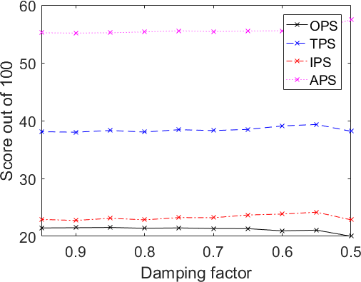
(b) AMP/Perceptual

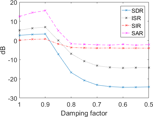
(c) VAMP/Non-perceptual

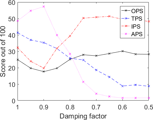
(d) VAMP/Perceptual

Fig. 1: Performance of undamped AMP and VAMP as the damping factor varies. Scores are averaged for mixtures with four sources. Damping does not appear to affect AMP, but it has a significant effect on VAMP, as the performance suddenly drops after $\theta\leq 0.9$.

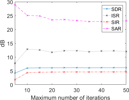
(a) AMP/Non-perceptual

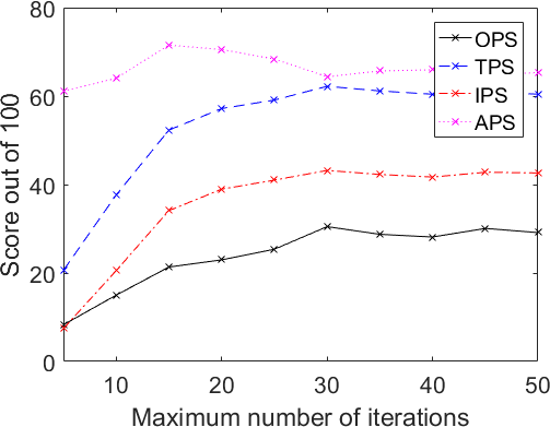
(b) AMP/Perceptual

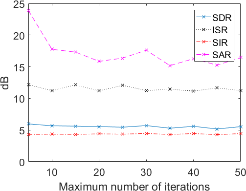
(c) VAMP/Non-perceptual

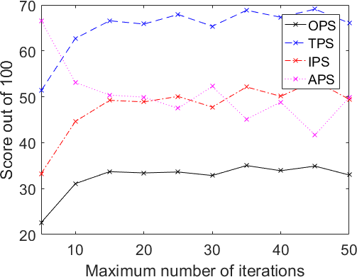
(d) VAMP/Perceptual

Fig. 2: Performance of undamped AMP and VAMP as the maximum number of iterations varies. Scores are averaged for mixtures with three sources. The performance levels or converges after a certain number of iterations, with VAMP converging faster than AMP.

5 Conclusion

In this paper, approximate message passing algorithms were investigated for underdetermined audio source separation. These algorithms can be considered as approximations to belief propagation, offering a probabilistic framework for inferring the sources. Using a Bernoulli-Gaussian prior for the sources in the STFT (time-frequency) domain, we used AMP to solve the sparse linear inverse problem. Since AMP is only accurate for large systems, a block-based approach was taken instead of solving the problem for each sample individually.

Two algorithms known as AMP and VAMP were evaluated with the SiSec dataset and the PEASS toolkit. The results showed that separation is indeed possible using this approach, with AMP performing better than VAMP. In terms of artefact suppression, AMP produced very promising results. This is a desirable property in applications such as hearing assistance, where it is less tolerable for such artefacts to be present. In the future, we would like to apply AMP to convolutive mixtures, for which the block-based approach easily lends itself. Another possible development is structured sparsity, e.g. grouping the real and imaginary coefficients.

References

- [1] P. Bofill and M. Zibulevsky, “Underdetermined blind source separation using sparse representations,” Signal Process., vol. 81, no. 11, pp. 2353–2362, Nov. 2001.
- [2] A. Jourjine, S. Rickard, and O. Yilmaz, “Blind separation of disjoint orthogonal signals: demixing N sources from 2 mixtures,” in Proc. IEEE Int. Conf. Acoust., Speech, Signal Process. (ICASSP), 2000, vol. 5, pp. 2985–2988.
- [3] O. Yilmaz and S. Rickard, “Blind separation of speech mixtures via time-frequency masking,” IEEE Trans. on Signal Process., vol. 52, no. 7, pp. 1830–1847, July 2004.
- [4] D. L. Donoho, A. Maleki, and A. Montanari, “Message-passing algorithms for compressed sensing,” Proc. Nat. Acad. Sci. (PNAS), vol. 106, no. 45, pp. 18914–18919, Nov. 2009.
- [5] M. Bayati, M. Lelarge, and A. Montanari, “Universality in polytope phase transitions and message passing algorithms,” Ann. Appl. Probab., vol. 25, no. 2, pp. 753–822, Feb. 2015.
- [6] D. L. Donoho, A. Maleki, and A. Montanari, “Message passing algorithms for compressed sensing: I. motivation and construction,” in Proc. IEEE Inform. Theory Workshop (ITW), 2010, pp. 1–5.
- [7] S. Rangan, “Generalized approximate message passing for estimation with random linear mixing,” in Proc. IEEE Int. Symp. Inform. Theory (ISIT), 2011, pp. 2168–2172.
- [8] A. Manoel, F. Krzakala, E. W. Tramel, and L. Zdeborová, “Swept approximate message passing for sparse estimation,” in Proc. 32nd Int. Conf. Mach. Learn. (ICML), 2015, pp. 1123–1132.
- [9] S. Rangan, P. Schniter, and A. Fletcher, “On the convergence of approximate message passing with arbitrary matrices,” in Proc. IEEE Int. Symp. Inform. Theory (ISIT), 2014, pp. 236–240.
- [10] J. Vila, P. Schniter, S. Rangan, F. Krzakala, and L. Zdeborová, “Adaptive damping and mean removal for the generalized approximate message passing algorithm,” in Proc. IEEE Int. Conf. Acoust., Speech, Signal Process. (ICASSP), 2015, pp. 2021–2025.
- [11] B. Cakmak, O. Winther, and B. H. Fleury, “S-AMP: Approximate message passing for general matrix ensembles,” in Proc. IEEE Inform. Theory Workshop (ITW), 2014, pp. 192–196.
- [12] S. Rangan, P. Schniter, and A. K. Fletcher, “Vector approximate message passing,” in Proc. IEEE Int. Symp. Inform. Theory (ISIT), June 2017, pp. 1588–1592.
- [13] T. Xu and W. Wang, “A compressed sensing approach for underdetermined blind audio source separation with sparse representation,” in Proc. IEEE/SP 15th Workshop Statist. Signal Process., 2009, pp. 493–496.
- [14] J. B. Allen, “Short term spectral analysis, synthesis, and modification by discrete Fourier transform,” IEEE Trans. Acoust., Speech, Signal Process., vol. 25, no. 3, pp. 235–238, June 1977.
- [15] F. J. Harris, “On the use of windows for harmonic analysis with the discrete Fourier transform,” in Proc. IEEE, 1978, vol. 66, pp. 51–83.
-
[16]
S. Rangan, A. Fletcher, V. Goyal, et al.,
“GAMPmatlab,”
https://sourceforge.net/projects/gampmatlab/. - [17] J. Vila and P. Schniter, “Expectation-maximization Bernoulli-Gaussian approximate message passing,” in Proc. 45th Asilomar Conf. Signals, Syst., Comput. (ASILOMAR), 2011, pp. 799–803.
- [18] E. Vincent, S. Araki, and P. Bofill, “The 2008 signal separation evaluation campaign: A community-based approach to large-scale evaluation,” in Proc. 8th Int. Conf. Independent Component Analysis, Signal Separation, 2009, pp. 734–741.
- [19] S. Araki, A. Ozerov, V. Gowreesunker, et al., “The 2010 signal separation evaluation campaign (SiSEC2010): Audio source separation,” in Proc. 9th Int. Conf. Latent Variable Analysis, Signal Separation, 2010, pp. 114–122.
- [20] V. Emiya, E. Vincent, N. Harlander, and V. Hohmann, “Subjective and objective quality assessment of audio source separation,” IEEE Trans. Audio, Speech, Language Process., vol. 19, no. 7, pp. 2046–2057, Sept. 2011.
- [21] E. Vincent, R. Gribonval, and C. Fevotte, “Performance measurement in blind audio source separation,” IEEE Trans. Audio, Speech, Language Process., vol. 14, no. 4, pp. 1462–1469, July 2006.