Polarimetry and Spectroscopy of the ‘Oxygen Flaring’ DQ Herculis-like nova: V5668 Sagittarii (2015)

Abstract

Context. Classical novae are eruptions on the surface of a white dwarf in a binary system. The material ejected from the white dwarf surface generally forms an axisymmetric shell of gas and dust around the system. The three-dimensional structure of these shells is difficult to untangle when viewed on the plane of the sky. In this work a geometrical model is developed to explain new observations of the 2015 nova V5668 Sagittarii.

Aims. We aim to better understand the early evolution of classical nova shells in the context of the relationship between polarisation, photometry and spectroscopy in the optical regime. To understand the ionisation structure in terms of the nova shell morphology and estimate the emission distribution directly following the light-curve’s dust-dip.

Methods. High-cadence optical polarimetry and spectroscopy observations of a nova are presented. The ejecta is modelled in terms of morpho-kinematics and photoionisation structure.

Results. Initially observational results are presented, including broadband polarimetry and spectroscopy of V5668 Sgr nova during eruption. Variability over these observations provides clues towards the evolving structure of the nova shell. The position angle of the shell is derived from polarimetry, which is attributed to scattering from small dust grains. Shocks in the nova outflow are suggested in the photometry and the effect of these on the nova shell are illustrated with various physical diagnostics. Changes in density and temperature as the super soft source phase of the nova began are discussed. Gas densities are found to be of the order of 10⁹ cm^-3 for the nova in its auroral phase. The blackbody temperature of the central stellar system is estimated to be around $2.2\times 10^{5}$ K at times coincident with the super soft source turn-on. It was found that the blend around 4640 $\rm{\AA}$ commonly called ‘nitrogen flaring’ is more naturally explained as flaring of the O ii multiplet (V1) from 4638 - 4696 $\rm{\AA}$, i.e. ‘oxygen flaring’.

Conclusions. V5668 Sgr (2015) was a remarkable nova of the DQ Her class. Changes in absolute polarimetric and spectroscopic multi-epoch observations lead to interpretations of physical characteristics of the nova’s evolving outflow. The high densities that were found early-on combined with knowledge of the system’s behaviour at other wavelengths and polarimetric measurements strongly suggest that the visual ‘cusps’ are due to radiative shocks between fast and slow ejecta that destroy and create dust seed nuclei cyclically.

1 Introduction

Classical novae are a sub-type of cataclysmic variable and are characterised by light-curves and spectra whose development are followed from radio through to gamma wavelengths. Strope et al. (2010) classified a variety of optical light curves and provided physical explanations for many of their features and more recently Darnley et al. (2012) laid out a new classification scheme for novae based on the characteristics of the companion star.

Novae are known to be a distinct stellar event and in their simplest terms are considered as either fast (t₃ $\textless$ 20 days) or slow (t₃ $\textgreater$ 20 days, where t₃ is the time taken for a nova’s magnitude to decrease by 3). Fast novae occur on more massive white dwarfs than slow novae and require less accreted matter in order to ignite the thermonuclear runaway and experience higher ejection velocities, e.g. Yaron et al. (2005). Slower novae counterparts typically occur on lower mass white dwarfs, eject more previously-accreted-material during eruption and the outflow has lower ejection velocities which creates rich dust formation factories, e.g. Evans et al. (2014). These objects are well observed during eruption where optical photometry and spectroscopy are the most thoroughly practiced approaches. Although in recent times X-ray observations have become more common with the advent of $\it{Swift}$, see Schwarz et al. (2011).

Novae have long been observed in terms of spectroscopy dating back to the 1891 nova T Aur (Vogel, 1893), and have been systematically studied since Williams et al. (1994). A user guide on spectroscopy of classical novae is also available (Shore, 2012). A commonly adopted classification scheme for nova spectroscopy is known as the Tololo scheme, first presented by Williams et al. (1991). Nova spectra are characterised by several observable stages during their eruption and the progression through these spectral stages (i.e. skipping some or showing critical features in others) gives the nova its spectral fingerprint. The spectral stages in the Tololo scheme are defined by the strength of the strongest non-Balmer line, as long as the nova is not in its coronal stage (given the designation C, defined as when [Fe x] 6375 $\rm{\AA}$ is stronger than [Fe vii] 6087 $\rm{\AA}$), whether they are permitted lines, auroral or nebular (P, A or N respectively). Depending on which species is responsible for the strongest non-Balmer transition in the optical spectrum, the formulation (h, he, he⁺, o, ne, s…) is denoted by a subscript. At any time, if the O i 8446 $\rm{\AA}$ line is present then an ‘o’ is included as a superscript in the notation. Developing spectral stages of novae are also often described as the pre-maximum spectrum, principal, diffuse enhanced, orion, auroral and nebular (in order of appearance) see e.g. Warner (1995); Anupama (2012). Changes in the appearance of nova spectra are due to temperature, expansion, clumping, optical depth effects, contribution from the companion star and orbital phase.

To date, polarimetric observations of novae have shown intrinsically low levels of absolute polarisation and are therefore difficult to quantify and understand. Polarimetric observations of novae began over fifty years ago during early development of the technique as it applies to astronomical objects. V446 Her was the first nova to be observed and a constant linear polarisation was measured to within 0.13$\%$ in absolute polarisation degree (Grigorian & Vardanian, 1961).

Observations of novae tend to demonstrate low polarisation arising from several astrophysical processes such as clumpiness, scattering by small dust grains, electron scattering and polarisation in resonance lines, or a combination of these processes.

The dust formation episode in novae is identified as a deep dip in the visual light curve, corresponding to a rise in the thermal infrared, known commonly as the ‘dust-dip’. As the newly-formed optically-thick dust shell expands away from the central system the visual brightness increases once again, and although the recovery is often smooth it is possible to have cusp-shaped features in this part of the light-curve that are often associated with radiative shocks in the ejecta (Lynch et al., 2008; Kato et al., 2009). These shocks are expected in part to contribute to the ionisation of the nova ejecta as well as the shaping, clumping, dust formation and destruction processes. Shocks are detectable in the radio, gamma and X-ray wavelength regimes (Metzger et al., 2014). The role that shocks have in the early evolving nova outflow has been analysed in detail by Derdzinski et al. (2017), who found that consequences of a shock treatment over a purely homologous photoionised expansion lead to higher densities and lower temperatures in certain parts of the ejecta.

DQ Her is an historically important nova-producing system. Following a major observed eruption in 1934, DQ Her became the archetype for rich dust-forming slow novae. It was one of the first nova to be followed with high-cadence spectroscopic observations Stratton & Manning (1939), and this data was later used to classify nova spectra into 10/11 subclasses by McLaughlin (1942). Walker (1954) showed a binary and since then it has been established that all classical nova-producing systems contain binary cores. Kemp et al. (1974) found variation in linear polarisation of the quiescent DQ Her system and Swedlund et al. (1974) presented variations in the circular polarisation of DQ Her. Both the circular and linear polarisation variation were found to correspond to twice the white dwarf period of 71 s. In a later paper, Penning et al. (1986) found no variation in the circular polarisation of DQ Her that corresponded to the white dwarf’s orbital-spin period, although no reference was made to the work of either Kemp et al. (1974) or Swedlund et al. (1974).

The subject of the paper is V5668 Sgr (PNV J18365700-2855420 or Nova Sgr 2015b) a slow-evolving dust-forming nova and is a clear example of a DQ Her-like nova. V5668 Sgr was confirmed as an Fe ii nova in spectra reported by Williams et al. (2015) and Banerjee et al. (2015) after it was discovered at 6.0 mag on 2015 March 15.634 (Seach, 2015). As a close and bright nova with a deep dust-dip, this object might be expected to produce a visible shell discernible from the ground within ten years using medium class telescopes. Banerjee et al. (2016) calculated a distance of around 1.54 kpc to the nova system. The distance was calculated by fitting an 850 K blackbody to their dust SED on day 107.3 post-discovery to find $\rm{\theta_{bb}}$ and assuming an expansion velocity of 530 km s^-1, where $\rm{\theta_{bb}}$ is the blackbody angular diameter. It was also found in the same work that V5668 Sgr was a rich CO producer as well as one of the brightest novae (apparent magnitude) of recent times, reaching 4.1 mag at visual maximum. As V5668 Sgr is a clear example of a DQ Her-like nova light curve (see Fig. 1), it is interesting to look for similarities between the two systems. A 71 $\pm$ 2s oscillation in the X-ray flux was observed by Page et al. (2015) and this value may be related to the white dwarf spin period in the V5668 Sgr system, which is coincidental to the value of 71 s for the white dwarf spin period of DQ Her, e.g. Swedlund et al. (1974). This nova type are generally associated with eruptions on the surface of CO white dwarfs and their maxima can be difficult to identify due to their jitter or oscillation features superimposed on an otherwise flat-top seen immediately prior to a distinguishable dust formation episode. Throughout this work, we refer to this early phase as the ‘flat-top-jitter’ phase. The flat-top-jitter phase of the V5668 Sgr eruption was monitored by Jack et al. (2017), where it was seen that the appearance of an increasing number of ‘nested P-Cygni profiles’ in individual spectral lines could be associated with multiple ejection episodes or evolving components.

Several constraints of the system during the deepest part of the dust-dip are presented by Banerjee et al. (2016) from infrared high-cadence observations. Their observations resulted in a gas/dust temperature of $\approx$ 4000 K, a dust mass of $1\times 10^{-8}$ M_⊙, and an expansion velocity of 530 km s^-1. Banerjee et al. (2016) found a black body diameter of the dust shell to be 42 mas on day 107.3. This estimate is sensitive to the fitted black body temperature of 850 K to the dust SED presented in Fig. 4 (right panel) of their work and corresponds to a physical diameter of $\approx$ $9.6\times 10^{14}$ cm on the sky.

Data is presented here from five nights of polarimetric observations acquired during the nova’s permitted spectral phase with the Dipol-2 instrument mounted on the William Hershel telescope (WHT) and the La Palma KVA stellar telescope. The observations were obtained directly following the deep dust minimum and the nova’s rise through its observed cusps. The nova shell of V5668 Sgr is not yet resolvable with medium-sized ground-based telescopes given the recent eruption, however we present a pseudo 3D photoionisation model based on 1D cloudy (Ferland et al., 2013) models to demonstrate the ionisation structure of V5668 Sgr following its dust formation episode. Throughout the course of this work observations are mentioned in terms of days since discovery of the nova source and all quoted wavelengths are Ritz air wavelengths from the NIST database (Shen et al., 2017).

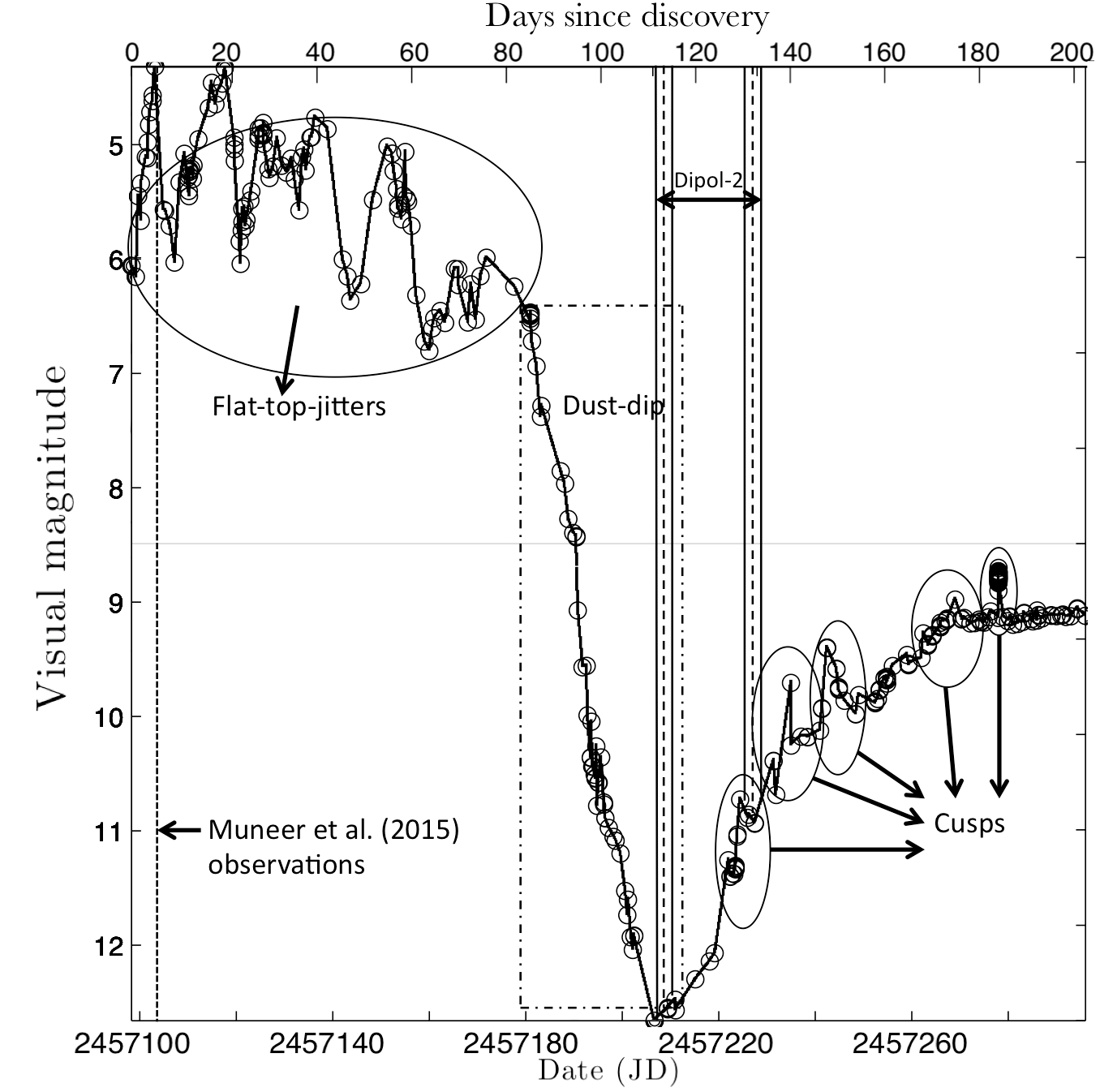
Figure 1: V5668 Sgr AAVSO light curve. Marked are the three major light-curve stages observable in the figure, i.e. the flat-top-jitters, the deep dust-dip and the cusp shaped features seen on the rise out of the dust-dip. Marked are the times of polarimetric observations of the nova by both the Muneer et al. (2015) team and those presented in this paper, i.e. the Dipol-2 measurements. The y-axis demonstrates the change in visual magnitude whereas the x-axis contains the Julian date on the bottom and days since discovery on the top.

2 Observations

2.1 Polarimetry

The polarisation measurements of V5668 Sgr after the dust-dip stage were made with the Dipol-2 polarimeter mounted on the 4.2m WHT telescope during three nights: MJD2457207, 2457208 and 2457210 (days 111, 112 and 114 post-discovery). Two more measurements were recorded two weeks later with the 0.6m KVA stellar telescope (on MJD2457226 and 2457229, i.e. days 130 and 133 post-discovery, see Fig. 2). Each night, 16 measurements were made of Stokes parameters q and u and the weighted mean values computed. The exposure time was 10 sec for the WHT and 30 sec for the KVA. The polarisation data, which have been acquired simultaneously in the standard B, V and R pass-bands, are given in Table 1.

Description of the polarimeter design is given by (Piirola et al., 2014). Detailed descriptions of the observational routine and data reduction procedure can be found in Kosenkov et al. (2017).

For determination of instrumental polarisation, we have observed a set of nearby ( d $<$ 30 pc) zero-polarised standard stars. The magnitude of instrumental polarisation for Dipol-2 mounted in Cassegrain focus on both telescopes was found to be less than 0.01$\%$ in all pass-bands, which is negligible in the present context. For determination of the zero-point of polarisation angle, we have observed highly polarised standards HD 161056 and HD 204827. The internal precision is $\scriptstyle\sim$0.1^∘, but since we rely on published values for the standards, the estimated uncertainty in determination of the zeropoint is less than 1 - 2^∘.

Effects that may be responsible for the observed variations in polarimetric measurements over the course of the observations include uncertainties regarding the standards, lunar proximity or orbital phase. Although, sky background polarisation is directly eliminated. Lunar proximity and seeing effects would add noise and contribute to larger errors rather than systematic deviations.

Table 1: Polarimetry observations gathered during and rising out of the deep-dust dip experienced by this nova with the Dipol-2 instrument.

Date (J.D.)	Telescope	Filter	Pol (%) $\pm$ err	P.A. (deg) $\pm$ err
2457207.5	WHT	B	1.699 $\pm$ 0.017	144.1 $\pm$ 0.3
2457207.5	WHT	V	0.601 $\pm$ 0.014	144.9 $\pm$ 0.7
2457207.5	WHT	R	0.344 $\pm$ 0.007	148.3 $\pm$ 0.6
2457208.5	WHT	B	1.471 $\pm$ 0.015	145.4 $\pm$0.3
2457208.5	WHT	V	0.566 $\pm$ 0.012	148.3 $\pm$ 0.6
2457208.5	WHT	R	0.330 $\pm$ 0.006	153.2 $\pm$ 0.5
2457210.6	WHT	B	1.338 $\pm$ 0.018	147.6 $\pm$ 0.4
2457210.6	WHT	V	0.565 $\pm$ 0.023	151.3 $\pm$ 1.2
2457210.6	WHT	R	0.357 $\pm$ 0.009	152.4 $\pm$ 0.7
2457226.5	KVA	B	0.723 $\pm$ 0.088	152.0 $\pm$ 3.5
2457226.5	KVA	V	0.616 $\pm$ 0.097	155.0 $\pm$ 4.5
2457226.5	KVA	R	0.416 $\pm$ 0.051	151.7 $\pm$ 3.5
2457229.5	KVA	B	1.132 $\pm$ 0.106	170.9 $\pm$ 2.7
2457229.5	KVA	V	0.770 $\pm$ 0.092	183.1 $\pm$ 3.4
2457229.5	KVA	R	0.440 $\pm$ 0.035	177.3 $\pm$ 2.2

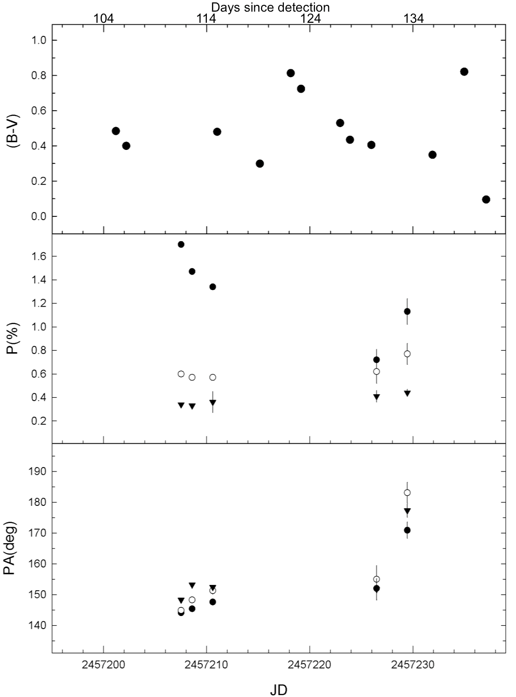
Figure 2: Panels from top to bottom: (B-V) colour index as derived from AAVSO data during Dipol-2 observation epoch; the middle panel shows the measured absolute polarisation degree in percentage and the bottom panel shows the recorded position angles for the polarisation measurements. The filled circles shows the data for the B-band, hollow circles - V-band and filled triangles - R-band. Days since outburst are marked along the top x-axis. The error bars ($\pm$1$\sigma$) are smaller than the plotting symbol for the WHT data (days 111-114 post outburst).

2.2 Photometry

Polarimetric observations were collected on 22 nights with the RINGO3 polarimeter (Steele et al., 2006) on the LT (Steele et al., 2004) spanning days 113-186 after eruption detection. Unfortunately, it was found that the instrument’s performance at low levels of absolute polarisation were not sufficient in the present context due to intrinsic non-negligible changes in the value of the EMGAIN parameter of the EMCCD detectors at the eight different positions of the polaroid rotor. This being said, the observations were of sufficient quality to perform differential photometry. The RINGO3 passbands were designed to incorporate the total average flux of a gamma-ray burst equally across the three bands and are thus unique to the instrument. The bands: known as red, green and blue, correspond to wavelength ranges 770-1000 nm, 650-760 nm and 350-640 nm respectively - roughly equivalent to the Johnson-Cousins I, R and B+V optical filter bands (Steele et al., 2006).

The integrated flux from the 8 rotated exposures (S1) from each night of observation of the nova was recorded. The four brightest field stars were chosen for photometric comparison. The same field stars were not always within the frame on different dates. In essence, differential photometry was conducted with each one of the four field stars and the derived values were found to agree closely, in the end the brightest of the field stars was chosen as it gave the most reliable results and was present in the most frames across the different filters on the relevant nights. The results of this analysis can be seen in Fig. 3. Performing photometry on this dataset allows for information to be gained on the nova systems behaviour during the sparsely populated AAVSO data during the Dipol-2 polarimetric as well as the densest auroral stage, during the FRODOSpec spectroscopic observation epochs.

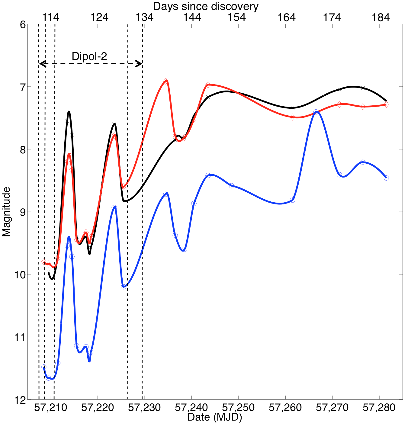
Figure 3: Results of differential photometry from the RINGO3 polarimetric data. The cusps on the rise out of the nova’s dust-dip are clearly visible in the plot. The first cusp corresponds to the grain destruction seen in the Dipol-2 data days 111 - 114 post-discovery. The rise on the third cusp feature visible in the plot is from the grain growth period suggested by the Dipol-2 observations, these observations lie between the dashed lines on the plot. The lines are colour-matched with the RINGO3 bands, blue is blue, red is red and green is black.

2.3 Spectroscopy

Using FRODOSpec (Barnsley et al., 2012) mounted on the Liverpool Telescope (Steele et al., 2004) in low resolution mode, spectra were taken over 103 nights from outburst detection until day 822 post outburst. Data acquired with FRODOSpec are reduced and wavelength calibrated through the appropriate pipeline, detailed by Barnsley et al. (2012). The spectra were flux calibrated using standard routines in iraf (Tody, 1993) against a spectrum of G191-B2B taken on 30 Sept 2015 using the same instrument setup. The standard spectral data was obtained from Oke (1990). All spectra were taken in the low-resolution mode of FRODOSpec except for two dates, these being day 411 and 822 post-discovery, whose observations were collected in high-resolution mode. The resolving power of the low-resolution mode are 2600 for the blue arm and 2200 for the red arm. The low-resolution mode in the blue arm therefore gives a resolution of around 1.8 $\rm{\AA}$ or 120 km s^-1. High resolution mode has a resolving power of 5500 in the blue arm in 5300 for the red arm. The spectroscopic data were analysed using SPLOT and other standard routines in iraf. As the vast majority of the spectra involved are from the low resolution mode a systematic error of up to 20% is expected as well as a 10% random error.

3 Analysis and Results

3.1 Polarimetry

The wavelength dependence of polarisation (sharp increase towards the blue) gives strong support for Rayleigh scattering as the primary source for the observed polarisation after the dust formation stage; see Walter (2015); Gehrz et al. (2015) for more on this particular nova’s primary dust formation episode. The directions of polarisation in the B, V and R bands are close to each other for the five dates, which suggests an intrinsic nature to the observed polarisation. The interstellar component is small even in the V and R bands because the angle of polarisation in the V and R bands are always close to that in the B-band.

Unfortunately, photometry data at the dates when the polarisation with the Dipol-2 instrument was measured is not available. As can be seen from Fig. 2, however, the color index (B-V) did not change significantly over the range of dates from when the absolute polarisation was measured. Consequently, the rapid changes in the B-band polarisation seen on days 111-114 and 130-133 post-discovery are not due to decrease or increase of the fraction of the polarised scattered light in the system.

Variations in the absolute polarimetry over the five nights observing of V5668 Sgr with Dipol-2 covered days 111-133 post-discovery are after the formation of dust and during the local minimum in the transitional-stage of the optical light curve. The observed flux in the R-band is likely dominated by H$\alpha$ in these observations. The most probable explanation for the observed variations in the absolute polarisation is the small dust particles which are responsible for the appearance of the polarised scattered light. During days 111-114 post-discovery, the destruction phase could be observed while during 130-133 post-discovery, the creation phase was recorded.

X-ray counts increased during the observations reported here, see Page et al. (2015), Gerhrz et al. (in prep.), exposing the nova shell to a harsher radiation field. Infrared SOFIA observations (Gehrz et al., 2015), that coincided with the commencement of the observations presented here, revealed that the dust emission on day 114 post-discovery had increased since day 83 post discovery and that a reduction in grain temperature suggested rapid grain growth to sub-micron radii. These observations suggest that the hydrogen emission in the NIR was blanketed by the dust and the effect of this can be seen in the strengthening of the Paschen series, see Figs. 5 & 6. Emission at this time is expected to arise from a cold dense shell as well as hotter, less-dense ejecta, see Derdzinski et al. (2017). Gehrz et al. (in prep) are presenting $\it{Swift}$ and SOFIA observations of this nova covering the IR, UV and X-ray behaviour of the nova system.

UBVRI polarimetry before the dust-dip, taken during the flat-top-jitter phase over the first observed major primary jitter, was reported by Muneer et al. (2015), providing knowledge of the absolute polarisation of the system before the major dust formation event. Although the measurements by Muneer et al. (2015) are not corrected for interstellar polarisation toward the source, the correction is not made here either. The earlier Muneer et al. (2015) results are lower than those of the Dipol-2 observations directly following the dust-dip, with position angle (P.A.) measurements being consistent. The earlier observations with lower recorded absolute polarisation of Muneer et al. (2015) fit with electron scattering or interstellar polarisation, as expected before the dust formation episode. Of interest regarding the observations of Muneer et al. (2015) is that between days 2 - 4 post-discovery, P.A. of the polarisation varies between roughly 150^o and 10^o (i.e. 190^o) - very similar to that in the Dipol-2 measurements, see Table 1. In the observation presented here, values between 144^o - 183^o were found for the P.A. The origin location of the source of the polarisation is indicative of the opening angle of the component, be it the equatorial or polar nova shell components is unknown. The work of Derdzinski et al. (2017) would suggest the opening angle to be related to the equatorial disk.

These observations can be understood in terms of dust resulting from seed nuclei that formed during the optical dust-dip and increase of the density in the forward shock zone. Lynch et al. (2008); Kato et al. (2009) and Strope et al. (2010) discuss cusps as possibly arising from shocks in the nova outflow. Since V5668 Sgr is a slow nova, strong shaping of the ejected nova material is expected. A strong correlation in position angle of the polarisation is needed throughout the observed epochs if it is related to either the equatorial or polar components of the nova outflow. The shock passes through the layer of fresh-formed small dust grains and destroys them, yet retaining seed nuclei, thus allowing for the process to repeat over the next shock cycle. $\it{Swift}$ X-ray data (Gehrz et al. 2017, in prep) shows the X-ray count rising on entering the dust-dip and increasing again when the cusps start (post dust-dip-minimum). The phenomenology of the hard X-rays can be understood in the context of shocks and sweeping up material, allowing the local densities to increase, which creates favourable conditions for dust formation. The soft component of the X-ray emission should be due to continued nuclear burning on the surface of the central white dwarf (Landi et al., 2008), whereas the hard component is expected to arise from shocks, e.g. Metzger et al. (2014).

Gamma-ray emission was observed for the V5668 Sgr nova event and is described by Cheung et al. (2016). The emission of gamma-ray photons of energy $\geqslant$100 MeV lasted around 55 days, longer and intrinsically fainter than any of the six other nova observed to produce gamma-ray emission. The onset of gamma-rays occurred two days following the first optical peak and were followed for 212 days. Due to low photon counts the team who discovered the sixth confirmed gamma-ray nova, were unable to correlate gamma variability with that in the optical, although the gamma emission peaks during the third major jitter (around days 30 - 40 post-discovery) on the nova’s otherwise flat-top light curve. The Fermi-LAT observations of this nova ended one month previous to the observations discussed here and before V5668 Sgr’s dust formation event.

3.2 Spectroscopy

Observed spectra were calibrated and subsequently interpreted using published results from the literature and cloudy simulations (Ferland et al., 2013). Shocks suggested by the polarimetry and multi-wavelength observations discussed in 3.1.

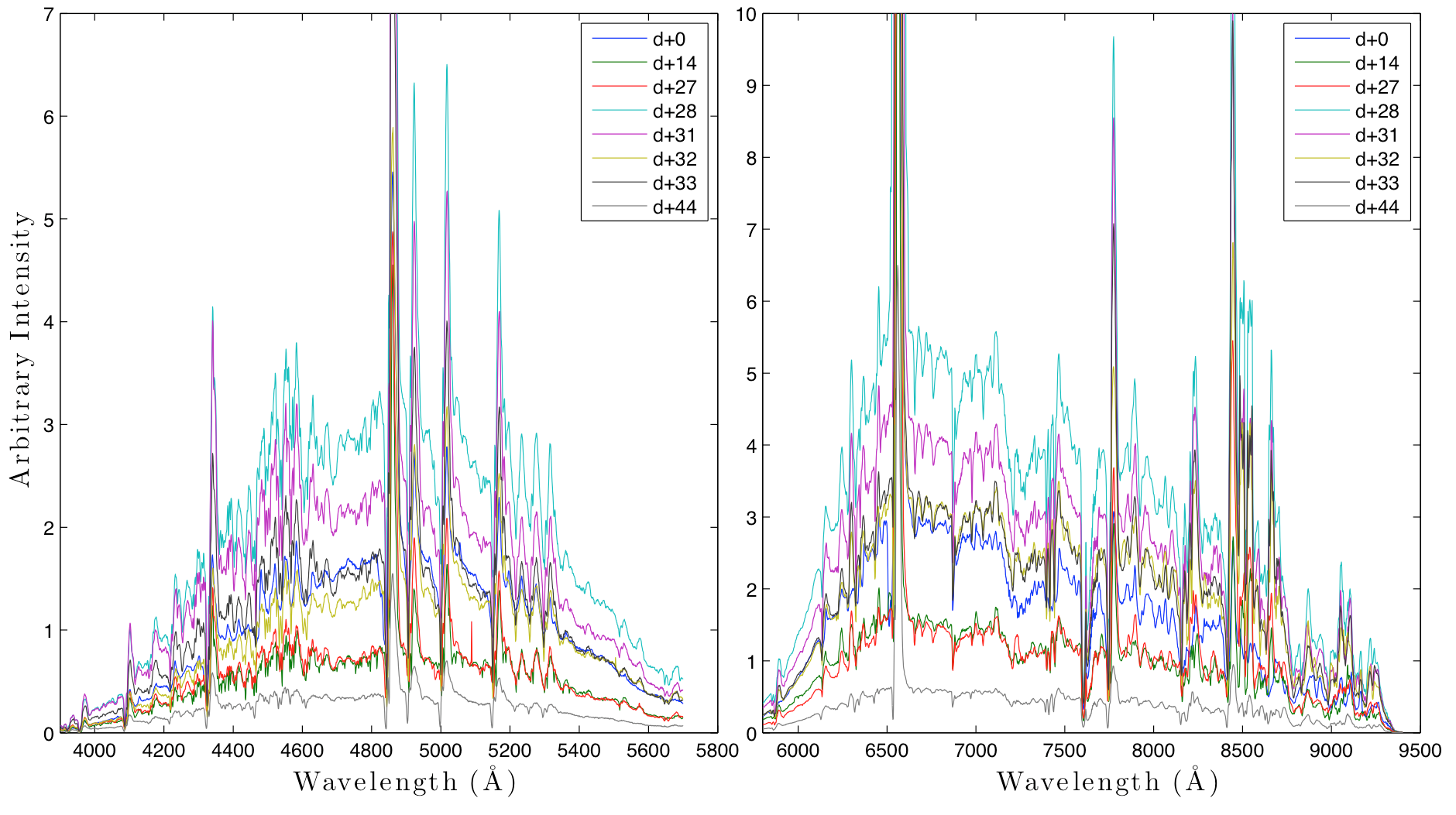
Figure 12: Spectroscopy from the flat-top-jitter phase in the FRODOSpec blue and red arms. Dates post-discovery are marked on the upper right hand ride of the plot

The earliest spectra observed here are interesting from the point of view of a suggestion of multiple components during the flat-top-jitter phase. A spectrum obtained on day 0 post-discovery shows P-cygni profiles with absorption components at -1200 km s^-1. Further observations 14 days later revealed two absorption components in the strongest spectral lines with each having a measured velocity of -950 and -520 km s^-1 in the Balmer lines. In spectra taken in mid April, the highest velocity component of the maximum spectrum increased again to approximately -1125 km s^-1 and with a new lower-velocity component of -610 km s^-1. These observations hint at optical depth effects where in the 14 days post-discovery spectrum, the inner side of the expanding shell is visible. Then by day 27, an outer shell section may becomes visible when three absorption components appear with velocities of -554, -945 and -1239 km s^-1, respectively. The expanding shell is still expected to be radiation bound at this stage due to the high densities present. On day 28, the observed velocities decrease to -507, -887 and -1065 km s^-1. The next spectrum was observed on day 31 with FRODOSpec, where it can be seen that the middle absorption component disappeared and leaving two components at -537 and -1047 km s^-1. In spectra taken on days 32 and 33 post-discovery, a slight increase is seen in the absorption components which then levels off until the absorption systems disappear and are replaced by emission wings. In the subsequent spectra it appears that only the slower component remains visible as part of the expanding shell. It is worthy to note that the appearance of additional absorption components appear to be correlated with the local maxima in the nova’s early light curve. The evolution of the aforementioned absorption components can be seen in Figs. 12 & 13. The Ca ii lines during these early days display a similar structure to Balmer and nebular [O iii] lines at late times.

The spectra presented in Figs. 5 and 6 show 10 nights: from 6 July to 14 August. It was found that the earlier July spectra (days 114, 116, 120, 122 and 123 post-discovery), see Fig. 5, are all quite similar in appearance and it can be noted how the observed flux from the system recovers. These five spectra correspond to the early-rise out of the dust-dip while the shell is known to be mostly optically thick, exhibited by the presence of strong permitted lines.

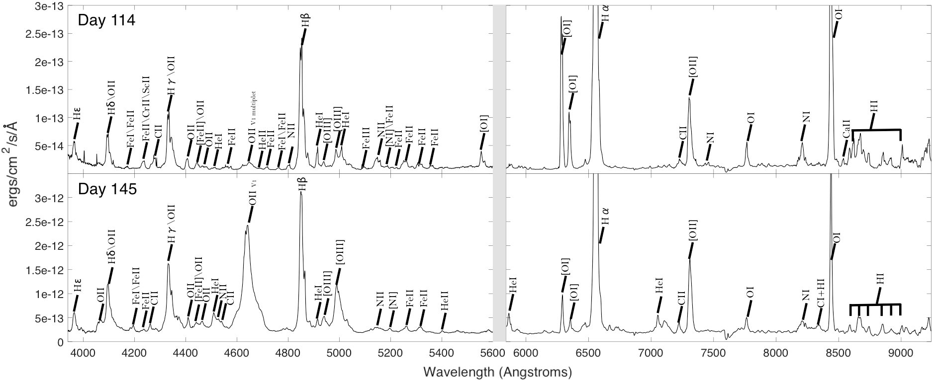
Figure 4: Spectra showing the two main spectroscopic stages observed during the polarimetric observations. Note the fall in O i corresponding to a rise in O ii and O iii lines.

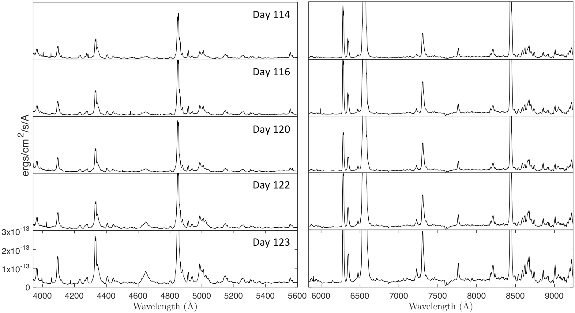
Figure 5: Early July 2015 spectra from FRODOSpec with the blue arm spectra in the left hand series and red arm on the right. Spectra were flux calibrated by Dr. Steve Williams, and are all scaled to the bottom panel of each column. Note the change in flux over the dates.

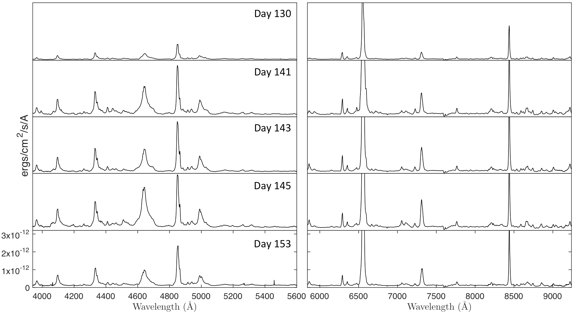
Figure 6: Same as in Fig. 5 except for spectra taken in late July and early August 2015, using FRODOSpec. Note the flaring feature in the blue arm of the spectra identified in this work as arising from the O ii V1 multiplet, see Section 3.4.

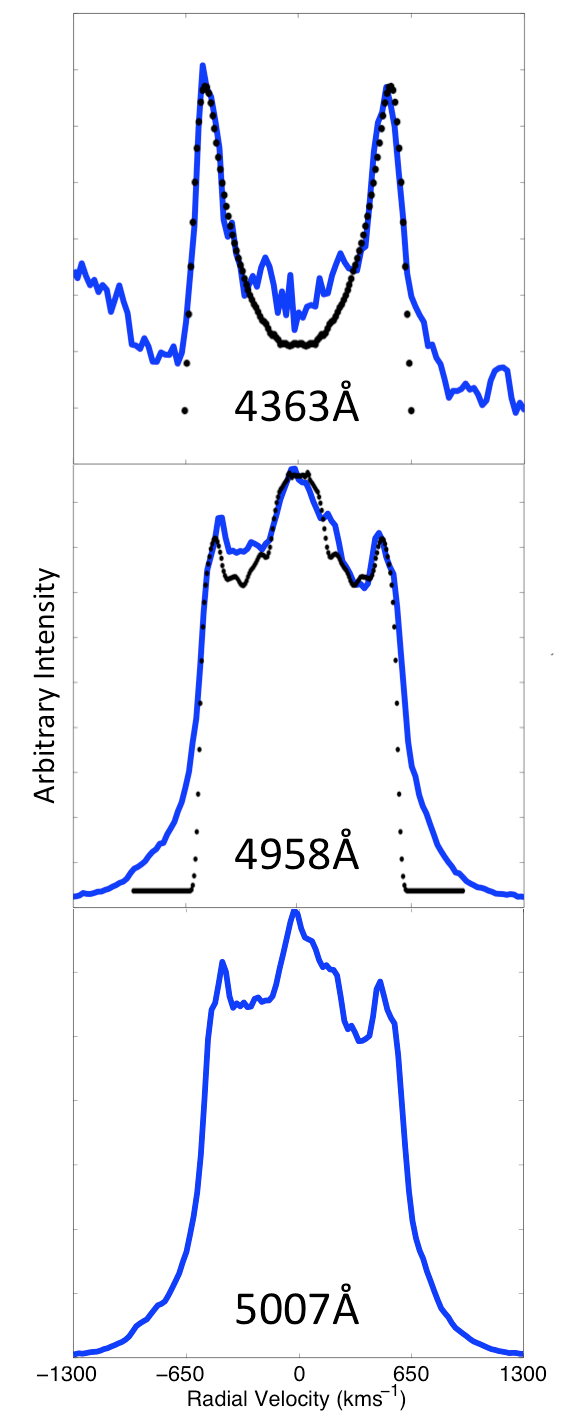
Figure 7: Spectra of [O iii] nebular and auroral lines on day 822 post-discovery. The observed line profiles (blue-solid lines) were used in the fitting of a morpho-kinematical model with the shape software, seen as the overlaid black dots. The auroral line is fitted with an equatorial disk whereas the nebular lines fit an equatorial waist and polar cones morphology with a Hubble outflow velocity law, see Fig. 8.

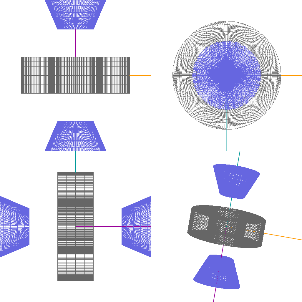
Figure 8: Mesh display of the spatial structure of the nova shell around V5668 Sgr as determined from the nebular [O iii] line shapes with the shape software, see Fig. 7. The four panels show different orientations of the structure, the bottom-right-hand-panel shows the nova shell placed at the P.A. suggested from the polarimetry and as visualised in the pycloudy renderings seen in Fig. 11. If the detected polarisation has its origin in the equatorial waist then the shell should be titled at 90^o in the plane of the sky. The saddle shaped 4363 $\rm{\AA}$ [O iii] line feature, as well as other higher excitation species, can be understood as arising from the equatorial-ring-waist.

During the optical light curve’s ascension out of the dust-dip, the most interesting changes are observed in the spectra from 130, 141, 143, 145 and 153 post discovery (see Fig. 6). The final three spectra presented from days 143, 145 and 153 following the eruption straddle a major cusp on the way out of the nova’s visual dust-dip, see Fig. 3. As discussed in Section 3.1, these cusps are commonly associated with shocks that occur in the immediate aftermath of the eruption. The most striking feature has been referred to as ‘nitrogen flaring’ in many previous works, see e.g. Williams et al. (1994); Zemko et al. (2016), around 4650 $\rm{\AA}$.

Over the same time frame, Ca ii is observed to decline whilst He i and He ii are both observed to increase. Fe iii and N i emission strength decrease along with the Paschen series with respect to H$\beta$; for more details see Table 3. The observed behaviour is consistent with the thinning out of ejecta, which subjects the gas mix to harder radiation from the central source.

3.3 Simulations

The spectral development of V5668 Sgr is dominated by the Balmer series plus He, N, O and Fe lines as the nova progresses through its permitted, auroral then nebular spectral stages. According to the Tololo classification scheme the nova is in its P$\rm{{}^{o}_{o}}$ stage during the observations presented in this work. A parameter sweep was conducted using the python wrapper for cloudy (Ferland et al., 2013) known as pycloudy (Morisset, 2013) to examine the line ratios for the hot-dense-thick nova shell that is still close to the burning central system. It was found that the dust shell size of Banerjee et al. (2016), when extrapolated to the expected size for the dates under study in this work, can fit the observed spectra although better fits can be achieved with marginally smaller radii, hinting that the optical emission lines in the optically thick region inner to the dust shell. An implication is that dust clumps should appear and then disappear along the line of sight to the observer, further complicating the analysis.

Initial parameter sweeps were coarse and broad covering densities of $10^{4}-10^{14}$ cm^-3. It was found that densities from $10^{8}-10^{10}$ cm^-3 better explained the structure of the observed spectrum and refined grids were run over these constraints. It is cautioned that, at the densities studied here, the Nussbaumer & Storey (1984) CNO recombination coefficients used are not as reliable since the LS coupling scaling law assumed in Nussbaumer & Storey (1984) diverge for atoms with upwards of two valence electrons.

Fig. 10 shows the results of a parameter sweep including log densities 8.60 - 9.20 in 0.05 dex, and the effective temperature of the central source from $6\times 10^{4}-3.0\times 10^{5}$ K in steps of $2\times 10^{5}$ K. For the parameter sweep pycloudy was used to control cloudy. An average of Fe ii type nova abundances adapted from Warner (1995) were included. The Eddington luminosity of a 0.7 M_⊙ white dwarf was assumed, with r${}_{min}=3.2\times 10^{14}$ cm and r${}_{max}=6.4\times 10^{14}$ cm. As the binary characteristics of this system are not known, a 0.7 M_⊙ white dwarf was chosen based on the turn-on time in X-rays (Gehrz et al. 2017, in prep.) and the nova’s t₂ value in comparison to Fig. 4(c) of Henze et al. (2014). From this type of analysis, it is possible only to say that the white dwarf must be on the lower end of the scale found in nova progenitor systems and that it is most probably a CO white dwarf.

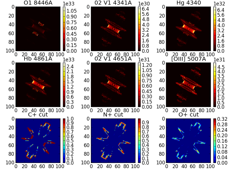
Figure 11: pyCloudy emission model of V5668 Sgr, using nova abundances with the inclination angle set at 85^∘. Conditions for the model were the best derived values from the parameter sweeps assuming luminosity and geometries discussed in Sect. 3.3 for day 141 after discovery. The input shape model is seen in Fig. 8. Volumetric flux units are in ergs s^-1 (colour bars). The x and y axis values are scaled units of physical size, r_min and r_max determined from Banerjee et al. (2016) size on day 107 post-discovery. Clumpiness was simulated using a Perlin noise modifier in shape.

The best fitting densities from the cloudy parameter sweep were in the range $6.3\times 10^{8}$ - $1.0\times 10^{9}$ cm^-3 and an effective temperature of $(1.8-2.4)\times 10^{5}$ K was found for the chosen radial distance, luminosity and abundances for day 141 post discovery. With information from the polarimetry and spectroscopy on conditions present in the expanding nova shell, an attempt to visualise the unresolved shell is presented in Fig. 11, where the models are valid for day 141 post-discovery. In the top six panels of Fig. 11, are the simulated emission of oft-seen oxygen emission lines in erupting nova systems. A comparison of the locality of emission through the shell of the same species is presented in each column of each of these panels. The O i line the strong emission produced from the simulated 6 level oxygen atom line of 8446 $\rm{\AA}$ at the inside of the shell is in good accordance with observations, see also Fig. 9(b). The O ii panels (middle column Fig. 11) simulate both the V1 and V2 multiplets that are shown relative to H$\beta$ in Fig. 9(a) and discussed in 3.4 of this work. The [O iii] panel demonstrate the locality and relative strength of the nebular 5007 $\rm{\AA}$ line. The bottom three panels are, from left to right, ionic cuts of C, N and O, respectively. The shape (Steffen & Lopez, 2006) line profile model fits are to day 822 post-discovery, by when the line structure had frozen, and can be seen in Figs. 7 & 8. A Perlin noise modifier was applied to the hydrogen density distribution of the polar cones and equatorial ring, with the average density being $1.0\times 10^{9}$ cm^-3. The luminosity was set to log(L_⊙) = 4.36, and an effective temperature of $1.8\times 10^{5}$ K was assumed based on the parameter sweep, see Fig. 10. To simulate the nova conditions on day 141 post-discovery an inner radius of $3.2\times 10^{14}$ cm and an outer radius of $6.4\times 10^{14}$ cm were assumed, as in the parameter sweep.

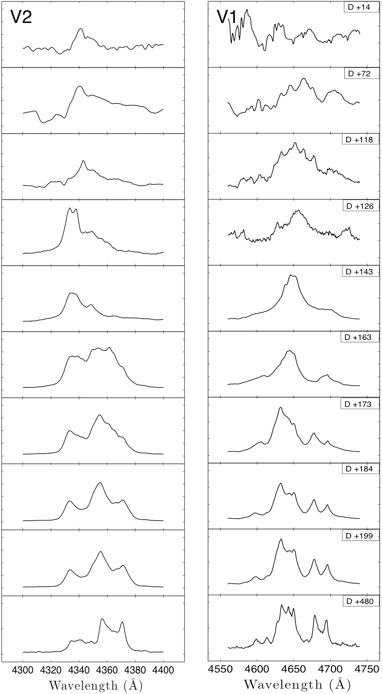
Figure 9: Temporal shape evolution of the blending lines in the area surrounding the 4341 $\rm{\AA}$ and 4650 $\rm{\AA}$ V2 and V1 oxygen multiplets. Days since detection are marked in the top-right-corner of each subplot in the V1 column. The most pronounced flaring episodes are between days 140 - 150 post-discovery. Note in the V1 multiplet column plot (right hand side) a saddle-shaped He ii line at 4686 $\rm{\AA}$ fits the 4676 and 4696 $\rm{\AA}$ lines if they are the red and blue wings of the He ii line.

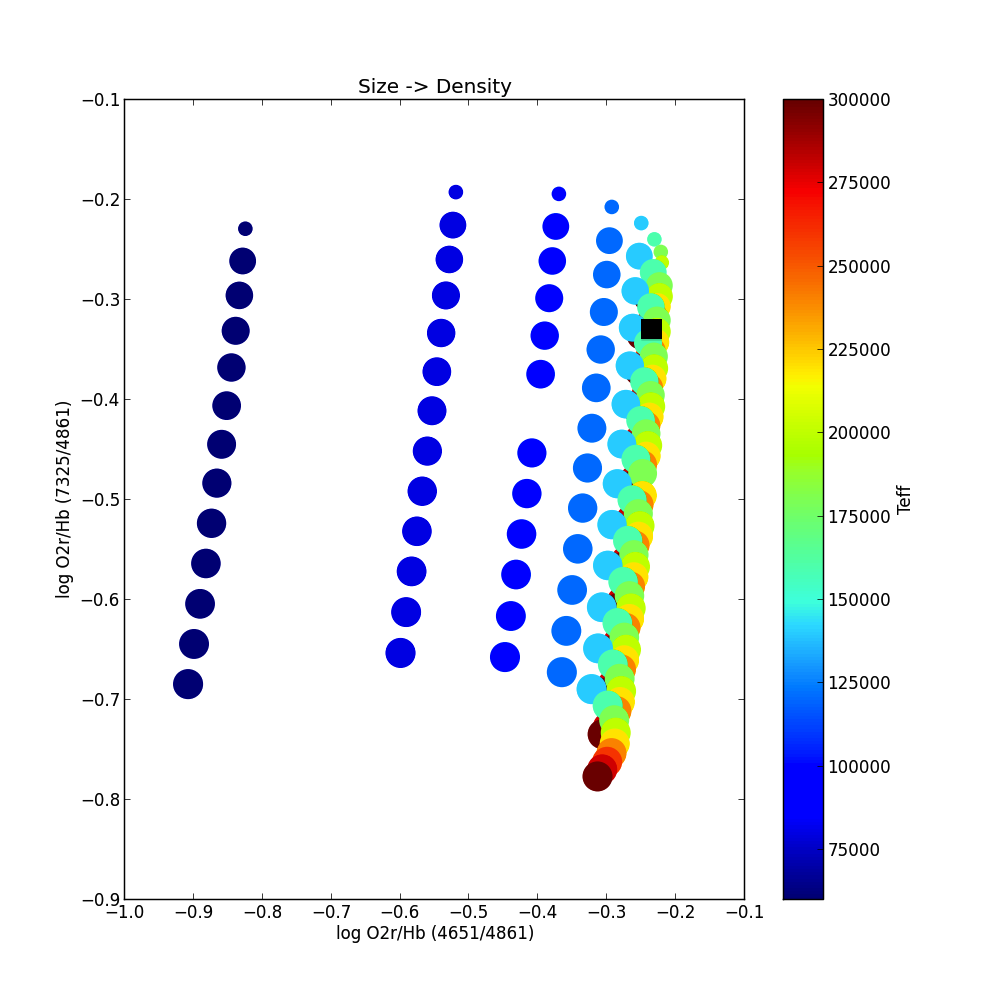
(a)

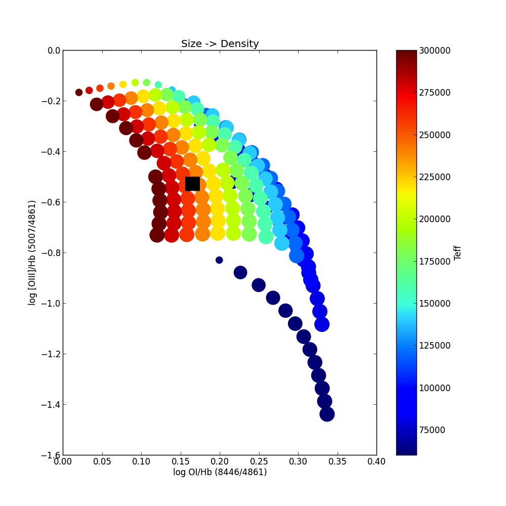
(b)

Figure 10: 1D cloudy parameter sweep of temperature and density of two O ii multiplets relative to H$\beta$. (a) shows O ii 4650 $\rm{\AA}$/H$\beta$ and 7325 $\rm{\AA}$/H$\beta$ diagnostic diagram, whereas (b) shows a [O i] 8446 $\rm{\AA}$/H$\beta$ and [O iii] 5007 $\rm{\AA}$/H$\beta$ diagnostic diagram. Displayed here is a zoomed in version of the parameter sweep covering the log of the nebular densities vary from 8.60 - 9.20 in 0.05 dex, and the effective temperature of the central source from $6\times 10^{4}-3.0\times 10^{5}$ K in steps of $2\times 10^{4}$ K. The black squares mark the measured rations on day 141.

In order to create the shape model, subsequently used for input into pycloudy, three components were used comprising the equatorial waist and the two polar cones, see Fig. 8. The ring-like waist was constructed from a cylinder primitive in which a density, Hubble velocity law and thickness were applied. The two polar features were constructed using cone primitives. The densities applied to the features were estimated using cloudy simulations and the velocity components were found from measuring Doppler broadening of the Balmer emission lines. Emission line structure in fast outflows depend strongly on their velocity field and orientation, shape allows the user to untangle the projection effects. The frozen line shapes of the nebular stage modelled in Fig. 7 are with a inclination of 85^∘ a polar velocity of 940 km s^-1 and equatorial velocity of 650 km s^-1 at their maximum extensions. The proposed structure is similar to that found in other slow novae such as T Aur (see Section ) and DQ Her.

3.4 Oxygen Flaring

It is well known that identification of emission lines in nova eruption spectra is difficult, largely due to blending and large Doppler widths. Table 2 and Fig. 9 demonstrate two cases where important diagnostic lines can easily be confused for other lines or are heavily blended without realisation. Through simple additive arguments based on A_ki values it was found that the O ii V 1 multiplet is comparable to the commonly identified N iii and C iii lines. As there is mention but no modern discussion on O ii in the place of this ‘flaring’ feature, its nature was investigated. Collisional rates are of importance but are not well constrained.

Focusing on the five spectra presented in Fig. 6, we observe the ‘flaring’ episode around 4650 $\rm{\AA}$. This type of flaring episode is often attributed to ‘nitrogen flaring’, although in the photoionisation simulations (Fig. 10) the lines under derived conditions do not favour pumping of N iii lines through the Bowen fluorescence mechanism nor the ionisation and subsequent recombination of the C iii lines. Instead, the recombination of O ii around 4650 $\rm{\AA}$ appears responsible for the majority of the emission, with some contribution expected from pumping of the same and contribution from the Fe iii 4658 $\rm{\AA}$ line. The He ii line at 4686 $\rm{\AA}$ may contribute to the red end of the observed blend, which can be seen in Table 2 and Fig. 4, He ii 4686 $\rm{\AA}$ in a saddle-shaped line profile with emission components around $\pm$ 520 km s^-1 would appear the same as the two longest wavelength lines in the O ii multiplet in the region, i.e. at 4676 and 4696 $\rm{\AA}$. As a consequence of this the presence of He in a nova cannot be confirmed with only the presence of the He ii 4686 $\rm{\AA}$ emission line.

The concept of nitrogen flaring dates back to 1920 when Fowler (1920) identified an ‘abnormal’ strong spectral feature peaking around 4640 - 4650 $\rm{\AA}$. Following this, Mr. Baxandall and W. H. Wright exchanged letters regarding Prof. Fowler’s paper that resulted in an article by Wright entitled “On the Occurrence of the Enhanced lines of Nitrogen in the Spectra of novae” (Wright, 1921). It is noted there that the “4640 stage” occurs first on entering the nebular stage and then can occur recurrently.

In the data presented herein, the flaring episodes reoccur in stages corresponding to the cusps observed in the nova light curve during the transition from the auroral to nebular spectral stages. The proposition that N iii is responsible for this flaring episode is justified in Basu et al. (2010) by a decrease in [O iii] and the “great width of N iii lines corresponding to a velocity of 3200 km s^-1”. In the observations, no decrease in [O iii] was witnessed, but instead an increase. Also, the large Doppler width is not necessary if the feature is assigned to the eight lines of the O ii V1 multiplet, see Table 2. If these eight lines were fully resolved in the observations, further diagnostics could be conducted, as was done in Storey et al. (2017), except for higher density media. It must be noted that these results have only been shown for slower CO nova eruptions and the Bowen fluorescence mechanism may still be responsible for the “4640” feature observed early after eruption in faster nova events as well as a feature present in this region during the late nebular stage of some novae.

Concentrating on the nova during its auroral spectral phase, multiple components of the nova system are observed simultaneously. A s the dust shell clears, the central source is revealed, evident from the rise out of the dust-dip in the optical and appearance of the super-soft-source in X-rays. From the suggestions of multiple ejection episodes from the flat-top-jitter phase, internal shocks can be expected, leading to a fracturing of the shell into cold and dense clumps. The nova shell is already expected to have been a shaped bipolar structure, implying that the polar and equatorial outflow do not have common distances from the central ionising source, which continues burning the residual nuclear material remaining on the surface.

While studying V356 Sgr (1936), McLaughlin (1955) found that Wright (1921) was probably mistaken in his derivation of N iii being the dominant component in the “4640” blend. McClintock et al. (1975) analysed the origin of the same emission lines where a dense 10¹⁰ cm^-3 shell is ionised by the stellar super-soft X-ray component and collisionally. Warner (1995) states that during these spectral stages, the electron density of the visible gas is of the order 10⁷ - 10⁹ cm^-3. Under these density constraints, cloudy models reveal that the previously expected N iii lines do not appear due to Bowen fluorescence but instead are heavily dominated by the aforementioned O ii blend. With densities intermediate to those suggested by Warner (1995) and Derdzinski et al. (2017), the O ii V1 multiplet can account for all the emission seen peaking around the 4640 - 4650 $\rm{\AA}$ region on day 145 post-discovery spectrum in Fig. 4 (bottom panel).

Excess H$\gamma$ emission at 4340 $\rm{\AA}$ may come from the O ii V2 multiplet around 4340$\rm{\AA}$ as well as the [O iii] 4 363 $\rm{\AA}$ auroral line, see Fig. 9. Supported in the presented observations as a decrease in the population of O i perceived along with a corresponding increase in the O ii and O iii species. The emission from N iii at 4640 $\rm{\AA}$ is associated with O iii emission in the UV as it is also pumped through Bowen fluorescence. The C iii line often associated with the 4650 $\rm{\AA}$ region begins to be important at lower densities than those considered here ($<$ 10^7.7 cm^-3). The O ii V1 multiplet appears under high-density and low-temperature conditions, suggesting that the emission has its origins in a cool and dense shell. Metzger et al. (2014) explored the conditions present in a nova outflow, concentrating on shocks, and Derdzinski et al. (2017) compared the rate of change of density and temperature from regular expansion to expansion with the presence of shocks. The top two panels of Fig. 2 in Derdzinski et al. (2017) compare well to the expected values from the photoionisation model grid displayed in Fig. 10 of this work.

Table 2: List of wavelengths of V1 and V2 O ii multiplet wavelengths along with the lower and upper terms of their transitions respectively, from Storey et al. (2017). Possible blending lines are listed along with their A_ki values from the NIST database. The initial and final levels are given next to the line i.d.

i.d.	Wavelength ( $\rm{\AA}$)	Aki (s-1)
O ii V1	2s22p2(3P)3p 4Do	2s22p2(3P)3s 4Pe
	4638.86	$3.61\times 10^{7}$
	4641.81	$5.85\times 10^{7}$
	4649.13	$7.84\times 10^{7}$
	4650.84	$6.70\times 10^{7}$
	4661.63	$4.04\times 10^{7}$
	4673.73	$1.24\times 10^{7}$
	4676.23	$2.05\times 10^{7}$
	4696.35	$3.15\times 10^{6}$
N iii	2s23p 2D	2s23d2Po
	4634.14	$6.36\times 10^{7}$
	4640.64	$7.60\times 10^{7}$
C iii	1s22s3s 3Po	1s22s3p 3S
	4647.42	$7.26\times 10^{7}$
	4650.25	$7.25\times 10^{7}$
	4651.47	$7.24\times 10^{7}$
He ii	3p 2S	4s 2Po
	4685.90	$1.95\times 10^{7}$
O ii V2	2s22p2(3P)3p 4Po	2s22p2(3P)3s 4Pe
	4317.14	$3.68\times 10^{7}$
	4319.63	$2.48\times 10^{7}$
	4325.76	$1.42\times 10^{7}$
	4336.86	$1.53\times 10^{7}$
	4345.56	$7.95\times 10^{7}$
	4349.43	$6.75\times 10^{7}$
	4366.89	$3.92\times 10^{7}$
H$\gamma$	2p 2S	5s 2Po
	4341.70	$1.29\times 10^{6}$
[O iii]	2s22p2 1D	2s22p2 1S
	4363.21	$1.71\times 10^{0}$

4 Discussion

The slow novae with observed polarisation and visible nova shells are DQ Her, HR Del, V705 Cas, T Pyx, FH Ser and LV Vul. These seven novae all share similarities with V5668 Sgr (2015) in terms of light curve shape and suspected white dwarf composition. It is even possible that DQ Her and V5668 Sgr coincidentally both have white dwarf spin periods of 71 s. It was found that densities of nova shells during the spectral stages studied in this work are poorly constrained and that the upper limit of 10⁹ cm^-3 in Warner (1995) may be an underestimation. The observed nebular lines of [O iii] are due to de-excitation after the auroral 4363 $\rm{\AA}$ transition. An analytical problem that arises in this work is that the plasma diagnostics from the literature are only applicable to lower density gas, such that further simulations are required to properly numerically reproduce and understand nova shells during these early stages of evolution post-eruption. Correct identification of observed lines are therefore of great importance and there is strong evidence that lines get systematically misidentified in the literature. Analysis is hampered by the blending of many lines in erupting nova systems, which is exacerbated by their large Doppler broadening.

It is significant that an intrinsic change in absolute polarisation should be detected in the dataset, see Evans et al. (2002) for a discussion on polarisation detection regarding novae. From a qualitative review of polarimetric studies of novae it is the slow novae that have the largest observed intrinsic change in polarimetric measurements over time.

Densities above 10⁸ cm^-3 are rarely treated in novae, as higher densities, due to shock compression, have been recently called for to explain the observed gamma-ray emission from novae. This lack of treatment for shock compression early in an erupting nova’s lifetime, see Derdzinski et al. (2017) is because densities of the ejecta at this stage of the eruption were previously thought to be of the order of 10⁶ cm^-3 and therefore within the normal nebular diagnostic limits. The nova shell of V5668 Sgr is expected to be photoionised by low-level nuclear burning on the white dwarf, peaking in the X-ray (BB peak 14 - 30 $\rm{\AA}$). The emission-line spectrum is dominated by permitted, auroral and nebular lines, e.g. O i, O ii, [O iii]. Referring to, Williams (1994) where there is an in depth discussion on the optical depth of the [O i] 6300 + 6364 $\rm{\AA}$ lines, it is understood that high densities and strong radiation fields are responsible for their strength in novae. These lines are not well reproduced in the cloudy modelling presented in this work. It is thought that the [O i] lines originate in the same zones as the dust resides where densities are greatest. It is known that some lines are particularly sensitive to temperature (such as O iii transitions), whereas others are sensitive to density (O ii recombination), but this does not always hold true outside the normal nebular diagnostic limits.

On the dust condensation timescale, a relation was derived by Williams et al. (2013), see their Fig. 2, where a comparison was made between a nova’s t₂ value and the onset of dust formation. Speed class relations are subject to scrutiny, see Kasliwal (2011), especially in flat-top-jitter novae as they vary considerably in their early light curves, unlike their faster and smoother counterparts. It is therefore prescribed that the t₂ and t₃ values for this type of nova should be taken from their final drop in the early observed maxima, giving a value for V5668 Sgr of around 60 days for t₂. The relation from Williams et al. (2013) gives an onset of dust formation at day 80, in accordance with the beginning of the deep dust-dip marked in Fig. 1. In Evans et al. (2017), the relationship between the dust formation episode and the duration of the X-ray emission of V339 Del were studied where it was found that the end of the super-soft-source phase corresponded with the end of the strong dust-dip of the nova. This work found that the hard radiation field it is exposed to during the super-soft-source phase likely destroys dust.

Gamma-ray emission from novae has been proposed to be intrinsically linked with the nova shell’s geometry. In order to explain observed gamma emission from novae, shocks between a slow-dense-ejecta and a faster-chasing-wind appear necessary, e.g. Finzell et al. (2017); Cheung et al. (2016). The 55 day period over which gamma rays were detected for this nova in Cheung et al. (2016), during the flat-top-jitters of Fig. 1, implies a lengthy cycle of shocks between the slow dense ejecta and fast chasing wind, possibly leading to strong shaping of the nova remnant. The current understanding of gamma-emission from classical novae suggests that a denser equatorial waist and lower density polar ejecta should exist for this nova, which is strongly supported by the polarimetric and spectroscopic observations presented in this work as well as in the NIR study conducted by Banerjee et al. (2016).

Morpho-kinematic modelling of nova shells suggests that DQ Her-like novae are seen edge on and that the long eruption light curve is due to reprocessing of light in the dense outflow.

5 Conclusions

The observations reveal variability of the absolute polarisation before and after nights that hint towards internal shocks in the nova outflow. Along with the available high-quality gamma, X-ray, UV and IR observations on this nova, the polarimetry allowed for the estimation of the nova shell position angle and provided information on the dust grains causing the scattering. The spectroscopy then allowed for derivation of the physical conditions on separate nights, including outflow velocity and structure, nebular density, temperature and ionisation conditions. Following on from this extensive analysis, morpho-kinematic and photoionisation models were formulated and combined to give a deeper insight into the nova system as a whole. Finally we note that, for slow novae in particular, the regularly referred to ‘nitrogen flaring’ is in fact more likely to be ‘oxygen flaring’.

Table 3: H$\beta$ flux measurements on the days after detection relevant to the ratios in table below. The flux measurements are in units of ergs/cm^-2/s/$\rm{\AA}$ and have not been corrected for extinction. In the long table below the ratio of observed line fluxes to that of $H\beta$ are presented over the same 10 nights covering days 114, 116, 120, 122, 123, 130, 141, 143, 145 and 153 post-discovery respectively. The relevant spectra can be seen in Figs. 5 and 6. The H$\beta$ fluxes have been normalised to 100 from the values stated for the relevant dates. As H$\beta$ flux is dependent on the filling factor of the nova shell the quoted line ratios are sensitive to such. No reddening correction has been applied to the values in the following table. In the following table with line ratios the included model values are from a log of hydrogen density model of 9.0 and an effective temperature of $2.2\times 10^{5}$ K.

${\lambda}$	line i.d.	114	116	120	122	123	130	141	143	145	153
4861 $\rm{\AA}$	H$\beta$	2.2$\times 10^{-13}$	2.9$\times 10^{-13}$	2.6$\times 10^{-13}$	2.9$\times 10^{-13}$	5.3$\times 10^{-13}$	8.2$\times 10^{-13}$	2.7$\times 10^{-12}$	2.7$\times 10^{-12}$	2.9$\times 10^{-12}$	2.3$\times 10^{-12}$

${\lambda}$	line i.d.	114	116	120	122	123	130	141	143	145	153	Mod
4861	H$\beta$	100	100	100	100	100	100	100	100	100	100	100
3970	H$\epsilon$						12	14	13	15	12
4089	OII						2	7	5	10	3
4102	H$\delta$	28	23	27	27	28	26	30	30	36	27	35
4176/4179	FeII	2	1	1	1	2	2		1	4	2
4185/90	OII						2			4	2
4200	HeII							3		5	2
4233	FeII	6	5	4	6	5	2	3	2	3	2
4267	CII			3	5	4	3	6	5	6	4
4340	OII/H$\gamma$	43	43	48	49	47	45	48	47	50	45	53
4363	[OIII]							11	9	12	8	17
4388	HeI						6	8		11
4414/17	OII/FeII	9	6	6	8	7	9	14	10	10	9
4452	[FeII]/OII	5	5	5	7	5	8	12	6	8	6
4471	HeI	2	1	2	4	2	4	8	6	9	5	4
4515/20	FeII	1	1	1	1	2	8	8	5	14	6
4523/42	FeII	1	1	1	1	1	6	6		10	5
4556	FeII				2	1	2	5			4
4584	FeII	3	2	1	1	2	3	3			3
4607/21	NII	3	4	4							5
4651	OII	5	6	6	11	11	39	58	46	79	40	55
4686	HeII	1	1	1	2	2	12					2
4713	HeI	2	2	1	2	2						1
4755	[FeIII]		1	1	1	1	2	3	1
4803/10	NII	3	3	2	4	3	4	4	2	4	2
4922	HeI		13	11	12	11	11	7	9	9	9
4959	[OIII]	4	4	6	8	7	9	11	10	12	10	10
5001	NII	Blnd
5007	[OIII]	13	14	18	22	19	25	29	31	34	26	30
5016	HeI	15	12	12	17	14	12	10
5048	HeI	2	2	5		8			9	10	6
5111	FeIII	2	1		2	2
5142	FeII		2	1				3		3
5167	FeII	7	7	6	8	7	6	5	3	4	4
5176/80	NII	5	4	4		5	5	3	3		3
5197	FeII	1	1	2	3	2	3	3	2
5197/200	[NI]/FeII	1	1	1	2	1	3	3	2	3	3
5276	FeII	5	4	5	6	5	6	4	3	5	5
5314	FeII	4	3	4	4	4	4	4	2	4	4
5363	FeII	2	2	2	3	2			4
5411	FeII	1	1	1	1	1	3	1	1	2	2
5667/80	NII						12	13	9	15	12
5876	HeI							7	13	15	10
5940/42	NII							5	6	3
6148	FeII							2
6168	NII							2
6300	[OI]	125	108	82	100	78	45	31	28	27	24
6364	[OI]	45	38	29	36	28	16	12	9	10	9
6482	NII	7		9	9	8	10	14	5	7	4
6683	HeII							10	6		3
6716	[SII]							12	6		2
6731	[SII]							10		4
7065	HeI						11	12	11	15	11	12
7116/20	CII		7	9	13	14	11	11	6	11	9
7236	CII						12	15	9	9	9
7325	OI	55	58	55	59	52	50	48	50	54	48	45
7442	NI	2	4		4	7
7468	NI	3	4		6		8
7725	[SI]									6
7772/5	OI	18	16	17	22	20	18	10	12	13	14
7877/86	MgII					5	7	1	4	4	6
8166	NI			3	6	8	12	1
8211	NI		14	14	21	19	18	16	10	11	12
8228	OI	17	6	5	10	11	13	12	7	9	9
8335/46	CI/HI						11	11	5	8	7
8446	OI	398	354	336	380	328	221	145	173	139	153	153
8498	HI		7					8	4	5	8
8545	HI	5	6	4	9	10	10	9	6	4	8
8594/98	HI	13	10	13	15	13	12	12	7	8	9
8629	[NI]	20	15	11	21	19	13	10	7		9
8665	HI	25	24	21	26	28	19	18	11	14	14
8686	NI			9	14	14	11	10	12
8750	HI	10	8	9	13	13	12	12	8	7	10
8863	HI	9	9	13	13	13	12	11	8	9	11
9015	HI	15	13	11	17	18	15	13	9	7	9
9029/60	[NI]		10	7	8	7		10		6
9208	NI				16	16	13	9	4	6
9229	HI	20	19	20	24	25	21	18	16	13	14

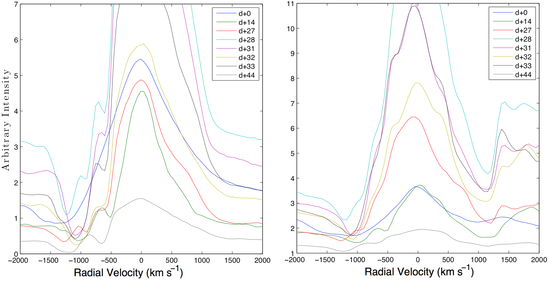
Figure 13: Radial velocities of the flat-top-jitter epoch spectra from H$\beta$ on the left and O i on the right.

References

- Anupama (2012) Anupama, G. C. 2012, in Astronomical Society of India Conference Series, Vol. 6, Astronomical Society of India Conference Series, ed. P. Prugniel & H. P. Singh, 143
- Banerjee et al. (2015) Banerjee, D. P. K., Srivastava, M., & Ashok, N. M. 2015, Atel, 7265
- Banerjee et al. (2016) Banerjee, D. P. K., Srivastava, M. K., Ashok, N. M., & Venkataraman, V. 2016, MNRAS, 455, L109
- Barnsley et al. (2012) Barnsley, R. M., Smith, R. J., & Steele, I. A. 2012, AN, 333, 101
- Basu et al. (2010) Basu, B., Chattopadhyay, T., & Biswas, S. N. 2010, An Introduction to Astrophysics, 2nd edn. (PHI Learning Pvt. Ltd)
- Cheung et al. (2016) Cheung, C. C., Jean, P., Shore, S. N., et al. 2016, ApJ, 826, 142
- Darnley et al. (2012) Darnley, M. J., Ribeiro, V. A. R. M., Bode, M. F., Hounsell, R. A., & Williams, R. P. 2012, ApJ, 746, 61
- Derdzinski et al. (2017) Derdzinski, A. M., Metzger, B. D., & Lazzati, D. 2017, MNRAS, 469, 1314
- Evans et al. (2017) Evans, A., Banerjee, D. P. K., Gehrz, R. D., et al. 2017, MNRAS, 466, 4221
- Evans et al. (2014) Evans, A., Gehrz, R. D., & Helton, L. A. 2014, MNRAS, 444, 1683
- Evans et al. (2002) Evans, A., Yudin, R. V., Naylor, T., Ringwald, F. A., & Koch Miramond, L. 2002, A&A, 384, 504
- Ferland et al. (2013) Ferland, G. J., Porter, R. L., van Hoof, P. A. M., et al. 2013, RMxAA, 49, 1
- Finzell et al. (2017) Finzell, T., Chomiuk, L., Metzger, B. D., et al. 2017, ArXiv e-prints, 1701.03094
- Fowler (1920) Fowler, A. 1920, MNRAS, 80, 692
- Gehrz et al. (2015) Gehrz, R. D., Evans, A., Woodward, C. E., et al. 2015, Atel, 7862
- Grigorian & Vardanian (1961) Grigorian, V. A. & Vardanian, R. A. 1961, Soobsh. Byurakan Obs., 29, 39
- Henze et al. (2014) Henze, M., Ness, J.-U., Darnley, M. J., et al. 2014, A&A, 563, L8
- Jack et al. (2017) Jack, D., Robles Pérez, J. d. J., De Gennaro Aquino, I., et al. 2017, Astron. Nastrich, 338, 91
- Kasliwal (2011) Kasliwal, M. M. 2011, PhD thesis, California Institute of Technology
- Kato et al. (2009) Kato, T., Nakajima, K., Maehara, H., & Kiyota, S. 2009, Variable Star Bulletin, 49
- Kemp et al. (1974) Kemp, J. C., Swedlund, J. B., & Wolstencroft, R. D. 1974, ApJL, 193, L15
- Kosenkov et al. (2017) Kosenkov, I. A., Berdyugin, A. V., Piirola, V., et al. 2017, MNRAS, 468, 4362
- Landi et al. (2008) Landi, R., Bassani, L., Dean, A., et al. 2008, MNRAS, 392, 630
- Lynch et al. (2008) Lynch, D. K., Woodward, C. E., Gehrz, R., et al. 2008, AJ, 136, 1815
- McClintock et al. (1975) McClintock, J. E., Canizares, C. R., & Tarter, C. B. 1975, ApJ, 198, 641
- McLaughlin (1942) McLaughlin, D. B. 1942, ApJ, 95, 428
- McLaughlin (1955) McLaughlin, D. B. 1955, ApJ, 122, 417
- Metzger et al. (2014) Metzger, B. D., Hascoët, R., Vurm, I., et al. 2014, MNRAS, 442, 713
- Morisset (2013) Morisset, C. 2013, Astrophysics Source Code Library, 1304.020
- Muneer et al. (2015) Muneer, S., Anupama, G. C., Raveendran, A. V., Muniyandi, A., & Baskar, R. 2015, ATel, 7310
- Nussbaumer & Storey (1984) Nussbaumer, H. & Storey, P. J. 1984, AAPS, 56, 293
- Oke (1990) Oke, J. 1990, AJ, 99, 1621
- Page et al. (2015) Page, K. L., Kuin, N. P., Osborne, J. P., & Schwarz, G. J. 2015, Atel, 7953
- Penning et al. (1986) Penning, W. R., Schmidt, G. D., & Liebert, J. 1986, ApJ, 301, 881
- Piirola et al. (2014) Piirola, V., Berdyugin, A., & Berdyugina, S. 2014, in PROCSPIE, Vol. 9147, Ground-based and Airborne Instrumentation for Astronomy V, 10.1117/12.2055923, 91478I
- Schwarz et al. (2011) Schwarz, G. J., Ness, J.-U., Osborne, J. P., et al. 2011, ApJ, 197, 26
- Seach (2015) Seach, J. 2015, CBET, 4081
- Shen et al. (2017) Shen, V., Siderius, D., Krekelberg, W., & Hatch, H. 2017, National Institute of Standards and Technology, Gaithersburg MD, 20899
- Shore (2012) Shore, S. 2012, Bull. Astr. Soc. India, 40, 28
- Steele et al. (2006) Steele, I. A., Bates, S. D., Carter, D., et al. 2006, in ProcSPIE, Vol. 6269, Society of Photo-Optical Instrumentation Engineers (SPIE) Conference Series, 62695M
- Steele et al. (2004) Steele, I. A., Smith, R. J., Rees, P. C., et al. 2004, in Proc. SPIE, Vol. 5489, Ground-based Telescopes, ed. J. M. Oschmann, Jr., 679–692
- Steffen & Lopez (2006) Steffen, W. & Lopez, J. A. 2006, RMxAA, 42, 99
- Storey et al. (2017) Storey, P., Sochi, T., & Bastin, R. 2017, ArXiv e-prints, 1703.09982
- Stratton & Manning (1939) Stratton, F. J. M. & Manning, W. H. 1939, Cambridge University Press, Cambridge: England, Solar Physics Observatory, 1939
- Strope et al. (2010) Strope, R. J., Schaefer, B. E., & Henden, A. A. 2010, AJ, 140, 34
- Swedlund et al. (1974) Swedlund, J. B., Kemp, J. C., & Wolstencroft, R. D. 1974, ApJL, 193, L11
- Tody (1993) Tody, D. 1993, in Astronomical Data Analysis Software and Systems II, ed. R. J. Hanisch, R. J. V. Brissenden, & J. Barnes, Vol. 52, 173
- Vogel (1893) Vogel, H. C. 1893, AstAp, 12, 896V
- Walker (1954) Walker, M. F. 1954, PASP, 66, 230
- Walter (2015) Walter, F. M. 2015, Atel, 7643
- Warner (1995) Warner, B. 1995, Cataclysmic Variable stars (Cambridge University Press)
- Williams (1994) Williams, R. E. 1994, ApJ, 426, 279
- Williams et al. (1991) Williams, R. E., Hamuy, M., Phillips, M. M., et al. 1991, ApJ, 376, 721
- Williams et al. (1994) Williams, R. E., Phillips, M. M., & Hamuy, M. 1994, ApSS, 90, 297
- Williams et al. (2013) Williams, S. C., Bode, M. F., Darnley, M. J., et al. 2013, ApJL, 777, L32, 4pp
- Williams et al. (2015) Williams, S. C., Darnley, M. J., & Bode, M. F. 2015, Atel, 7230
- Wright (1921) Wright, W. H. 1921, MNRAS, 81, 181
- Yaron et al. (2005) Yaron, O., Prialnik, D., Shara, M. M., & Kovetz, A. 2005, ApJ, 623, 398
- Zemko et al. (2016) Zemko, P., Orio, M., Mukai, K., et al. 2016, MNRAS, 460, 2744