Robust multigrid solvers for the biharmonic problem in isogeometric analysis

Abstract

In this paper, we develop multigrid solvers for the biharmonic problem in the framework of isogeometric analysis (IgA). In this framework, one typically sets up B-splines on the unit square or cube and transforms them to the domain of interest by a global smooth geometry function. With this approach, it is feasible to set up $H^{2}$-conforming discretizations. We propose two multigrid methods for such a discretization, one based on Gauss Seidel smoothing and one based on mass smoothing. We prove that both are robust in the grid size, the latter is also robust in the spline degree. Numerical experiments illustrate the convergence theory and indicate the efficiency of the proposed multigrid approaches, particularly of a hybrid approach combining both smoothers.

1 Introduction

Isogeometric analysis (IgA) was introduced around a decade ago as a new paradigm to the discretization of partial differential equations (PDEs) and has gained increasing attention (cf. [1] for the original paper and [2] for a survey paper). The idea of IgA – from the technical point of view – is to use B-spline spaces or similar spaces, like NURBS spaces, to discretize the problem.

In contrast to standard $C^{0}$-smooth high-order finite elements, the introduction of discretizations with higher smoothness on general computational domains is not straight forward. In IgA, splines are first set up on the unit square or the unit cube, which is usually called the parameter domain. Then, a global smooth geometry transformation mapping from the parameter domain to the physical domain, i.e., the domain of interest, is used to define the ansatz functions on the physical domain.

Such an approach allows to construct arbitrarily smooth ansatz functions. So, we easily obtain $H^{2}$-conforming discretizations which can be used as conforming discretizations of the biharmonic problem, which is for example of interest in plate theory (cf. [3]), Stokes streamline equations (cf. [4]), or Schur complement preconditioners (cf. [5, 6]). For the latter, also the three dimensional version of the biharmonic problem is of interest. Such $H^{2}$-conforming discretizations are hard to realize in a standard finite element scheme. One option is the Bogner-Fox-Schmit element, which requires a rectangular mesh, another option is the Argyris elements for triangular meshes. For such $H^{2}$-conforming elements, besides various kinds of other preconditioners (cf. [7] and references therein), also multigrid solvers have been proposed (cf. [8]). As alternative, multigrid solvers for various kinds of mixed or non-conforming formulations have been developed (cf. [9, 10, 11] and references therein).

In this paper, we develop iterative solvers for conforming Galerkin discretizations of the biharmonic problem in an isogeometric setting. Multigrid methods are known to solve linear systems arising from the discretization of partial differential equations with optimal complexity, i.e., their computational complexity grows typically only linearly with the number of unknowns. In an isogeometric setting, multigrid and multilevel methods have been discussed within the last years (cf. [12, 13, 14, 15, 16]). It was observed that multigrid methods based on standard smoothers, like the Gauss Seidel smoother, show robustness in the grid size within the isogeometric setting, their convergence rates however deteriorate significantly if the spline degree is increased. This motivated the recent publications [15, 16]. In the latter, a subspace corrected mass smoother was introduced, based on the approximation error estimates and inverse inequalities from [17].

The present paper is a continuation of [17] and [16]. We propose two multigrid methods for the linear system resulting from the discretization of the biharmonic problem, one based on Gauss Seidel smoothing and one based on a subspace corrected mass smoother. We prove that both are robust in the grid size, the latter is also robust in the spline degree. For this purpose, non-trivial extensions to both previous papers are required. [17] covers the approximation with functions whose odd derivatives vanish on the boundary; an extension to functions whose even derivatives (including the function value itself) vanish on the boundary might be straight-forward, however, for the first biharmonic problem we need a combination of both. A straight-forward extension of [16] would require full $H^{4}$ regularity, which cannot even be assumed on the unit square (cf. [18]). So, we only require partial regularity (Assumption 2) and derive the convergence results using Hilbert space interpolation.

We give numerical experiments both for domains described by trivial and non-trivial geometry transformation in two and three dimensions. We observe that the subspace corrected mass smoother outperforms the Gauss Seidel smoother for significant large spline degrees. The negative effects of the geometry transformation to the subspace corrected mass smoother, which have also been observed for the Poisson problem, are amplified in case of the biharmonic problem. Approaches to master these effects are of particular interest for the biharmonic problem. We propose a hybrid smoother which combines the strengths of both proposed smoothers and works well in our numerical experiments (cf. Section 6.3).

The remainder of the paper is organized as follows. We introduce the model problem and its discretization in Section 2. Then, in Section 3, we develop the required approximation error estimates. In Section 4, we set up a stable splitting of the spline spaces. In Section 5, we introduce the multigrid algorithms and prove their convergence. Finally, in Section 6, we give results from the numerical experiments and draw conclusions.

2 Preliminaries

2.1 Model problem

In this paper, we consider the first biharmonic problem as model problem, which reads as follows. For a given domain $\Omega\subset\mathbb{R}^{d}$ with piecewise $C^{2}$-smooth Lipschitz boundary $\Gamma=\partial\Omega$ and a given source function $f$, find the unknown function $u$ such that

$$\Delta^{2}u =f\quad\text{in}\quad\Omega,$$

$$u =0\quad\text{on}\quad\Gamma,$$ (1)

$$\nabla u\cdot\mathbf{n} =0\quad\text{on}\quad\Gamma,$$

where $\mathbf{n}$ is the outer normal vector; for simplicity, we restrict ourselves to homogenous boundary conditions. Our proposed solver can be extended to other boundary conditions, namely to the second and the third biharmonic problem, cf. Remarks 2 and 3.

Following the principle of IgA, we assume that the computational domain $\Omega$ is represented by a bijective geometry transformation

$$\mathbf{G}:\widehat{\Omega}\rightarrow\Omega$$ (2)

mapping from the parameter domain $\widehat{\Omega}:=(0,1)^{d}$ to the physical domain $\Omega$.

The variational formulation of model problem (1) is as follows.

Problem 1.

Given $f\in L^{2}\left(\Omega\right)$, find $u\in V:=H^{2}_{0}\left(\Omega\right)$ such that

$$\underbrace{\left(\Delta u,\Delta v\right)_{L^{2}\left(\Omega\right)}}_{\displaystyle\left(u,v\right)_{\mathcal{B}(\Omega)}:=}=\left(f,v\right)_{L^{2}\left(\Omega\right)}\quad\forall\,v\in V.$$ (3)

Here and in what follows, $L^{2}$ and $H^{r}$ denote the standard Lebesgue and Sobolev spaces with standard inner products $(\cdot,\cdot)_{L^{2}}$, $(\cdot,\cdot)_{H^{r}}$, norms $\|\cdot\|_{L^{2}}$, $\|\cdot\|_{H^{r}}$ and seminorms $|\cdot|_{H^{r}}=(\cdot,\cdot)_{H^{r}}^{1/2}$. $H^{2}_{0}\left(\Omega\right)$ is the standard subspace of $H^{2}$, containing the functions where the values and the derivatives vanish on the boundary, i.e.,

$$H^{2}_{0}\left(\Omega\right)=\left\{v\in H^{2}\left(\Omega\right)|\,v=\nabla v\cdot n=0\text{ on }\Gamma\right\}.$$

Note that the inner products $(\cdot,\cdot)_{H^{2}(\Omega)}$ and $\left(\cdot,\cdot\right)_{\mathcal{B}(\Omega)}$ coincide on $H^{2}_{0}\left(\Omega\right)$ (cf. [19]), i.e.,

$$\left(u,v\right)_{\mathcal{B}(\Omega)}=(u,v)_{H^{2}(\Omega)}\qquad\forall u,v\in H^{2}_{0}(\Omega).$$ (4)

Let $\left(\cdot,\cdot\right)_{\bar{\mathcal{B}}(\Omega)}$ be the inner product obtained by removing the cross terms from the inner product $\left(\cdot,\cdot\right)_{\mathcal{B}(\Omega)}$, i.e.,

$$\left(u,v\right)_{\bar{\mathcal{B}}(\Omega)}:=\sum^{d}_{k=1}\left(\partial_{x_{k}x_{k}}u,\partial_{x_{k}x_{k}}u\right)_{L^{2}\left(\Omega\right)}.$$ (5)

Here and in what follows, $\partial_{x}:=\frac{\partial}{\partial x}$ and $\partial_{xy}:=\partial_{x}\partial_{y}$ and $\partial_{x}^{r}:=\frac{\partial^{r}}{\partial x^{r}}$ denote partial derivatives.

Lemma 1.

The inner products defined in (3) and (5) are spectrally equivalent, i.e.,

$$\left(u,u\right)_{\bar{\mathcal{B}}(\Omega)}\leq\left(u,u\right)_{\mathcal{B}(\Omega)}\leq d\left(u,u\right)_{\bar{\mathcal{B}}(\Omega)}\quad\forall\,u\in H^{2}_{0}(\Omega).$$

Proof.

Using the Cauchy-Schwarz inequality and $ab\leq\tfrac{1}{2}(a^{2}+b^{2})$, we obtain

$$\|u\|_{\mathcal{B}(\Omega)}^{2} =\sum_{k=1}^{d}\sum_{l=1}^{d}\left(\partial_{x_{k}x_{k}}u,\partial_{x_{l}x_{l}}u\right)_{L^{2}\left(\Omega\right)}$$

$$\leq\frac{1}{2}\sum_{k=1}^{d}\sum_{l=1}^{d}\left(\left\|\partial_{x_{k}x_{k}}u\right\|_{L^{2}\left(\Omega\right)}^{2}+\left\|\partial_{x_{l}x_{l}}u\right\|_{L^{2}\left(\Omega\right)}^{2}\right)=d\|u\|_{\bar{\mathcal{B}}(\Omega)}^{2},$$

which shows one direction. Using the boundary conditions and (4), we obtain

$$\|u\|_{\mathcal{B}(\Omega)}^{2} =\|u\|_{H^{2}(\Omega)}^{2}=\|u\|_{\bar{\mathcal{B}}(\Omega)}^{2}+\sum_{k=1}^{d}\sum_{l\in\{1,\ldots,d\}\backslash\{k\}}\underbrace{\left(\partial_{x_{k}x_{l}}u,\partial_{x_{k}x_{l}}u\right)_{L^{2}\left(\Omega\right)}}_{\displaystyle\geq 0},$$

which shows the other direction. ∎

2.2 Spline space

We consider standard tensor product B-spines with maximum continuity (see, e.g., [20]). Let the interval $(0,1)$ be subdivided into $m\in\mathbb{N}$ elements of length $h=1/m$. The space of splines of degree $p\in\mathbb{N}:=\{1,2,3,\ldots\}$ with maximum continuity is defined by

$$S_{p,h}(0,1):=\left\{u\in C^{p-1}\left(0,1\right):u|_{\left(\left(i-1\right)h,ih\right)}\in\mathcal{P}^{p}\quad\forall\,j=1,\ldots m\right\},$$

where $C^{p-1}\left(0,1\right)$ is the space of all $p-1$ times continuously differentiable functions on $\left(0,1\right)$ and $\mathcal{P}^{p}$ is the space of all polynomials with degree at most $p$. We use the standard $B$-splines with open knot vector as basis for $S_{p,h}(0,1)$. The dimension of $S_{p,h}(0,1)$ is $n:=\dim{S_{p,h}(0,1)}=m+p$. We will from time to time omit the subscripts $p$ and $h$ of a spline space $S_{p,h}(0,1)$ and write $S(0,1)$ or just $S$. For higher dimensions $d>1$, we use the tensor product splines

$$S_{p,h}(\widehat{\Omega})=S_{p,h}(0,1)\otimes\ldots\otimes S_{p,h}(0,1),$$

defined over $\widehat{\Omega}=\left(0,1\right)^{d}$. For notational convenience, we assume that all of those univariate spline spaces $S_{p,h}$ have the same spline degree $p$ and the same number of elements $m$, however, this in not necessary and the results in this paper can easily be generalized to the case with different $p$ and $m$.

Based on the spline space on the parameter space, we define the spline space on the physical space using the standard pull-back principle as

$$S_{p,h}(\Omega)=\{u\;:\;u\circ\mathbf{G}\in S_{p,h}(\widehat{\Omega})\},$$

where $\mathbf{G}$ is the geometry transformation (2). We assume that the geometry transformation is sufficiently smooth such that the following estimate holds.

Assumption 1.

Assume that there exist constants $\underline{\alpha}>0$ and $\overline{\alpha}$ such that

$$\underline{\alpha}\,\|u\|_{H^{q}(\Omega)}\leq\|u\circ\mathbf{G}\|_{H^{q}(\widehat{\Omega})}\leq\overline{\alpha}\,\|u\|_{H^{q}(\Omega)}\quad\forall\,u\in H^{q}(\Omega),\,q\in\{2,3\}.$$

We discretize the Problem 1 using the Galerkin principle as follows.

Problem 2.

Given $f\in L^{2}(\Omega)$, find $u\in V_{h}:=S_{p,h}^{0}(\Omega):=H^{2}_{0}\left(\Omega\right)\cap S_{p,h}(\Omega)$ such that

$$\left(u,v\right)_{\mathcal{B}(\Omega)}=\left(f,v\right)_{L^{2}\left(\Omega\right)}\quad\forall\,v\in V_{h}.$$ (6)

By fixing a basis for the space $S_{p,h}^{0}(\Omega)$, we can rewrite the Problem 2 in matrix-vector notation as

$$\mathcal{B}_{h}u_{h}=f_{h},$$ (7)

where $\mathcal{B}_{h}$ is a standard stiffness matrix, $u_{h}$ is the representation of the corresponding function $u$ with respect to the chosen basis and the vector $f_{h}$ is obtained by testing the right hand side functional $(f,\cdot)_{L^{2}(\Omega)}$ with the basis functions.

For convenience, we use the following notation.

Notation 1.

Throughout this paper, $c$ is a generic positive constant independent of $h$ and $p$, but may depend on $d$ and $\mathbf{G}$.

2.3 Regularity

In the following sections, we use Aubin-Nitsche duality arguments for showing the desired error estimates. This requires that the following assumption holds.

Assumption 2.

For a given $f\in H^{-1}(\Omega)$, the solution $u\in H^{2}_{0}\left(\Omega\right)$ of the first biharmonic problem (1) satisfies

$$u\in H^{3}(\Omega)\qquad\mbox{and}\qquad\|u\|_{H^{3}(\Omega)}\leq c\|f\|_{H^{-1}(\Omega)}.$$

Such a result is satisfied for convex polygonal domains (cf. [18]). It is worth noting that this implies that the result also holds for the parameter domain $\widehat{\Omega}=(0,1)^{2}$.

As we only rely on a partial regularity result, we use Hilbert space interpolation (cf. [21, 22]) to derive our estimates. defined, e.g., with the K-method, is a Hilbert space with norm $\|\cdot\|_{[A_{1},A_{2}]_{\theta}}.$ Applied to Sobolev spaces $H^{m}(\Omega)$ and $H^{n}(\Omega)$, we obtain

$$\|\cdot\|_{[H^{m}(\Omega),H^{n}(\Omega)]_{\theta}}^{2}=\|\cdot\|_{H^{(1-\theta)m+\theta n}(\Omega)}^{2},$$ (8)

see [21, Theorem 6.4.5], applied to scaled Hilbert spaces $A_{1}$ and $\gamma A_{2}$ with a scaling parameter $\gamma>0$, we obtain

$$\|\cdot\|_{[A_{1},\gamma A_{2}]_{\theta}}^{2}=\gamma^{\theta}\|\cdot\|_{[A_{1},A_{2}]_{\theta}}^{2}$$ (9)

and applied to the intersections of two Hilbert spaces $A_{1}\cap A_{2}$ with norm ${\|\cdot\|_{A_{1}\cap A_{2}}^{2}:=\|\cdot\|_{A_{1}}^{2}+\|\cdot\|_{A_{2}}^{2}}$, we obtain

$$\|\cdot\|_{[A_{1},A_{1}\cap A_{2}]_{\theta}}^{2}\leq c\|\cdot\|_{A_{1}\cap[A_{1},A_{2}]_{\theta}}^{2},$$ (10)

see [23, Lemma 6.1], and applied to dual norms, we obtain

$$\|\cdot\|_{([A_{1},A_{2}]_{\theta})^{\prime}}^{2}=\|\cdot\|_{[A_{1}^{\prime},A_{2}^{\prime}]_{\theta}}^{2},$$ (11)

see [21, Theorem 3.7.1]. As the interpolation defined by the K-method is an exact interpolation function, see [21, Theorem 3.1.2], we know that any bounded operator $\Psi$, which maps from a Hilbert space $A_{1}$ to a Hilbert space $B_{1}$ and from a Hilbert space $A_{2}$ to a Hilbert space $B_{2}$, maps also from $[A_{1},A_{2}]_{\theta}$ to $[B_{1},B_{2}]_{\theta}$ and satisfies

$$\|\Psi a\|_{[B_{1},B_{2}]_{\theta}}\leq cM_{1}^{1-\theta}M_{2}^{\theta}\|a\|_{[A_{1},A_{2}]_{\theta}}\qquad\mbox{with}\quad M_{i}:=\sup_{a_{i}\in A_{i}}\frac{\|\Psi a_{i}\|_{B_{i}}}{\|a_{i}\|_{A_{i}}}$$ (12)

for all $\theta\in(0,1)$, where $c$ only depends on $\theta$.

3 Approximation error estimates

One vital component needed to prove multigrid convergence is an approximation error estimate. Approximation error estimates between the spaces $L^{2}\left(\Omega\right)$ and $H^{1}\left(\Omega\right)$ are given in [17, 24] and used in [15, 16] to prove convergence for a multigrid solver for the Poisson problem. For the biharmonic problem we need similar estimates for $H^{2}\left(\Omega\right)$.

3.1 Approximation error estimates for the periodic case

We start the analysis for the periodic case. We define for each $q\in\mathbb{N}$ the periodic Sobolev space

$$H^{q}_{per}(-1,1):=\left\{u\in H^{q}(-1,1)\,:\,u^{\left(l\right)}\left(-1\right)=u^{\left(l\right)}\left(1\right),\quad\forall\,l\in\mathbb{N}_{0}\mbox{ with }l<q\right\}$$

and for each $p\in\mathbb{N}$ the periodic spline space

$$S_{p,h}^{per}(-1,1):=\left\{u\in S(-1,1)\,:\,u^{\left(l\right)}\left(-1\right)=u^{\left(l\right)}\left(1\right)\quad\forall\,l\in\mathbb{N}_{0}\mbox{ with }l<p\right\}.$$

Let $T_{p,h}^{q,per}$ be the $H^{q,\circ}$-orthogonal projection into $S_{p,h}^{per}(-1,1)$, where the underlying scalar product $\left(\cdot,\cdot\right)_{H^{q,\circ}(-1,1)}$ is given by

$$\left(u,v\right)_{H^{r,\circ}(-1,1)}:=\left\{\begin{array}[]{ll}\left(u,v\right)_{H^{q}(-1,1)}+\frac{1}{2}\int^{1}_{-1}u\,\text{d}x\int^{1}_{-1}v\,\text{d}x&\;\text{ for }\;q>0,\\ \left(u,v\right)_{L^{2}(-1,1)}&\;\text{ for }\;q=0,\end{array}\right.$$

where $\frac{1}{2}\int^{1}_{-1}u\,\text{d}x\int^{1}_{-1}v\,\text{d}x$ is added to enforce uniqueness.

Theorem 1.

Let $p\in\mathbb{N}_{0}$, $q\in\mathbb{N}_{0}$ with $p\geq q$ and $hp<1$. Then,

$$|(I-T_{p,h}^{q,per})u|_{H^{q}(-1,1)}\leq\sqrt{2}h|u|_{H^{q+1}(-1,1)}\quad\forall u\in H^{q+1}_{per}(-1,1).$$

Proof.

We use induction with respect to $q$.

Proof for $q=0$. [17, Lemma 4.1] gives an approximation error estimate for the $H^{1,\circ}$-orthogonal projection of $u$ into $S_{p,h}^{per}$ for $p\geq 1$. Because $T_{p,h}^{0,per}$ minimizes the $L^{2}$-norm, we obtain

$$\|(I-T_{p,h}^{0,per})u\|_{L^{2}}\leq\|(I-T_{p,h}^{1,per})u\|_{L^{2}}\leq\sqrt{2}h|u|_{H^{1}}\quad\forall\,u\in H^{1}_{per}(-1,1),$$

i.e., the desired result. For $p=0$, we observe that there are no periodicity conditions for the space $S_{p,h}^{per}$. The desired result on approximation by piecewise constants is standard and can be found, e.g, in [25, Theorem 6.1].

Proof for $q>0$. We already know that the induction hypothesis holds true for $q-1$, i.e., we have

$$|u-T_{p-1,h}^{q-1,per}u|_{H^{q-1}(-1,1)}\leq\sqrt{2}h|u|_{H^{q}(-1,1)}\quad\forall\,u\in H^{q}_{per}(-1,1).$$ (13)

As a next step we show that for all $u\in H^{q+1}_{per}(-1,1)$, there is a $u_{h}\in S_{p,h}^{per}$ such that

$$|u-u_{h}|_{H^{q}(-1,1)}\leq\sqrt{2}h|u|_{H^{q+1}(-1,1)}.$$ (14)

By plugging $u^{\prime}$ into (13), we immediately obtain

$$|u^{\prime}-T_{p-1,h}^{q-1,per}u^{\prime}|_{H^{q-1}(-1,1)}\leq\sqrt{2}h|u|_{H^{q+1}(-1,1)}\quad\forall\,u\in H^{q+1}_{per}(-1,1).$$

Let $v_{h}:=T_{p-1,h}^{q-1,per}u^{\prime}$ and define $u_{h}(x):=\int_{-1}^{x}v_{h}(\xi)\text{d}\xi+\gamma$, where $\gamma\in\mathbb{R}$ such that $\int_{-1}^{1}u_{h}(x)\text{d}x=0$. For this choice, we obtain the desired estimate (14). It remains to show $u_{h}\in S_{p,h}^{per}$. As we have $v_{h}\in S_{p-1,h}^{per}$, we obtain that $u_{h}$ is a spline of degree $p$. The continuity estimates

$$u_{h}^{(l)}(-1)=u_{h}^{(l)}(1)\quad\mbox{for }l=1,\ldots,p-1$$

follow directly from $v_{h}^{(l)}(-1)=v_{h}^{(l)}(1)\quad\mbox{for }l=0,\ldots,p-2$. So, it remains to show $u_{h}(-1)=u_{h}(1)$. Note that, as $u$ is periodic, we have

$$u_{h}(-1)-u_{h}(1) =(u(1)-u(-1))-(u_{h}(1)-u_{h}(-1))=\int_{-1}^{1}u^{\prime}(x)-u_{h}^{\prime}(x)\text{d}x$$

$$=\int_{-1}^{1}v(x)-v_{h}(x)\text{d}x=((I-T_{p-1,h}^{q-1,per})v,1)_{L^{2}(-1,1)}.$$

Note that $(\cdot,1)_{H^{r,\circ}(-1,1)}=(\cdot,1)_{L^{2}(-1,1)}$ for any $r$, so we obtain

$$u_{h}(-1)-u_{h}(1)=((I-T_{p-1,h}^{q-1,per})v,1)_{H^{q-1,\circ}(-1,1)}$$

and finally, as $1\in S_{p-1,h}^{per}$, Galerkin orthogonality shows that this term is $0$. So, we have shown $u_{h}\in S_{p,h}^{per}$ and (14). As the projector $T_{p,h}^{q,per}$ minimizes the $H^{q}$-seminorm, we obtain

$$|(I-T_{p,h}^{q,per})u|_{H^{q}(-1,1)}\leq|u-u_{h}|_{H^{q}(-1,1)}\leq\sqrt{2}h|u|_{H^{q+1}(-1,1)},$$

i.e., the desired result. ∎

3.2 Approximation error estimates for the univariate case

Now, we derive approximation error estimates for univariate splines that satisfy the desired boundary conditions. First, we consider the approximation of functions in the Sobolev space of functions with vanishing even derivatives (and function values) on the boundary, given by

$$H^{q}_{D}(0,1):=\left\{u\in H^{q}(0,1)\,:\,u^{\left(2l\right)}\left(0\right)=u^{\left(2l\right)}\left(1\right)=0,\quad\forall\,l\in\mathbb{N}_{0}\text{ with }2l<q\right\},$$

by functions in a corresponding spline space, given by

$$S^{D,0}(0,1):=\left\{u\in S(0,1):u^{\left(2l\right)}\left(0\right)=u^{\left(2l\right)}\left(1\right)=0\quad\forall\,l\in\mathbb{N}_{0}\text{ with }2l<p\right\}.$$

Now, we define $\Pi^{D,0}$ to be the $H^{2}$-orthogonal projection from $H^{2}_{D}(0,1)$ into $S^{D,0}(0,1)$. This projector satisfies the following error estimate.

Theorem 2.

Let $p\in\mathbb{N}$ with $p\geq 3$ and $hp<1$. Then,

$$|(I-\Pi^{D,0})u|_{H^{2}(0,1)}\leq 2h^{2}|u|_{H^{4}(0,1)}\quad\forall u\in H^{4}_{D}(0,1)$$

Proof.

Assume $u\in H^{4}_{D}(0,1)$ to be arbitrary but fixed. Define $w$ on $(-1,1)$ by

$$w(x):=\mbox{sign}(x)\,u(|x|)$$

and observe that $w\in H^{4}_{per}(-1,1)$. Using Theorem 1, we obtain

$$|(I-T_{p,h}^{2,per})w|_{H^{2}(-1,1)} =|(I-T_{p,h}^{2,per})(I-T_{p,h}^{3,per})w|_{H^{2}(-1,1)}$$

$$\leq\sqrt{2}h|(I-T_{p,h}^{3,per})w|_{H^{3}(-1,1)}\leq{2}h^{2}|w|_{H^{4}(-1,1)}.$$

First observe that $|w|_{H^{4}(-1,1)}=\sqrt{2}|u|_{H^{4}(0,1)}$. Define $w_{h}:=T_{p,h}^{2,per}w$ and observe that we obtain $w_{h}(x)=-w_{h}(-x)$ using a standard symmetry argument. This implies that $u_{h}$, the restriction of $w_{h}$ to $(0,1)$, satisfies $u_{h}\in S^{D,0}$. Moreover, we have $|w-w_{h}|_{H^{2}(-1,1)}=\sqrt{2}|u-u_{h}|_{H^{2}(0,1)}$ and, as a consequence,

$$|u-u_{h}|_{H^{2}(0,1)}\leq 2h^{2}|u|_{H^{4}(0,1)}.$$

As the projector $\Pi^{D,0}$ minimizes the $H^{2}$-seminorm, the desired result follows. ∎

Now, we consider the boundary conditions of interest for the first biharmonic problem. Here, the continuous space is $H^{2}_{0}(0,1)$ and the discretized space is $S^{0}(0,1)$, given by

$$S^{0}(0,1):=\left\{u\in S(0,1)\,:\,u(0)=u^{\prime}(0)=u(1)=u^{\prime}(1)=0\right\}=S(0,1)\cap H^{2}_{0}(0,1).$$

Now, we define $\Pi^{0}$ to be the $H^{2}$-orthogonal projection from $H^{2}_{0}(0,1)$ into $S^{0}(0,1)$. This projector satisfies the following error estimate.

Theorem 3.

Let $p\in\mathbb{N}$ with $p\geq 3$ and $hp<1$. Then,

$$|(I-\Pi^{0})u|_{H^{2}(0,1)}\leq 2h^{2}|u|_{H^{4}(0,1)}\quad\forall\,u\in H^{4}(0,1)\cap H^{2}_{0}(0,1).$$

Proof.

First, define $S^{*}(0,1):=S\cap H^{1}_{0}(0,1)$ and $\Pi^{*}:H^{2}_{D}(0,1)\rightarrow S^{*}$ to be the $H^{2}$-orthogonal projector into the corresponding space. Since $S^{D,0}\subset S^{*}$, Theorem 2 directly implies

$$|\left(I-\Pi^{*}\right)w|_{H^{2}(0,1)}\leq 2h^{2}|w|_{H^{4}(0,1)}\quad\forall\,w\in H^{4}_{D}(0,1).$$

Now let $u\in H^{4}(0,1)\cap H^{1}_{0}(0,1)$ be arbitrary but fixed. Observe that for

$$w(x):=u(x)+\underbrace{\frac{1}{6}(x^{3}-3x^{2}+2x)}_{\displaystyle\phi_{1}(x):=}u^{\prime\prime}(0)-\underbrace{\frac{1}{6}(x^{3}-x)}_{\displaystyle\phi_{2}(x):=}u^{\prime\prime}(1),$$

we obtain $w\in H^{4}_{D}(0,1)$. Note that $\phi_{1},\phi_{2}\in S^{*}$ and $|\phi_{1}|_{H^{4}(0,1)}=|\phi_{2}|_{H^{4}(0,1)}=0$. So,

$$|\left(I-\Pi^{*}\right)u|_{H^{2}(0,1)} =\inf_{u^{*}\in S^{*}}|u-u^{*}|_{H^{2}(0,1)}$$

$$=\inf_{w^{*}\in S^{*}}|w-w^{*}|_{H^{2}(0,1)}\leq 2h^{2}|w|_{H^{4}(0,1)}=2h^{2}|u|_{H^{4}(0,1)}.$$

Now, consider the function $\psi_{1}(x):=\tfrac{1}{2}(x^{2}-x)$ and observe $\psi_{1}\in S^{*}$ and

$$0=(\left(I-\Pi^{*}\right)u,\psi_{1})_{H^{2}(0,1)}=[\left(I-\Pi^{*}\right)u]^{\prime}(1)-[\left(I-\Pi^{*}\right)u]^{\prime}(0).$$ (15)

As $\left(I-\Pi^{*}\right)u\in H^{1}_{0}$, we obtain

$$0=[\left(I-\Pi^{*}\right)u](1)-[\left(I-\Pi^{*}\right)u](0)=(\left(I-\Pi^{*}\right)u,\psi_{2}^{\prime\prime})_{H^{1}(0,1)},$$

where $\psi_{2}(x):=\frac{1}{6}(x^{3}-x)$. Integration by parts and $\psi_{2}^{\prime\prime}(0)=0$ yields

$$0=(\left(I-\Pi^{*}\right)u,\psi_{2}^{\prime\prime})_{H^{1}(0,1)}=-(\left(I-\Pi^{*}\right)u,\psi_{2})_{H^{2}(0,1)}+[[\left(I-\Pi^{*}\right)u]^{\prime}\psi_{2}^{\prime\prime}](1).$$

As $\psi_{2}\in S^{*}$, Galerkin orthogonality yields $-(\left(I-\Pi^{*}\right)u,\psi_{2})_{H^{2}(0,1)}=0$, so we have $[\left(I-\Pi^{*}\right)u]^{\prime}(1)=0$. This implies, in combination with (15), that

$$u^{\prime}(1)=(\Pi^{*}u)^{\prime}(1)\quad\mbox{and}\quad u^{\prime}(0)=(\Pi^{*}u)^{\prime}(0)$$

holds. So, for any $u\in H^{2}_{0}(0,1)$, we have $\Pi^{*}u\in S^{*}\cap H^{2}_{0}=S^{0}$. As $\Pi^{0}$ minimizes the same norm, we obtain for any $u\in H^{2}_{0}(0,1)$ that $\Pi^{*}u=\Pi^{0}u$, so also the projector $\Pi^{0}$ satisfies the desired error estimate. ∎

Theorem 4.

Let $p\in\mathbb{N}$ with $p\geq 3$ and $hp<1$. Then,

$$\|(I-\Pi^{0})u\|_{L^{2}(0,1)}\leq 2h^{2}|u|_{H^{2}(0,1)}\quad\forall\,u\in H^{2}_{0}(0,1).$$

Proof.

This is shown using a classical Aubin Nitsche duality trick. Let $u\in H^{2}_{0}(0,1)$ be arbitrary but fixed and choose $v\in H^{4}(0,1)\cap H^{2}_{0}(0,1)$ such that $v^{\prime\prime\prime\prime}=u-\Pi^{0}u$. Using integration by parts and Theorem 3, we obtain

$$\|u-\Pi^{0}u\|_{L^{2}(0,1)} =\frac{\left(u-\Pi^{0}u,u-\Pi^{0}u\right)_{L^{2}(0,1)}}{|u-\Pi^{0}u|_{L^{2}(0,1)}}=\frac{\left(u-\Pi^{0}u,v^{\prime\prime\prime\prime}\right)_{L^{2}(0,1)}}{|v|_{H^{4}(0,1)}}$$

$$=\frac{\left(u-\Pi^{0}u,v\right)_{H^{2}(0,1)}}{|v|_{H^{4}(0,1)}}\leq 2\,h^{2}\frac{\left(u-\Pi^{0}u,v\right)_{H^{2}(0,1)}}{|v-\Pi^{0}v|_{H^{2}(0,1)}}.$$

Galerkin orthogonality gives $\left(u-\Pi^{0}u,\Pi^{0}v\right)_{H^{2}(0,1)}=0$. Using this, the Cauchy-Schwarz inequality and this $H^{2}$-stability of $\Pi^{0}$, we finally obtain

$$\|u-\Pi^{0}u\|_{L^{2}(0,1)} \leq 2\,h^{2}\frac{\left(u-\Pi^{0}u,v-\Pi^{0}v\right)_{H^{2}(0,1)}}{|v-\Pi^{0}v|_{H^{2}(0,1)}}$$

$$\leq 2\,h^{2}|u-\Pi^{0}u|_{H^{2}(0,1)}\leq 2\,h^{2}|u|_{H^{2}(0,1)},$$

which finishes the proof. ∎

3.3 Approximation error estimates for the parameter domain

In this subsection, we derive robust approximation error estimates for the space $S^{0}(\widehat{\Omega})$. For this purpose, we define the following projectors on $u\in H^{2}(\widehat{\Omega})$:

$$(\Pi^{x_{k}})u(x_{1},\ldots,x_{k-1},\cdot,x_{k+1},\ldots,x_{d}):=\Pi^{0}u(x_{1},\ldots,x_{k-1},\cdot,x_{k+1},\ldots,x_{d})$$

$$\hskip 73.97733pt\forall\,(x_{1},\ldots,x_{k-1},x_{k+1},\ldots,x_{d})\in(0,1)^{d-1}\quad\text{for}\quad k=1,\ldots,d.$$

Lemma 2.

The projectors $\Pi^{x_{k}}$ are commutative; that is,

$$\Pi^{x_{i}}\Pi^{x_{j}}=\Pi^{x_{j}}\Pi^{x_{i}}\quad\text{for}\quad i=1,\ldots,d\quad\text{and}\quad j=1,\ldots,d.$$

Proof.

The proof is completely analogous to that of [26, Lemma 12]. ∎

Let $\widehat{\mathbf{\Pi}}:=\widehat{\mathbf{\Pi}}_{p,h}$ be the $H^{2}$-orthogonal projection from $H^{2}_{0}(\widehat{\Omega})$ into $S^{0}(\widehat{\Omega})=S^{0}_{p,h}(\widehat{\Omega})$.

Theorem 5.

Let $p\in\mathbb{N}$ with $p\geq 3$ and $hp<1$. Then,

$$|(I-\widehat{\mathbf{\Pi}})u|_{H^{2}(\widehat{\Omega})}\leq c\,h^{2}|u|_{H^{4}(\widehat{\Omega})}\quad\forall\,u\in H^{4}(\widehat{\Omega})\cap H^{2}_{0}(\widehat{\Omega}).$$

Proof.

For sake of simplicity, we restrict the proof to the two dimensional case. Using the triangle inequality and the $H^{2}$-stability of $\Pi^{x}$, we obtain

$$\|\partial_{xx}(u-\Pi^{x}\Pi^{y}u)\|_{L^{2}(\widehat{\Omega})} \leq\|\partial_{xx}(u-\Pi^{x}u)\|_{L^{2}(\widehat{\Omega})}+\|\partial_{xx}\Pi^{x}(u-\Pi^{y}u)\|_{L^{2}(\widehat{\Omega})}$$

$$\leq\|\partial_{xx}(u-\Pi^{x}u)\|_{L^{2}(\widehat{\Omega})}+\|\partial_{xx}(u-\Pi^{y}u)\|_{L^{2}(\widehat{\Omega})}.$$

Using Theorems 3 and 4 and $a+b\leq c(a^{2}+b^{2})^{1/2}$, we obtain

$$\|\partial_{xx}(u-\Pi^{x}\Pi^{y}u)\|_{L^{2}(\widehat{\Omega})} \leq c\,h^{2}\left(\|\partial_{xxxx}u\|^{2}_{L^{2}(\widehat{\Omega})}+\|\partial_{xxyy}u\|^{2}_{L^{2}(\widehat{\Omega})}\right)^{1/2}.$$

Using Lemma 2 and the same arguments as above, we obtain

$$\|\partial_{yy}(u-\Pi^{x}\Pi^{y}u)\|_{L^{2}(\widehat{\Omega})}\leq c\,h^{2}\left(\|\partial_{yyxx}u\|^{2}_{L^{2}(\widehat{\Omega})}+\|\partial_{yyyy}u\|^{2}_{L^{2}(\widehat{\Omega})}\right)^{1/2}.$$

Using this and Lemma 1, we finally obtain

$$|(I-\widehat{\mathbf{\Pi}})u|^{2}_{H^{2}(\widehat{\Omega})}\leq|\left(I-\Pi^{x}\Pi^{y}\right)u|^{2}_{H^{2}(\widehat{\Omega})}=|\left(I-\Pi^{x}\Pi^{y}\right)u|^{2}_{\mathcal{B}(\widehat{\Omega})}$$

$$\leq 2|\left(I-\Pi^{x}\Pi^{y}\right)u|^{2}_{\bar{\mathcal{B}}(\widehat{\Omega})}=2\|\partial_{xx}(u-\Pi^{x}\Pi^{y}u)\|^{2}_{L^{2}(\widehat{\Omega})}+2\|\partial_{yy}(u-\Pi^{x}\Pi^{y}u)\|^{2}_{L^{2}(\widehat{\Omega})}$$

$$\leq c\,h^{4}\left(\|\partial_{xxxx}u\|^{2}_{L^{2}(\widehat{\Omega})}+\|\partial_{xxyy}u\|^{2}_{L^{2}(\widehat{\Omega})}+\|\partial_{yyxx}u\|^{2}_{L^{2}(\widehat{\Omega})}+\|\partial_{yyyy}u\|^{2}_{L^{2}(\widehat{\Omega})}\right)$$

$$=c\,h^{4}|u|^{2}_{H^{4}(\widehat{\Omega})}.$$

∎

Theorem 6.

Let $p\in\mathbb{N}$ with $p\geq 3$ and $hp<1$. Then,

$$|(I-\widehat{\mathbf{\Pi}})u|_{H^{2}(\widehat{\Omega})}\leq c\,h|u|_{H^{3}(\widehat{\Omega})}\quad\forall\,u\in H^{3}(\widehat{\Omega})\cap H^{2}_{0}(\widehat{\Omega}).$$

Proof.

Theorem 5 states

$$|(I-\widehat{\mathbf{\Pi}})u|_{H^{2}(\widehat{\Omega})}\leq c\,h^{2}|u|_{H^{4}(\widehat{\Omega})}\quad\forall\,u\in H^{4}(\widehat{\Omega})\cap H^{2}_{0}(\widehat{\Omega}),$$

and, as $\widehat{\mathbf{\Pi}}$ is stable in $H^{2}$, we have

$$|(I-\widehat{\mathbf{\Pi}})u|_{H^{2}(\widehat{\Omega})}\leq|u|_{H^{2}(\widehat{\Omega})}\quad\forall\,u\in H^{2}_{0}(\widehat{\Omega}),$$

Using (12) for $\theta=1/2$ and (8), we obtain the desired result. ∎

Theorem 7.

Let $p\in\mathbb{N}$ with $p\geq 3$ and $hp<1$. Then,

$$|(I-\widehat{\mathbf{\Pi}})u|_{H^{1}(\widehat{\Omega})}\leq c\,h|u|_{H^{2}(\widehat{\Omega})}\quad\forall\,u\in H^{2}_{0}(\widehat{\Omega}).$$

Proof.

This proof is a variant of the classical Aubin Nitsche duality trick. Let $u\in H^{2}_{0}(\widehat{\Omega})$ be arbitrary but fixed. Define $f\in H^{-1}(\widehat{\Omega})$ by $\langle f,\cdot\rangle:=(u-\widehat{\mathbf{\Pi}}u,\cdot)_{H^{1}(\widehat{\Omega})}$ and define $w\in H^{2}_{0}(\Omega)$ to be such that

$$(\Delta w,\Delta\widetilde{w})_{L^{2}(\widehat{\Omega})}=\langle f,\widetilde{w}\rangle\quad\forall\,\widetilde{w}\in H^{2}_{0}(\widehat{\Omega}).$$

Lax Milgram lemma yields $|w|_{H^{2}(\widehat{\Omega})}=\|f\|_{H^{-2}(\widehat{\Omega})}$. Assumption 2 (applied to the parameter domain) implies $w\in H^{3}(\widehat{\Omega})$ and $|w|_{H^{3}(\widehat{\Omega})}\leq c\|f\|_{H^{-1}(\widehat{\Omega})}=c|u-\widehat{\mathbf{\Pi}}u|_{H^{1}(\widehat{\Omega})}$. We obtain

$$|u-\widehat{\mathbf{\Pi}}u|_{H^{1}(\widehat{\Omega})}=\frac{(u-\widehat{\mathbf{\Pi}}u,u-\widehat{\mathbf{\Pi}}u)_{H^{1}(\widehat{\Omega})}}{|u-\widehat{\mathbf{\Pi}}u|_{H^{1}(\widehat{\Omega})}}\leq c\frac{(u-\widehat{\mathbf{\Pi}}u,u-\widehat{\mathbf{\Pi}}u)_{H^{1}(\widehat{\Omega})}}{|w|_{H^{3}(\widehat{\Omega})}}.$$

Using Theorem 6, we further obtain

$$|u-\widehat{\mathbf{\Pi}}u|_{H^{1}(\widehat{\Omega})}\leq ch\frac{(u-\widehat{\mathbf{\Pi}}u,u-\widehat{\mathbf{\Pi}}u)_{H^{1}(\widehat{\Omega})}}{|w-\widehat{\mathbf{\Pi}}w|_{H^{2}(\widehat{\Omega})}}.$$

The definitions of $f$ and $w$, Galerkin orthogonality, Cauchy-Schwarz inequality and the $H^{2}$-stability of $\widehat{\mathbf{\Pi}}$ yield

$$|u-\widehat{\mathbf{\Pi}}u|_{H^{1}(\widehat{\Omega})} \leq ch\frac{\langle f,u-\widehat{\mathbf{\Pi}}u\rangle}{|w-\widehat{\mathbf{\Pi}}w|_{H^{2}(\widehat{\Omega})}}=ch\frac{(\Delta w,\Delta(u-\widehat{\mathbf{\Pi}}u))_{L^{2}(\widehat{\Omega})}}{|w-\widehat{\mathbf{\Pi}}w|_{H^{2}(\widehat{\Omega})}}$$

$$\leq ch\frac{(w,u-\widehat{\mathbf{\Pi}}u)_{H^{2}(\widehat{\Omega})}}{|w-\widehat{\mathbf{\Pi}}w|_{H^{2}(\widehat{\Omega})}}=ch\frac{(w-\widehat{\mathbf{\Pi}}w,u-\widehat{\mathbf{\Pi}}u)_{H^{2}(\widehat{\Omega})}}{|w-\widehat{\mathbf{\Pi}}w|_{H^{2}(\widehat{\Omega})}}\leq ch|u-\widehat{\mathbf{\Pi}}u|_{H^{2}(\widehat{\Omega})}$$

$$\leq ch|u|_{H^{2}(\widehat{\Omega})},$$

which finishes the proof. ∎

3.4 Approximation error estimates for the physical domain

In this subsection, we extend the robust approximation error estimates for the space $S^{0}(\widehat{\Omega})$ to the space $S^{0}(\Omega)=S(\Omega)\cap H^{2}_{0}(\Omega)$. For this purpose, we define $\mathbf{\Pi}=\mathbf{\Pi}_{p,h}$ to be the $H^{2}$-orthogonal projection from $H^{2}_{0}(\Omega)$ into $S^{0}(\Omega)=S^{0}_{p,h}(\Omega)$. Here and in what follows, $h$ always refers to the grid size on the parameter domain. All estimates directly carry over to the grid size $h_{\Omega}$ on the physical domain because we have $c^{-1}h\leq h_{\Omega}\leq ch$.

Theorem 8.

Let $p\in\mathbb{N}$ with $p\geq 3$ and $hp<1$. Then,

$$|\left(I-\mathbf{\Pi}\right)u|_{H^{2}(\Omega)}\leq c\,h|u|_{H^{3}(\Omega)}\quad\forall\,u\in H^{3}(\Omega)\cap H^{2}_{0}(\Omega).$$

Proof.

Let $u\in H^{3}(\Omega)\cap H^{2}_{0}(\Omega)$ and $\widehat{u}:=u\circ\textbf{G}$. By combining Friedrichs’ inequality, Theorem 6 and Assumption 1, we obtain

$$\underline{\alpha}\,|u-[\widehat{\mathbf{\Pi}}\widehat{u}]\circ\textbf{G}^{-1}|_{H^{2}(\Omega)} \leq\|(I-\widehat{\mathbf{\Pi}})\widehat{u}\|_{H^{2}(\widehat{\Omega})}\leq c|(I-\widehat{\mathbf{\Pi}})\widehat{u}|_{H^{2}(\widehat{\Omega})}\leq c\,h|\widehat{u}|_{H^{3}(\widehat{\Omega})}$$

$$\leq\overline{\alpha}\,c\,h\|u\|_{H^{3}(\Omega)}\leq\overline{\alpha}\,c\,h|u|_{H^{3}(\Omega)},$$

where $[\widehat{\mathbf{\Pi}}\widehat{u}]\circ\textbf{G}^{-1}\in S^{0}(\Omega)$. As $\mathbf{\Pi}$ minimizes the $H^{2}$-seminorm, we obtain $|\left(I-\mathbf{\Pi}\right)u|_{H^{2}(\Omega)}\leq|u-[\widehat{\mathbf{\Pi}}\widehat{u}]\circ\textbf{G}^{-1}|_{H^{2}(\Omega)}$. Using $\overline{\alpha}/\underline{\alpha}\leq c$, the desired result follows. ∎

Theorem 9.

Let $p\in\mathbb{N}$ with $p\geq 3$ and $hp<1$ and assume that $\Omega$ is such that Assumption 2 holds. Then,

$$|\left(I-\mathbf{\Pi}\right)u|_{H^{1}(\Omega)}\leq c\,h|u|_{H^{2}(\Omega)}\quad\forall\,u\in H^{2}_{0}(\Omega).$$

Proof.

The proof is analogous to the proof of Theorem 7. In the proof, we use Theorem 8 instead of Theorem 6. ∎

4 Stable splitting of the spline space

In this section, we introduce an $L^{2}$-orthogonal splitting of the spline space $S^{0}$ and show that the splitting is stable in $H^{2}$ analogously to [16]. To do this, we need some more approximation error estimates and inverse inequalities.

4.1 Approximation error estimates and inverse inequalities

First, we give an estimate for the periodic case.

Theorem 10.

Let $p\in\mathbb{N}$ with $p\geq 3$ and $hp<1$. Then,

$$\|(I-T_{p,h}^{2,per})u\|_{L^{2}(-1,1)}\leq 2h^{2}|u|_{H^{2}(-1,1)}\quad\forall\,u\in H^{2}_{per}(-1,1).$$

Proof.

Theorem 1 for $q=2$ and $q=3$ can be combined to

$$|(I-T_{p,h}^{2,per})u|_{H^{2}(-1,1)}=|(I-T_{p,h}^{2,per})(I-T_{p,h}^{3,per})u|_{H^{2}(-1,1)}\leq 2h^{2}|u|_{H^{4}(-1,1)}$$

for all $u\in H^{4}_{per}(-1,1)$. The desired estimate is shown by an Aubin Nitsche duality trick, which is completely analogous to Theorem 4. ∎

Now, we extend the approximation error estimate to non-periodic splines.

Theorem 11.

Let $p\in\mathbb{N}$ with $p\geq 3$ and $hp<1$. Then,

$$\|(I-\Pi^{D,0})u\|_{L^{2}(0,1)}\leq 2h^{2}|u|_{H^{2}(0,1)}\quad\forall u\in H^{2}_{D}(0,1).$$

Proof.

Assume $u\in H^{2}_{D}(0,1)$ to be arbitrary but fixed. Define $w$ on $(-1,1)$ by

$$w(x):=\mbox{sign}(x)\;u(|x|)$$

and observe that $w\in H^{2}_{per}(-1,1)$. Using Theorem 10, we obtain

$$\|(I-T_{p,h}^{2,per})w\|_{L^{2}(-1,1)}\leq 2h^{2}|w|_{H^{2}(-1,1)}.$$

First, observe that $|w|_{H^{2}(-1,1)}=\sqrt{2}|u|_{H^{2}(0,1)}$. Define $w_{h}:=T_{p,h}^{2,per}w$ and $u_{h}$ as the restriction of $w_{h}$. Observe that we obtain $w_{h}(x)=-w_{h}(-x)$ using a standard symmetry argument. This implies $u_{h}\in S^{D,0}$. It follows that ${\|w-w_{h}\|_{L^{2}(-1,1)}=\sqrt{2}\|u-u_{h}\|_{L^{2}(0,1)}}$. Using this, we obtain

$$\|u-u_{h}\|_{L^{2}(0,1)}\leq 2h^{2}|u|_{H^{2}(0,1)}.$$

It remains to show that $u_{h}$ coincides with $\Pi^{D,0}u$, i.e., that $u-u_{h}$ is $H^{2}$-orthogonal to $S^{D,0}$. By definition, this means that we have to show

$$(u-u_{h},v_{h})_{H^{2}(0,1)}=0\quad\forall\,v_{h}\in S^{D,0}.$$ (16)

Let $\widetilde{w}_{h}\in S^{per}$ be defined as $\widetilde{w}_{h}:=\text{sign}(x)\,v_{h}(|x|)$ and observe that $(w-w_{h},\widetilde{w}_{h})_{H^{2}(-1,1)}=2(u-u_{h},v_{h})_{H^{2}(0,1)}$ since $u$, $u_{h}$, $v_{h}$ are restrictions of $w$, $w_{h}$, $\widetilde{w}_{h}$, respectively. Furthermore, $(w-w_{h},\widetilde{w}_{h})_{H^{2}(-1,1)}=0$ by construction since $w_{h}:=T_{p,h}^{2,per}w$. This shows (16) and finishes the proof. ∎

Next, we need an inverse inequality. We extend the $H^{1}-L^{2}$-inverse inequality from [17] to the pair $H^{2}-L^{2}$ and the space $S^{D,0}$

Theorem 12.

For all grid sizes $h$ and each $p\in\mathbb{N}$,

$$|u_{h}|_{H^{2}\left(0,1\right)}\leq 12h^{-2}\left\|u_{h}\right\|_{L^{2}\left(0,1\right)}\qquad\forall\,u_{h}\in S^{D,0}.$$ (17)

Proof.

We extend $u_{h}$ to $(-1,1)$ by defining $w_{h}(x)=\mbox{sign}(x)\;u_{h}(|x|)$. Observe that $w_{h}\in H^{2,per}(-1,1)$. Analogously to the proof of [17, Theorem 6.1], we obtain

$$|w_{h}^{\prime}|_{H^{1}(-1,1)}\leq 2\sqrt{3}h^{-1}\left\|w_{h}^{\prime}\right\|_{L^{2}(-1,1)}\quad\mbox{and}\quad|w_{h}|_{H^{1}(-1,1)}\leq 2\sqrt{3}h^{-1}\left\|w_{h}\right\|_{L^{2}(-1,1)}.$$

The combination of these two results yields

$$|w_{h}|_{H^{2}(-1,1)}\leq 12h^{-2}\left\|w_{h}\right\|_{L^{2}(-1,1)}.$$

As $|w_{h}|_{H^{2}(-1,1)}=\sqrt{2}|u_{h}|_{H^{2}(0,1)}$ and $\left\|w_{h}\right\|_{L^{2}(-1,1)}=\sqrt{2}\left\|u_{h}\right\|_{L^{2}(0,1)}$, the desired result immediately follows. ∎

4.2 Stable splitting in the univariate case

In the previous section, we have introduced the projectors $\Pi^{D,0}:H^{2}_{D}\rightarrow S^{D,0}$. Now, we introduce the $L^{2}$-orthogonal projectors

$$Q^{D,0}:S\rightarrow S^{D,0}\quad\mbox{and}\quad Q^{D,1}:=I-Q^{D,0},$$

which split $S$ into the direct sum

$$S =S^{D,0}\oplus S^{D,1}\quad\longleftrightarrow\quad u=Q^{D,0}u+Q^{D,1}u,$$

where $S^{D,1}$ is the $L^{2}$-orthogonal complement of $S^{D,0}$ in $S$. Because the splitting is $L^{2}$-orthogonal, we obtain

$$\left\|u\right\|^{2}_{L^{2}\left(0,1\right)}=\left\|Q^{D,0}u\right\|^{2}_{L^{2}\left(0,1\right)}+\left\|Q^{D,1}u\right\|^{2}_{L^{2}\left(0,1\right)}\quad\forall\,u\in S.$$ (18)

We show that the splitting is stable in the $H^{2}$-norm.

Theorem 13.

Let $p\in\mathbb{N}$ with $p\geq 3$ and $hp<1$. Then,

$$c^{-1}|u|^{2}_{H^{2}\left(0,1\right)}\leq|Q^{D,0}u|^{2}_{H^{2}\left(0,1\right)}+|Q^{D,1}u|^{2}_{H^{2}\left(0,1\right)}\leq c|u|^{2}_{H^{2}\left(0,1\right)}\quad\forall\,u\in S.$$

Proof.

The proof is analogous to [16, Theorem 4]. The left inequality follows from Cauchy-Schwarz inequality with $c=2$. For the right inequality, we have

$$|Q^{D,0}u|_{H^{2}\left(0,1\right)} \leq|\Pi^{D,0}u|_{H^{2}\left(0,1\right)}+|(\Pi^{D,0}-Q^{D,0})u|_{H^{2}\left(0,1\right)}$$

$$\leq|u|_{H^{2}\left(0,1\right)}+ch^{-2}\left\|(\Pi^{D,0}-Q^{D,0})u\right\|_{L^{2}\left(0,1\right)},$$

using the triangle inequality and the inverse inequality Theorem 12. Using the triangle inequality and the approximation error estimate Theorem 11, we get

$$|Q^{D,0}u|_{H^{2}\left(0,1\right)}$$

$$\quad\leq|u|_{H^{2}\left(0,1\right)}+ch^{-2}\left(\left\|(I-\Pi^{D,0})u\right\|_{L^{2}\left(0,1\right)}+\left\|(I-Q^{D,0})u\right\|_{L^{2}\left(0,1\right)}\right)$$

$$\quad\leq c|u|_{H^{2}\left(0,1\right)}.$$

Using the inequality above together with

$$|Q^{D,0}u|_{H^{2}\left(0,1\right)}^{2}+|Q^{D,1}u|_{H^{2}\left(0,1\right)}^{2}\leq 2|u|_{H^{2}\left(0,1\right)}^{2}+3|Q^{D,0}u|_{H^{2}\left(0,1\right)}^{2},$$

completes the proof. ∎

4.3 Stable splitting in the multivariate case

The generalization to two and more dimensions is straight forward. Let $\widehat{\Omega}=(0,1)^{d}$ and let $\alpha\in\{0,1\}^{d}$ be a multiindices. The space $S(\widehat{\Omega})$ is split into the direct sum of $2^{d}$ subspaces

$$S(\widehat{\Omega})=\bigoplus_{\alpha\in\{0,1\}^{d}}S^{D,\alpha}(\widehat{\Omega})\quad\text{where}\quad S^{D,\alpha}(\widehat{\Omega})=S^{D,\alpha_{1}}\otimes\ldots\otimes S^{D,\alpha_{d}}.$$

The $L^{2}(\widehat{\Omega})$-orthogonal projectors are given by

$$\mathbf{Q}^{D,\alpha}:=Q^{D,\alpha_{1}}\otimes\ldots\otimes Q^{D,\alpha_{d}}:S(\widehat{\Omega})\rightarrow S^{D,\alpha}(\widehat{\Omega}).$$

As in the univariate case, the splitting is stable.

Theorem 14.

Let $p\in\mathbb{N}$ with $p\geq 3$ and $hp<1$. Then,

$$\|u\|_{L^{2}(\widehat{\Omega})}^{2} =\sum_{\alpha\in\{0,1\}^{d}}\|\mathbf{Q}^{D,\alpha}u\|_{L^{2}(\widehat{\Omega})}^{2}\quad\forall\,u\in S(\widehat{\Omega}),$$ (19)

$$c^{-1}|u|^{2}_{\bar{\mathcal{B}}(\widehat{\Omega})} \leq\sum_{\alpha\in\{0,1\}^{d}}|\mathbf{Q}^{D,\alpha}u|^{2}_{\bar{\mathcal{B}}(\widehat{\Omega})}\leq c|u|^{2}_{{\bar{\mathcal{B}}(\widehat{\Omega})}}\quad\forall\,u\in S(\widehat{\Omega}).$$ (20)

Proof.

The equation (19) follows immediately from the equality in the one dimensional case. The left inequality in (20) follows immediately from the Cauchy-Schwarz inequality.

It remains to show the right inequality in (20). Let $\alpha$ and $u$ be arbitrary but fixed. We have

$$|\mathbf{Q}^{D,\alpha}u|^{2}_{{\bar{\mathcal{B}}(\widehat{\Omega})}}=\sum_{k=1}^{d}\|\partial_{x_{k}}^{2}\mathbf{Q}^{D,\alpha}u\|^{2}_{L^{2}(\widehat{\Omega})}=\sum_{k=1}^{d}\|\partial_{x_{k}}^{2}Q^{D,\alpha_{1}}\otimes\cdots\otimes Q^{D,\alpha_{d}}u\|^{2}_{L^{2}(\widehat{\Omega})}.$$

We obtain

$$\|\partial_{x_{k}}^{2}Q^{D,\alpha_{1}}\otimes\cdots\otimes Q^{D,\alpha_{d}}u\|^{2}_{L^{2}(\widehat{\Omega})}\leq c\|\partial_{x_{k}}^{2}u\|^{2}_{L^{2}(\widehat{\Omega})}$$

by applying (18) for all $Q^{D,\alpha_{l}}$ with $l\not=k$ and by applying Theorem 13 for $Q^{D,\alpha_{k}}$. Combining these two inequalities yields

$$|\mathbf{Q}^{D,\alpha}u|^{2}_{{\bar{\mathcal{B}}(\widehat{\Omega})}}\leq c|u|^{2}_{{\bar{\mathcal{B}}(\widehat{\Omega})}}.$$

Summing over all multi-indices $\alpha$ yields the desired estimate. ∎

5 Constructing a robust multigrid method

In this section, we develop a robust multigrid method for solving the linear system (7). We assume that we have constructed a hierarchy of grids by uniform refinement. We obtain $V_{H}\subset V_{h}$ for two consecutive grids with grid sizes $h$ and $H:=2h$. For these spaces, we define $P_{h}:V_{H}\rightarrow V_{h}$ to be the canonical embedding. We denote the its matrix representation with the same symbol, the restriction is realized as its transpose $P_{h}^{\prime}$.

For a given initial iterate $u_{h}^{(k)}$, we obtain the next iterate $u_{h}^{(k+1)}$ by applying the following steps. First, we perform $\nu\in\mathbb{N}$ smoothing steps, given by

$$u^{\left(k,i\right)}_{h}:=u^{\left(k,i-1\right)}_{h}+\tau L_{h}^{-1}\left(f_{h}-\mathcal{B}_{h}u^{\left(k,i-1\right)}_{h}\right),\quad\text{for }i=1,\ldots,\nu,$$

where $u^{\left(k,0\right)}_{h}:=u^{(k)}_{h}$, $L_{h}$ represents the chosen smoother and $\tau$ is an appropriately chosen damping parameter. The choice of $L_{h}$ and $\tau$ is discussed below. Second, we perform a coarse-grid correction step, which is for the two-grid method given by

$$u^{(k+1)}_{h}:=u^{\left(k,\nu\right)}_{h}+P_{h}\mathcal{B}_{H}^{-1}P_{h}^{\prime}\left(f_{h}-\mathcal{B}_{h}u^{\left(k,\nu\right)}_{h}\right).$$

Given a sequence of spaces, we replace the application of $\mathcal{B}_{H}^{-1}$ by one or two steps of the method on the next coarser level. This results in the V-cycle or W-cycle multigrid method, respectively. The application of $\mathcal{B}_{H}^{-1}$ is realized by means of a direct solver only on the coarsest grid level.

In the sequel, we discuss two possibilities for the smoother, the Gauss Seidel smoother and a subspace corrected mass smoother. While only the latter is robust in the spline degree, the Gauss Seidel smoother is superior for small spline degrees and for cases where a non-trivial geometry transformation is involved. First, we introduce the framework for the convergence analysis and give common results for both smoothers.

We show the convergence of the multigrid method based on the splitting of the analysis into approximation property and smoothing property (cf. [27]). As we do not assume full $H^{4}$-regularity, we choose to show convergence in the norm $\|\cdot\|_{\mathcal{B}_{h}+h^{-2}\mathcal{K}_{h}}$, where $\mathcal{K}_{h}$ is the matrix obtained by discretizing $(\cdot,\cdot)_{H^{1}(\Omega)}$. The approximation property (21) and the smoothing property (22) read as follows:

$$\|(\mathcal{B}_{h}+h^{-2}\mathcal{K}_{h})^{1/2}(I-P_{h}\mathcal{B}_{H}^{-1}P_{h}^{\prime}\mathcal{B}_{h})\mathcal{B}_{h}^{-1}(\mathcal{B}_{h}+h^{-2}\mathcal{K}_{h})^{1/2}\| \leq C_{A},$$ (21)

$$\|(\mathcal{B}_{h}+h^{-2}\mathcal{K}_{h})^{-1/2}\mathcal{B}_{h}(I-\tau L_{h}^{-1}\mathcal{B}_{h})^{\nu}(\mathcal{B}_{h}+h^{-2}\mathcal{K}_{h})^{-1/2}\| \leq\nu^{-1/2}C_{S}.$$ (22)

The combination of these two properties yields

$$q:=\|(I-P_{h}\mathcal{B}_{H}^{-1}P_{h}^{\prime}\mathcal{B}_{h})(I-\tau L_{h}^{-1}\mathcal{B}_{h})^{\nu}\|_{\mathcal{B}_{h}+h^{-2}\mathcal{K}_{h}}\leq\frac{C_{A}C_{S}}{\sqrt{\nu}},$$

i.e., the two-grid method convergences if sufficiently many smoothing steps are applied. The convergence of the W-cycle multigrid method follows under weak assumptions (cf. [27]).

The approximation property follows from the approximation error estimates we have shown in Section 3.

Theorem 15.

Let $p\in\mathbb{N}$ with $p\geq 3$ and $Hp<1$. Then, the approximation property (21) is satisfied with a constant $C_{A}$ being independent of $h$ and $p$ (cf. Notation 1).

Proof.

Theorem 9 states that the $H^{2}$-orthogonal projector $\mathbf{\Pi}_{p,H}^{0}:H^{2}_{0}(\Omega)\rightarrow V_{H}=S^{0}_{p,H}(\Omega)$ satisfies the approximation error estimate

$$|\left(I-\mathbf{\Pi}_{p,H}^{0}\right)u|_{H^{1}(\Omega)}\leq c\,H|u|_{H^{2}(\Omega)}\quad\forall\,u\in H^{2}_{0}(\Omega).$$

As the considered functions are in $H^{2}_{0}(\Omega)$, Lemma 1 implies the same for the $\mathcal{B}$-orthogonal projector. For $u_{h}\in V_{h}=S^{0}_{p,h}(\Omega)$, we can rewrite this is matrix-vector notation:

$$\left\|\left(I-P_{h}\mathcal{B}_{H}^{-1}P_{h}^{\prime}\mathcal{B}_{h}\right)u_{h}\right\|_{\mathcal{K}_{h}}\leq c\,H\left\|u_{h}\right\|_{\mathcal{B}_{h}}.$$

Using the stability of projectors, we also obtain

$$\left\|\left(I-P_{h}\mathcal{B}_{H}^{-1}P_{h}^{\prime}\mathcal{B}_{h}\right)u_{h}\right\|_{\mathcal{B}_{h}}\leq\left\|u_{h}\right\|_{\mathcal{B}_{h}}.$$

By combining these two results, we obtain using $H=2h\leq ch$ that

$$\left\|\left(I-P_{h}\mathcal{B}_{H}^{-1}P_{h}^{\prime}\mathcal{B}_{h}\right)u_{h}\right\|_{\mathcal{B}_{h}+h^{-2}\mathcal{K}_{h}}\leq c\left\|u_{h}\right\|_{\mathcal{B}_{h}}.$$

This reads in matrix-notation as

$$\left\|(\mathcal{B}_{h}+h^{-2}\mathcal{K}_{h})^{1/2}\left(I-P_{h}\mathcal{B}_{H}^{-1}P_{h}^{\prime}\mathcal{B}_{h}\right)\mathcal{B}_{h}^{-1/2}\right\|\leq c.$$

As $\|TT^{\prime}\|\leq\|T\|^{2}$, we obtain that

$$\left\|(\mathcal{B}_{h}+h^{-2}\mathcal{K}_{h})^{1/2}\left(I-P_{h}\mathcal{B}_{H}^{-1}P_{h}^{\prime}\mathcal{B}_{h}\right)\left(I-P_{h}\mathcal{B}_{H}^{-1}P_{h}^{\prime}\mathcal{B}_{h}\right)\mathcal{B}_{h}^{-1}(\mathcal{B}_{h}+h^{-2}\mathcal{K}_{h})^{1/2}\right\|$$

is bounded by some constant $c$ and, as we have $(I-Q)(I-Q)=I-Q$ for any projector $Q$, the desired statement (21). ∎

In the two subsequent subsections we show the smoothing estimate

$$\|(\mathcal{B}_{h}+h^{-4}\mathcal{M}_{h})^{-1/2}\mathcal{B}_{h}(I-\tau L_{h}^{-1}\mathcal{B}_{h})^{\nu}(\mathcal{B}_{h}+h^{-4}\mathcal{M}_{h})^{-1/2}\| \leq\nu^{-1}\widetilde{C}_{S}$$ (23)

and the stability estimate

$$\|\mathcal{B}_{h}^{1/2}(I-\tau L_{h}^{-1}\mathcal{B}_{h})^{\nu}\mathcal{B}_{h}^{-1/2}\| \leq 1.$$ (24)

Estimate (23), together with an $L^{2}-H^{2}$-approximation error estimate for the $\mathcal{B}$-orthogonal projector would allow to prove a convergence result in the norm $\|\cdot\|_{\mathcal{B}_{h}+h^{-4}\mathcal{M}_{h}}$, where $\mathcal{M}_{h}$ denotes the mass matrix. However, the proof of such an error estimate requires a full $H^{4}$-regularity assumption, which is not satisfied in the cases of interest.

Using Hilbert space interpolation, we obtain the following lemma.

Lemma 3.

The combination of (23) and (24) yields (22), where $C_{S}$ only depends on $\widetilde{C}_{S}$.

Proof.

First observe that Lemma 1, (23) and (24) yield

$$\|\mathcal{B}_{h}(I-\tau L_{h}^{-1}\mathcal{B}_{h})^{\nu}u\|_{[H^{2}(\Omega)\cap h^{-4}L^{2}(\Omega)]^{\prime}}\leq\nu^{-1}\widetilde{C}_{S}\|u\|_{H^{2}(\Omega)\cap h^{-4}L^{2}(\Omega)},$$

$$\|\mathcal{B}_{h}(I-\tau L_{h}^{-1}\mathcal{B}_{h})^{\nu}u\|_{[H^{2}(\Omega)]^{\prime}}\leq|u|_{H^{2}(\Omega)}\qquad\forall\,u\in V_{h},$$

where $\mathcal{B}_{h}$ and $L_{h}:V_{h}\rightarrow V_{h}^{\prime}$ denote the operator interpretations of the corresponding matrices. Using (12) for $\theta=1/2$, (11), (10), (9) and (8), we obtain

$$|\mathcal{B}_{h}(I-\tau L_{h}^{-1}\mathcal{B}_{h})^{\nu}u|_{[H^{2}(\Omega)\cap h^{-2}H^{1}(\Omega)]^{\prime}}\leq c\widetilde{C}_{S}^{1/2}\nu^{-1/2}|u|_{H^{2}(\Omega)\cap h^{-2}H^{1}(\Omega)},$$

where $C_{S}:=c\widetilde{C}_{S}^{1/2}$ only depends on $\widetilde{C}_{S}$. This directly implies (22). ∎

5.1 Gauss-Seidel smoother

The most obvious choice of a multigrid smoother is the (symmetric) Gauss-Seidel method. For simplicity, we restrict ourselves to the symmetric Gauss-Seidel smoother, consisting of one forward Gauss-Seidel sweep and one backward Gauss-Seidel sweep. Let $\mathcal{B}_{h}$ be composed into $\mathcal{B}_{h}=D_{h}-C_{h}-C_{h}^{\prime}$, where $C_{h}$ is a (strict) left-lower triangular matrix and $D_{h}$ is a diagonal matrix. Then, the symmetric Gauss-Seidel method is represented by

$$L_{h}:=(D_{h}-C_{h})D_{h}^{-1}(D_{h}-C_{h}^{\prime})=\mathcal{B}_{h}+C_{h}D_{h}^{-1}C_{h}^{\prime},$$

see, e.g., [27, Note 6.2.26]. Using standard arguments, we can show as follows.

Lemma 4.

The matrix $L_{h}$ satisfies

$$\mathcal{B}_{h}\leq L_{h}\leq\mathcal{B}_{h}+c(p)h^{-4}\mathcal{M}_{h},$$ (25)

where $c(p)$ is independent of the grid size $h$, but depends on the spline degree $p$ and the geometry transformation G.

Proof.

As $C_{h}D_{h}^{-1}C_{h}^{\prime}\geq 0$, the first part of the inequality is obvious.

Now, observe that $\mathcal{B}_{h}$ has not more than $\mathcal{O}(p^{d})$ non-zero entries per row, so also the matrix $D_{h}^{-1/2}C_{h}D_{h}^{-1/2}$ has not more than $\mathcal{O}(p^{d})$ non-zero entries per row. The absolute value of each of them is bounded by $1$ due to the Cauchy-Schwarz inequality. So, we obtain using Gerschorin’s theorem that the eigenvalues of $D_{h}^{-1/2}C_{h}D_{h}^{-1/2}$ are bounded by $cp^{d}$, which implies

$$L_{h}\leq\mathcal{B}_{h}+cp^{2d}D_{h}.$$

A standard inverse estimate (cf. [28, Theorem 3.91]) yields

$$L_{h}\leq\mathcal{B}_{h}+cp^{2d+8}h^{-4}\mbox{diag }(\mathcal{M}_{h})$$

where $\mbox{diag }(\mathcal{M}_{h})$ is the diagonal of the mass matrix $\mathcal{M}_{h}$. Note that the condition number of the B-splines of degree $p$ is bounded by $p2^{p}$ (cf. [29]), so we obtain

$$L_{h}\leq\mathcal{B}_{h}+c2^{p}\,p^{2d+9}\,h^{-4}\mathcal{M}_{h},$$

which finishes the proof. ∎

Now, we can show the convergence of the multigrid method.

Theorem 16.

Let $p\in\mathbb{N}$ with $p\geq 3$ and $Hp<1$. Then, there exists a constant $c(p)$, which is indepedent of $h$ but depends on $p$ and $\mathbf{G}$, such that the two-grid method with the symmetric Gauss-Seidel smoother (with $\tau=1$) satisfies

$$q\leq\frac{c(p)}{\nu^{1/2}},$$

i.e., it converges if sufficiently many smoothing steps $\nu$ are applied.

Proof.

From (25), we obtain $\tau L_{h}^{-1}\mathcal{B}_{h}\leq I$ for $\tau=1$. [15, Lemma 2] implies

$$\|L_{h}^{-1/2}\mathcal{B}_{h}(I-\tau L_{h}^{-1}\mathcal{B}_{h})^{\nu}L_{h}^{-1/2}\|\leq c\nu^{-1},$$

from which the smoothing statement (23) follows using (25). The stability statement (24) can be shown analogously. Lemma 3 yields the smoothing property (22) with $C_{S}=c(p)\nu^{-1/2}$.

Theorem 15 yields the approximation property (21) with $C_{A}=c$. The combination of smoothing property and approximation property yields convergence. ∎

5.2 Subspace corrected mass smoother

We now construct a smoother that satisfies

$$c^{-1}\mathcal{B}_{h}\leq L_{h}\leq c(\mathcal{B}_{h}+h^{-4}\mathcal{M}_{h}),$$ (26)

where the constant $c$ is independent of $p$ and $h$ (Notation 1). To reduce the complexity of the smoother, we construct the local smoothers not around the original stiffness matrix $\mathcal{B}_{h}$, representing $(\cdot,\cdot)_{\mathcal{B}(\Omega)}$, but around the spectrally equivalent matrix $\bar{\mathcal{B}}_{h}$, representing $(\cdot,\cdot)_{\bar{\mathcal{B}}(\widehat{\Omega})}$. Moreover, we observe that the original mass matrix $\mathcal{M}_{h}$ is spectrally equivalent to $\bar{\mathcal{M}}_{h}$, representing $(\cdot,\cdot)_{L^{2}(\widehat{\Omega})}$. Using the spectral equivalence, we obtain that the condition

$$c^{-1}\bar{\mathcal{B}}_{h}\leq L_{h}\leq c(\bar{\mathcal{B}}_{h}+h^{-4}\bar{\mathcal{M}}_{h}),$$ (27)

is equivalent to (26).

We follow the ideas of the paper [16] and construct local smoothers $L_{\alpha}$ for any of the spaces $V_{h,\alpha}:=S^{D,\alpha}\cap S^{0}$, where $\alpha=(\alpha_{1},\ldots,\alpha_{d})\in\{0,1\}^{d}$ is a multi-index. These local contributions are chosen such that they satisfy the corresponding local condition

$$c^{-1}\bar{\mathcal{B}}_{\alpha}\leq L_{\alpha}\leq c(\bar{\mathcal{B}}_{\alpha}+h^{-4}\bar{\mathcal{M}}_{\alpha}),$$ (28)

where

$$\bar{\mathcal{B}}_{\alpha}:=\mathbf{Q}_{h,\alpha}\bar{\mathcal{B}}_{h}(\mathbf{Q}_{h,\alpha})^{\prime}\qquad\mbox{and}\qquad\bar{\mathcal{M}}_{\alpha}:=\mathbf{Q}_{h,\alpha}\bar{\mathcal{M}}_{h}(\mathbf{Q}_{h,\alpha})^{\prime}$$

and $\mathbf{Q}_{h,\alpha}$ is the matrix representation of the canonical embedding $V_{h,\alpha}\rightarrow V_{h}$. The canonical embedding has tensor product structure, i.e., $Q_{h,\alpha_{1}}\otimes\cdots\otimes Q_{h,\alpha_{d}}$, where the $Q_{h,\alpha_{i}}$ are the matrix representations of the corresponding univariate embeddings.

In the two-dimensional case, $\bar{\mathcal{B}}_{h}$ and $\bar{\mathcal{M}}_{h}$ have the representation

$$\bar{\mathcal{B}}_{h}=B\otimes M+M\otimes B\quad\mbox{and}\quad\bar{\mathcal{M}}_{h}=M\otimes M,$$

where $M$ and $B$ are the corresponding univariate mass and stiffness matrices. Restricting $\bar{\mathcal{B}}_{h}$ to the subspace $V_{h}^{(\alpha_{1},\alpha_{2})}$ gives

$$\bar{\mathcal{B}}_{\alpha_{1},\alpha_{2}}=B_{\alpha_{1}}\otimes M_{\alpha_{2}}+M_{\alpha_{1}}\otimes B_{\alpha_{2}},$$

where $B_{\alpha_{i}}=Q_{h,\alpha_{i}}B(Q_{h,\alpha_{i}})^{\prime}$ and $M_{\alpha_{i}}=Q_{h,\alpha_{i}}M(Q_{h,\alpha_{i}})^{\prime}$.

The inverse inequality for $S^{D,0}$ (Theorem 12), allows us to estimate

$$B_{0}\leq\sigma M_{0},$$

where $\sigma=144h^{-4}$. Using this, we define the smoothers $L_{\alpha_{1},\alpha_{2}}$ as follows and obtain estimates for them as follows:

$$\bar{\mathcal{B}}_{00} \leq 2\sigma M_{0}\otimes M_{0} =:L_{00}\leq c(\bar{\mathcal{B}}_{00}+h^{-4}\mathcal{M}_{00}),$$ (29)

$$\bar{\mathcal{B}}_{01} \leq M_{0}\otimes\left(\sigma M_{1}+B_{1}\right) =:L_{01}\leq c(\bar{\mathcal{B}}_{01}+h^{-4}\mathcal{M}_{01}),$$

$$\bar{\mathcal{B}}_{10} \leq\left(B_{1}+\sigma M_{1}\right)\otimes M_{0} =:L_{10}\leq c(\bar{\mathcal{B}}_{10}+h^{-4}\mathcal{M}_{10}),$$

$$\bar{\mathcal{B}}_{11} \leq B_{1}\otimes M_{1}+M_{1}\otimes B_{1} =:L_{11}\leq c(\bar{\mathcal{B}}_{11}+h^{-4}\mathcal{M}_{11}).$$

The extension to three and more dimensions is completely straight-forward (cf. [16]). For each of the subspaces $V_{h,\alpha}$, we have defined a symmetric and positive definite smoother $L_{\alpha}$. The overall smoother is given by

$$L_{h}:=\sum_{\alpha\in\{0,1\}^{d}}(\mathbf{Q}^{D,\alpha})^{\prime}L_{\alpha}\mathbf{Q}^{D,\alpha},$$

where $\mathbf{Q}^{D,\alpha}=\bar{\mathcal{M}}_{\alpha}^{-1}(\mathbf{Q}_{h,\alpha})^{\prime}\bar{\mathcal{M}}_{h}$ is the matrix representation of the $L^{2}$ projection from $V_{h}$ to $V_{h,\alpha}$. Completely analogous to [16, Section 5.2], we obtain

$$L^{-1}_{h}=\sum_{\alpha\in\{0,1\}^{d}}\mathbf{Q}_{h,\alpha}L^{-1}_{\alpha}(\mathbf{Q}_{h,\alpha})^{\prime}.$$

Remark 1.

How to realize the smoother computationally efficient, is discussed in [16, Section 5].

The local estimates from (28) can be carried over to the whole smoother $L_{h}$ analogous to the results from [16].

Theorem 17.

Let $p\in\mathbb{N}$ with $p\geq 3$ and $hp<1$. Assume that

$$c^{-1}\bar{\mathcal{B}}_{\alpha}\leq L_{\alpha}\leq c(\bar{\mathcal{B}}_{\alpha}+h^{-4}\bar{\mathcal{M}}_{\alpha})\qquad\forall\,\alpha\in\{0,1\}^{d}.$$ (30)

Then, the subspace corrected mass smoother satisfies (27).

Proof.

Using Theorem 14 and (30), we obtain

$$\bar{\mathcal{B}}_{h}\leq c\sum_{\alpha\in\{0,1\}^{d}}(\mathbf{Q}^{D,\alpha})^{\prime}\bar{\mathcal{B}}_{h}\mathbf{Q}^{D,\alpha}\leq c\sum_{\alpha\in\{0,1\}^{d}}(\mathbf{Q}^{D,\alpha})^{\prime}L_{h}\mathbf{Q}^{D,\alpha}=cL_{h}$$

and

$$L_{h}\leq c\sum_{\alpha\in\{0,1\}^{d}}(\mathbf{Q}^{D,\alpha})^{\prime}(\bar{\mathcal{B}}_{h}+h^{-4}\bar{\mathcal{M}}_{h})\mathbf{Q}^{D,\alpha}\leq c(\bar{\mathcal{B}}_{h}+h^{-4}\bar{\mathcal{M}}_{h}),$$

which finishes the proof. ∎

Now, we can show the robust convergence of the multigrid method.

Theorem 18.

Let $p\in\mathbb{N}$ with $p\geq 3$ and $Hp<1$. Then, there exist two constants $\tau_{0}$ and $c$ independent of $h$ and $p$ (cf. Notation 1) such that for any $\tau\in(0,\tau_{0}]$ the two-grid method with the subspace corrected mass smother satisfies

$$q\leq\frac{c\tau^{-1/2}}{\nu^{1/2}},$$

i.e., it converges if sufficiently many smoothing steps $\nu$ are applied.

Proof.

(29) and Theorem 17 show (27), the spectral equivalence of $\bar{\mathcal{B}}_{h}$ and $\mathcal{B}_{h}$ then shows (26). From that estimate, we obtain $L_{h}\geq c^{-1}\mathcal{B}_{h}$, which implies that there is some constant $\tau_{0}$ such that $\tau L_{h}^{-1}\mathcal{B}_{h}\leq I$ for all $\tau\in(0,\tau_{0}]$. [15, Lemma 2] implies

$$\|L_{h}^{-1/2}\mathcal{B}_{h}(I-\tau L_{h}^{-1}\mathcal{B}_{h})^{\nu}L_{h}^{-1/2}\|\leq c\tau^{-1}\nu^{-1},$$

from which the smoothing statement (23) follows using (26). The stability statement (24) can be shown analogously. Lemma 3 yields the smoothing property (22) with $C_{S}=c\tau^{-1/2}\nu^{-1/2}$.

Theorem 15 yields the approximation property (21) with $C_{A}=c$. The combination of smoothing property and approximation property yields convergence. ∎

Remark 2.

The multigrid methods discussed in this paper can be applied also to the second biharmonic problem

$$\Delta^{2}u=f\text{ in }\Omega\quad\text{ with }\quad u=\Delta u=0\text{ on }\Gamma.$$

Remark 3.

The multigrid methods discussed in this paper can be applied also to the third biharmonic problem

$$\Delta^{2}u=f\text{ in }\Omega\quad\text{ with }\quad\nabla u\cdot\mathbf{n}=\nabla\Delta u\cdot\mathbf{n}=0\text{ on }\Gamma$$

on the parameter domain. In this case, the subspace corrected mass smoother has to be based on the splitting of $S$ into the space of functions in $S$ whose odd derivatives vanish on the boundary and its orthogonal complement. This is the same splitting which was used in [16]. How to transform a strong formulation of the boundary condition to the physical domain, is not obvious.

6 Numerical results

In this section, we compare multigrid solvers based on the two smoothers introduced in Section 5, the symmetric Gauss-Seidel smoother and the subspace corrected mass smoother. This is done first for a problem with a trivial geometry transformation, then for a problem with a nontrivial geometry transformation.

All numerical experiments are implemented using the G+Smo library [30].

6.1 Experiments on the parameter domain

We solve the model problem on the unit square and the unit cube; that is,

$$\Delta^{2}u=f\quad\text{in}\quad\Omega:=(0,1)^{d}\quad\text{with}\quad u=\nabla u\cdot\mathbf{n}=0\quad\text{on}\quad\Gamma,$$

for $d=2,3$ with the right-hand side

$$f(x_{1},\ldots,x_{d}):=d^{2}\pi^{4}\prod^{d}_{j=1}\sin{\left(\pi x_{j}\right)}.$$

The problem is discretized using tensor product B-splines with equidistant knot spans and maximum continuity.

$\ell$ $\backslash\;p$	3	4	5	6	7	8	9	10
Symmetric Gauss-Seidel
5	5	9	18	32	60	117	204	389
6	5	9	18	33	59	115	215	400
7	5	9	17	32	60	107	210	395
8	5	9	17	32	60	112	197	375
Subspace corrected mass smoother
5	40	39	38	35	33	30	28	26
6	41	41	41	40	38	37	35	34
7	41	42	42	41	40	39	37	36
8	42	42	42	42	41	39	38	37

Table 1: Iteration counts for the unit square.

$\ell$ $\backslash\;p$	3	4	5	6	7
Symmetric Gauss-Seidel
3	11	29	81	217	676
4	12	31	83	218	575
5	13	32	82	213	537
6	13	32	83	211	528
Subspace corrected mass smoother
3	33	23	18	16	15
4	45	41	36	32	28
5	50	50	48	46	43
6	52	53	52	51	49

Table 2: Iteration counts for the unit cube.

We solve the resulting system using a conjugate gradient (CG) solver, preconditioned with one multigrid V-cycle with $1$ pre and $1$ post smoothing step. When using the W-cycle, which is covered by the convergence theory, one obtains comparable iteration counts; as the V-cycle is more efficient, we present our results for that case. When using the Gauss-Seidel smoother, we perform the multigrid method directly on the system matrix $\mathcal{B}_{h}$. When using the subspace corrected mass smoother, we perform the multigrid method on the auxiliary operator $\bar{\mathcal{B}}_{h}$, representing the reduced inner product $(\cdot,\cdot)_{\bar{\mathcal{B}}(\Omega)}$. Here, we use that the matrices $\mathcal{B}_{h}$ and $\bar{\mathcal{B}}_{h}$ are spectrally equivalent with constants independent of $p$ and $h$. For the subspace corrected mass smoother, we choose $\sigma^{-1}:=0.015h^{4}$ for $d=2$ and $\sigma^{-1}:=0.020h^{4}$ for $d=3$. In all cases, we choose $\tau:=1$.

The initial guess is a random vector. Tables 1 and 2 show the number of iterations needed to reduce the initial residual by a factor of $10^{-8}$ for the unit square and the unit cube. We do the experiments for several choices of the spline degree $p$ and several uniform refinement levels $\ell$. (The refinement level $\ell=0$ corresponds to the domain consisting only of one element.) On the finest considered grid, the number of degrees of freedom ranges for $d=2$ between around $65$ and $69$ thousand and for $d=3$ between $250$ and $301$ thousand. The number of non-zero entries of the stiffness matrix ranges for $d=2$ between around $3$ and $29$ million and for $d=3$ between $79$ and $855$ million.

As predicted, the iteration counts of the multigrid solver with Gauss-Seidel smoother heavily depend on $p$. This effect is amplified in the three dimensional case. The mass smoother (which is proven to be $p$-robust) outperforms the Gauss-Seidel smoother for $p\geq 7$ in the two dimensional case and for $p\geq 5$ in the three dimensional case.

6.2 Experiments on nontrivial computational domains

In this subsection, we present the results for the same model problem as in the previous subsection, but on the nontrivial geometries shown in Figures 2 and 2.

Figure 1: The two-dimensional domain

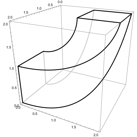
Figure 2: The three-dimensional domain

When using the Gauss-Seidel smoother, we again perform the multigrid method directly on the system matrix $\mathcal{B}_{h}$. When using the subspace corrected mass smoother, we perform the multigrid method on the auxiliary operator $\bar{\mathcal{B}}_{h}$, representing the reduced inner product $(\cdot,\cdot)_{\bar{\mathcal{B}}(\widehat{\Omega})}$ on the parameter domain. Again, we use that the matrices $\mathcal{B}_{h}$ and $\bar{\mathcal{B}}_{h}$ are spectrally equivalent with constants independent of $p$ and $h$, but which certainly depend on the geometry transformation. For the subspace corrected mass smoother, we choose $\sigma^{-1}:=0.015h^{4}$ for $d=2$ and $\sigma:=0.020h^{4}$ for $d=3$. Again, we choose $\tau=1$ in all cases.

$\ell$ $\backslash\;p$	3	4	5	6	7	8	9	10
Symmetric Gauss-Seidel
5	15	15	20	37	69	133	220	413
6	17	16	21	37	66	127	234	428
7	18	17	21	37	68	125	231	413
8	19	17	21	37	67	120	217	380
Subspace corrected mass smoother
5	162	161	152	150	142	134	130	127
6	196	200	200	194	180	179	178	171
7	215	220	225	222	219	210	198	198
8	226	232	243	233	227	221	217	210

Table 3: Iteration counts for 2D physical domain given in Figure 2

$\ell$ $\backslash\;p$	3	4	5	6	7
Symmetric Gauss-Seidel
3	14	32	93	262	763
4	23	35	94	246	634
5	36	37	88	226	516
6	51	45	90	220	OoM
Subspace corrected mass smoother
3	115	114	130	142	154
4	259	243	241	235	233
5	443	441	430	410	380
6	651	650	644	637	OoM

Table 4: Iteration counts for 3D physical domain given in Figure 2

Tables 3 and 4 show the number of iterations required to reduce the initial residual by a factor of $10^{-8}$. Again, we obtain very nice results for the Gauss Seidel smoother which – as for the case of trivial computational domains – deteriorate if $p$ is increased.

For the mass smoother, we have proven robustness in $p$ and $h$. Here, the results might look like the mass smoother is not robust in $h$. The reason is that a sufficiency small grid size $h$ is needed to capture the full effect of the geometry transformation. A similar observation can also be made for the Possion problem (cf. [16, Table 4]). The effects of the geometry transformation can be measured by the condition number of $\bar{\mathcal{B}}_{h}^{-1}\mathcal{B}_{h}$. For the Poisson problem, this condition number was estimated, e.g., in [31]. For the biharmonic problem, the condition number is typically the square of the condition number for the Poisson problem, which explains that the dependence on the geometry transformation is more severe for the biharmonic problem.

6.3 A hybrid smoother

The numerical experiments have shown that the Gauss-Seidel smoother captures the effects of the geometry transformation quite well and that it is superior to the mass smoother for nontrivial domains, unless $p$ is particularly high. The mass smoother is robust in $p$, but does not perform well for non-trivial geometries. So, it seems to be a good idea to set up a hybrid smoother which combines the strengths of both proposed smoothers.

We set up again a conjugate gradient solver, preconditioned with one multigrid V-cycle with $1$ pre and $1$ post smoothing step. Here, in order to represent the geometry well, the multigrid solver is set up on the original system matrix $\mathcal{B}_{h}$. The hybrid smoother consists of one forward Gauss-Seidel sweep, followed by one step of the subspace corrected mass smoother, finally followed by one backward Gauss-Seidel sweep. As always, the subspace corrected mass smoother – which requires a tensor-product matrix – is constructed based on the reduced matrix $\bar{\mathcal{B}}_{h}$ on the parameter domain. For the Gauss-Seidel sweeps, we choose $\tau=1$; and for the subspace corrected mass smoother, we choose $\tau=0.125$ and $\sigma^{-1}=0.015h^{4}$ for $d=2$ and $\tau=0.09$ and $\sigma^{-1}=0.015h^{4}$ for $d=3$.

Tables 5 and 6 show the iteration numbers for the hybrid smoother. We see that the iteration counts are quite robust both in the spline degree $p$ and in the grid level $\ell$. For small spline degrees, the iteration counts are comparable to the multigrid preconditioner with Gauss Seidel smoother. For high spline degrees, the hybrid smoother outperforms both other approaches, even if one considers that the overall costs for one step the hybrid smoother are comparable to the overall costs of two smoothing steps of one of the other smoothers.

$\ell$ $\backslash\;p$	3	4	5	6	7	8	9	10
Hybrid smoother
5	15	14	16	19	22	24	26	28
6	16	15	17	20	23	26	30	31
7	18	16	18	21	25	28	31	32
8	19	16	19	22	25	28	32	33

Table 5: Iteration counts for 2D physical domain given in Figure 2

$\ell$ $\backslash\;p$	3	4	5	6	7
Hybrid smoother
3	13	14	17	22	26
4	23	22	23	26	31
5	36	34	33	36	41
6	51	44	44	46	OoM

Table 6: Iteration counts for 3D physical domain given in Figure 2

References

• [1] T. J. R. Hughes, J. A. Cottrell, Y. Bazilevs, Isogeometric analysis: CAD, finite elements, NURBS, exact geometry and mesh refinement, Computer Methods in Applied Mechanics and Engineering 194 (39) (2005) 4135–4195.
• [2] L. Beirão da Veiga, A. Buffa, G. Sangalli, R. Vázquez, Mathematical analysis of variational isogeometric methods, Acta Numerica 23 (2014) 157–287.
• [3] P. G. Ciarlet, The finite element method for elliptic problems, SIAM, 2002.
• [4] V. Girault, P.-A. Raviart, Finite element methods for Navier-Stokes equations: theory and algorithms, Vol. 5, Springer Science & Business Media, 2012.
• [5] K.-A. Mardal, B. F. Nielsen, M. Nordaas, Robust preconditioners for PDE-constrained optimization with limited observations, BIT Numerical Mathematics (2015) 1–27.
• [6] J. Sogn, W. Zulehner, Schur complement preconditioners for multiple saddle point problems of block tridiagonal form with application to optimization problems, arXiv preprint 1708.09245.
• [7] J. Pestana, R. Muddle, M. Heil, F. Tisseur, M. Mihajlović, Efficient block preconditioning for a $C^{1}$ finite element discretization of the dirichlet biharmonic problem, SIAM Journal on Scientific Computing 38 (1) (2016) A325–A345.
• [8] S. Zhang, An optimal order multigrid method for biharmonic, ${C}^{1}$ finite element equations, Numerische Mathematik 56 (6) (1989) 613–624.
• [9] S. C. Brenner, An optimal-order nonconforming multigrid method for the biharmonic equation, SIAM Journal on Numerical Analysis 26 (5) (1989) 1124–1138.
• [10] S. Zhang, J. Xu, Optimal solvers for fourth-order pdes discretized on unstructured grids, SIAM Journal on Numerical Analysis 52 (1) (2014) 282–307.
• [11] M. R. Hanisch, Multigrid preconditioning for the biharmonic Dirichlet problem, SIAM Journal on Numerical Analysis 30 (1) (1993) 184–214.
• [12] A. Buffa, H. Harbrecht, A. Kunoth, G. Sangalli, BPX-preconditioning for isogeometric analysis, Computer Methods in Applied Mechanics and Engineering 265 (2013) 63–70.
• [13] K. Gahalaut, J. Kraus, S. Tomar, Multigrid methods for isogeometric discretization, Computer Methods in Applied Mechanics and Engineering 253 (2013) 413–425.
• [14] C. Hofreither, W. Zulehner, On full multigrid schemes for isogeometric analysis, in: T. Dickopf, M. Gander, L. Halpern, R. Krause, F. L. Pavarino (Eds.), Domain Decomposition Methods in Science and Engineering XXII, Springer International Publishing, 2016, pp. 267–274.
• [15] C. Hofreither, S. Takacs, W. Zulehner, A robust multigrid method for isogeometric analysis in two dimensions using boundary correction, Computer Methods in Applied Mechanics and Engineering 316 (2017) 22–42.
• [16] C. Hofreither, S. Takacs, Robust multigrid for isogeometric analysis based on stable splittings of spline spaces, SIAM Journal on Numerical Analysis 4 (55) (2017) 2004–2024.
• [17] S. Takacs, T. Takacs, Approximation error estimates and inverse inequalities for B-splines of maximum smoothness, Mathematical Models and Methods in Applied Sciences 26 (07) (2016) 1411–1445.
• [18] H. Blum, R. Rannacher, R. Leis, On the boundary value problem of the biharmonic operator on domains with angular corners, Mathematical Methods in the Applied Sciences 2 (4) (1980) 556–581.
• [19] P. Grisvard, Elliptic Problems in Nonsmooth Domains. Reprint of the 1985 hardback ed., Philadelphia, PA: Society for Industrial and Applied Mathematics (SIAM), 2011.
• [20] C. de Boor, A practical guide to splines, Springer, 1978.
• [21] J. Bergh, J. Löfström, Interpolation spaces: An introduction, Springer, 1976.
• [22] R. Adams, J. Fournier, Sobolev Spaces, Academic Press, 2008, 2nd ed.
• [23] S. Takacs, W. Zulehner, Convergence analysis of all-at-once multigrid methods for elliptic control problems under partial elliptic regularity, SIAM Journal on Numerical Analysis 51 (3) (2013) 1853–1874.
• [24] M. S. Floater, E. Sande, Optimal spline spaces for ${L}^{2}$ $n$-width problems with boundary conditions, arXiv preprint 1709.02710.
• [25] L. Schumaker, Spline functions: basic theory, Cambridge University Press, 2007.
• [26] S. Takacs, Robust approximation error estimates and multigrid solvers for isogeometric multi-patch discretizations, arXiv preprint 1709.05375.
• [27] W. Hackbusch, Multi-grid methods and applications, Vol. 4, Springer Science & Business Media, 2013.
• [28] C. Schwab, p- and hp- Finite Element Methods: Theory and Applications in Solid and Fluid Mechanics, Numerical Mathematics and Scientific Computation, Clarendon Press, 1998.
• [29] K. Scherer, A. Y. Shadrin, New Upper Bound for the B-Spline Basis Condition Number: II. A Proof of de Boor’s 2k-Conjecture, Journal of Approximation Theory 99 (2) (1999) 217 – 229.
• [30] A. Mantzaflaris, J. Sogn, S. Takacs, others (see website), G+Smo v0.8.1, http://gs.jku.at/gismo (2017).
• [31] G. Sangalli, M. Tani, Isogeometric preconditioners based on fast solvers for the Sylvester equation, SIAM Journal on Scientific Computing 38 (6) (2016) A3644–A3671.