Phase Stochastic Resonance in a forced nano-electromechanical oscillator

Abstract

Stochastic resonance is a general phenomenon usually observed in one-dimensional, amplitude modulated, bistable systems.We show experimentally the emergence of phase stochastic resonance in the bidimensional response of a forced nano-electromechanical membrane by evidencing the enhancement of a weak phase modulated signal thanks to the addition of phase noise. Based on a general forced Duffing oscillator model, we demonstrate experimentally and theoretically that phase noise acts multiplicatively inducing important physical consequences. These results may open interesting prospects for phase noise metrology or coherent signal transmission applications in nanomechanical oscillators. Moreover, our approach, due to its general character, may apply to various systems.

Stochastic resonance whereby a small signal gets amplified resonantly by application of external noise has been introduced originally in paleoclimatology Benzi ; GammaitoniRMP98 to explain the recurrence of ice ages and has then been observed in many other areas including neurobiology Douglass ; Bezrukov , electronics FauvePLA83 , mesoscopic physics Hibbs , photonics McNamara ; PhysRevE.61.157 , atomic physics PhysRevLett.85.1839 and more recently mechanics BadzeyNat05 ; PhysRevA.79.031804 ; VenstraNatCom13 ; MonifiNP16 . Implementation of stochastic resonances involves generally three ingredients : (i) the existence of metastable states separated by an activation energy, as in excitable or bistable nonlinear systems, (ii) a coherent excitation, whose amplitude is however too weak to induce deterministic hopping between the states, and (iii) stochastic processes inducing random jumps over the potential barrier. In the classical picture of a bistable system, this corresponds to the motion of a fictive particle in a double-well potential periodically modulated in amplitude by the signal and subjected to noise PhysRevLett.62.349 . When an optimal level of noise is reached, the system’s response power spectrum displays a peak in the signal to noise ratio, unveiling the stochastic resonance phenomenon. The resonance occurs as a ’bona-fide’ resonance in a frequency band around a signal frequency approximately given by the time-matching condition GammaitoniPRL95 ; BarbayPRL00 , i.e. when the potential modulation period is twice the mean residence time of the noise-driven particle. Experimental works on stochastic resonance are almost exclusively using amplitude modulation going along with additive amplitude noise or multiplicative amplitude noise PhysRevE.49.4878 ; PhysRevE.61.940 ; WuJoMO07 ; WuPRA09 ; QiaoPRE16 . In this case, it corresponds to a pure one dimensional effect. Few studies take advantage of a bidimensional phase space by e.g. using phase modulation and/or phase noise (i.e. phase random fluctuations of input signal) doi:10.1021/nl9004546 ; Guerra . Most of them use amplitude noise to demonstrate amplitude stochastic resonance, or introduce noise in the form of the response of a stochastic oscillator Schimansky-Geier1990 . However in the latter scheme, neither the noise nor the modulation are controlled, thus preventing to unveil the specific roles of phase modulation and phase noise in stochastic resonance.

In this Letter, stochastic resonance is implemented in a nonlinear nanomechanical oscillator forced close to its resonant frequency. It enables, in a bidimensionnal phase space, the implementation of phase stochastic resonance observed simultaneously both on the phase and amplitude response of the oscillator. It is here demonstrated by achieving the stochastic enhancement of a phase modulated signal by phase noise observed on the bidimensional response of the oscillator. This opens new avenues for stochastic resonance in bidimensional systems by allowing for instance stochastic amplification of mixed phase-amplitude modulated signals by complex value noise. We highlight that the system’s response can be projected on any variable in phase space and that the amplification depends on the chosen basis. Finally, we derive a stochastic nonlinear amplitude equation for the forced stochastic Duffing oscillator, which describes qualitatively well our system, and show that phase noise acts multiplicatively inducing important physical consequences.

The forced nanomechanical oscillator consists of a suspended InP photonic crystal membrane which acts as a mirror in one arm of an interferometer fed with an He-Ne laser. The membrane is activated by underneath integrated interdigitated electrodes driven by an AC-bias voltage $V\left(t\right)$ (see Fig. 1). This voltage induces an electrostatic force on the oscillator which drives its out-of-plane motion as described in Chowdhury . The oscillator is placed in a vacuum chamber with a pressure of about $10^{-4}$ mbar at room temperature. The phase $\Phi$ and the amplitude modulus $R$ of the oscillator’s motion are retrieved by use of a balance homodyne detection. From the recorded time traces of $\Phi$ and $R$, we can reconstruct the polar plots with the two quadratures $X=R\cos\left(\Phi\right)$ and $Y=R\sin\left(\Phi\right)$.

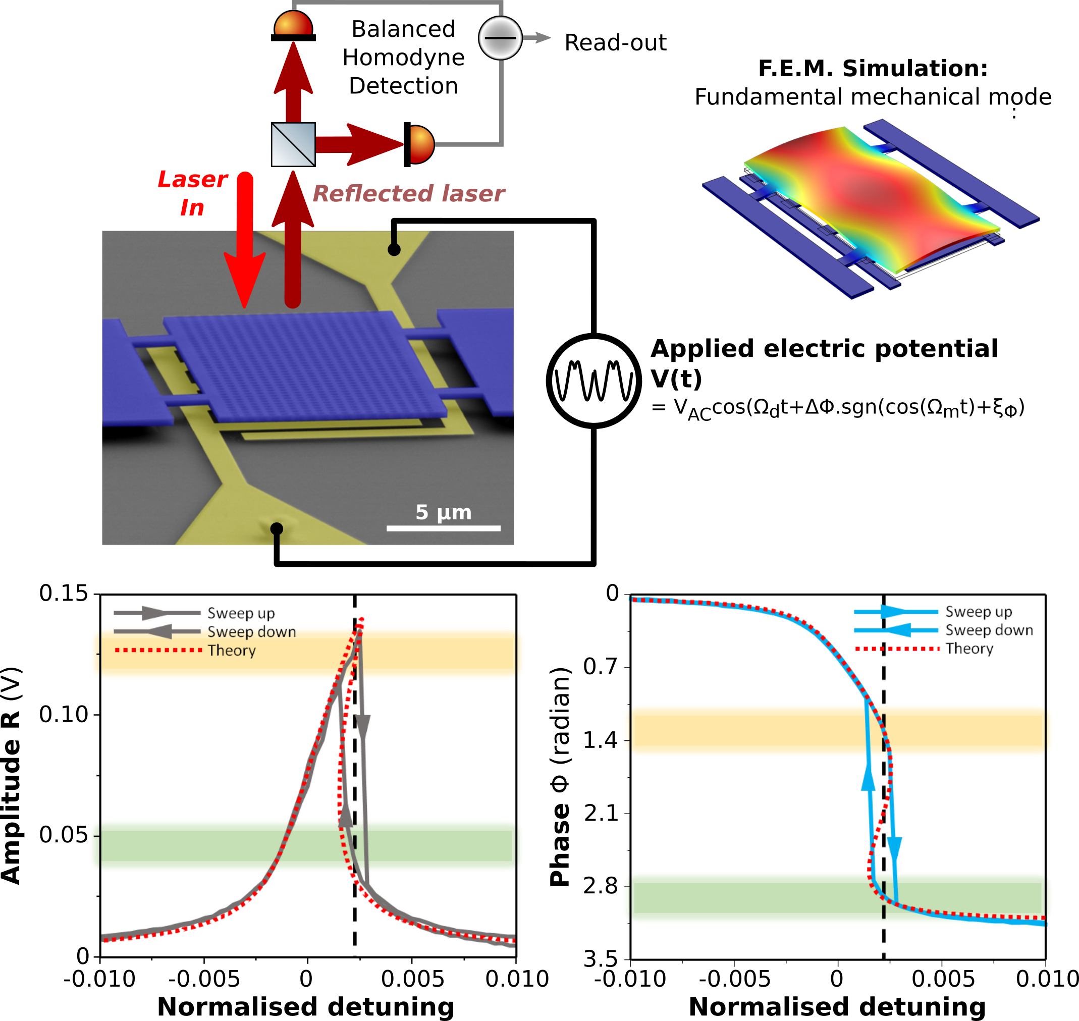
Figure 1: (Top left) A scanning electron microscopic view of the device shows the membrane (thickness of 260 nm and a 10$\times$20$\mu$m² surface) forming the mechanical oscillator (purple) and the interdigitated electrodes (yellow) underneath, at a distance of about 400 nm. (Top right) Finite Element Model (F.E.M.) simulation of the fundamental mechanical mode under study with enhanced out-of-plane displacement for clarity. (Bottom left) Amplitude $R$ and (bottom right) phase $\Phi$ spectra of the driven oscillator response in a frequency sweep-up and sweep-down experiment with $V_{AC}=9\,V$, $\Delta\phi=0$ and $\xi_{RMS}=0$; the theoretical response is displayed in red dashed lines in both spectra. The driving frequency $\nicefrac{{\Omega_{d}}}{{2\pi}}=2.824\,MHz$ (dashed lines) lies close to the linear fundamental mechanical resonance at ${\color[rgb]{1,0,0}{\color[rgb]{0,0,0}\nicefrac{{\Omega_{0}}}{{2\pi}}=}}2.822\,MHz$ (i.e. zero normalised detuning). Normalized detuning is defined as $\left(\Omega_{d}-\Omega_{0}\right)/\Omega_{0}$.

The applied voltage, and therefore the applied electrostatic force, is in the form of makles:tel-01290469 :

$$V\left(t\right)=V_{AC}\cos\left[\Omega_{d}t+\Delta\phi\ \mathrm{sgn}\left(\cos\left(\Omega_{m}t\right)\right){\color[rgb]{0,0,0}{\color[rgb]{1,0,0}{\color[rgb]{0,0,0}+\xi\left(t\right)}}}\right].$$ (1)

Here $V_{AC}$ is the amplitude of the applied voltage, while $\Omega_{d}$ denotes the resonant driving frequency. A phase modulation is added; it displays a square waveform described by the sign function $sgn$, at frequency $\Omega_{m}$ and a phase deviation of $\Delta\phi$. Gaussian phase noise $\xi(t)$ of zero-mean and standard deviation $\xi_{RMS}$ (bandwidth $B_{\phi}=10\,kHz$ such that $\Omega_{m}\ll B_{\phi}$) is also applied on the nonlinear dynamic system. Under quasi-resonant forcing of the mechanical fundamental mode, a hysteresis behavior becomes prominent for $V_{AC}>5\,V$ and two stable fixed points co-exist in the bidimensional phase space of the oscillator (Fig. 1-bottom left and right). In the following, $V_{AC}$ is set to $9\,V$ in order to be deeply in the bistable regime; the driving frequency is set inside the hysteresis region at $\nicefrac{{\Omega_{d}}}{{2\pi}}=2.824\,MHz$ in order to get equal probability of residence in each state (See Supplementary Information) and the system is systematically initially prepared in its upper state.

In the bistability regime, jumps between the two stable states can be induced by applying a slow modulation ($\Omega_{m}\ll\Omega_{d}$) with a sufficiently high phase deviation, phase noise strength or both. These jumps are investigated by tracing the amplitude and phase evolution of the fundamental mode with time and are also pictured in the X-Y phase plane. In the case of pure phase modulation, the system can transit or not from one state to the other depending on the values of $\Omega_{m}$ and $\Delta\phi$. Beyond the cut-off frequency $\nicefrac{{\Omega_{m,c}}}{{2\pi}}=1\,kHz$, which is directly linked to the oscillator’s line width of $0.9\,kHz$ Guerra , the output signal is not synchronized with the input signal, in amplitude or phase. For $\nicefrac{{\Omega_{m}}}{{2\pi}}=500\,Hz$, every jumps in the input signal translate into a jump in the output signal for $\Delta\phi>1.83\,rad$ (see Supplementary Information). Similarly, in the case of pure noise-induced switching, the system starts to transit between the two 2D states, in amplitude and phase as noise strength increases. The occupancy between these two states becomes equiprobable for values of $\xi_{RMS}$ close to $0.52\,rad$ in our device. Such noise-induced transitions can also be quantified by the Kramers rate $T_{K}=\nicefrac{{1}}{{\tau_{K}}}$ which is the inverse of the average time required to cross over the barrier KRAMERS1940284 and reaches a value close to $100\,Hz$ (see Supplementary Information). Contrary to amplitude noise which amounts to additive noise, phase noise acts here as a multiplicative noise. This feature is revealed through the non-constant dependence of the phase difference $\Delta\theta$ between the two equilibria for increasing noise strengths (see Fig. 2) and is highlighted by the fourth term in the right hand side of Eq. 4. At weak phase noise ($\xi_{RMS}<0.4\,rad$), uncertainties on the phase difference are large because the probability of residence in the lower state is weak ($<5\,\%$) and thus this state gets difficult to observe. Conversely, at strong phase noise ($\xi_{RMS}>0.6\,rad$), the probability of residence of the upper state reduces, and this state is hardly observable.

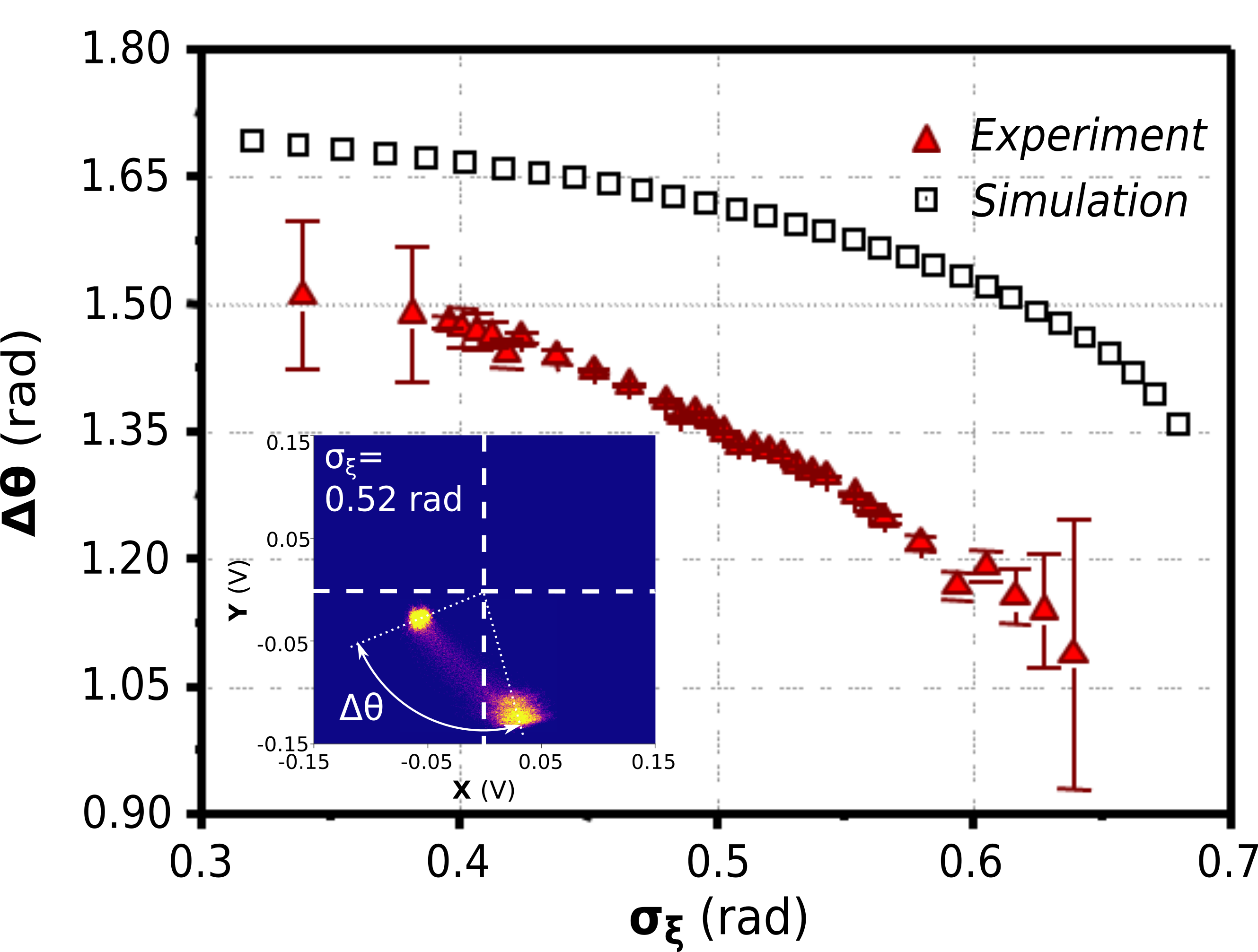
Figure 2: Simulated (open squares) and experimental (red triangles) polar angle difference between the two stable states for increasing noise strengths. Inset: Experimental polar plots with experimental values of $\xi_{RMS}=0.52\,rad$ and $\nicefrac{{\Omega_{d}}}{{2\pi}}=2.824\,MHz$.

The stochastic synchronization between the external noise and the weak coherent signal that occurs in stochastic resonance, takes place when the average waiting time between two noise-induced interwell transitions ($T_{K}$) is comparable to half the period of the periodic signal ($T_{\varOmega}=\nicefrac{{2\pi}}{{\Omega_{m}}}$). In order to match this time-scale condition, modulation frequency $\Omega_{m}$ in phase is set at $50\,Hz$. The deviation $\Delta\phi$ is also set to $0.09\,rad$ ($\ll 1.56\,rad$, the hysteresis width (Fig. 1)), a far too weak value to let the system switch periodically from one state to the other (see Fig. 3 upper line). When increasing the noise strength, occasional transitions occur, weakly locked to the modulation signal. For $\xi_{RMS}=0.49\,rad$, the transitions get stochastically synchronized with the modulation (see Fig. 3). Further increasing the noise distorts the hysteresis cycle and the system drops to its lower state.

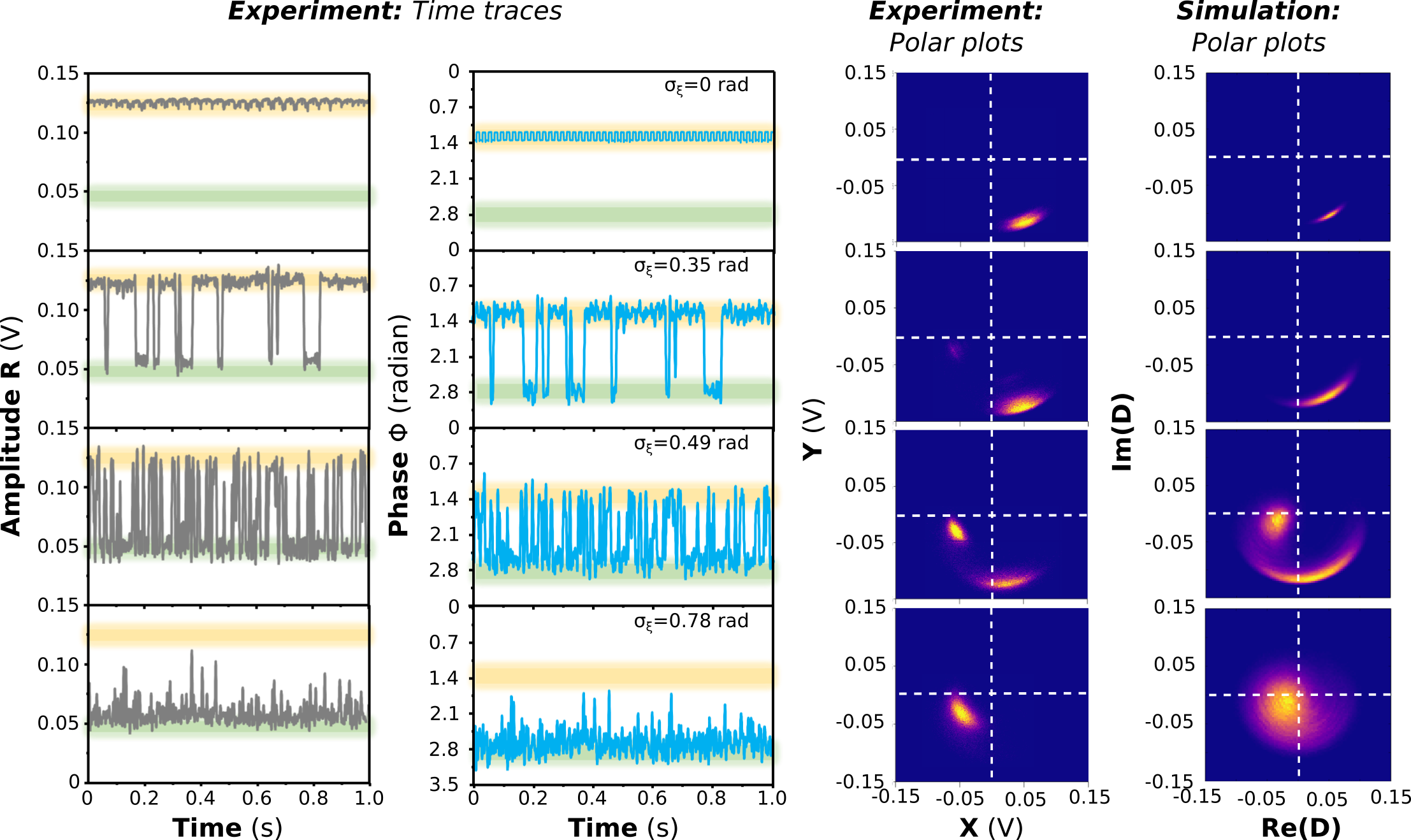
Figure 3: The response of the system, now driven by a force combining a weak phase modulation and an increasing phase noise is shown. (From left to right) Experimental time traces recorded on a timescale of $300\,s$ of the amplitude $R$ and phase $\Phi$ of the fundamental mode for increasing noise strengths, with associated experimental and theoretical polar plots. (From upper to lower lines) Evolution of these four panels for increasing standard deviation $\xi_{RMS}$.

Quantification of achieved amplification relies on a Discrete Fourier Transform (DFT) of the time traces. The spectral power amplification is then given by the ratio between the strength of the peak in the DFT at $\Omega_{m}$ for a given noise intensity and its strength without added noise. For both variables, $R$ and $\Phi$, evolution of the spectral amplification is observed as a function of the phase noise strength and are plotted on Fig. 4-a and b. It presents a bell-shaped maximum which reaches, for the amplitude variable, a value up to ${\color[rgb]{0,0,0}{\color[rgb]{0,0,0}6.3}}$ and peaks at $\xi_{RMS}=0.44\,rad$ (see Fig. 4-a). This noise strength is close to the one at which the system has a Kramer’s rate of about $100\,Hz$ with only noise applied. Under the same conditions, amplification of the phase variable is also shown in Fig. 4-b. It reaches experimentally a value up to 3 for the same phase noise strength. A double peak is clearly visible in the numerical spectral amplification of the phase. The first peak is indeed attributed to the synchronized hopping between the two metastable states, whereas the other peak is due to an internal state resonance PhysRevE.62.299 . For higher noise strength, the noise-induced effective detuning makes a longer residence time in the lower state, and the Kramers rates are not balanced anymore.

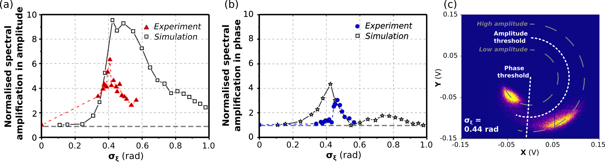
Figure 4: (a) Experimental (red triangles) and theoretical (open black squares) spectral amplification in amplitude $R$ as a function of phase noise strength. (b) Experimental (blue circles) and theoretical (open black stars) spectral amplification in phase $\Phi$ as a function of phase noise strength. Theoretical curves have been obtained by use of Eq.(4). (c) Experimental polar plot for $\xi_{RMS}=0.44\,rad$ (maximum amplification), highlighting the shape of the two stable points as well as the directions imprinted by the modulation on the input phase or amplitude. The two dashed grey lines are guide for the eyes indicating the two distinct amplitude states and the dotted white line highlights the threshold.

To gain more insight into the observed dynamics, we compare our results to theoretical and numerical predictions of a stochastic amplitude equation. Fits of the experimental results are obtained by modeling the nano-electromechanical oscillator by a simple forced stochastic Duffing oscillator Duffing18 whose dynamics can be described, in the limit of small injection and dissipation of energy, by:

$$\ddot{x}=-x-\epsilon\mu\dot{x}-\alpha x^{3}+\\ \epsilon^{3/2}F\cos((1+\epsilon\sigma)t+\epsilon\phi_{m}(t)+\epsilon\sqrt{\eta_{0}}\Delta W_{\phi})$$ (2)

where $x(t)$ accounts for the displacement of the membrane and $\epsilon$ is a small control parameter ($\epsilon\ll 1$). This parameter is introduced to properly balance the scaling between the dissipation and injection of energy in the system, and also control the frequency detuning. The natural frequency has been rescaled to one ($\omega_{0}=1$), $\mu\ll 1$ is the damping coefficient that accounts for dissipation of energy, $\alpha$ accounts for the nonlinear stiffness of the spring, which is positive (negative) for soft (hard) spring Bogoliubov61 and $F$ the strength of the driving. The near-resonant drive has an angular frequency of $\omega_{d}=1+\sigma$, where $\sigma\ll 1$ stands for the detuning between the drive and the natural resonant frequency. The system is also subject to a slow phase modulation $\phi_{m}(t)$ ($\dot{\phi}_{m}\ll\omega_{0}\phi_{m}$) and to a phase noise term in the form of a Wiener process $\Delta W_{\phi}$ with Gaussian noise strength $\eta_{0}$. In the conservative limit and for small displacements, the system exhibits harmonic motion with a small arbitrary amplitude $D$ such that $x(t)=Re[De^{it}]$. When considering the nonlinear terms, dissipation and forcing, the displacement of the membrane response can be approximated by Bogoliubov61 ; Kevorkian96 :

$$x(t) = \epsilon^{3/2}D(T=\epsilon t)e^{i[t+\epsilon(\sigma t+\phi_{m}(t)+\sqrt{\eta_{0}}\Delta W_{\phi})]}$$

$$+\frac{\alpha\epsilon^{9/2}}{8}D^{3}e^{i3[t+\epsilon(\sigma t+\phi_{m}(t)+\sqrt{\eta_{0}}\Delta W_{\phi})]}+c.c.+o(\epsilon^{5})$$ (3)

where the envelope of the oscillations $D$ is promoted to a temporal variable Bogoliubov61 ; Kevorkian96 ; NewellARoFM93 , $T$ accounts for the slow temporal scale ($\dot{D}\simeq\epsilon D$ and $\ddot{D}\simeq\epsilon^{2}D$), and the symbol $c.c.$ stands for complex conjugate. Introducing the above ansatz in Eq. (2) to order $\epsilon^{3/2}$ and using the rules of calculus in stochastic normal form theory ClercPRE06 one finds the stochastic nonlinear amplitude equation:

$$\frac{dD}{dT}=-(\frac{\mu}{2}+i(\sigma+\frac{d\phi_{m}}{dT}+\sqrt{\eta_{0}}\xi))D+\frac{3i\alpha}{8}|D|^{2}D-\frac{iF}{2}$$ (4)

where $\xi=d\Delta W_{\phi}/dT$ is a zero-mean and delta-correlated white Gaussian noise term. Note that $\phi_{m}$ is a slow phase modulation, that is, $d\phi_{m}/dt=\epsilon d\phi_{m}/dT$. To derive the above model, we have considered ansatz (3) as a change of variable. Here, the Stratonovich prescription for noise has been adopted. Namely, the stochastic term can induce a non-zero drift, $\left\langle\xi\left(T\right)D\left(T\right)\right\rangle\neq 0$. Note that even though Eq.(2) would give rise to additive noise with time-dependent coefficients in a Fokker-Planck equation, the reduced equation (Eq.(4)) for the response amplitude of the oscillations satisfies a stochastic differential equation with multiplicative noise as a result of the stochastic normal-form derivation ClercPRE06 .

Stochastic numerical simulations of Eq.(4) are performed with the help of the XMDS2 package DennisCPC13 . We use the semi-implicit numerical scheme which converges to the Stratonovich integral. The time step is kept fixed in the simulation and is chosen to be $dT=0.1$. The slow phase modulation is sinusoidal with an amplitude $\Delta\phi=5\times 10^{-5}$ and an angular frequency $\Omega_{m}=2\pi/2\times 10^{5}$. The detuning is $\sigma=1.77\times 10^{-3}$. The model reproduces well the bistable response in amplitude and phase of our nano-electromechanical oscillator (see Fig. 1 bottom), as well as the temporal evolution of the response in amplitude or phase, in the case of pure phase modulation, pure phase noise (see Supplementary Information) and stochastic resonance (see Fig. 3 and 4). Moreover, multiplicative noise shall translate into a shift of the operating point in the hysteresis and thus into an effective detuning in Eq. (4) which reduces to $\sigma_{eff}=\sigma+\eta_{0}/2$. Physically, this translates in a drift of the operating point for increased noise strengths, a signature of the multiplicative nature of the added noise, as observed in our experiment (see Fig. 2). The measured $\Delta\theta$ is slightly smaller in the experiment compared to theory presumably because of extra low-frequency noise sources which are not taken into account in the model.

Stochastic resonance amplification of the modulated signal is here limited by the relative orientation of the modulation and of the minimal energy path between the two basins of attraction, which is almost in a direct straight line (see Fig. 4-c). In the same frame, the added phase modulation shakes the upper state preferentially in the azimuthal direction. These two orientations being not parallel, higher amplification value can not be achieved in this configuration. This reveals the importance of the modulation format of the signal: optimal stochastic resonance would certainly require a mixed amplitude-phase format to follow the minimal energy path in the nanomechanical oscillator phase space. The distribution of the two states in the phase plane gets also distorted: The system switches between a symmetric branch (with a quasi-circular state in the phase portrait) to an asymmetric branch (with an elongated state in the polar plot). Such distortion is reminiscent to thermal noise squeezing observed e.g. in parametrically-driven oscillators RugarPRL91 ; BriantEPJD03 ; SzorkovszkyPRL13 ; PontinPRL16 .

In conclusion, we have demonstrated phase stochastic resonance with phase noise in a bidimensional nonlinear oscillator consisting of a nano-electromechanical device. The applied phase noise reveals to act as a multiplicative noise on the system which introduces an effective detuning that plays a crucial role in the residence probability asymmetry. The derived stochastic amplitude equation (4) is a universal model that describes the evolution of the envelope of the oscillations near a nonlinear resonance and subjected simultaneously to phase noise and to a phase modulation. That is, it applies to any nonlinear oscillator with such forcing provided one makes use of a suitable nonlinear and periodic change of variables in the initial equations that describe the system. Our model applies to e.g. dispersive optical bistability that plays an important role in nonlinear optical science TalknerPRA84 and can thus shed a new light on coherent processes involving phase fluctuations in these systems CasteelsPRA17 . Such stochastic resonance obtained by the assistance of phase noise may also enable various noise-aided applications, including signal transmission JungPRA91 ; PhysRevLett.85.3369 in particular involving novel coherent schemes such as Phase Key Shifting protocol, or metrology with improved detection in noise-floor limited systems PhysRevE.61.940 ; PhysRevLett.102.080601 ; 10.1371/journal.pone.0109534 .

References

- (1) , Benzi, R. and Sutera, A. and Vulpiani, A. J. Phys. A: Math. Gen 14, 453-457, 1981
- (2) ,Alfonsi, L. and Gammaitoni, L. and Santucci, S. and Bulsara, A. R., Phys. Rev. E 62, 299 (2000)
- (3) , Badzey, R. L. and Mohanty, P., Nature 437, 995–998 (2005)
- (4) , Barbay, Sylvain and Giacomelli, Giovanni and Marin, Francesco, Phys. Rev. E 61, 157, (2000)
- (5) , Barbay, Sylvain and Giacomelli, Giovanni and Marin, Francesco, Phys. Rev. Lett. 85, 4652 (2000)
- (6) , Bezrukov, Sergey M. and Vodyanoy, Igor, Nature 378, 362-364 (1995)
- (7) , Bogoliubov, N. N. and Mitropolski, Y. A., Asymptotic Methods in the Theory of Non-Linear Oscillations, New York: Gordon and Breach (1961)
- (8) , T. Briant and P. F. Cohadon and M. Pinard and A. Heidmann, Eur. Phys. J. D 22, 131, (2003)
- (9) , Casteels, W. and Fazio, R. and Ciuti, C., Phys. Rev. A 95, 012128 (2017)
- (10) , Chapeau-Blondeau, Francois, Phys. Rev. E 61, 940 (2000)
- (11) , A. Chowdhury and I. Yeo, V. Tsvirkun and F. Raineri and G. Beaudoin and I. Sagnes and R. Raj and I. Robert-Philip and R. Braive, Appl. Phys. Lett. 108, 163102 (2016)
- (12) , Clerc, M. G. and Falcón, C. and Tirapegui, E., Phys. Rev. E 74, 011303 (2006)
- (13) , Cottone, F. and Vocca, H. and Gammaitoni, L., Phys. Rev. Lett. 102, 080601 (2009)
- (14) , Graham R. Dennis and Joseph J. Hope and Mattias T. Johnsson, Computer Physics Communications 184, 201, (2013)
- (15) , Diego, Guerra and Matthias, Imboden and Pritiraj, Mohanty, Appl. Phys. Lett. 93, 033515, (2008)
- (16) , Douglass, John K. and Wilkens, Lon and Pantazelou, Eleni and Moss, Frank, Nature 365, 337 (1993)
- (17) , G. Duffing, F. Vieweg u. Sohn, Braunschweig (1918)
- (18) , S. Fauve and F. Heslot, Physics Letters A 97, 5 (1983)
- (19) , Gammaitoni, Luca and Hänggi, Peter and Jung, Peter and Marchesoni, Fabio, Rev. Mod. Phys. 70, 223 (1998)
- (20) , Gammaitoni, L. and Marchesoni, F. and Menichella-Saetta, E. and Santucci, S., Phys. Rev. E 49, 4878 (1994)
- (21) , Gammaitoni, L. and Marchesoni, F. and Menichella-Saetta, E. and Santucci, S., Phys. Rev. Lett. 62, 349 (1989)
- (22) , Gammaitoni, L. and Marchesoni, F. and Santucci, S., Phys. Rev. Lett. 74, 1052 (1995)
- (23) , Guerra, Diego N. and Dunn, Tyler and Mohanty, Pritiraj, Nano Letters 9, 3096 (2009)
- (24) , Herrera-May, AgustÃn L. AND Tapia, Jesus A. AND DomÃnguez-Nicolás, Saúl M. AND Juarez-Aguirre, Raul AND Gutierrez-D, Edmundo A. AND Flores, Amira AND Figueras, Eduard AND Manjarrez, Elias, PLOS ONE 9, 1 (2014)
- (25) , A. D. Hibbs and A. L. Singsaas and E. W. Jacobs and A. R. Bulsara and J. J. Bekkedahl and F. Moss, J. Appl. Phys. 77, 2582 (1995)
- (26) , Inchiosa, M. E. and Robinson, J. W. C. and Bulsara, A. R., Phys. Rev. Lett. 85, 3369 (2000)
- (27) , Jung, Peter and Hänggi, Peter, Phys. Rev. A 44, 8032 (1991)
- (28) , J.K. Kevorkian and J.D. Cole, Multiple Scale and Singular Perturbation Methods, Springer-Verlag, New York (1996)
- (29) , H.A. Kramers, Physica 7, 284, (1940)
- (30) , Makles, Kevin, Optomechanic’s photonic crystal nano-membranes, Thesis Université Pierre et Marie Curie - Paris VI (2015)
- (31) , Masoller, C., Phys. Rev. Lett. 88, 034102 (2002)
- (32) , McNamara,Bruce and Wiesenfeld, Kurt and Roy, Rajarshi, Phys. Rev. Lett. 60, 2626 (1988)
- (33) , Monifi, Faraz and Zhang, Jing and Özdemir, Şahin Kaya and Peng, Bo and Liu, Yu-xi and Bo, Fang and Nori, Franco and Yang, Lan, Nat Photon 10, 399 (2016)
- (34) , Mueller, F. and Heugel, S. and Wang, L. J., Phys. Rev. A 79, 031804 (2009)
- (35) , A. C. Newell and T. Passot and J. Lega, Annual Review of Fluid Mechanics 25, 399 (1993)
- (36) , Pontin, A. and Bonaldi, M. and Borrielli, A. and Marconi, L. and Marino, F. and Pandraud, G. and Prodi, G. A. and Sarro, P. M. and Serra, E. and Marin, F., Phys. Rev. Lett.116, 103601 (2016)
- (37) , Qiao, Zijian and Lei, Yaguo and Lin, Jing and Niu, Shantao, Phys. Rev. E 94, 052214 (2016)
- (38) , Rugar, D. and Grütter, P., Phys. Rev. Lett. 67, 699 (1991)
- (39) , Schimansky-Geier, L. and Zülicke, Ch., Zeitschrift für Physik B Condensed Matter 79, 451 (1990)
- (40) , Szorkovszky, A. and Brawley, G. A. and Doherty, A. C. and Bowen, W. P., Phys. Rev. Lett. 110, 184301 (2013)
- (41) , Talkner, Peter and Hänggi, Peter, Phys. Rev. A 29, 768 (1984)
- (42) , Venstra, Warner J. and Westra, Hidde J. R. and van der Zant, Herre S. J., Nat Commun 4 (2013)
- (43) , Wilkowski, David and Ringot, Jean and Hennequin, Daniel and Garreau, Jean Claude, Phys. Rev. Lett. 85, 1839 (2000)
- (44) , Haibin Wu and Amitabh Joshi and Min Xiao, Journal of Modern Optics 54, 2241 (2007)
- (45) , Wu, Haibin and Singh, Surendra and Xiao, Min, Phys. Rev. A 79, 023835 (2009)