A Modified Sigma-Pi-Sigma Neural Network with Adaptive Choice of Multinomials
ABSTRACT
Sigma-Pi-Sigma neural networks (SPSNNs) as a kind of high-order neural networks can provide more powerful mapping capability than the traditional feedforward neural networks (Sigma-Sigma neural networks). In the existing literature, in order to reduce the number of the Pi nodes in the Pi layer, a special multinomial is used in SPSNNs. Each monomial in is linear with respect to each particular variable when the other variables are taken as constants. Therefore, the monomials like or with are not included. This choice may be somehow intuitive, but is not necessarily the best. We propose in this paper a modified Sigma-Pi-Sigma neural network (MSPSNN) with an adaptive approach to find a better multinomial for a given problem. To elaborate, we start from a complete multinomial with a given order. Then we employ a regularization technique in the learning process for the given problem to reduce the number of monomials used in the multinomial, and end up with a new SPSNN involving the same number of monomials (= the number of nodes in the Pi-layer) as in . Numerical experiments on some benchmark problems show that our MSPSNN behaves better than the traditional SPSNN with .
1 Introduction
Sigma-Pi-Sigma neural networks (SPSNNs) [1,4,7,8] as a kind of high-order neural networks can provide more powerful mapping capability [2-3,5,6] than the traditional feedforward neural networks (Sigma-Sigma neural networks). In an SPSNN, a Pi layer (denoted by layer hereafter) is inserted in between the two Sigma layers. Each Pi node ( node) in the layer corresponds to a monomial, of which the variables are the outputs of the Sigma nodes ( nodes) of the first Sigma layer ( layer). Each node in the second Sigma layer ( layer) implements a linear combination of the outputs of the layer, and therefore represents a multinomial expansion of the output of the layer. Then, the multinomial expansion is processed by an activation function in the layer to give the final output of the network.
At the beginning of the development of SPSNN, researchers have realized that it is not a good idea to include all the possible monomials in the layer, i.e., to get a complete multinomial expansion of the layer, since it results in too many nodes in the layer. In the existing literature, in order to reduce the number of nodes, a special multinomial (called multi-linear multinomial) is used in SPSNNs. The monomials in are linear with respect to each particular variable when taking the other variables as constants. Therefore, the monomials such as or with are not included in . An intuitive idea behind this strategy may be the following: A node should receive at most one signal, rather than two or more signals, from each node.
But from general numerical approximation point of view, each monomial plays equally important role for approximating nonlinear mappings by using multinomial. Thus, the special multi-linear multinomial may not be the best choice for the SPSNN to approximate a particular nonlinear mapping. To this end, we propose an adaptive approach to find a better multinomial for a given problem. To elaborate, we start from a complete multinomial with a given order. Then we employ a regularization technique in the learning process for the given problem to reduce the number of monomials used in the multinomial, and end up with a modified SPSNN (MSPSNN) involving the same number of monomials (= the number of nodes in the layer) as in . In particular, a smoothing regularization term [10,15] is used as an example in our method, which has been successfully applied for various kinds of neural network regularization.
We divide the learning process of MSPSNN into two phases. The first phase is a structural optimization phase. Here, we insert a regularization term into the usual error function for SPSNN involving a complete set of multinomials, and perform a usual gradient learning process. In the end, we delete the nodes with smaller - weights, and obtain a network with the same number of nodes as in .
The second learning phase is a refinement phase. We re-start a gradient learning process for the network obtained from the first learning phase, and use the weights that survived the first phase as the initial weights. The aim of the refinement phase is to make up for the loss caused by the deleted nodes in the first learning phase.
Numerical experiments are performed on some benchmark problems including two approximation problems and two classification problems. It is shown that our new MSPSNN behaves better than the traditional SPSNN with .
The rest of the paper is arranged as follows. The proposed MSPSNN with smoothing regularization term is described in Section 2. In Section 3, Supporting numerical simulations are presented. Some conclusions are given in Section 4.
2 MSPSNN method with smoothing regularization
2.1 Sigma-Pi-Sigma neural network
An SPSNN is composed of an input layer, two hidden layers of summation node layer ( layer) and product node layer ( layer), and an output layer ( layer). The numbers of nodes of these layers are and 1, respectively.
Denote by the input vector, where the M components are the “real” input, while is an extra artificial input, fixed to -1. The output vector of layer with respect to can be written as
| (1) |
where is a given nonlinear activation function, is the weight vector connecting the -th summation node of layer and the input layer, and denotes the inner product of and . Here we remark that the component usually represents the bias of the -th summation node of layer.
In layer, Each node connects with certain nodes of layer, receives signals from these nodes, and outputs a particular monomial such as
| (2) |
Denote by the index set of all the nodes in layer that are connected to the -th node. For instance, let us assume that the above three examples in (2) correspond to the first, third and fifth nodes of layer, respectively. Then, we have
| (3) |
The output vector of layer is computed by
| (4) |
Here we make a convention that , when , i.e., when the -th node is not connected to any node of layer. The choice of ’s is our main concern in this paper.
Before we concentrate our attention on the choice of ’s, let us describe the output of layer. The output of the single node of layer, i.e., the final output of the network, is
| (5) |
where is another given activation function, and is the weight vector connecting layer and layer. When the network is used for approximation problems, we usually set . On the other hand, when the network is used for classification problems, is usually chosen to be a Sigmoid function. In both the cases, we can see from (1), (4) and (5) that the input to layer is actually a multinomial expansion of the output values of layer, where the components of correspond to the monomials, and the components of are the coefficients, involved in the multinomial expansion. As comparison, we recall that for the usual feedforward neural networks, the input to the layer is a linear combination of the output values of layer.
Now we discuss the choice of ’s in detail and explain the main idea of the paper. For convenience and clarity, we take the third order multinomial of three variables as an example in this introduction section. Therefore, we have , i.e., layer has three nodes.
We consider three choices of ’s, resulting in three different multinomial expansions: the complete mutinomial, the partially linear multinomial (the traditional approach), and the adaptive multinomial (our proposed approach).
The choice of the complete mutinomial means that the input to layer is a complete multinomial as follows:
| (6) |
We see that there are twenty monomials in the multinomial expansion, corresponding to twenty nodes in layer. More generally, when layer has nodes, the number of the monomials is , which grows very rapidly when increases. Therefore, the complete multinomial approach is not a good choice in practice.
The traditional choice in the existing literature is the partially linear multinomial approach: A partially linear multinomial is linear with respect to each particular variable , with the other variables taken as constants. For instance, the partially linear multinomial corresponds to (2.1) is
| (7) |
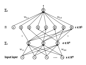
We see that there are only eight monomials in (7), i.e., only eight nodes left in layer. Generally, when layer has nodes, the number of the monomials is . Table 1 shows the comparison of and with different . It can be seen that the difference becomes bigger when increases.
| 3 | 4 | 5 | 6 | 7 | 8 | 9 | 10 | |
| 20 | 35 | 56 | 84 | 120 | 165 | 220 | 286 | |
| 8 | 15 | 26 | 42 | 64 | 93 | 130 | 176 | |
| Difference | 12 | 20 | 30 | 42 | 56 | 72 | 90 | 110 |
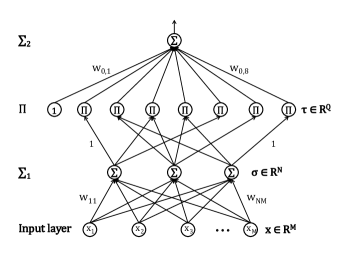
The network structure corresponding to (7) is shown in Fig. 3. The corresponding ’s are as follows:
| (8) |
We observe that in (2.1) and (7), the first product node, corresponding to the bias , does not connect with any node in the layer, so . We also notice that there are no repeated indexes in each in (8).
Our proposed choice is as follows: We start from a complete multinomial with a given order. Then we employ a regularization technique in the learning process to reduce the number of monomials used in the multinomial, and end up with a new SPSNN involving the same number of monomials as in the traditional choice. For instance, in the Example 1 given in Section 4.1 below, a new SPSNN is obtained with the following multimonial:
| (9) |
And correspondingly,
| (10) | |||
We notice that now there are some repeated indexes in six ’s.
2.2 Error function with regularization
Let the training samples be , where is the -th input sample and is its corresponding ideal output. Let be the network output for the input . The aim of the training process is to build up a network such that the errors are as small as possible. A conventional square error function with no regularization term is as follows:
| (11) |
where ,
| (12) |
Let us derive the gradient of the error function . Notice
| (13) |
and
| (14) |
Then, the partial derivative of with respect to is
| (15) |
Moreover, for , and , we have
| (16) |
According to (4) and (16), for any , we have
| (17) |
where denotes the value of with and in (16).
The error function with the regularization term is
| (18) |
The gradient method with regularization for training the network is: Starting with an arbitrary initial value , the weights are updated iteratively by:
| (19) |
Here, with
| (20) |
and
| (21) |
Here, is the learning rate; and is the regularization parameter.
2.3 Error function with smoothing regularization
We note that the usual regularization term in (18) is a non-differentiable function at the origin. In previous studies [][], it has been replaced by a smoothing function as follows
| (22) |
where is the following piecewise multinomial function:
| (23) |
It is easy to obtain that
The gradient of the error function can be written as
| (24) |
where
Starting from an arbitrary initial value , the gradient method with the smoothing regularization updates the weights iteratively by
| (25) |
with
| (26) |
and
| (27) |
where is the learning rate; and the regularization parameter.
3 Algorithm
As mentioned in the Introduction, We divide the learning process into two phases: a structural optimization phase for choosing the structure of the network, followed by a refinement phase for finally choosing the weights. Detailed descriptions of these two training phases are given in the following Algorithms 1 and 2, respectively.
4 Numerical experiments
In this section, the proposed method is performed on four numerical benchmark problems: Mayas’ function problem, Gabor function problem, Sonar problem and the Pima Indians diabetes data classification with different learning rates.
4.1 Example 1: Mayas’ function approximate
In this example, a network is considered to approximate the Mayas’ function as below:
| (28) |
The training samples of the network are 36 input points selected from an even grid on and . Similarly, the test samples are 400 input points selected from grid on and .
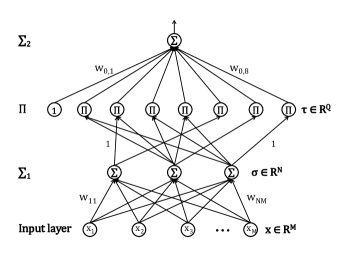
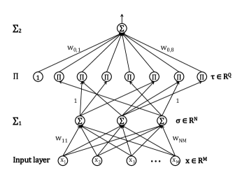
After performing Algorithms 1 with , and , we select eight monomials, , to approximate the complete multinomial. The new structure corresponds to Fig. 3. The new weighted linear combination is
| (29) |
From Fig. 3, the first product node, corresponding to the bias , does not connect with any node in the layer, so And we have
| (30) |
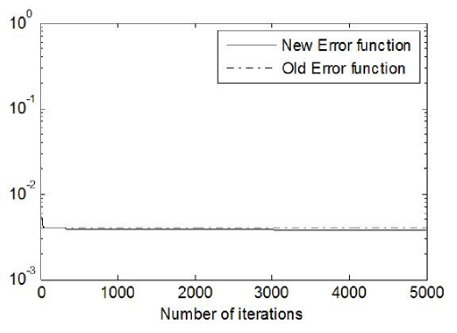
Then, we perform Algorithms 2 and use the test samples to evaluate our method. The average error with different parameter over the 20 tests and the improvement of the performance have been shown in Table 2. The persuasive comparison shows that the new structure attains the best effectiveness, i.e., the smallest error. From Fig. 1, we see that the surface of Mayas’ error function in new structures is monotonically decreasing and converge to 0.
| Learning Rate | Average Old | Average New | Improvement % |
|---|---|---|---|
| 0.001 | 0.0042 | 0.0041 | 2.38 |
| 0.005 | 0.0043 | 0.0040 | 6.98 |
| 0.01 | 0.0040 | 0.0039 | 2.5 |
| 0.05 | 0.0039 | 0.0033 | 15.38 |
| 0.1 | 0.0040 | 0.0035 | 12.5 |
4.2 Example 2: Gabor function approximate
In this example, a MPSPNN is used to approximate the Gabor function as:
| (31) |
The training samples of the neural network are 36 input points selected from an evenly grid on and Similarly, the test samples are 400 input points selected from grid on and . By performing Algorithms 1 with , and , and are selected to approximate the complete multinomial. The new structure corresponds to Fig. 3 and the new weighted linear combination is
| (32) |
and we have
| (33) |
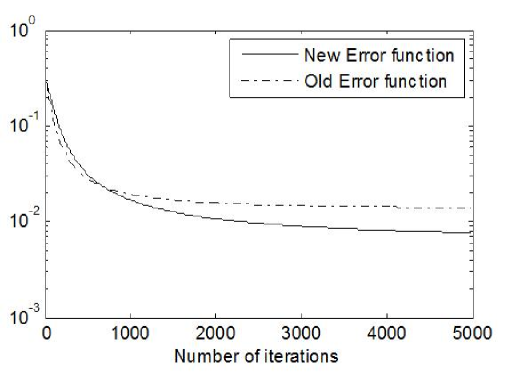
Then, we perform Algorithms 2 and use the test samples to evaluate our method. The average error and the improvement of the performance have been shown in Table 3. The results show that the new structure attains the smallest error. From Fig. 2, we see that the surface of Gabor error function in new structures is monotonically decreasing and converge to 0, as predicted by Theorem 1.
| Learning Rate | Average Old | Average New | Improvement % |
|---|---|---|---|
| 0.001 | 0.0131 | 0.0075 | 42.75 |
| 0.005 | 0.0133 | 0.0065 | 51.13 |
| 0.01 | 0.0130 | 0.0064 | 50.77 |
| 0.05 | 0.0132 | 0.0063 | 52.27 |
| 0.1 | 0.0131 | 0.0055 | 58.02 |
4.3 Example 3: Sonar data classification
Sonar problem is a well-known benchmark dataset, which aims to classify reflected sonar signals into two categories (metal cylinders and rocks). The related data set comprises 208 input vectors, each with 60 components. In this example, 4-fold cross validation is used to perform experiments, that is, samples for training and samples for testing are stochastically selected from the 208 samples. After performing our method, and are selected to to approximate the complete multinomial. The new structure corresponds to Fig. 3 and the new weighted linear combination is
| (34) |
Then, we have
| (35) |
| Round | Old Train | New Train | Impprovment% | Old Test | New Test | Improvement% |
|---|---|---|---|---|---|---|
| 1 | 79.42 | 89.26 | 11.67 | 71.16 | 83.18 | 15.58 |
| 2 | 86.22 | 95.67 | 10.39 | 81.02 | 90.74 | 11.32 |
| 3 | 85.12 | 87.51 | 2.77 | 78.85 | 81.73 | 3.59 |
| 4 | 80.77 | 90.87 | 11.77 | 68.52 | 82.85 | 18.93 |
| 5 | 79.97 | 84.94 | 6.03 | 76.28 | 80.45 | 5.32 |
| Overall | 82.30 | 89.65 | 8.67 | 75.17 | 83.79 | 10.85 |
| Round | Old Train | New Train | Impprovment% | Old Test | New Test | Improvement% |
|---|---|---|---|---|---|---|
| 1 | 89.47 | 99.36 | 10.48 | 84.62 | 98.11 | 14.76 |
| 2 | 94.87 | 99.36 | 4.62 | 89.47 | 95.62 | 6.65 |
| 3 | 95.62 | 96.15 | 0.55 | 88.46 | 92.31 | 4.26 |
| 4 | 84.62 | 100.0 | 16.66 | 89.47 | 100.0 | 11.12 |
| 5 | 88.46 | 100.0 | 12.25 | 79.49 | 88.46 | 10.65 |
| Overall | 90.61 | 98.97 | 8.82 | 86.30 | 94.90 | 9.49 |
| Round | Old Train | New Train | Impprovment% | Old Test | New Test | Improvement% |
|---|---|---|---|---|---|---|
| 1 | 71.79 | 80.77 | 11.77 | 57.69 | 69.23 | 18.18 |
| 2 | 73.08 | 91.03 | 21.88 | 71.79 | 84.62 | 16.41 |
| 3 | 73.08 | 78.21 | 6.85 | 61.54 | 65.38 | 6.05 |
| 4 | 71.79 | 75.00 | 4.37 | 50.0 | 71.79 | 35.78 |
| 5 | 75.00 | 78.21 | 4.19 | 71.79 | 78.21 | 8.56 |
| Overall | 72.95 | 80.64 | 10.01 | 62.56 | 73.85 | 16.55 |
In both structures, 20 trials are carried out for each learning algorithm. In Tables 4, 5 and 6, we compare average accuracy, best accuracy and worst accuracy of classification of both structures, respectively. In all three tables, it can be seen that new structure is more advantageous than the old structure. These show that our new structure is better and monotonically decreasing and converge to 0 during the iterative learning as predicted by Theorem 1.
4.4 Example 4: Pima Indians diabetes data classification
To verify the theoretical evaluation of MSPSNNs, we used a Pima Indians Diabetes Database, which comprises 768 samples with 8 attributes. The dataset is available at UCI machine learning repository (http://archive.ics.uci.edu/ml/datasets/Pima+Indians+Diabetes). 4-fold cross validation is used to perform our method.
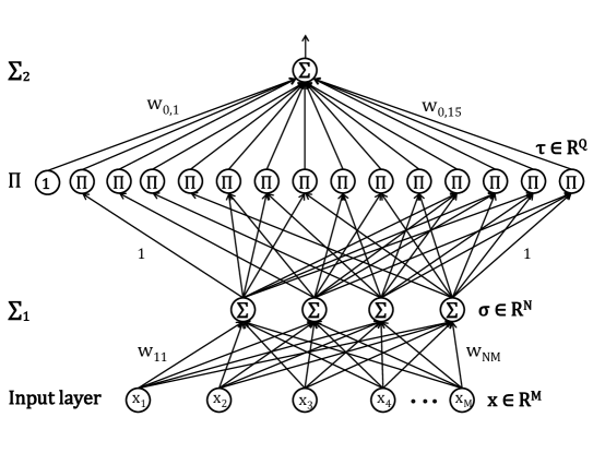
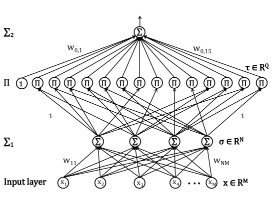
After that, are selected. The new structure corresponds to Fig. 5 and the new weighted linear combination is
| (36) |
Then, we have
| (37) |
The results of comparative analysis experiments using old and new structure for four-order are also presented, paying particular attention to average error, average best error and average wort correct classification shown in Tables 6, 7 and 8. These lead to verify the theoretical evaluation of SPSNNs learning with new structure is better and monotonically decreasing and converge to 0 during the iterative learning as predicted by Theorem 1.
| Round | Old Train | New Train | Impprovment% | Old Test | New Test | Improvement% |
|---|---|---|---|---|---|---|
| 1 | 78.76 | 82.53 | 4.67 | 72.31 | 77.57 | 7.02 |
| 2 | 73.04 | 79.38 | 8.32 | 68.24 | 84.62 | 9.2 |
| 3 | 84.33 | 84.70 | 0.44 | 79.44 | 65.38 | 0.24 |
| 4 | 81.01 | 85.81 | 5.75 | 75.86 | 71.79 | 4.18 |
| 5 | 75.97 | 81.22 | 6.68 | 71.52 | 78.21 | 5.89 |
| Overall | 78.62 | 82.73 | 5.09 | 73.47 | 77.4 | 7.79 |
| Round | Old Train | New Train | Impprovment% | Old Test | New Test | Improvement% |
|---|---|---|---|---|---|---|
| 1 | 88.13 | 89.39 | 1.42 | 76.67 | 786.61 | 12.18 |
| 2 | 77.01 | 85.97 | 11.0 | 74.58 | 78.75 | 5.44 |
| 3 | 89.17 | 91.37 | 2.44 | 85.97 | 88.06 | 2.40 |
| 4 | 87.08 | 90.00 | 3.30 | 81.53 | 83.93 | 2.90 |
| 5 | 78.75 | 83.76 | 6.17 | 75.63 | 79.70 | 5.24 |
| Overall | 84.03 | 88.10 | 4.73 | 78.88 | 83.41 | 5.70 |
| Round | Old Train | New Train | Impprovment% | Old Test | New Test | Improvement% |
|---|---|---|---|---|---|---|
| 1 | 73.61 | 75.41 | 2.42 | 69.74 | 71.59 | 2.62 |
| 2 | 63.49 | 73.0 | 13.94 | 61.98 | 66.76 | 7.43 |
| 3 | 76.04 | 77.08 | 1.36 | 69.44 | 71.40 | 2.78 |
| 4 | 69.44 | 76.04 | 9.07 | 61.98 | 69.44 | 11.35 |
| 5 | 73.96 | 79.44 | 7.2 | 69.44 | 71.98 | 3.59 |
| Overall | 71.31 | 76.19 | 13.0 | 66.52 | 70.23 | 5.43 |
5 Conclusion
In this study, we use the smoothing regularization to automatically select some appropriate terms to approximate the complete Kolmogorov-Gabor Multinomial for the product layer of SPSNNs.Numerical experiments are implemented for Mayas’ function problem, Gabor function problem, Sonar data classification and Pima Indians diabetes data classification. The numerical results demonstrate that the terms, or equivalently the product nodes selected by using smoothing regularization have been proved the capability of providing more possibility powerful mapping, which is different from that in old structure.
References
- [1]
- [2] []
- [3] C.K. Li, A sigma-pi-sigma neural network, Neural Process. Lett. 17 (2003), pp. 1-9.
- [4] Y. Liu, Z. Li, D. Yang, K.S. Mohamed, J. Wang, W. Wu, Convergence of batch gradient learning algorithm with smoothing regularization for Sigma-pi-sigma neural networks. Neurocomputing 151 (2015), pp. 333-341.
- [5] M.M. Gupta, N. Homma, Z.G. Hou, M.G. Solo, I. Bukovsky, Higher order neural networks: fundamental theory and applications. Artificial Higher Order Neural Networks for Computer Science and Engineering: Trends for Emerging Applications pp. 397-422, 2010.
- [6] D.E. Rumelhart, G.E. Hinton, R.J. Williams, (1985) Learning internal representations by error propagation (No. ICS-8506). California Univ San Diego La Jolla Inst for Cognitive Science.
- [7] G.P. Liu, (2012) Nonlinear identification and control: a neural network approach. Springer Science Business Media.
- [8] M.Fallahnezhad,M.H. Moradi,S. Zaferanlouei, (2011) A hybrid higher order neural classifier for handling classification problems. Expert Systems with Applications, 38(1), 386-393.
- [9] A. R. barron, Predicted Squared Error: A criterion for automatic model selection,” Self-Organizing Methods in Modeling: GMDH Type Algorithms (S.J. Farlow, Ed.), Marcel Dekker, Inc., NY, Chap.4 (1984), pp. 87-103.
- [10] V. S. Stometta and B. A. Hubermann, An improved three-layer back propagation algorithm, in Proc. IEEE IJCNN, vol. 2, (1987), pp.637-643.
- [11] H. Zhang, Y. Tang, X. Liu, (2015) Batch gradient training method with smoothing regularization for feedforward neural networks. Neural Computing and Applications, 26(2), 383-390.
- [12] W. Wu, Q.W. Fan, J.M. Zurada et al., Batch gradient method with smoothing regularization for training of feedforward neural networks,Neural Networks 50 (2014) 72-78.
- [13] R. Reed, Pruning algorithms-a survey,IEEE Transactionson Neural Networks 8 (1997) 185-204.
- [14] S. Shalev-Shwartz, T. Zhang, (2014) Accelerated proximal stochastic dual coordinate ascent for regularized loss minimization. In International Conference on Machine Learning (pp. 64-72).
- [15] J. Tang, S. Alelyani, H. Liu, (2014) Feature selection for classification: A review. Data Classification: Algorithms and Applications, pp. 37.
- [16] S. Scardapane, D. Comminiello, A. Hussain, et al. (2017) Group sparse regularization for deep neural networks. Neurocomputing 241:81-89.
- [17] Z. Xu, H. Zhang, Y. Wang, X. Chang, regularization, Science ChinaInformation Sciences, Vol. 53, No. 6 (2010) pp. 1159-1165.
- [18] W. Wu, H. Shao, Z. Li, Convergence of batch BP algorithm with penalty for FNN training, in Neural Information Processing, (2006) 562-569.
- [19] J. Wang, W Wu, J. M. Zurada, 2012, Computational properties and conver-gence analysis of BPNN for cyclic and almost cyclic learning with penalty, Neural Networks, Vol. 33, pp. 127-135.
- [20] A. S. Weigend, D. E. Rumelhart, B. Huberman, Generalization by weight-elimination applied to currency exchange rate prediction, in Neural Networks, IJCNN 1991 International Joint Conference on, Seattle, (1991), PP.837-841.
- [21] Z. Xu, X. Chang, F. Xu, H. Zhang, Regularization: A Thresholding Representation Theory and a Fast Solver, Neural Networks and Learning Sys-tems, IEEE Transactions on, Vol. 23, No. 7, (2012) pp. 1013-1027.
- [22] M. Yuan, Y. Lin, Model selection and estimation in regression with grouped variables, Journal of the Royal Statistical Society: Series B (Statistical Methodology), Vol. 68 (2006) pp. 49-67.
