Single Image Reflection Removal Using Deep Encoder-Decoder Network

Abstract

Image of a scene captured through a piece of transparent and reflective material, such as glass, is often spoiled by a superimposed layer of reflection image. While separating the reflection from a familiar object in an image is mentally not difficult for humans, it is a challenging, ill-posed problem in computer vision. In this paper, we propose a novel deep convolutional encoder-decoder method to remove the objectionable reflection by learning a map between image pairs with and without reflection. For training the neural network, we model the physical formation of reflections in images and synthesize a large number of photo-realistic reflection-tainted images from reflection-free images collected online. Extensive experimental results show that, although the neural network learns only from synthetic data, the proposed method is effective on real-world images, and it significantly outperforms the other tested state-of-the-art techniques.

1 Introduction

Photographing a scene behind a transparent medium, most commonly glasses, tends to be interfered by the reflections of the objects on the side of the camera. The intended reflection-free image, which we call the transmission image $T$, becomes intertwined with the reflection image $R$, and is consequently recorded as a mixture image $I$. The reflections cause annoying image degradations of arguably the worst kind and make many computer vision tasks, such as segmentation, classification, recognition, etc., very difficult if not impossible. For a range of important applications, the separation and removal of reflection image $R$ from the acquired mixture image $I$ is a challenging image restoration task out of necessity.

Figure 1: The proposed reflection removal technique separates reflections from a given reflection-interfered image (left) and outputs a clean image (right) without the reflection artifacts.

A widely adopted and satisfactory model for the formation of the mixture image is

$$I=\alpha T+\beta R+n.$$ (1)

where $n$ is the noise term, $\alpha$ and $\beta$ are the transmittance and reflection rate of the glass, respectively; they determine the mixing weights of the two component images. Compared with other image restoration tasks, such as denoising, superresolution, deblurring, etc., reflection removal is far more difficult. The underlying inverse problem is one of blind source separation and it is more severely underdetermined as there are not one but two unknown images $T$ and $R$ that need to be estimated from the observed image $I$. Adding to the level of difficulty is that both component signals $T$ and $R$ are natural images of similar statistics.

Many researchers have taken on the technical challenge of reflection removal and proposed a number of solutions for the problem. But the current state of the art is still quite limited in terms of the performance, robustness and generality. One approach is the use of specially designed optical devices, such as polarizing filters, to obtain a series of perfectly aligned images with different levels of reflections for layer separation [19]. Although such optical devices make the reflection removal problem easier to tackle, they incur additional hardware costs, reduce light influx, and have limited scope of applications. Thus, many techniques use multiple images of the targeted scene taken from slightly different viewing positions instead to get varied reflections [10, 23]. However, as these techniques require accurate image registration, they are only applicable when the imaged objects are relatively flat and not in motion.

Ideally, a reflection removal algorithm should work with a single mixture image, albeit a daunting task. Some attempts have been reported in the literature on single-image reflection removal [22, 7]. In these papers, the authors adopted the image formation model of Eq. (1) and formulated the problem as the decomposition of the observed mixture image $I$ into two components $T$ and $R$ of different characteristics. In order to separate the reflection from the transmission, they all made some explicit assumptions about the reflection image $R$ so it can be distinguished from the transmission image $T$. For instance, Shih et al. proposed to use the double image caused by the two surfaces of the glass to identify reflection [35]. But unless the camera is close to the glass, the double image effect is too insignificant to be useful. Other techniques also try to exploit the smoothness and sparsity of the reflection layer [24]. However, transmission image can have smooth and sparse regions as well, making these priors non-discriminative.

Apparently, the task of single image reflection removal has been greatly hindered by the inability of conventional statistical models to separate reflection and transmission images. We humans can, on the other hand, mentally separate the two images although being visually disturbed. The difference lies in that humans can perform the separation task largely relying on the coherence of high-level semantics of the two images, while existing models cannot. This suggests that machine learning is a sensible and promising strategy for overcoming the persistent difficulties in removing reflections based on a single mixture image. Furthermore, the machine learning approach, with properly chosen training data, can also circumvent the obstacle of grossly ill conditioning in solving the problem directly using the image formation model of Eq. (1), in which the number of unknowns greatly exceeds the number of equations.

In this paper, instead of using an explicit model like most existing techniques, we propose a data-driven approach based on deep convolutional neural network (CNN) for removing reflections in a single image as shown in Figure 1. Similar to many CNN based image restoration techniques for problems like inpainting, denoising and superresolution, the proposed approach recovers a reflection-free image from a given image by learning an end-to-end mapping of image pairs with and without reflections. To fully exploit the fact that the reflection image, the addictive “noise” to be removed, is also a natural image as discussed previously, we design a novel three-stage deep encoder-decoder network that first estimates the reflection layer and then reconstructs a high quality transmission layer based on the estimated reflection and perceptual merits. Due to the difficulty of obtaining a sufficiently large set of real image pairs for training the neural network, we carefully model the physical formation of reflection and synthesize a large number of photo-realistic reflection-tainted images from reflection-free images collected online. Extensive experimental results show that the neural network can generalize well using only synthesized training data and significantly outperform other tested techniques for real-world images.

The remainder of the paper is organized as follows. Section 2 provides an overview of related work in the literature. In Section 3 we introduce our method for synthesizing training data, and in Section 4 we present in detail our proposed method. Section 5 shows the experiment evaluations of the proposed method with both synthetic and real-world images. Finally, Section 6 concludes.

2 Related Work

Many existing reflection removal methods rely on two or more input images of the same scene with different reflections to estimate the transmission layer. To obtain such images of varied reflections, several photography techniques can be used. Some reflection removal methods employ polarizing filter to manipulate the level of the reflections [27, 8, 30]. The physically-based method proposed by Schechner et al. shows the advantages of using orthogonal polarized input images [34]. Kong et al. further improve this idea by exploiting the spatial properties of polarization [19]. Similar to polarizing filtering, flash lighting [9, 2] and defocus blurring [33, 32] can help generate images with varied reflections without moving the camera as well. Keeping the camera relatively stationary is crucial to the efficacy of these device-based reflection removal techniques, as if the objects behind the glass are also not in motion, the only changing components among the input images are the reflections while the transmission layer is invariant.

There are also many multi-image techniques that exploit the motion of the camera as a cue for reflection removal. These techniques first align the objects in a series of images taken from slightly different viewing positions and then separate the invariant layer as the reflection-free image [39, 10]. To align images interfered by reflections, Tsin et at. [40] and Sinha et al. [38] use efficient stereo matching algorithms. Guo et al. exploit the sparsity and independence of the transmission and reflection layers to improve the robustness of image alignment [12]. Off-the-shelf optical flow algorithms are also employed for aligning images [23, 13]. With motion smoothness constraints, optical flow techniques can be more accurate and robust for the layer separation task [45, 46]. For the cases where the camera is stationary while the objects are moving, the reflection layer is relatively static and must be handled differently [31, 36].

If only one image of the scene is given, which is the case tackled by this paper, the task of reflection removal becomes much more challenging. Only a few single image reflection removal techniques have been reported in the literature. Many of these techniques still rely on some extra information provided by light field camera [6, 26] or the user [21, 48]. One of the first attempts to solve the problem without any user assistance is [22], which minimizes the total amount of edges and corners in the two decomposed layers of the input image. Akashi et al. [3] employ sparse non-negative matrix factorization to separate the reflection layer without a explicit smoothness prior. The work of Li and Brown [24] assumes that the reflection layer is smoother than the transmission layer due to defocus blur and hence has a short tail gradient distribution. With a similar smoothness assumption for the reflection layer, Fan et al. [7] use two cascaded CNN networks to reconstruct a reflection reduced image from the edges of the input image. Arvanitopoulos et al. [5] formulate the reflection suppression problem as an optimization problem with a Laplacian data fidelity term and a total variation term. Wan et al. [42] combine the sparsity prior and nonlocal prior of image patches in both the transmission and reflection layers together. They further increase the effectiveness of the nonlocal prior using image patches retrieved from an external dataset. The work of Shih et al. [35] takes advantage of ghosting, the phenomenon of multiple reflections caused by thicker glass, and decomposes the input image based on Gaussian mixture model (GMM). To deal with reflections from eyeglasses in frontal face image, Sandhan and Choi [29] exploit the bilateral symmetry of human face and use a mirrored input image as another input of varied reflections.

For more detailed review on the existing techniques for reflection removal, we refer readers to two excellent surveys [4] and [41].

3 Preparation of Training Data

The proposed technique recognizes and separates reflections from the input image using an end-to-end mapping trained by image pairs with and without reflections. The effectiveness of our technique, or any machine learning approaches, greatly relies on the availability of a representative and sufficiently large set of training data. In this section, we discuss the methods for collecting and preparing the training images for our technique.

To help the proposed technique identify the patterns of reflections in real-world scenarios, ideally, the training algorithm should only use real photographs as the training data. Obtaining an image with real reflections is not difficult; we can capture such a mixture image $I$, as in Eq. (1), by placing a piece of reflective glass of transmittance $\alpha$ in front of the camera. The corresponding clean image $T$ of the same scene is also attainable using the same camera setup but without the glass. However, training images collected using this scheme have several non-negligible drawbacks and limitations. First, it is almost impossible to get a pair of images that are perfectly aligned. Even with a tripod that stabilizes the camera, the motions of objects within the scene can still cause misalignment between two images captured consecutively.

Furthermore, due to the effects of refraction, the glass shielding the scene shifts the path of light transmitting through the glass and can also lead to the alignment problem. By the reflection formation model in Eq. (1), these differences introduced by the misalignment between the mixture image $I$ and its reflection-free counterpart $T$ can be seen as a part of the noise term $n$, where

$$\beta R+n=I-\alpha T.$$ (2)

Since the noise introduced by misalignment has similar characteristics as a natural image, it is difficult to accurately distinguish the noise $n$ from the reflection image $\beta R$. As a result, a training algorithm could erroneously attribute part of the noise $n$ as the effects of the reflection $\beta R$, interfering the learning of the true reflections. Similarly, regional illumination changes between a pair of images can lead to the increase of structural noise in training data as well. Although it is possible to reduce these adverse effects by carefully shooting only static scene from a stationary camera or using thinner reflective glass with small refraction, these methods greatly limit the flexibility and practicality of collecting real images as training data.

Due to the unavoidable limitations discussed above and the prohibitive cost of building a large enough training set of real images, we use synthetic images constructed from images collected online for training instead. The main idea of the synthesis process follows the physical reflection formation model in Eq. (1), which interprets a reflection-interfered image $I$ as the linear combination of two reflection-free natural images $T,R$. The formation model, however, cannot be applied directly to most of the JPEG-compressed images available online. The reason is that, to take advantage of human’s non-linear light sensitivity, JPEG images have to be gamma corrected before being stored on camera, hence their pixel values are not linear to the light intensities captured by image sensor. Consequently, the direct summation of two gamma-corrected images does not conform the physics of light superposition as required by Eq. (1), resulting unrealistic reflection-interfered image. To correct this problem, we can either only use raw image or apply inverse gamma correction on the collected JPEG images, as follows

$$X=(X^{\prime})^{1/\gamma},$$ (3)

where $X^{\prime}$ is a gamma corrected image and $X$ is the corresponding light intensity image. The gamma correction coefficient $\gamma$ for each color channel is often available in exchangeable image file format (EXIF) segment attached in each JPEG image. In the following discussion, we still use the linear formula as in Eq. (1) and assume that all the pixel values are restored to the raw light intensity readings from image sensor.

To accurately simulate the formation of reflection-interfered image, we also consider the blur effect in the reflections. In most real images, the focal planes of the camera are on the objects behind the glass rather than the reflected objects, since what behind the reflective glass are normally the objects of interest. As a result, reflections are often blurry due to the defocus effect [24, 7]. To simulate this effect in the synthetic image, we blur the reflection image $R$ with a Gaussian kernel $G$ of random variance before superimposing it into the synthetic image $I_{B}$, as follows,

$$I_{B}=\alpha T+\beta R*G$$ (4)

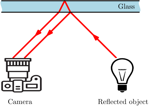
Figure 2: The formation of double reflection.

In addition to the reflection blurring, we also consider the double reflection effect in synthesized image. Double reflection effect is formed due to the reflections from the two surfaces of the reflective glass as shown in Fig. 2. The offset between the two reflection images are decided by the relative position and angle of the camera and the reflective glass. Suppose the transmittance of the glass is $\alpha$ and its reflectivity is $1-\alpha$, then the strengths of the double reflections are approximately $1-\sqrt{\alpha}$ and $\sqrt{\alpha}-\alpha$, respectively. This reflection effect can be simulated by convoluting the reflection image $R$ with a random kernel $K$ with two pulses of amplitude $1-\sqrt{\alpha}$ and $\sqrt{\alpha}-\alpha$.

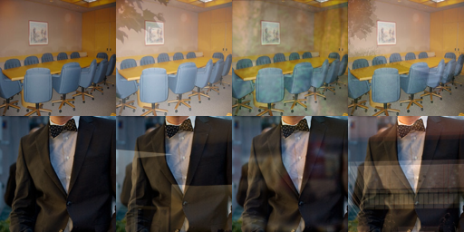
Figure 3: Samples of synthesized images. From left to right: Transmission images, synthetic images with sharp reflections, synthetic images with blurry reflections, synthetic images with double reflections

Combining the blurring and double reflection effects together, we arrive at a generic formula for synthesizing reflection-interfered image $I$.

$$I=\alpha T+\beta R*G*K.$$ (5)

Some samples of synthesized images are shown in Figure 3.

4 Proposed Method

4.1 Network Architecture

Similar to many deep learning based image restoration techniques, the proposed reflection removal method adopts the basic architecture of a convolutional encoder-decoder network [25]. The ultimate goal of our method is to find an optimal end-to-end mapping $T^{\prime}=F(I)$ from a reflection-interfered image $I=T^{\prime}+R^{\prime}$ to its transmission layer $T^{\prime}$, where $R^{\prime}$ is the reflection layer of $I$. The transmission layer $T^{\prime}=\alpha T$ is a glass-free image $T$ of the targeted scene attenuated by $\alpha$, the transmittance of the reflective glass in image $I$, as in the training data synthesis formula Eq. 5. Since the reflection layer $R^{\prime}$ is likely weak and smooth in comparison with $T^{\prime}$ [24, 5], $T^{\prime}$ should be similar to $I$ in pixel values. Therefore, it is easier to optimize mapping $T^{\prime}=F(I)$ than to optimize the mapping from $I$ to $T$ directly, even if transmittance $\alpha$ is known to the network. Once the solution to the transmission layer $T^{\prime}$ is given, it is trivial to restore a realistic reflection free image $T$ from $T^{\prime}$.

Another option is to train a residual mapping from image $I$ to its reflection layer $R^{\prime}=I-F(I)$. Since $R^{\prime}$ is relatively flat, the optimization of the residual mapping should be very effective. Residual learning has set the state of the art for many different image restoration problems [20, 17, 14]. However, none of the existing residual learning networks suits the characteristics of the reflection removal problem. In most residual learning techniques, the residual is the missing detail to be recovered and added back to the input image, while in our case, the residual is unwanted reflection that should be subtracted from the input. Furthermore, residual learning tends to emphasize on the fidelity of the recovered residual as the loss function is normally applied on the residual. But for the reflection removal problem, as long as the recovered transmission layer has reduced interference and looks natural, the restoration quality of the reflection layer is irrelevant. Due to these limitations, it is difficult to get satisfactory results for reflection removal by using residual learning directly. Thus, we place a residual learning based reflection recovery sub-network at the middle of our end-to-end mapping $T^{\prime}=F(I)$ network, in order to exploit the efficiency of residual learning without affecting the output quality.

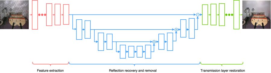
Figure 4: Architecture of the used convolutional auto-encoder with symmetric shortcut connection.

(a) Synthetic input
 

(b) Recovered reflection image

(c) Recovered transmission image

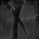
(d) $\mathit{conv}_{2}$

(e) $\mathit{conv}_{4}$

(f) $\mathit{conv}_{6}$

(g) $\mathit{deconv}_{2}$

(h) $\mathit{deconv}_{4}$

(i) $\mathit{deconv}_{6}$

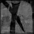
(j) $\mathit{deconv}_{7}$

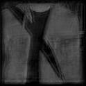
(k) $\mathit{deconv}_{9}$

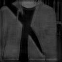
(l) $\mathit{deconv}_{11}$

Figure 5: Sample feature maps at different stages of the network. These feature maps show that the network is working as intended in each stage.

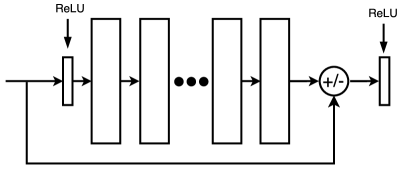
Figure 6: The topology of a single shortcut connection.

The proposed network consists of 12 convolutional layers and 12 deconvolutional with one rectified linear unit (ReLU) following each of the layers. The convolutional layers are designed to extract and condense features from the input, while deconvolutional layers rebuild the details of reflection-free image from feature abstractions. Overall, the architecture of proposed encoder-decoder network can be divided into three stages:

1. Feature extraction. The 6 convolutional layers in this stage extract features for both transmission and reflection layers as illustrated in Figure 4. The outputs of the convolutional layers are shown in the second row of Figure 5.

2. Reflection recovery and removal. In this stage, the first 6 convolutional layers and following 6 deconvolutional layers are set to learn and recover reflection. Additionally, to preserve the details of the reflection layer better, two skip connections are added in the second stage to inherit the features learned from previous convolutional layers [25]. The topology of skip connection is illustrated in Figure 6. At the end of this stage, the recovered reflection is removed before $\mathit{deconv}_{7}$, the seventh deconvolutional layer, by using an element-wise subtraction [47] followed by a ReLU activation $\max(0,\mathit{conv}_{6}\!-\!\mathit{deconv}_{6})$. As shown in the third row of Figure 5, this stage removes the transmission layer gradually from the input and preserves only the features of the reflections.

3. Transmission layer restoration. The reflections might not be removed completely after previous stage by simply subtracting the estimated reflection, as shown in the last row of Figure 5. Thus, this stage tries to restore a visually pleasing transmission image from the reflection subtracted image. To achieve this goal, 6 deconvolutional layers are used to recover transmission layer from the features of the targeted scene.

For image classification tasks, pooling layers are necessary as it extracts main abstract features that are crucial for final decision [14]. However, as the redundant information increases the difficulty for deconvolutional layers to recover the image [25], pooling layers are omitted in our reflection removal network. Another important factor that affects the performance of our encoder-decoder network is the size of the convolutional kernel. To make the network learn the semantic context of an image, we employ relatively large kernels ($5\times 5$). But if the input image contains double reflections of large disparity, we find a larger kernel ($9\times 9$) for the first convolutional layers ($\mathit{conv}_{1}$ and $\mathit{conv}_{2}$) and the last deconvolutional layers ($\mathit{deconv}_{11}$ and $\mathit{deconv}_{12}$) is necessary to achieve the best performance.

4.2 Loss functions

In many neural network based image restoration techniques, such as denoising [43], debluring [44] and super resolution [17], the networks are commonly optimized using mean square error (MSE) between the output and the ground truth as the loss function,

$$L_{\ell_{2}}=\|F(I)-\alpha T\|_{2}^{2}$$ (6)

However, a model optimized using only $\ell_{2}$-norm loss function often fails to preserve high-frequency contents. In the case of reflection removal, both the reflection and transmission layers are natural images with different characteristics. To get the best restoration result, the network should learn the perceptual properties of the transmission layer. Inspired by [11, 15], we employ a loss function that is closer to high-level feature abstractions. Based on Ledig et al. [20], the VGG loss is calculated as the $\ell_{2}$-norm of the difference between the layer representations of the restored transmission $T^{\prime}=F(I)$ and the real transmission image $\alpha T$ on the pre-trained 19 layers VGG network proposed by Simonyan and Zisserman [37]:

$$L_{\text{VGG}}=\frac{1}{W_{i}H_{i}}\sum_{i=1}^{M}\|\phi_{i}(\alpha T)-\phi_{i}(F(I))\|_{2}^{2}$$ (7)

where $\phi_{i}$ is the feature maps obtained by the $i$-th convolution layer (after activation) within the VGG19 network; $M$ is the number of convolution layers used; and $W_{i}$ and $H_{i}$ are the dimension of $i$-th feature map. In our model, the feature maps of the first 5 convolution layers are used ($M=5$) to build the perceptual loss. The final loss for training is calculated as:

$$L=L_{\ell_{2}}+\lambda L_{\text{VGG}},$$ (8)

where $\lambda$ is a parameter for balancing the contributions from the $\ell_{2}$-norm loss and the VGG loss.

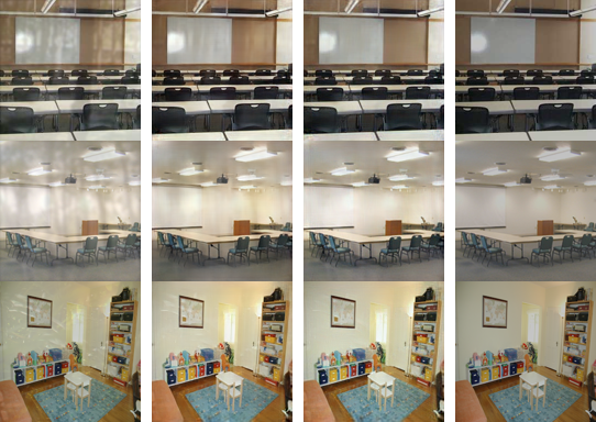
Figure 7: From left to right: input reflection-interfered images, network optimized for $\ell_{2}$-norm loss, network optimized for both $\ell_{2}$-norm and VGG losses, the ground-truth transmission images.

Figure 7 presents some of the results from two reflection removal models trained with loss functions in Eqs. (6) and (8) respectively. As shown in the figure, the output images (3rd column) from the model trained with the mixed loss function as in Eq. (8) is much cleaner and closer to the ground-truths (4th column) than those output images (2nd column) from the model trained solely with $\ell_{2}$-norm loss as in Eq. (6).

5 Experiments

In this section, we first discuss how the training sets are formed and how the parameters are set for training the network. Then, we evaluate the proposed method using synthetic and real images and compare our results with several state-of-art methods.

(a) Synthetic input

(b) [5]

(c) [7]

(d) Ours

(e) Ground truth

Figure 8: Comparison of reflection removal algorithms using synthetic images.

5.1 Data Preparation

To simulate the scenarios where reflections interfere the formation of images, 2303 images from the indoor scene recognition dataset [28] and 2622 street snap images [16] are collected online. We choose the images of natural landscapes and images taken inside a mall as the reflections. Leaves could create sparse shadow on the window interfering the transmission image, and the lights from a shop sign create strong and sharp reflection, which are also extremely common in real life reflection-interfered images. To ensure the size of training dataset and avoid over-fitting, each transmission image is synthesized with 18 randomly chosen reflection images using Eq. (5). To simulate the different blurriness of the reflections, the variance of the Gaussian blur kernel is selected randomly from 1 to 5. The transmittance $\alpha$ is also a random number between 0.75 to 0.8 for each synthetic image. Before generating a synthetic image, the transmission layer is resized to $128\times 128$, whereas the reflection layer is randomly cropped from a large reflection image and then resized to $128\times 128$. The reason for this step is that the reflected objects are normally far away from the glass, as a result, larger objects in the reflection scene appear relatively smaller in the reflection-interfered image. Finally, all the synthesized images are split into a training set of 66540 images and a testing set of 22110 images.

5.2 Network Training

The network is trained in an end-to-end manner as $T^{\prime}=F(I)$ and parametrized by $\theta_{F}$ which donates weights and biases of the network. It is aimed to solve the following objective function:

$$\theta_{F}=\arg\min_{\theta_{F}}\frac{1}{N}\sum_{n=1}^{N}L(F(I_{n}),\alpha T_{n})$$ (9)

where N is the size of training set, $L$ is the combined loss functions defined in Eq. 8. We set 64 filters for all the convolutional and deconvolutional layers and the VGG loss weight $\lambda$ is set to $0.001$. The network is optimized by Adam optimizer [18] with a learning rate of $10^{-4}$ and $\beta_{1}=0.9$, batch size is set to 64 to accelerate the training process. The network is trained for 150 epochs. All the experiments are done on a NVIDIA TITAN X GPU and implementation is based on Tensorflow [1].

(a) Input

(b) [5]

(c) [7]

(d) Ours

(e) Input

(f) [5]

(g) [7]

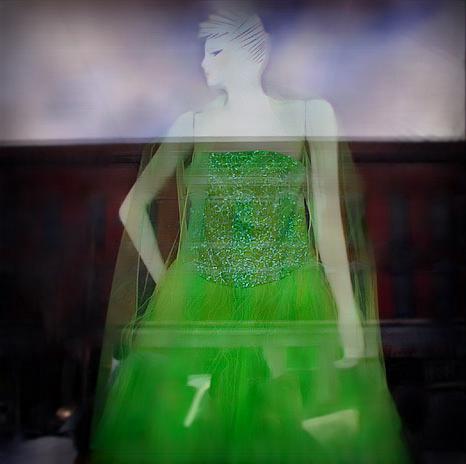
(h) Ours

 

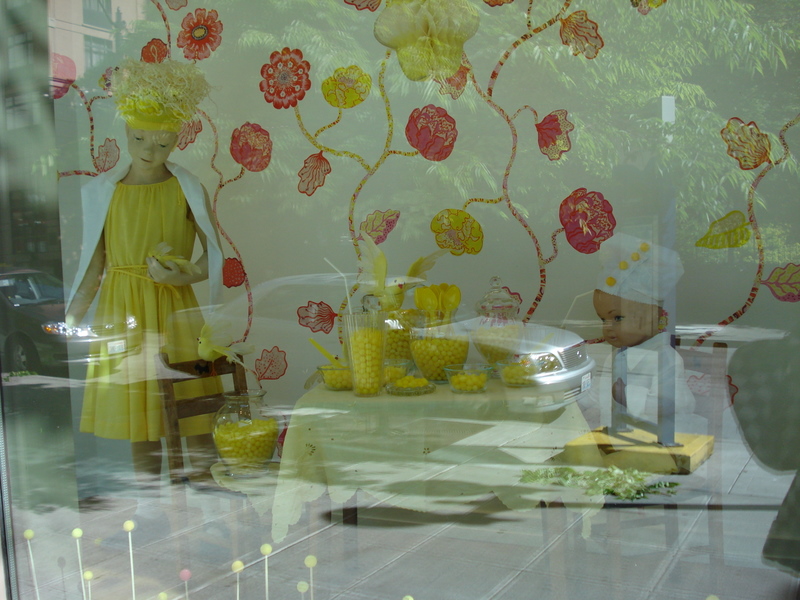
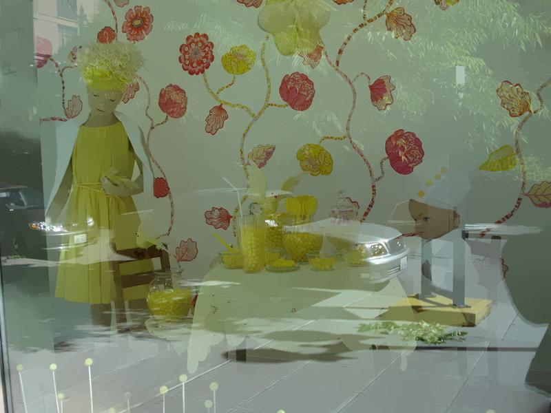
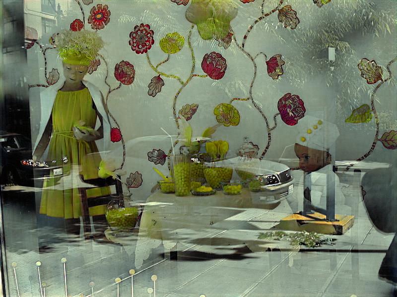
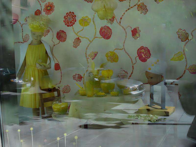
(i) Input

(j) [5]

(k) [7]

(l) Ours

Figure 9: Comparison of reflection removal algorithms using real images.

5.3 Evaluation

Figure 8 shows some results of the proposed method in comparison with the results of two state-of-the-art reflection removal techniques [5] and [7] using synthetic data. It is expected that the proposed method significantly outperforms the compared techniques in this case, as our network is trained with similar images generated by the data synthesizer. For real-life images collected by us or provided by the authors of [5], the results of proposed method are still the best among the tested techniques, as shown in Figure 9. The technique in [7] is based on the assumption that the reflection is smooth. However, if this assumption is not true, as exemplified in the sample images, [7] could even enhance the reflections, making the results worse than the inputs. Our method does not rely on such an assumption; it works well regardless the smoothness of the reflections. The problem of [5] is the severe loss of details in its output, resulting unnatural looking image. In the cases where the reflections are much stronger than the transmission layer, none of the tested algorithms can yield satisfactory results.

	[5]	[7]	Ours
Synthetic Images	19.72	19.82	29.08
Benchmark Set [41]	16.85	18.29	18.70

Table 1: PSNR results of tested techniques using synthetic images and a benchmark dataset.

Reported in Table 1 are the PSNR results of the tested techniques. In addition to the synthetic images, we tested a synthetic benchmark set provided by the authors of [41]. Our method achieves the highest average PSNR in these tests. The running times of the proposed method are comparable to other deep learning based image restoration techniques. The proposed method takes around 0.6 s to process a $128\times 128$ image and 2 s to process a $512\times 512$ image.

6 Conclusion

The task of removing reflection interference from a single image is a highly ill-posed problem. We propose a new reflection formation model taking into the consideration of physics of digital camera imaging, and apply the model in a deep convolutional encoder-decoder network based data-driven technique. Extensive experimental results show that, although the neural network learns only from synthetic data, the proposed method is effective on real-world images, and it significantly outperforms the other tested state-of-the-art techniques.

References

- [1] M. Abadi, A. Agarwal, P. Barham, E. Brevdo, Z. Chen, C. Citro, G. S. Corrado, A. Davis, J. Dean, M. Devin, S. Ghemawat, I. Goodfellow, A. Harp, G. Irving, M. Isard, Y. Jia, R. Jozefowicz, L. Kaiser, M. Kudlur, J. Levenberg, D. Mané, R. Monga, S. Moore, D. Murray, C. Olah, M. Schuster, J. Shlens, B. Steiner, I. Sutskever, K. Talwar, P. Tucker, V. Vanhoucke, V. Vasudevan, F. Viégas, O. Vinyals, P. Warden, M. Wattenberg, M. Wicke, Y. Yu, and X. Zheng. TensorFlow: Large-scale machine learning on heterogeneous systems. http://tensorflow.org/, 2015.
- [2] A. Agrawal, R. Raskar, S. K. Nayar, and Y. Li. Removing photography artifacts using gradient projection and flash-exposure sampling. ACM Transactions on Graphics (TOG), 24(3):828–835, 2005.
- [3] Y. Akashi and T. Okatani. Separation of reflection components by sparse non-negative matrix factorization. In Asian Conference on Computer Vision (ACCV), pages 611–625, 2014.
- [4] A. Artusi, F. Banterle, and D. Chetverikov. A survey of specularity removal methods. Computer Graphics Forum, 30(8):2208–2230, 2011.
- [5] N. Arvanitopoulos Darginis, R. Achanta, and S. Süsstrunk. Single image reflection suppression. In IEEE Conference on Computer Vision and Pattern Recognition (CVPR), 2017.
- [6] P. Chandramouli, M. Noroozi, and P. Favaro. Convnet-based depth estimation, reflection separation and deblurring of plenoptic images. In Asian Conference on Computer Vision (ACCV), pages 129–144, 2016.
- [7] Q. Fan, J. Yang, G. Hua, B. Chen, and D. Wipf. A generic deep architecture for single image reflection removal and image smoothing. In Proceedings of the IEEE International Conference on Computer Vision (ICCV), 2017.
- [8] H. Farid and E. H. Adelson. Separating reflections and lighting using independent components analysis. In IEEE Conference on Computer Vision and Pattern Recognition (CVPR), volume 1, pages 262–267, 1999.
- [9] R. Feris, R. Raskar, K.-H. Tan, and M. Turk. Specular reflection reduction with multi-flash imaging. In Brazilian Symposium on Computer Graphics and Image Processing, pages 316–321, 2004.
- [10] K. Gai, Z. Shi, and C. Zhang. Blind separation of superimposed moving images using image statistics. IEEE Transactions on Pattern Analysis and Machine Intelligence (PAMI), 34(1):19–32, 2012.
- [11] L. Gatys, A. S. Ecker, and M. Bethge. Texture synthesis using convolutional neural networks. In Advances in Neural Information Processing Systems (NIPS), pages 262–270, 2015.
- [12] X. Guo, X. Cao, and Y. Ma. Robust separation of reflection from multiple images. In IEEE Conference on Computer Vision and Pattern Recognition (CVPR), pages 2187–2194, 2014.
- [13] B.-J. Han and J.-Y. Sim. Reflection removal using low-rank matrix completion. In IEEE Conference on Computer Vision and Pattern Recognition (CVPR), pages 5438–5446, 2017.
- [14] K. He, X. Zhang, S. Ren, and J. Sun. Deep residual learning for image recognition. In IEEE Conference on Computer Vision and Pattern Recognition (CVPR), pages 770–778, 2016.
- [15] J. Johnson, A. Alahi, and L. Fei-Fei. Perceptual losses for real-time style transfer and super-resolution. In European Conference on Computer Vision (ECCV), pages 694–711, 2016.
- [16] L. Jokinen and K. Sampo. Hel looks. https://www.hel-looks.com/. [Online; accessed 19-Oct-2017].
- [17] J. Kim, J. Kwon Lee, and K. Mu Lee. Accurate image super-resolution using very deep convolutional networks. In IEEE Conference on Computer Vision and Pattern Recognition (CVPR), pages 1646–1654, 2016.
- [18] D. Kingma and J. Ba. Adam: A method for stochastic optimization. arXiv preprint arXiv:1412.6980, 2014.
- [19] N. Kong, Y.-W. Tai, and J. S. Shin. A physically-based approach to reflection separation: from physical modeling to constrained optimization. IEEE Transactions on Pattern Analysis and Machine Intelligence (PAMI), 36(2):209–221, 2014.
- [20] C. Ledig, L. Theis, F. Huszár, J. Caballero, A. Cunningham, A. Acosta, A. Aitken, A. Tejani, J. Totz, Z. Wang, et al. Photo-realistic single image super-resolution using a generative adversarial network. arXiv preprint arXiv:1609.04802, 2016.
- [21] A. Levin and Y. Weiss. User assisted separation of reflections from a single image using a sparsity prior. IEEE Transactions on Pattern Analysis and Machine Intelligence (PAMI), 29(9):1647–1654, 2007.
- [22] A. Levin, A. Zomet, and Y. Weiss. Separating reflections from a single image using local features. In IEEE Conference on Computer Vision and Pattern Recognition (CVPR), volume 1, pages 306–313, 2004.
- [23] Y. Li and M. S. Brown. Exploiting reflection change for automatic reflection removal. In IEEE International Conference on Computer Vision (ICCV), pages 2432–2439, 2013.
- [24] Y. Li and M. S. Brown. Single image layer separation using relative smoothness. In IEEE Conference on Computer Vision and Pattern Recognition (CVPR), pages 2752–2759, 2014.
- [25] X.-J. Mao, C. Shen, and Y.-B. Yang. Image restoration using convolutional auto-encoders with symmetric skip connections. arXiv preprint arXiv:1606.08921, 2016.
- [26] Y. Ni, J. Chen, and L.-P. Chau. Reflection removal based on single light field capture. In IEEE International Symposium on Circuits and Systems (ISCAS), pages 1–4, 2017.
- [27] N. Ohnishi, K. Kumaki, T. Yamamura, and T. Tanaka. Separating real and virtual objects from their overlapping images. In European Conference on Computer Vision (ECCV), pages 636–646, 1996.
- [28] A. Quattoni and A. Torralba. Recognizing indoor scenes. In IEEE Conference on Computer Vision and Pattern Recognition (CVPR), pages 413–420, 2009.
- [29] T. Sandhan and J. Y. Choi. Anti-glare: Tightly constrained optimization for eyeglass reflection removal. In IEEE Conference on Computer Vision and Pattern Recognition (CVPR), pages 1241–1250, 2017.
- [30] B. Sarel and M. Irani. Separating transparent layers through layer information exchange. In European Conference on Computer Vision (ECCV), pages 328–341, 2004.
- [31] B. Sarel and M. Irani. Separating transparent layers of repetitive dynamic behaviors. In IEEE International Conference on Computer Vision (ICCV), volume 1, pages 26–32, 2005.
- [32] Y. Y. Schechner, N. Kiryati, and R. Basri. Separation of transparent layers using focus. International Journal of Computer Vision (IJCV), 39(1):25–39, 2000.
- [33] Y. Y. Schechner, N. Kiryati, and J. Shamir. Blind recovery of transparent and semireflected scenes. In IEEE Conference on Computer Vision and Pattern Recognition (CVPR), volume 1, pages 38–43, 2000.
- [34] Y. Y. Schechner, J. Shamir, and N. Kiryati. Polarization and statistical analysis of scenes containing a semireflector. Journal of the Optical Society of America A (JOSA A), 17(2):276–284, 2000.
- [35] Y. Shih, D. Krishnan, F. Durand, and W. T. Freeman. Reflection removal using ghosting cues. In IEEE Conference on Computer Vision and Pattern Recognition (CVPR), pages 3193–3201, 2015.
- [36] C. Simon and I. Kyu Park. Reflection removal for in-vehicle black box videos. In IEEE Conference on Computer Vision and Pattern Recognition (CVPR), pages 4231–4239, 2015.
- [37] K. Simonyan and A. Zisserman. Very deep convolutional networks for large-scale image recognition. arXiv preprint arXiv:1409.1556, 2014.
- [38] S. N. Sinha, J. Kopf, M. Goesele, D. Scharstein, and R. Szeliski. Image-based rendering for scenes with reflections. ACM Transactions on Graphics (TOG), 31(4):100:1–100:10, 2012.
- [39] R. Szeliski, S. Avidan, and P. Anandan. Layer extraction from multiple images containing reflections and transparency. In IEEE Conference on Computer Vision and Pattern Recognition (CVPR), volume 1, pages 246–253, 2000.
- [40] Y. Tsin, S. B. Kang, and R. Szeliski. Stereo matching with linear superposition of layers. IEEE Transactions on Pattern Analysis and Machine Intelligence (PAMI), 28(2):290–301, 2006.
- [41] R. Wan, B. Shi, L.-Y. Duan, A.-H. Tan, and A. C. Kot. Benchmarking single-image reflection removal algorithms. In IEEE Conference on Computer Vision and Pattern Recognition (CVPR), pages 3922–3930, 2017.
- [42] R. Wan, B. Shi, A.-H. Tan, and A. C. Kot. Sparsity based reflection removal using external patch search. In IEEE International Conference on Multimedia and Expo (ICME), pages 1500–1505, 2017.
- [43] J. Xie, L. Xu, and E. Chen. Image denoising and inpainting with deep neural networks. In Advances in Neural Information Processing Systems (NIPS), pages 341–349, 2012.
- [44] L. Xu, J. S. Ren, C. Liu, and J. Jia. Deep convolutional neural network for image deconvolution. In Advances in Neural Information Processing Systems (NIPS), pages 1790–1798, 2014.
- [45] T. Xue, M. Rubinstein, C. Liu, and W. T. Freeman. A computational approach for obstruction-free photography. ACM Transactions on Graphics (TOG), 34(4):79:1–79:11, 2015.
- [46] J. Yang, H. Li, Y. Dai, and R. T. Tan. Robust optical flow estimation of double-layer images under transparency or reflection. In IEEE Conference on Computer Vision and Pattern Recognition (CVPR), pages 1410–1419, 2016.
- [47] W. Yang, R. T. Tan, J. Feng, J. Liu, Z. Guo, and S. Yan. Joint rain detection and removal from a single image. arXiv preprint arXiv:1609.07769, 2016.
- [48] S.-K. Yeung, T.-P. Wu, and C.-K. Tang. Extracting smooth and transparent layers from a single image. In IEEE Conference on Computer Vision and Pattern Recognition (CVPR), pages 1–7, 2008.