Dynamics of Driver’s Gaze: Explorations in Behavior Modeling & Maneuver Prediction

Abstract

The study and modeling of driver’s gaze dynamics is important because, if and how the driver is monitoring the driving environment is vital for driver assistance in manual mode, for take-over requests in highly automated mode and for semantic perception of the surround in fully autonomous mode. We developed a machine vision based framework to classify driver’s gaze into context rich zones of interest and model driver’s gaze behavior by representing gaze dynamics over a time period using gaze accumulation, glance duration and glance frequencies. As a use case, we explore the driver’s gaze dynamic patterns during maneuvers executed in freeway driving, namely, left lane change maneuver, right lane change maneuver and lane keeping. It is shown that condensing gaze dynamics into durations and frequencies leads to recurring patterns based on driver activities. Furthermore, modeling these patterns show predictive powers in maneuver detection up to a few hundred milliseconds a priori.

I Introduction

Intelligent vehicles of the future are that which, having a holistic perception (i.e. inside, outside and of the vehicle) and understanding of the driving environment, make it possible for occupants to go from point A to point B safely, comfortably and in a timely manner [1, 2]. This may happen with the driver in full control and getting active assistance from the robot, or the robot is in partial or full control and human drivers are passive observers “ready” to take over as deemed necessary by the machine or human [3, 4]. In the full spectrum from manual to autonomous mode, modeling the dynamics of driver’s gaze is of particular interest because, if and how the driver is monitoring the driving environment is vital for driver assistance in manual mode [5], for take-over requests in highly automated mode [6] and for semantic perception of the surround in fully autonomous mode [7, 8].

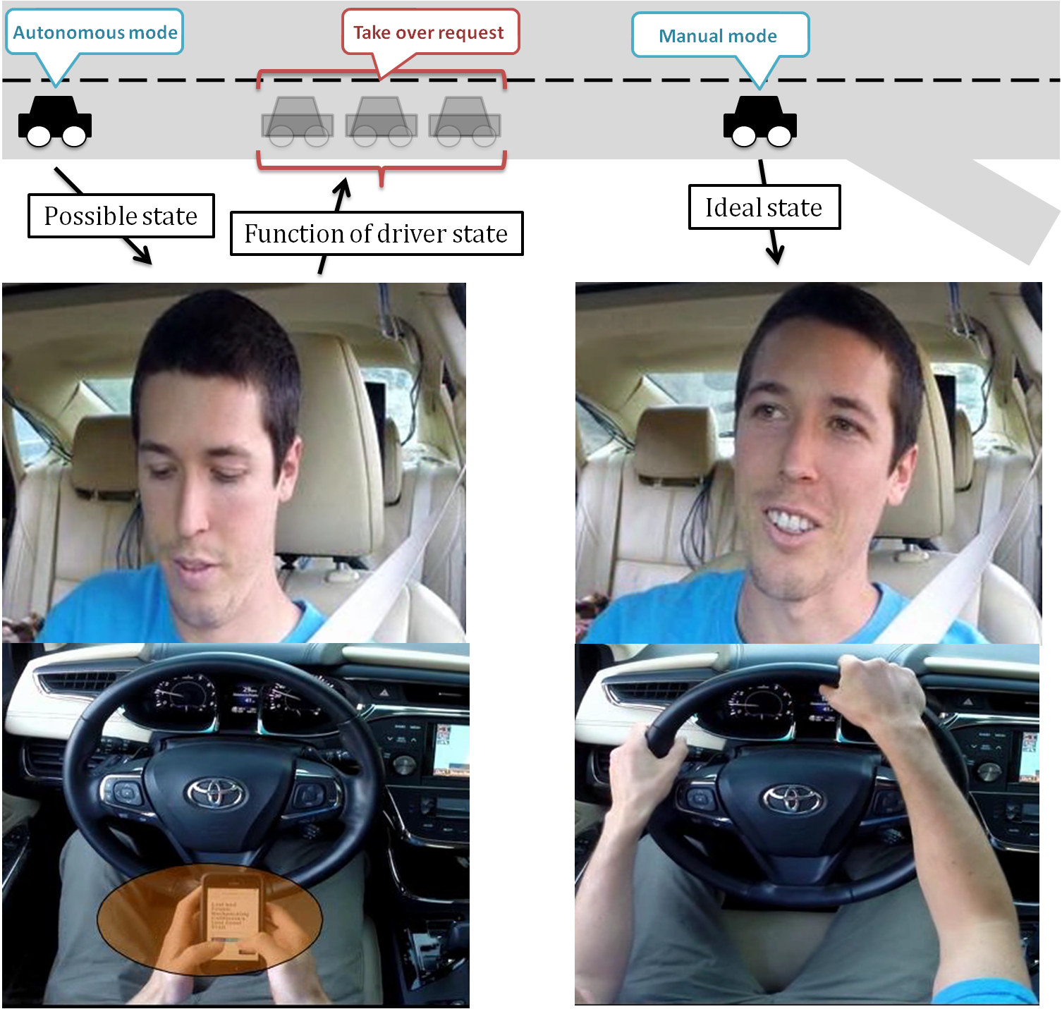
Figure 1: An example illustration which showcases the importance of understanding and modeling what constitutes expected or ”attentive” gaze behavior in order to ensure safe and smooth transfer of control between robot and human.

The driver’s gaze can be represented in many different ways, from directional vectors [9] to points in 3-D space [10], from static zones of interest (e.g. speedometer, side mirrors) [11] to dynamic objects of interest (e.g. vehicles, pedestrians) [12]. In this paper, gaze is represented using context rich static zones of interest. Using such a representation, when gaze is estimated over a period of time, higher semantic information such as fixations and saccades can be extracted and used to derive driver’s situational awareness, estimate engagement in secondary activities, predict intended maneuvers, etc. Figure 1 illustrates an example where the length of driver’s fixation on non-driving relevant region is an important factor to determine driver’s state and therefore, when the transfer of control should happen.

In general, with rapid introductions of autonomous features in consumer vehicles, there is a need to understand and model what constitutes “normal” or “attentive” gaze behavior in order to ensure safe and smooth transfer of control between robot and human. An important criteria to build such models is naturalistic driving data, where driver is in full control. Using such data, we propose to build expected gaze behavior models for a given situation or activity and attempt to predict the presence or absence of such behavior on data unseen when training the models. For example, if we build a gaze model from left lane change events alone, then applying the model to new unlabeled data gives the likelihood of a left lane change event occurring or more abstractly, driver’s situational awareness necessary to make a left lane change. One of the challenges is in the mapping from spatio-temporal rich gaze dynamics to activities or events of interest. For example, when engaged in a secondary task which uses the center stack (e.g. radio, AC, navigation), the manner in which the driver looks at the center stack can be vastly different. One may perform the secondary task with one long glance away from the forward driving direction and at the center stack. Another time one may perform the secondary task via multiple short glances towards the center stack, etc. However, while individual gaze dynamic patterns are different, together they are associated with an activity of interest.

To this end, we present a machine vision based framework focused on gaze-dynamics modeling and behavior prediction using naturalistic driving data. Whereas a preliminary study of this work using a single driver is presented in [13], the contributions of this paper are as follows:

• A significant overview of related studies on gaze estimation and higher semantics with gaze.

• Naturalistic driving dataset composed of multiple drivers, and annotated with ground truth gaze zones and maneuver execution (e.g. lane change, lane keeping).

• New metrics to quantitatively evaluate the performance of gaze estimation over a time period as oppose to on individual frame level (i.e. metrics to evaluate gaze accumulation which is computed over a time segment).

• Proper formulation and nomenclature of gaze-dynamic features (i.e. gaze accumulation, glance duration, glance frequency), and compare-and-contrast on the effect of utilizing a combination of these features on behavior prediction accuracy.

II Related Studies

The work presented in this paper has three major components: gaze estimation, gaze behavior modeling and prediction, and performance evaluation. Table LABEL:table:relatedWorks reflects these attributes by dividing the columns into two major sections, gaze estimation and higher semantics with gaze. Some works present automatic gaze estimation frameworks but don’t proceed further, while some use manually annotated gaze data to study higher semantics. In the two studies which present work in both categories, the differences are subtle but significant; first is the number of gaze zones, second is in the features used for behavior modeling and prediction, third is in the performance evaluation of gaze zones and behavior prediction. Note that the studies presented in Table I are selected based on two criteria: first, it must present work on driver’s gaze and second, evaluation is conducted on some level with on-road driving data.

II-A On Gaze Estimation

In literature, works on gaze zone estimation are relatively new and of those, there are two categories: geometric and learning based methods. The work presented in [14] estimates gaze zones based on geometric methods, where a 3-D model car is divided into different zones and 3D gaze tracking is used to classify gaze into predefined zones; however, no evaluations on gaze zone level is given. Another geometric based method is presented in [9], but the number of gaze zones estimated is very limited (i.e. on-road versus off-road) and evaluations are conducted in stationary vehicles. In terms of learning based methods, there are two prevalent works. Work by Tawari et al. [11] has the most similarity to the work presented in this paper in terms of the features selected (e.g. head pose, horizontal gaze surrogate), classifier used (i.e. random forest) and evaluation on naturalistic driving data. The difference is that this work introduces another feature to augment the state of the eyes (i.e. appearance descriptor), which allows for an increased number of gaze zones, but not at the expense of performance, as shown by evaluating on a dataset composed of multiple drivers. Another learning based method is the work presented by Fridman et al. [15] where the evaluations are done on a significantly large dataset, but the design of the features to represent the state of the head and eyes are what is causing their classifier to over fit to user based models and to not generalize well with global based models.

II-B On Gaze Behavior

In terms of gaze modeling and behavior understanding, literary works have mainly conducted studies in a driving simulator but few recent works from on-road driving have emerged. In one on-road study, Birrell and Fowkes [16] explore the effects of using in-vehicle smart driving aid on glance behavior. The study uses glance durations and glance transition frequencies to show difference in glance behavior between baseline, normal driving and when using in-vehicle devices. Similarly, through manual annotations of glance times and targets, Munoz et al. [17] analyzed glance allocation strategies experimentally under three different situations, manual radio tuning, voice-based radio tuning and normal driving. In another on-road study, Li et al. [18] show that drivers exhibit different gaze behaviors when engaged in secondary tasks versus baseline, normal driving by using mirror-checking actions as indicators for differentiating between the two. In addition to gaze related features, Li et al. also employed features from CAN-Bus and road camera when training to detect mirror-checking actions, which raises a question of if the system is actually learning what the driver should be doing rather than what the driver is doing. While most of the gaze behavior studies have largely centered on detecting the driver’s state from driver’s glance allocation strategy, [19] goes beyond to ask whether external driving environment can be inferred from six seconds of driver glances.

In Table LABEL:table:relatedWorks, the gaze behavior related literature is divided into two different categories based on whether gaze estimation was performed automatically or manually. Such a distinction is presented in order to acknowledge works that have taken into consideration the noise in gaze estimates when modeling or predicting driver behavior from gaze. Our work especially addresses the effects of noisy gaze estimates on gaze behavior modeling by quantitatively evaluating gaze dynamic features (see Section V.B), as indicated by column four in Table LABEL:table:relatedWorks.

III From Gaze Estimation to Dynamics
to Behavior Modeling

In this section, methods related to vision based gaze estimation, spatio-temporal rich gaze dynamics descriptors and behavior prediction from gaze modeling are described.

III-A Gaze Estimation

Gaze estimation is an important first step towards building gaze behavior models. As the emphasis of this work is on gaze behavior understanding, modeling and prediction, this work does not seek to claim major contribution in the domain of gaze estimation. However, for the sake of self-containment, this section provides high level information on the modules making up the gaze estimator and relevant references for more details. Key modules in this vision based gaze estimation framework, as illustrated in Figure 2, are as follows:

• Perspective Selection: A part hardware and part software solution of distributed multi-perspective camera system, where each perspective is treated independently and a perspective is selected based on the dynamics and quality of head pose; details on head pose estimation is given below. Such a system is necessary to continuously and reliably track the head pose of driver during large head movements [21].

• Face Detection: A deep CNN based system (with AlexNet as the base network) is trained on heavily augmented face datasets to include more examples of faces under harsh lighting and occlusion [22].

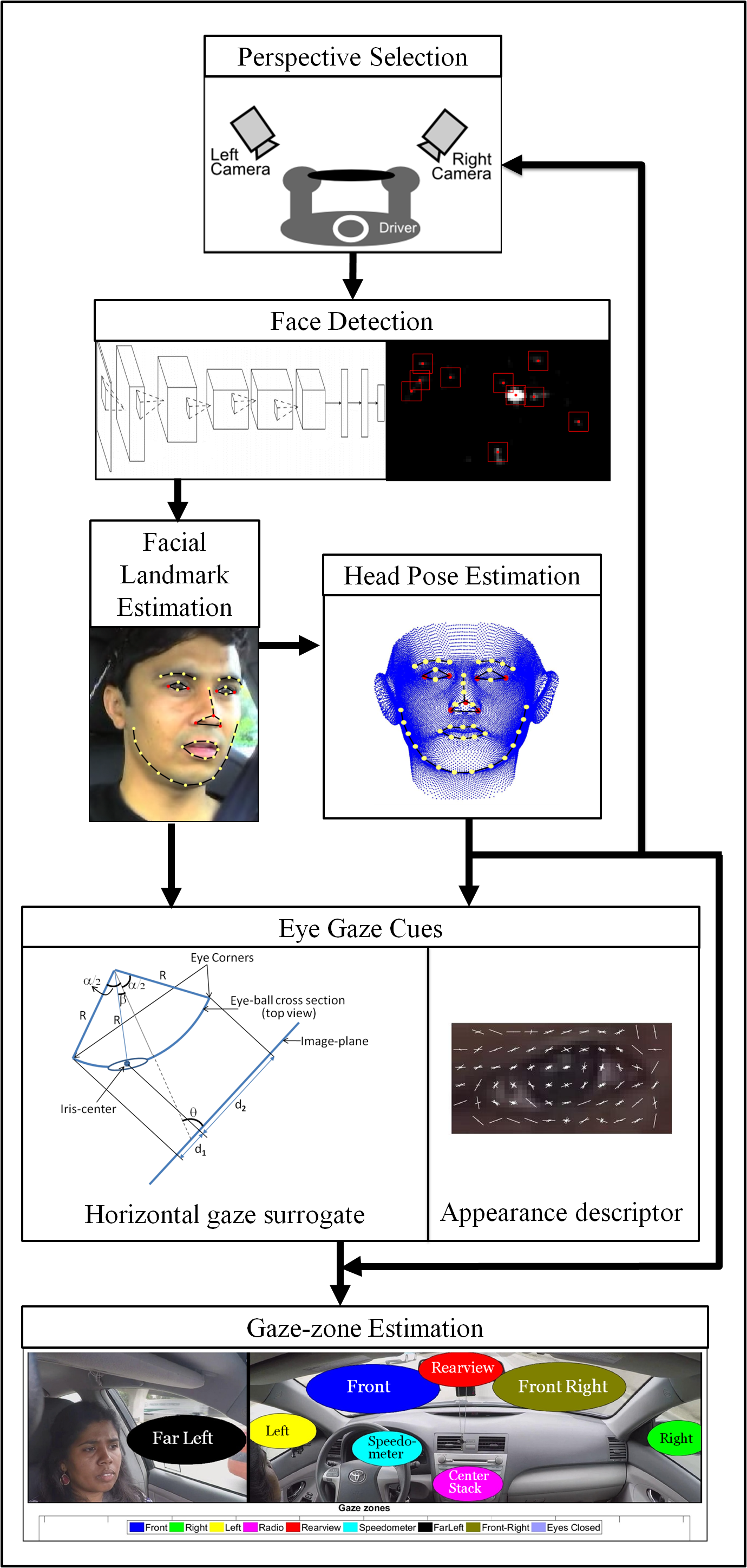
Figure 2: A illustrative block diagram showing the process of estimating gaze zone from time of capture from multiple camera perspectives to classifying gaze into one of nine gaze zones (i.e. eight gaze zones illustrated above and “eyes closed”). Key modules in the system include deep CNN based face detection [22], landmark estimation [23], horizontal gaze surrogate [11], appearance descriptor and head pose based perspective selector [21].

• Facial landmark estimation: The landmarks are estimated using a cascade of regression models as described in [24, 23] with more details for iris localization given in [11].

• Head pose estimation: A geometric method where local features, such as eye corners, nose corners, and the nose tip, and their relative 3-D configurations, determine the pose [21].

• Horizontal gaze surrogate: The horizontal gaze-direction $\beta$ with respect to head, see Figure 2, is estimated as a function of $\alpha$, angle subtended by an eye in horizontal direction, head-pose (yaw) angle $\theta$ with respect to the image plane, and $\frac{d_{1}}{d_{2}}$, the ratio of the distances of iris center from the detected corner of the eyes in the image plane [11].

• Appearance descriptor: Appearance of the eye is represented by computing HoG (Histogram of Gradients) [25] in a 2-by-2 patch around the eye. This descriptor is especially designed to capture the vertical gaze of the eyes.

• Gaze zone estimation: Eight semantic gaze-zones of interest are, far left, left, front, speedometer, rear view, center stack, front right and right, as illustrated in Figure 2. Another class of interest, but not illustrated in the figure, is the state of eyes closed. Consider a set of feature vectors $\vec{F}=\{\vec{f}_{1},\vec{f}_{2},\dots,\vec{f}_{N}\}$, and their corresponding class labels $X=\{x_{1},x_{2},\dots,x_{N}\}$, for $N$ sample instances. Here a feature vector is a concatenation of head pose and eye cues described above and class labels are one of nine gaze zones. Given $\vec{F}$ and $X$, a random forest (RF) is trained on the corpus.

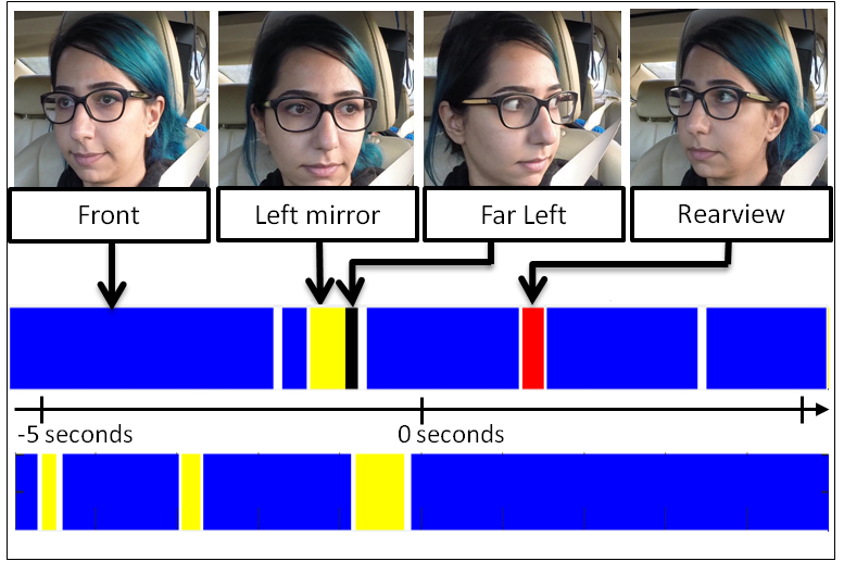
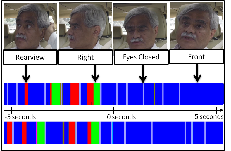
(a) Two Left Lane Change Events	(b) Two Right Lane Change Events

Figure 3: Illustrates four different scanpaths during a 10-second time window prior to lane change, two scanpaths during left lane change and two scanpaths during right lane change event, with sample face images from various gaze zones. Consistencies such as total glance duration and number of glances to regions of interest within a time window are useful to note when describing the nature of driver’s gaze behavior. Such consistencies can be used as features to predict behaviors. See Figure 2 for a legend of which color is associate with which gaze zone.

III-B Spatio-Temporal Feature Descriptor

The gaze estimator, as described in the previous section, outputs where the driver is looking in a given instance. A continuous segment of gaze estimates of where the driver has been looking is referred to as a scanpath. Figure 3 illustrates multiple scanpaths in a 10-second time window around lane change, two scanpaths from left lane change and two scanpaths from right lane change events. In the figure, the x-axis represents time and the color displayed at a given time $t$ represents the estimated gaze zone. Let SyncF denote the time when the tire touches the lane marking before crossing into the next lane, which is the ”0-seconds” displayed in the figure. Visually, in the 5-second time period before SyncF, there is some consistency observed across the different scanpaths within a given event (e.g. left lane change); consistencies such as the minimum glance duration in relevant gaze zones. For example, in the scanpaths associated with right lane change, the driver glances at the rearview and right gaze zones for a significant duration. However, the start and end point of the glances are not necessarily the same across the different scanpaths. Therefore, we represent the scanpaths using features called gaze accumulation, glance frequency and glance duration, which remove some temporal dependencies but still capture sufficient spatio-temporal information to distinguish between different gaze behaviors.

As these features are computed over a time window, we, first, define signals necessary to compute them. Let $Z$ represent the set of all nine gaze zones as $Z=$ {Front, Right, Left, Center Stack, Rearview, Speedometer, Left Shoulder, Right Windshield, Eyes Closed} and let $L=|Z|$ represent the total number of gaze zones. Let the vector $G=[g_{1},g_{2},\dots,g_{N}]$ represent the estimated gaze for an arbitrary time period of $T$, where $N=\textit{fps(frames per second)}\times T$, $g_{n}\in Z$, and $n\in\{1,2,\dots,N\}$. The following description defines how to compute gaze accumulation, glance duration and glance frequencies given $G$.

III-B1 Gaze Accumulation

Gaze accumulation is a vector of size $L$, where each entry is a function of a unique gaze zone. Given a gaze zone, gaze accumulation is the accumulated sum of the number of times driver looked at the zone of interest within a time period; which is then normalized by the time window for relative accumulation. Mathematically, gaze accumulation at gaze zone $z_{j}$, where $j\in\{1,2,...,L\}$ corresponds to the $j^{th}$ gaze zone in $Z$, is as follows:

$$\textit{Gaze Accumulation }(z_{j})=\frac{1}{N}\times\sum_{n=1}^{N}\mathbbm{1}(g_{n}==z_{j})$$

where $\mathbbm{1}(\bullet)$ is the indicator function.

III-B2 Glance frequency

Glance frequency is a vector of size $L$, where each entry is a function of a unique gaze zone. Within time period $T$, every time there is a transition from one gaze zone to another (e.g. Front to Speedometer), the glance count for the destination gaze zone is incremented; the count is then normalized by the time period to produce glance frequency. Under the condition that estimates are noise free, glance frequency for each of the gaze zones, $z_{j}$, where $j\in\{1,2,...,L\}$ corresponds to the $j^{th}$ gaze zone in $Z$, is calculated as follows:

Glance $$\textit{Frequency }(z_{j})$$

$$=\frac{1}{T}\times\sum_{n=2}^{N}\mathbbm{1}(g_{n}==z_{j})\times\mathbbm{1}(g_{n-1}\neq z_{j})$$

However, since gaze estimates are noisy, a majority rule over a buffered window is necessary to acknowledge transition into a new gaze zone. Algorithm 1 details calculation of the glance frequency while accounting for noisy estimation.

III-B3 Glance Duration

Glance duration is a vector of size $L$, where each entry is a function of a unique gaze zone. Given a gaze zone, glance duration is the longest glance made towards the gaze zone of interest within time window $N$. Following the same process as in Algorithm 1, in addition to counting when transitions to new gaze zones occur, the start and end of each continuous glance can also be tracked. For gaze zone $z_{j}$, let $S_{z_{j}}$ be a $[N_{j}\times 2]$-matrix indicating the start and end index of $N_{j}=\textbf{C}_{G}(z_{j})$ continuous glance, where $\textbf{C}_{G}(z_{j})$ is the number of continuous glances to $z_{j}$ as computed in Algorithm 1. Glance duration for each of the gaze zones, $z_{j}$, where $j\in\{1,2,...,L\}$ corresponds to the $j^{th}$ gaze zone in $Z$, is calculated as follows:

$$\textit{Glance Duration }(z_{j})=\begin{cases}\max\limits_{1\leq n\leq N_{j}}\left|\delta(S_{z_{j}}(n,:)\right|&\textit{if }N_{j}>0\\ 0&\textit{if }N_{j}=0\end{cases}$$

where $\delta(\bullet)$ is the difference operator.

The final feature vector, $\vec{h}$, representing a scanpath then is made up of a combination of the above described descriptors. In particular, this paper will explore the benefits of representing a scanpath in three different ways: gaze accumulation alone, glance duration alone and glance duration plus glance frequency.

III-C Gaze Behavior Modeling

Consider a set of feature vectors $\vec{H}=\{\vec{h}_{1},\vec{h}_{2},\dots,\vec{h}_{N}\}$, and their corresponding class labels $Y=\{y_{1},y_{2},\dots,y_{N}\}$. In this paper, the class labels will be maneuvers: Left Lane Change, Right Lane Change, Lane Keeping. The gaze behaviors of respective events, tasks or maneuvers, are then modeled using an unnormalized multivariate normal distribution (MVN):

$$M_{b}(\vec{h})=\exp\left(-\frac{1}{2}(\vec{h}-\vec{\mu_{b}})^{T}\Sigma_{b}^{-1}(\vec{h}-\vec{\mu_{b}})\right)$$

where $b\in B=$ {Left Lane Change, Right Lane Change, Lane Keeping}, and $\mu_{b}$ and $\Sigma_{b}$ represent mean and covariance computed over the training feature vectors for the gaze behavior represented by $b$. One of the reasons for modeling gaze behavior in such a way is, given a new test scanpath descriptor, $\vec{h}_{test}$, we want to know how does it compare to the average scanpath computed for each gaze behavior in the training corpus. One possibility is to compute the euclidean distance between the average scanpath descriptor, $\mu_{b}$, and the test scanpath descriptor, $\vec{h}_{test}$, for all $b\in B$, and assign the label with the shortest distance. However, this assigns equal weight or penalty to every component in $\vec{h}$. The weights, however, should be a function of component as well as behavior under consideration. Therefore, we use the Mahalanobis distance, which assigns weights appropriately based on expected variance in the training data. Furthermore, by exponentiating the Mahalanobis distance to produce the unnormalized MVN, the range is mapped between $0$ and $1$. To a degree this can be used to asses the probability or confidence that a certain test scanpath represented by its descriptor, $\vec{h}_{test}$, belongs to a particular gaze behavior model.

input : $G=[g_{1},g_{2},\dots,g_{N}]$ are noisy gaze estimates
$W$, a positive time window threshold for consistency check, $<N$

output : A vector, $\textit{{F}}_{G}$, of frequency of glances

LastGazeState$=g_{1}$

for $i\leftarrow W$ to $N$ do

       if $g_{i}\neq\textit{LastGazeState}$ then

             if Majority ($g_{i}==[g_{i-1}\cdots g_{i-W}])$ then

                   $\textbf{C}_{G}(g_{i})++$;

                   $\textit{LastGazeState}=g_{i};$

             end if

            

       end if

      i++;

end for

$\textbf{F}_{G}=\frac{1}{T}\times\textbf{C}_{G};$

Algorithm 1 To compute a vector of glance frequencies given noisy estimates of gaze zones over time period $T$ with $N$ frames.

IV Experimental Design and Analysis

IV-A Naturalistic Driving Dataset

A large corpus of naturalistic driving dataset is collected using an instrumented vehicle testbed. The vehicular tested is instrumented to synchronously capture data from camera sensors for looking-in and looking-out, radars, LIDARs, GPS and CAN bus. Of interest in this study are two camera sensors looking at the driver (i.e. one near the rearview mirror and another near the A-pillar) and one camera sensor looking-out in the driving direction. As the focus of this study is in driver gaze dynamics, the looking out view is only used to provide context for data mining. Using the same instrumented vehicle test, seven drivers of varying driving experience drove the car on different routes for an average of 40 minutes (see Table I). Each drive consisted of some parts in urban settings, but mostly in freeway settings with multiple lanes. As the drivers are familiar with the area and were given the independence to design their own routes, the dataset contains natural glance behavior during driving maneuvers.

Table I: Description of analyzed on-road driving data.

	Duration	No. of Events
Driver	Full drive	Left Lane	Right Lane	Lane
ID	[min]	Change	Change	Keeping
1	52.10	9	5	20
2	24.25	5	5	60
3	28.13	5	4	50
4	36.38	10	4	32
5	39.20	10	4	45
6	27.49	6	5	80
7	37.50	5	5	46
All	273.30	50	32	333

From the collected dataset of seven drivers, several types of annotations were done

• Gaze zone annotation of approximately equal number of samples with respect to the gaze-zones for all seven drivers. Each sample was annotated only when the annotator was highly confident that without ambiguity the sample falls into one of nine gaze-zone classes. Some annotated samples are from consecutive video frames while others are not. For a full description, the readers are referred to [26]. Let’s call this the Gaze-zone-dataset.

• Left and right lane change event annotations for all drivers. As a point of synchronization, for lane change events, when the vehicle tire is about to cross over into the other lane, it is marked at annotation and denoted as SyncF. A 20-second window centered on SyncF, makes up the event. At the time of training and testing, however, gaze dynamics is computed on a sliding 5-second window (see Section IV-C). Accumulated number of these events per driver and overall are given in Table I. Let’s call this the Lane-change-events-dataset.

• Lane keeping event annotations for all drivers. Lengthy stretches of lane keeping (as seen from looking-out camera) are broken into non-overlapping 5-second time window segments to create lane keeping events. Table I contains the number of such events annotated and considered for the following analysis. Let’s call this the Lane-keeping-events-dataset.

• Gaze zone annotation of every frame in the Lane-change-events-dataset. When annotating each of the 20-second continuous video segment, human annotators had to make a choice between one of the nine zones or unknown. When ambiguous samples arose, the annotators used temporal information and outside context to make the call. Unknown was highly discouraged to be used except for transitions between zones. Let’s call this the Gaze-dynamics-dataset.

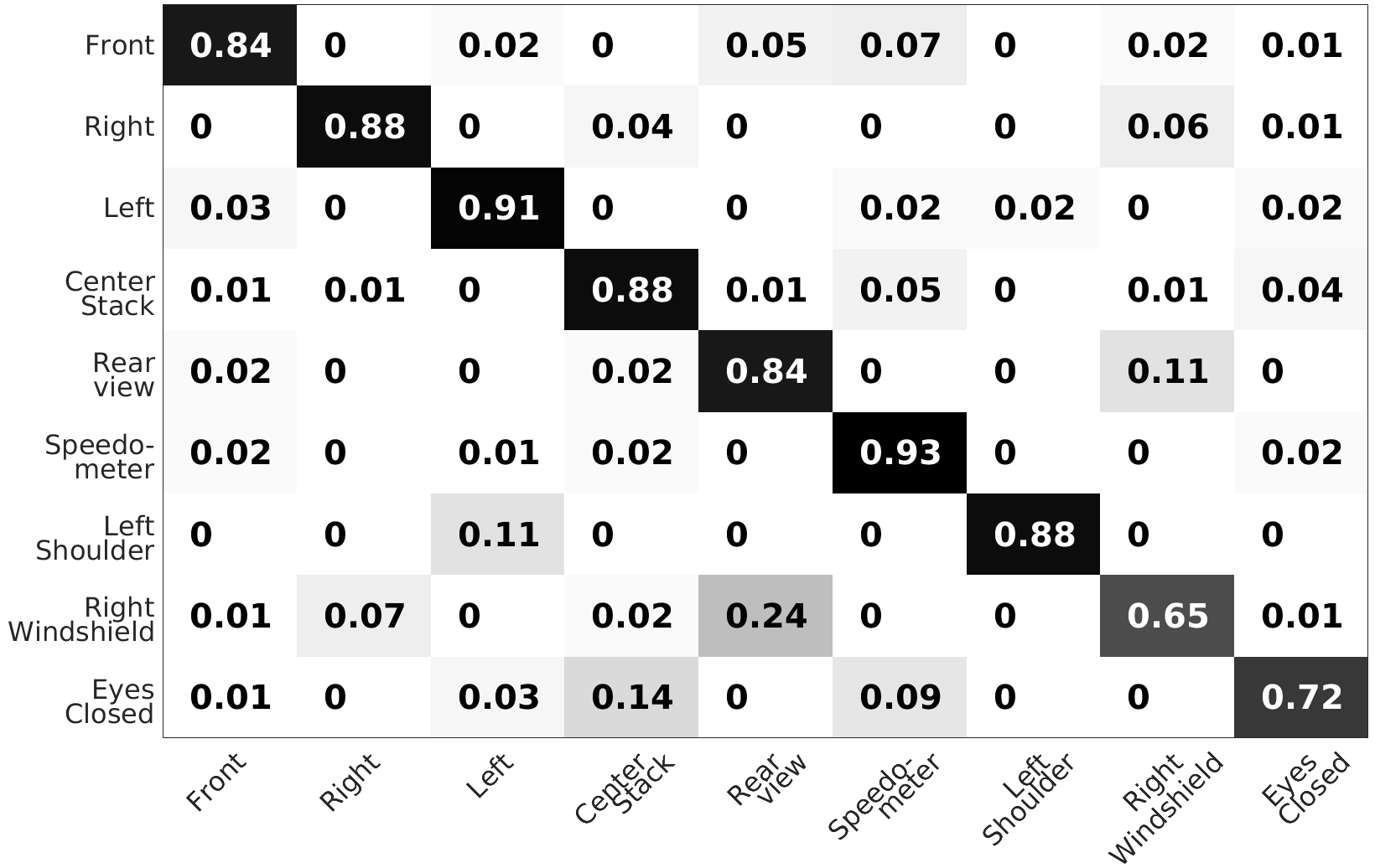
Figure 4: Evaluation of our gaze estimator on Gaze-zone-datase which is comprised of balanced samples with respect to gaze zones for each of the seven drivers. The confusion matrix is generated from a leave one driver out cross-validation, where the rows are true classes and columns are estimates. The rows as displayed may not sum to one because of Unknown-class.

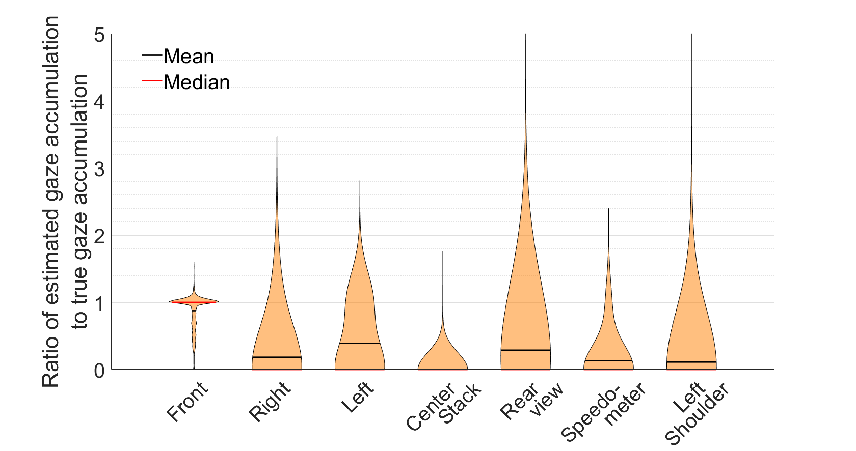
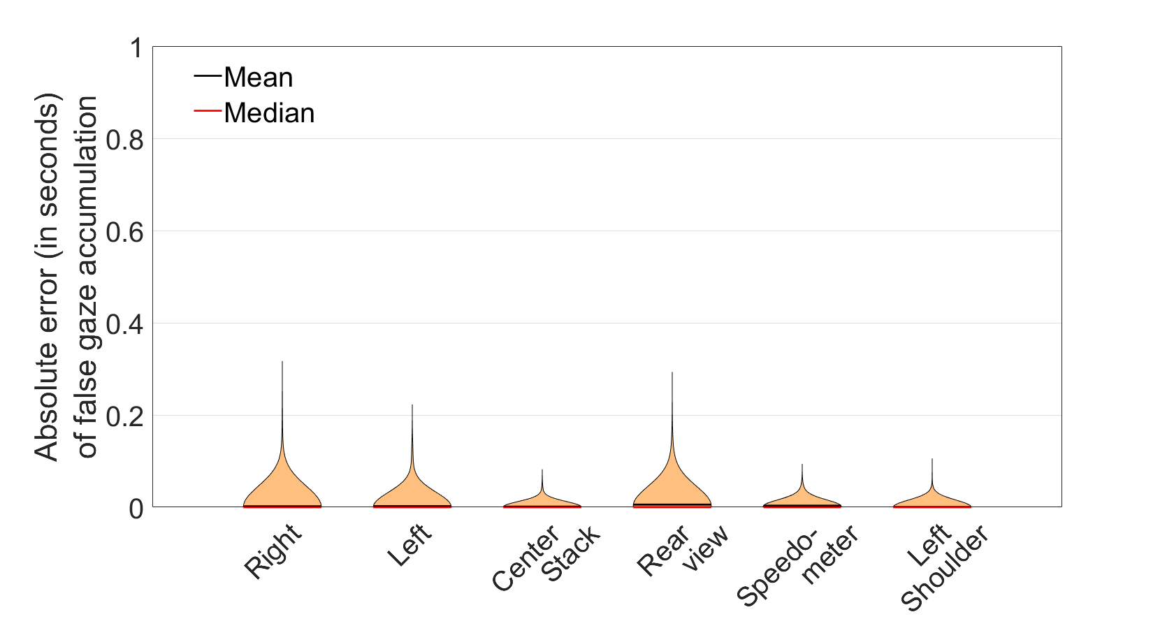
(a) Gaze accumulation ratio of true positives	(b) Gaze accumulation error of false positives

Figure 5: Performance evaluation of the gaze zone estimator is presented as a violin plot, which is a relative distribution of applying the following two metrics to all the samples in the Gaze-dynamics-dataset: (a) ratio of estimated to true gaze accumulation (Eq. 1) and (b) absolute error in estimated gaze accumulation due to false positives (Eq. 2). The width of the violin at respective values of the y-axis dictates the relative likelihood of the value for the gaze zone in the x-axis. Ideally, the width is largest for the ratio metric around one and for the absolute error metric around zero, meaning when true positives occur the durations of the estimated glances is close to durations of the true glances and when false positives occur the durations of those estimated glances are negligibly small.

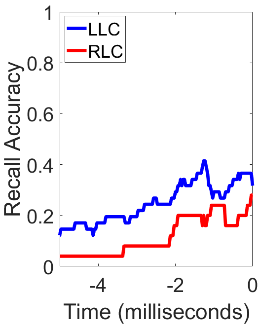
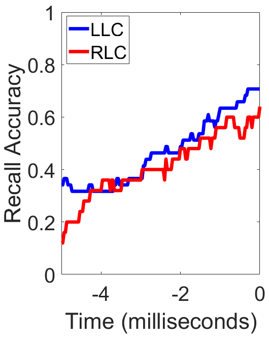
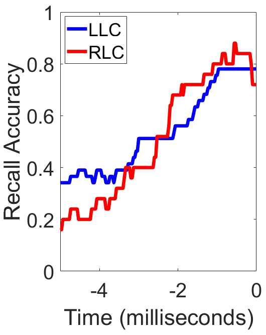
(a) Glance Duration + Frequency	(b) Glance Duration only	(c) Gaze accumulation

Figure 6: The recall accuracy of lane change prediction (averaged and cross-validated across all drivers in the naturalistic driving scenarios) continuously from -5 seconds to 0 seconds prior to lane change for three different combinations of spatio-temporal feature descriptors: (a) glance duration plus glance frequency, (b) glance duration only and (c) gaze accumulation only. LLC stands for left lane change and RLC stands for right lane change

IV-B Evaluation of Gaze Dynamics

Of the literary works listed in Table LABEL:table:relatedWorks which estimate gaze automatically, many of them output one of a number of gaze zones of interest. In those works, performance evaluation of their gaze estimator is presented in terms of a confusion matrix on what percent are correctly classified and what percent are misclassified with respect to the gaze zones. The advantage of such a presentation of evaluation is that when gaze zones are classified incorrectly, it shows what it is misclassified into and more often than not, the misclassification occurs in spatially neighboring zones (e.g. Front and Speedometer). As for the dataset over which evaluation occurs, no guarantee is given that consecutive frames are annotated; in fact in [11], annotations were done every 5 frames. As a point of comparison, Figure 4 presents results of our gaze estimator (as described in Section III-A) on the Gaze-zone-dataset as a confusion matrix with a weighted accuracy of 83.5% (i.e. accuracy is calculated per gaze zone and averaged over all gaze zones) from leave one driver out cross-validation.

There are two important and often overlooked facts about this form of evaluation when considering the application of the gaze estimator on continuous video sequences and the interest is on semantics like gaze accumulation, glance durations and glance frequencies. First is the lack of evaluation on images or video frames where driver’s gaze is in transition between two gaze zones. Since the gaze estimator is not explicitly trained to classify transition states, the gaze estimator is expected to ideally classify those transition instances into one of the two gaze zones that it is in transition between. Second is the lack of metrics to garner the effects of misclassification error on a continuous segment. For instance, consider the highest misclassification rate between front right windshield and rearview mirror seen in the confusion matrix in Figure 4. When does the misclassification occur? In the periphery of a continuous glance, in the middle of a glance or in transition between glances? Depending on the type of misclassification, it will affect glance duration and frequency calculation.

The first limitation is addressed by creating the Gaze-dynamics-dataset. To address the latter limitation, this paper introduces two performance evaluation metrics for gaze dynamics with respect to gaze accumulation. One is the ratio of estimated gaze accumulation to true gaze accumulation per gaze zone:

$$\textit{Relative ratio of $\hat{A}_{G}$ }(z_{j})=\begin{cases}\frac{\hat{A}_{G}(z_{j})}{A_{G}(z_{j})}&\textit{if }A_{G}(z_{j})\neq 0\\ 0&\textit{if }A_{G}(z_{j})=0\par\end{cases}$$ (1)

where $A_{G}(z_{j})$ is the gaze accumulation calculated from ground truth annotation of gaze zones over a time period for gaze zone $z_{j}$ and $\hat{A}_{G}(z_{j})$ is the gaze accumulation calculated from estimated gaze zones over a time period for gaze zone $z_{j}$. Note that in a given time window, only true positive gaze zone accumulation is considered with the first metric. Therefore, the second metric is designed to account for false gaze accumulations:

$$\textit{Abs error of $\hat{A}_{G}$ }(z_{j})=\begin{cases}0&\textit{if }A_{G}(z_{j})\neq 0\\ \hat{A}_{G}(z_{j})&\textit{if }A_{G}(z_{j})=0\par\end{cases}$$ (2)

These new performance metrics are applied to the Gaze-dynamics-dataset, where each of the 20-second videos are broken into 5-second segments with up to 4-second overlaps resulting in a total of 1312 samples. The performance is illustrated using a violin plot in Figure 5; a violin plot is a distribution of the output of the metrics over all the samples in respective gaze zone classes. Ideally, the ratio metric (Eq. 1) is concentrated around 1, however, as seen in Figure 5, only the front gaze zone follows such a pattern. This result shows promise of accurately detecting attention versus inattention to the forward driving direction because the ratio of estimated to true gaze accumulation is highly concentrated around 1 for Front gaze zone. Meanwhile, for other gaze zones, in majority of the samples, estimated gaze accumulation is less than the true gaze accumulation; this is mainly because glances towards these regions are significantly shorter in duration when compared to glance towards Front and therefore more prone to noisy estimates.

The second metric (Eq. 2) tries to answer the following questions: what happens when given a time period, ground truth annotations do not contain any annotations of a particular gaze zone but the gaze estimator produces false positives? Are the false positives sparse or significant in time? According to Figure 5b, the false gaze accumulations are small relative to the 5-second window over which the gaze accumulation is calculated. Ideally, when calculating gaze accumulation over a time segment of estimated gaze zones, the ratio metric (Eq. 1) should be around one and the absolute error metric (Eq. 2) should be around zero, meaning when true positives occur the durations of the estimated glances is close to durations of the true glances and when false positives occur the durations of those falsely estimated glances are negligibly small.

IV-C Evaluation on Gaze Modeling

All evaluations conducted in this study is done with a seven-fold cross validation; seven because there are seven different drivers as outlined in Table I. With this setup of separating the training and testing samples, we explore the recall accuracy of the gaze behavior model in predicting lane changes as a function of time (Figure 6).

Training occurs on the 5-second time window before SyncF as represented by the events in Table I. Note that, manually annotated gaze zones are used to compute the spatio-temporal features used to train the lane change models whereas estimated gaze zones are used to train the lane keeping model. In testing, however, only estimated gaze-zones are used to compute spatio-temporal features.

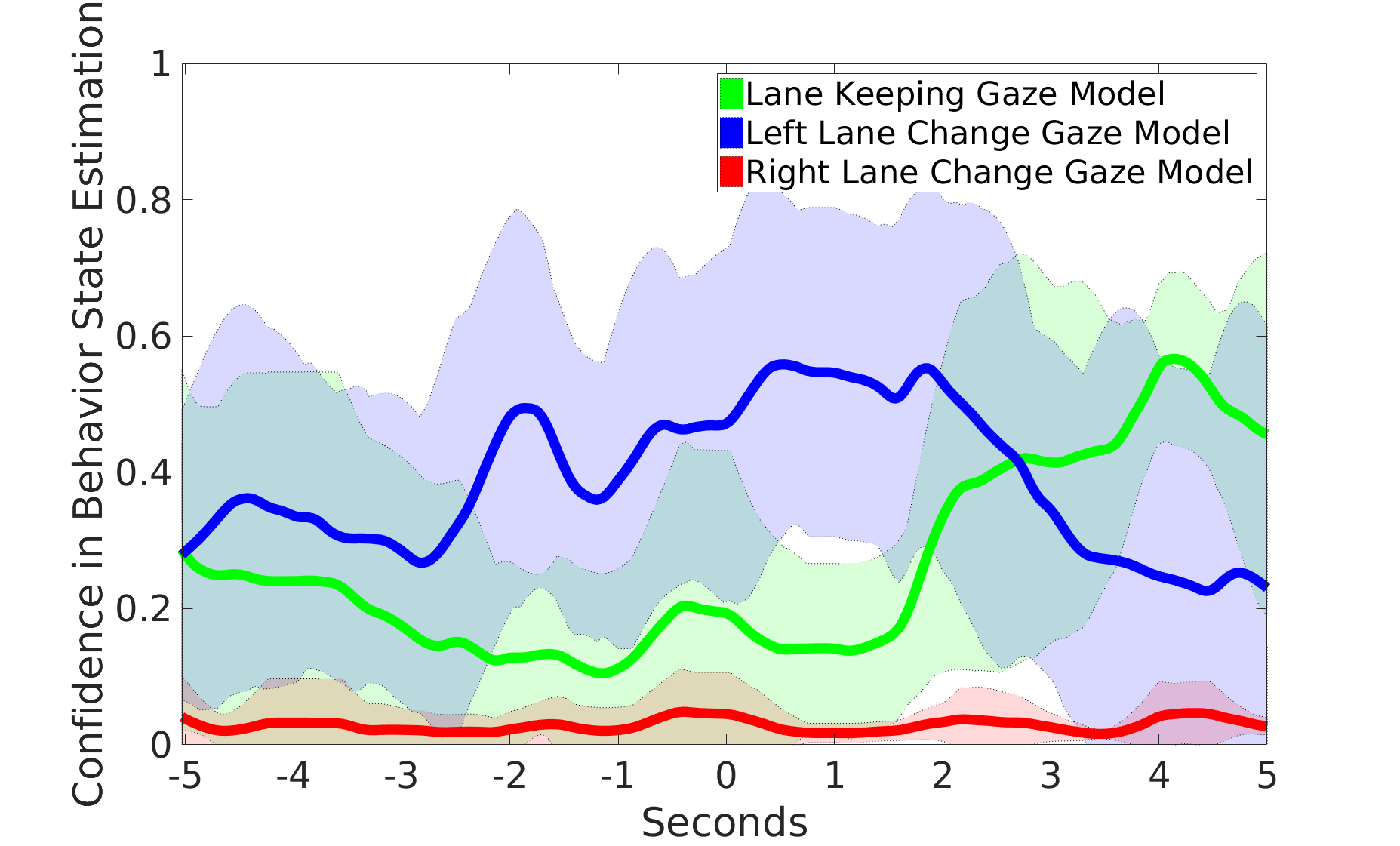
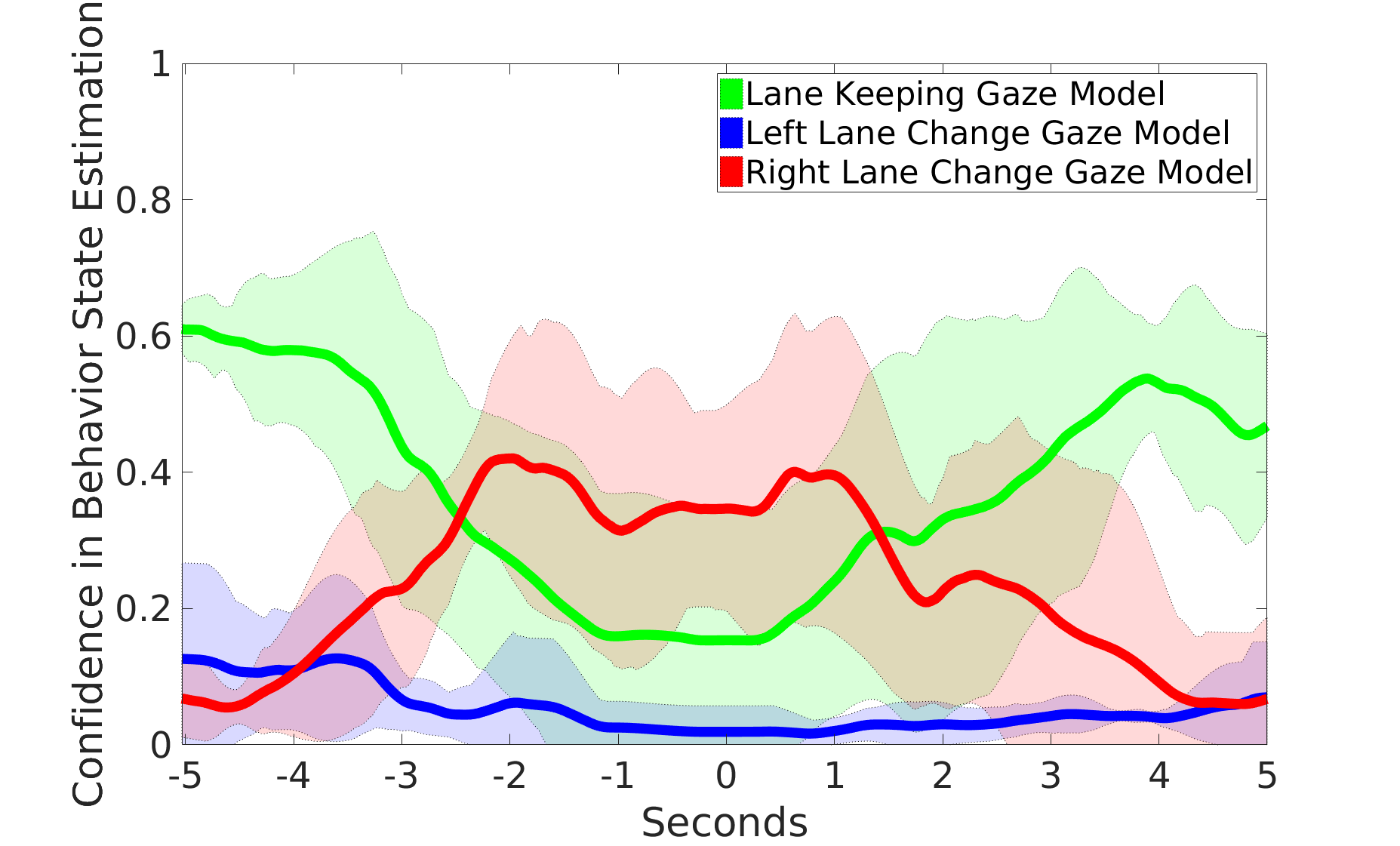
(a) Left Lane Change Events (DriverID 2)	(b) Right Lane Change events (DriverID 2)
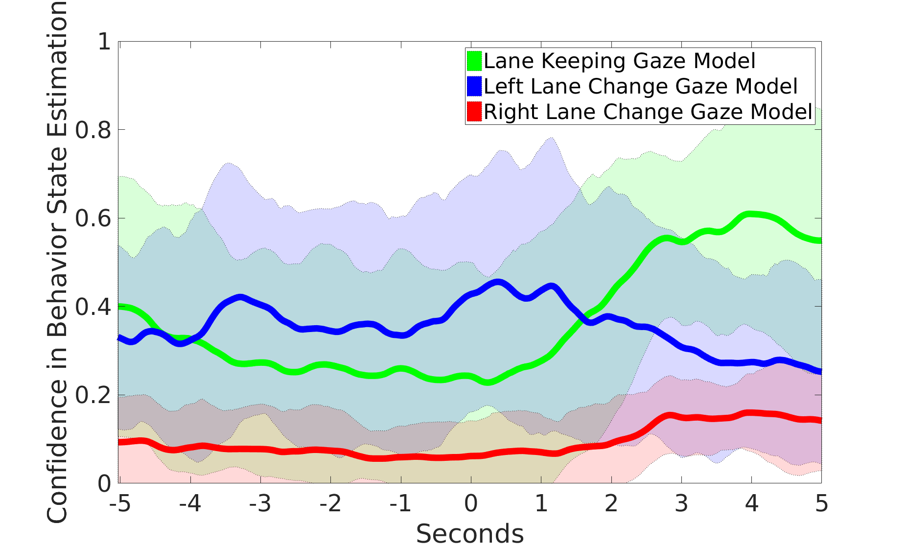
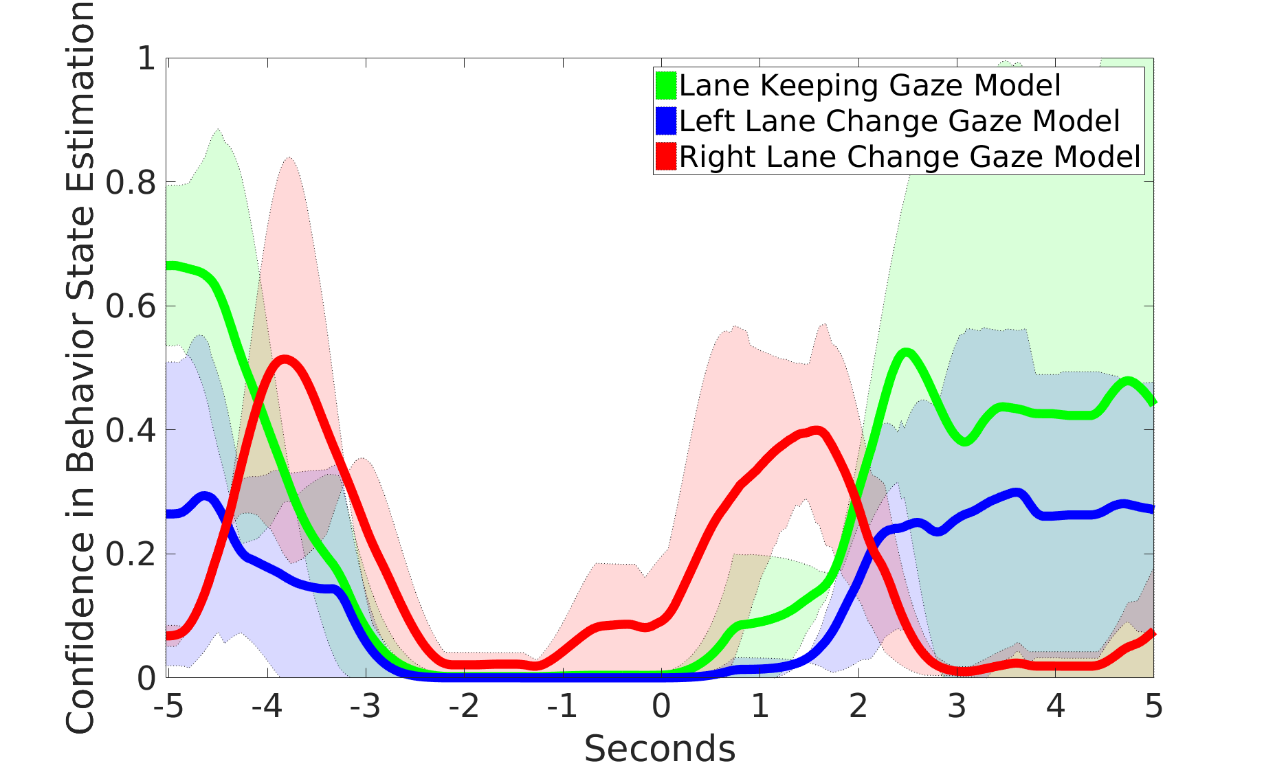
(c) Left Lane Change Events (Driver ID 5)	(d) Right Lane Change events (DriverID 5)

Figure 7: Illustrates variations in fitness of the three models (i.e. Left lane change, Right lane) during left and right lane change maneuvers for two different drivers, where mean and standard deviation are depicted with solid line and semitransparent shades, respectively.

At testing time, we want to test how early the gaze behavior models are able to predict lane change. Therefore, starting from 5-seconds before SyncF sequential samples with $\frac{1}{30}$ of a second overlap are extracted up to 5-seconds after SyncF; note that the time window at 5-seconds before the SyncF encompasses data from 10 seconds before the SyncF up to 5-seconds before the SyncF. Each of the samples are tested for fitness across the three gaze behavior models, namely models for left lane change, right lane change and lane keeping. The sample is assigned the label based on the model which procures the highest fitness score and if the label matches the true label the sample is considered a true positive. Note that each test sample is associated with a time index of where it is sampled from with respect to SyncF. By gathering samples at the same time index with respect to SyncF, recall value at a given time index is calculated by dividing the number of true positives by the total number of positive samples.

When calculating recall values, true labels of samples were remapped from three classes to two classes; for instance, when computing recall values for left lane change prediction, all right lane change events and lane keeping events were considered negatives samples and only the left lane change events are considered positive samples. Similar procedure is observed for computing recall values for right lane change prediction. Figure 6 shows the development of the recall values for both left and right lane change prediction continuously from -5 seconds prior to SyncF up to 0 milliseconds prior to SyncF for three different combinations of features (i.e. glance duration plus frequency, glance duration only and gaze accumulation only) and for two events (i.e. left lane change and right lane change). As expected the recall curves rise in accuracy the closer in time to the lane change event. Also expected is the performance difference with respect to the spatio-temporal features; whereas modeling with gaze accumulation alone achieves above 75% accuracy at 1000 milisecond prior to lane change, modeling with glance duration alone and glance duration plus frequency achieves about 60% and 40% accuracy, respectively. One possible reason for the stark difference in performance when using gaze accumulation versus glance duration and frequency is the latter may vary across drivers more than the former. For example, one driver may exhibit short glances with high frequency whereas another driver may make long glances with low frequency. However, gaze accumulation neatly maps the differences in gaze behavior to one “attention” allocation domain and therefore gives the best performance under given modeling methods and dataset.

Lastly, in Figure 7, we illustrate the fitness or confidence of the learned models around left and right lane change maneuvers for two different drivers. The figure shows mean (solid line) and standard deviation (semitransparent shades) of three models (i.e. left lane change, right lane change, lane keeping) using the events from naturalistic driving dataset described in Table I. The model confidence statistics are plotted 5 seconds before and after the lane change maneuver, where time of 0 seconds represents when the vehicle is about to change lanes. Interestingly, even though early versus late peaks of the appropriate model can be uniquely different across drivers and maneuvers, the satisfactory separation of the lane change models to lane keeping model and the spread in dominance of the correct model shows promise in modeling driver behavior using gaze dynamics to anticipate activities and maneuvers.

V Concluding Remarks

In this study, we explored modeling driver’s gaze behavior in order to predict maneuvers performed by drivers, namely left lane change, right lane change and lane keeping. The particular model developed in this study features three major aspects: one is the spatio-temporal features to represent the gaze dynamics, second is in defining the model as the average of the observed instances, third is in the design of the metric for estimating fitness of model. Applying this framework in a sequential series of time windows around lane change maneuvers, the gaze models were able to predict left and right lane change maneuver with an accuracy above 75% around 1000 milliseconds before the maneuver.

The overall framework, however, is designed to model driver’s gaze behavior for any tasks or maneuvers performed by driver. In particular, the spatio-temporal feature descriptor composed of gaze accumulation, glance duration and glance frequency are powerful tools to capture the essence of recurring driver gaze dynamics. To this end, there are multiple future directions in site. One is to quantitatively define the relationship between the time window from which to extract those meaningful spatio-temporal features and the task or maneuvers performed by driver. Other future directions are in exploring and comparing different temporal modeling approaches and generative versus discriminative models.

Sujitha Martin received the BS degree in Electrical Engineering from the California Institute of Technology in 2010 and the MS and Ph.D degree in electrical engineering from the University of California, San Diego (UCSD) in 2012 and 2016, respectively. She is currently a research scientist at Honda Research Institute USA. Her research interests are in machine vision and learning, with a focus on human-centered, collaborative, intelligent systems and environments. She helped organize two workshops on analyzing faces at the IEEE Intelligent Vehicles Symposium (IVS 2015, 2016) and the first Women in Intelligent Transportation Systems (WiTS) meet and greet networking event at the IEEE IVS (2017). She is recognized as one of top female graduates in the fields of electrical and computer engineering and computer science at Rising Stars 2016 hosted by Carnegie Mellon University.

Sourabh Vora received his BS degree in Electronics and Communications Engineering (ECE) from Birla Institute of Technology and Science (BITS) Pilani - Hyderabad Campus. He received his MS degree in Electrical and Computer Engineering (ECE) from University of California, San Diego (UCSD) where he was associated with the Computer Vision and Robotics Research (CVRR) Lab. His research interests lie in the field of Computer Vision and Machine Learning. He is currently working as a Computer Vision Engineer at nuTonomy, Santa Monica.

Kevan Yuen Kevan Yuen received the B.S. and M.S. degrees in electrical and computer engineering from the University of California, San Diego, La Jolla. During his graduate studies, he was with the Computer Vision and Robotics Research Laboratory, University of California, San Diego. He is currently pursuing a PhD in the field of advanced driver assistance systems with deep learning, in the Laboratory of Intelligent and Safe Automobiles at UCSD.

Mohan Manubhai Trivedi is a Distinguished Professor of and the founding director of the UCSD LISA: Laboratory for Intelligent and Safe Automobiles, winner of the IEEE ITSS Lead Institution Award (2015). Currently, Trivedi and his team are pursuing research in distributed video arrays, human-centered self-driving vehicles, human-robot interactivity, machine vision, sensor fusion, and active learning. Trivedi’s team has played key roles in several major research initiatives. Some of the professional awards received by him include the IEEE ITS Society’s highest honor “Outstanding Research Award” in 2013, Pioneer Award (Technical Activities) and Meritorious Service Award by the IEEE Computer Society, and Distinguished Alumni Award by the Utah State University and BITS, Pilani. Three of his students were awarded “Best Dissertation Awards” by professional societies and 20+ “Best” or “Honorable Mention” awards at international conferences. Trivedi is a Fellow of the IEEE, IAPR and SPIE. Trivedi regularly serves as a consultant to industry and government agencies in the U.S., Europe, and Asia.

References

- [1] M. M. Trivedi, T. Gandhi, and J. McCall, “Looking-in and looking-out of a vehicle: Computer-vision-based enhanced vehicle safety,” Intelligent Transportation Systems, IEEE Transactions on, 2007.
- [2] A. Doshi and M. M. Trivedi, “Tactical driver behavior prediction and intent inference: A review,” in Conference on Intelligent Transportation Systems. IEEE, 2011.
- [3] J. S. International, “Taxonomy and definitions for terms related to on-road motor vehicle autmated driving systems,” 2014.
- [4] S. M. Casner, E. L. Hutchins, and D. Norman, “The challenges of partially automated driving,” Communications of the ACM, 2016.
- [5] A. Jain, H. S. Koppula, B. Raghavan, S. Soh, and A. Saxena, “Car that knows before you do: Anticipating maneuvers via learning temporal driving models,” ICCV, 2015.
- [6] C. Gold, D. Damböck, L. Lorenz, and K. Bengler, ““take over!” how long does it take to get the driver back into the loop?” in Proceedings of the Human Factors and Ergonomics Society Annual Meeting. SAGE Publications, 2013.
- [7] A. Tawari and B. Kang, “A computational framework for driver’s visual attention using a fully convolutional architecture,” in Intelligent Vehicles Symposium (IV). IEEE, 2017.
- [8] A. Palazzi, F. Solera, S. Calderara, S. Alletto, and R. Cucchiara, “Learning where to attend like a human driver,” in Intelligent Vehicles Symposium (IV). IEEE, 2017.
- [9] F. Vicente, Z. Huang, X. Xiong, F. De la Torre, W. Zhang, and D. Levi, “Driver gaze tracking and eyes off the road detection system.” IEEE.
- [10] X. Zhang, Y. Sugano, M. Fritz, and A. Bulling, “It’s written all over your face: Full-face appearance-based gaze estimation,” in IEEE Conference on Computer Vision and Pattern Recognition Workshops, 2017.
- [11] A. Tawari, K. H. Chen, and M. M. Trivedi, “Where is the driver looking: Analysis of head, eye and iris for robust gaze zone estimation,” in Conference on Intelligent Transportation Systems (ITSC). IEEE, 2014.
- [12] A. Tawari, A. Møgelmose, S. Martin, T. B. Moeslund, and M. M. Trivedi, “Attention estimation by simultaneous analysis of viewer and view,” in 17th International IEEE Conference on Intelligent Transportation Systems (ITSC). IEEE, 2014.
- [13] S. Martin and M. M. Trivedi, “Gaze fixations and dynamics for behavior modeling and prediction of on-road driving maneuvers,” in Intelligent Vehicles Symposium Proceedings, 2017.
- [14] C. Ahlstrom, K. Kircher, and A. Kircher, “A gaze-based driver distraction warning system and its effect on visual behavior,” Intelligent Transportation Systems, IEEE Transactions on, 2013.
- [15] L. Fridman, J. Lee, B. Reimer, and T. Victor, “Owl and lizard: Patterns of head pose and eye pose in driver gaze classification,” IET Computer Vision, 2016, In Print.
- [16] S. A. Birrell and M. Fowkes, “Glance behaviours when using an in-vehicle smart driving aid: A real-world, on-road driving study,” Transportation research part F: traffic psychology and behaviour, 2014.
- [17] M. Muñoz, B. Reimer, J. Lee, B. Mehler, and L. Fridman, “Distinguishing patterns in drivers’ visual attention allocation using hidden markov models,” Transportation research part F: traffic psychology and behaviour, 2016.
- [18] N. Li and C. Busso, “Detecting drivers’ mirror-checking actions and its application to maneuver and secondary task recognition,” IEEE Transactions on Intelligent Transportation Systems, 2016.
- [19] L. Fridman, H. Toyoda, S. Seaman, B. Seppelt, L. Angell, J. Lee, B. Mehler, and B. Reimer, “What can be predicted from six seconds of driver glances?” 2017.
- [20] B. Vasli, S. Martin, and M. M. Trivedi, “On driver gaze estimation: Explorations and fusion of geometric and data driven approaches,” in International Conference on Intelligent Transportation Systems (ITSC). IEEE, 2016.
- [21] S. Martin, A. Tawari, and M. M. Trivedi, “Monitoring head dynamics for driver assistance systems: A multi-perspective approach,” in IEEE International Conference on Intelligent Transportation Systems, 2013.
- [22] K. Yuen, S. Martin, and M. Trivedi, “On looking at faces in an automobile: Issues, algorithms and evaluation on naturalistic driving dataset,” in IEEE International Conference on Pattern Recognition. Citeseer, 2016.
- [23] X. Xiong and F. De la Torre, “Supervised descent method and its applications to face alignment,” in Computer Vision and Pattern Recognition (CVPR), 2013 IEEE Conference on. CVPR, 2013.
- [24] X. P. Burgos-Artizzu, P. Perona, and P. Dollár, “Robust face landmark estimation under occlusion,” in IEEE Intl. Conf. Computer Vision, 2013.
- [25] N. Dalal and B. Triggs, “Histograms of oriented gradients for human detection,” in Computer Vision and Pattern Recognition. IEEE, 2005.
- [26] S. Vora, A. Rangesh, and M. M. Trivedi, “On generalizing driver gaze zone estimation using convolutional neural networks,” in IEEE Intelligent Vehicles Symposium, 2017.