Holographic studies of Einsteinian cubic gravity

Abstract

Einsteinian cubic gravity provides a holographic toy model of a nonsupersymmetric CFT in three dimensions, analogous to the one defined by Quasi-topological gravity in four. The theory admits explicit non-hairy AdS₄ black holes and allows for numerous exact calculations, fully nonperturbative in the new coupling. We identify several entries of the AdS/CFT dictionary for this theory, and study its thermodynamic phase space, finding interesting new phenomena. We also analyze the dependence of Rényi entropies for disk regions on universal quantities characterizing the CFT. In addition, we show that $\eta/s$ is given by a non-analytic function of the ECG coupling, and that the existence of positive-energy black holes strictly forbids violations of the KSS bound. Along the way, we introduce a new method for evaluating Euclidean on-shell actions for general higher-order gravities possessing second-order linearized equations on AdS_(d+1). Our generalized action involves the very same Gibbons-Hawking boundary term and counterterms valid for Einstein gravity, which now appear weighted by the universal charge $a^{*}$ controlling the entanglement entropy across a spherical region in the CFT dual to the corresponding higher-order theory.

1 Introduction

Higher-order gravities play an important role in AdS/CFT Maldacena ; Gubser ; Witten . Perturbative corrections to the large-$N$ and strong-coupling limits of holographic CFTs are encoded, from the bulk perspective, in higher-curvature interactions which modify the semiclassical Einstein (super)gravity action — see e.g., Grisaru:1986px ; Gross:1986iv ; Gubser:1998nz ; Buchel:2004di . The introduction of such terms, which is in principle fully controlled by String Theory, gives rise to holographic theories belonging to universality classes different from the one defined by Einstein gravity Buchel:2008vz ; Hofman:2008ar ; Hofman:2009ug — e.g., one can construct CFTs with $a\neq c$ in $d=4$ Nojiri:1999mh ; Blau:1999vz . Some care must be taken, however. As shown in Camanho:2014apa , higher-curvature terms making finite contributions to physical quantities in the dual CFT can become acausal unless new higher-spin ($J>2$) modes appear at the scale controlling the couplings of such terms.

In spite of this, a great deal of non-trivial information can be still obtained by considering particular higher-curvature interactions at finite coupling — i.e., beyond a perturbative approach. The idea is to select theories whose special properties make them amenable to calculations — something highly nontrivial in general. The approach turns out to be very rewarding and, in some cases, it has led to the discovery of universal properties valid for completely general CFTs Myers:2010tj ; Myers:2010xs ; Mezei:2014zla ; Bueno1 ; Bueno2 . In other cases, higher-order gravities have served as a proof of concept, e.g., providing counterexamples Buchel:2004di ; Kats:2007mq ; Brigante:2007nu ; Myers:2008yi ; Cai:2008ph ; Ge:2008ni to the Kovtun-Son-Starinets bound for the shear viscosity over entropy density ratio Kovtun:2004de — see discussion below. Just like free-field theories, these holographic higher-order gravities should be regarded as toy models for which many calculations can be explicitly performed, hence providing important insights on physical quantities otherwise practically inaccesible for most CFTs — see e.g., HoloRen ; Hung:2014npa ; deBoer:2011wk ; Bianchi:2016xvf for additional examples.

A key property one usually demands from a putative holographic model of this kind is that it admits explicit AdS black-hole solutions. In $d\geq 4$, this canonically selects Gauss-Bonnet or, more generally, Lovelock gravities Lovelock1 ; Lovelock2 , for which numerous holographic studies have been performed in different contexts — see e.g., Camanho:2009vw ; deBoer:2009pn ; Buchel:2009sk ; deBoer:2009gx ; Camanho:2009hu ; Grozdanov:2014kva ; Grozdanov:2016fkt ; Andrade:2016rln ; Konoplya:2017zwo and references therein. The next-to-simplest example in $d=4$ is Quasi-topological gravity (QTG) Quasi ; Quasi2 , a theory which includes, in addition to the Einstein gravity and Gauss-Bonnet terms, an extra density, cubic in the Riemann tensor. Besides admitting simple generalizations of the Einstein gravity AdS black holes, and having second-order linearized equations of motion on maximally symmetric backgrounds, this theory contains three dimensionless parameters: the ratio of the cosmological constant scale over the Newton constant, $L^{2}/G$, and the new gravitational couplings, $\lambda$ and $\mu$. These can be translated into the three parameters characterizing the three-point function of the boundary stress tensor. As opposed to Lovelock theories, for which one of such parameters, customarily denoted $t_{4}$ Hofman:2008ar , is always zero Buchel:2009sk ; deBoer:2009gx ; Camanho:2009hu ; Camanho:2013pda , the new QTG coupling gives rise to a nonvanishing $t_{4}$ Myers:2010jv . For supersymmetric theories one also has $t_{4}=0$ Hofman:2008ar ; Kulaxizi:2009pz , so QTG provides a toy model of a non-supersymmetric CFT in four dimensions.

All studies performed so far involving finite higher-curvature couplings have been restricted to $d\geq 4$ — observe that all theories mentioned in the previous paragraph reduce to Einstein gravity for $d=3$. Obviously, from the CFT side, there is no fundamental reason to exclude holographic three-dimensional theories. In fact, there exist many interesting CFTs in $d=3$ with known holographic duals, e.g., Maldacena ; Aharony:2008ug ; Aharony:2008gk ; Klebanov:2002ja ; Leigh:2003gk ; Aharony:2011jz . The actual reason for the absence of holographic studies involving higher-curvature terms in $d=3$ has been the lack of examples admitting generalizations of Einstein gravity black holes in four bulk dimensions. The situation has recently changed thanks to the discovery of Einsteinian cubic gravity (ECG) PabloPablo , for which such generalizations are possible Hennigar:2016gkm ; PabloPablo2 — see section 2 for a detailed review. As we show here, ECG provides a holographic toy model of a nonsupersymmetric CFT in three dimensions, analogous to the one defined by QTG in four. The main purpose of this paper is to study the behavior of several physical quantities in this new model. Just like it occurs for Lovelock and QTG in $d\geq 4$, all results can be obtained fully nonperturbatively in the new gravitational coupling, which provides a much better handle on the corresponding quantities than any possible perturbative calculation.

On a more general front, we propose a new method for computing Euclidean on-shell actions for asymptotically AdS_(d+1) solutions of an important class of general higher-order gravities — those for which the linearized equations become second-order on maximally symmetric backgrounds. Our generalized action represents a drastic simplification with respect to standard approaches, as it utilizes the same boundary term and counterterms as for Einstein gravity, but weighted by a universal quantity related to the entanglement entropy across a spherical region in the boundary theory.

A more precise summary of our findings can be found next.

1.1 Summary of results

The paper is somewhat divided into two main parts. In the first, which includes sections 2, 3 and 4, we develop some preliminary results and techniques which are necessary for the holographic computations which we perform in sections 5 to 8.

• In section 2, we start with a review of ECG and recent developments. Then, we characterize the AdS₄ vacua of the theory, and identify the range of (in principle) allowed values of the new coupling and its relation to the existence of a critical limit for which the effective Newton constant blows up.

• In section 3, we construct the AdS₄ black holes of ECG with general horizon topology.

• In section 4, we propose a new method for computing on-shell actions of asymptotically-AdS solutions of general higher-order gravities whose linearized spectrum on AdS_(d+1) matches that of Einstein gravity. We claim that the corresponding boundary term and counterterms can be chosen to be proportional to the usual Einstein gravity ones. Amusingly, we find that the proportionality factor is controlled by the charge $a^{*}$ characterizing the entanglement entropy across a spherical region $\mathbb{S}^{d-2}$ in the dual CFT. As a first consistency check of our proposal, we use our generalized action to prove the relation between $a^{*}$ and the on-shell gravitational Lagrangian $\mathcal{L}|_{\rm AdS}$ for odd-dimensional holographic CFTs with higher-curvature duals.

• In section 5, we compute the charge $C_{T}$ controlling the correlator of the boundary stress-tensor from an explicit holographic computation and show that the result agrees with the (not so) naive expectation obtained from the effective Newton constant. We argue that the detailed cancellations between bulk and boundary contributions giving rise to the correct answer constitute a strong check of the generalized action proposed in the previous section.

• In section 6, we start with another check of our generalized action, consisting in an explicit calculation of the free energy of ECG AdS₄ black holes, which we show to agree with the one obtained using Wald’s entropy approach. Then we compute the thermal entropy charge $C_{\scriptscriptstyle S}$, and we note that it presents notable differences with respect to previous results for other higher-curvature holographic models in $d\geq 4$. Then, we study the thermal phase space of holographic ECG with toroidal and spherical boundaries, respectively. In the latter case, we find that the standard Hawking-Page transition also occurs in ECG. However, the transition temperature increases with the ECG coupling, and actually diverges in the critical limit (for which thermal AdS always dominates). The phase diagram presents new phenomena, like the presence of ‘intermediate-size’ black holes, a new phase of small and stable black holes, as well as the existence of a new critical point.

• In section 7, we compute the Renyi entropy of disk regions in holographic ECG. In particular, we study the dependence of $S_{q}/S_{1}$ on the CFT-charges ratio $C_{T}/a^{*}$. Although the functional dependence is very complicated, we observe that the behavior is approximately linear for most values in the allowed range. We also obtain an exact result for the scaling dimension of twist operators, from which we are able to extract the value of the stress-tensor three-point function charge $t_{4}$, which is non-vanishing in general.

• In section 8, we compute the shear viscosity to entropy density ratio in ECG. Unlike all previous exact results ($d\geq 4$), the result turns out to be highly nonperturbative in the ECG coupling, as it involves a non-analytic function. Several approximations as well as a precise numerical evaluation are accesible. We find that violations of the KSS bound are strictly forbidden in ECG by the requirement that black holes have positive energy. On the other hand, we show that energy-flux bounds on $t_{4}$ impose a maximum value for the ratio, given by $(\eta/s)|_{\rm max.}\simeq 1.253/(4\pi)$.

• In section 9, we make a quick summary of the different universal charges computed throughout the paper and how they compare with the analogous ones for QTG in $d=4$. Here, we also speculate on the possible implications of the generalized on-shell action introduced in section 4 for holographic complexity.

• In appendix A, we show that the scaling dimension of twist operators can be used to obtain the exact results for the stress-tensor three-point function parameters $t_{2}$ and $t_{4}$ for holographic theories in which explicit calculations of such quantities had been performed before. Appendix B provides an additional check of our generalized action, in this case for a theory for which the generalized version of the Gibbons-Hawking-York term is explicitly known, namely, Gauss-Bonnet. We show that our method gives rise to exactly the same divergent and finite terms as the standard prescription. Appendix C contains some intermediate calculations omitted in section 5.

Note on conventions

We set $c=\hbar=1$ throughout the paper. $D$ stands for the number of spacetime dimensions of the bulk theory, and $d\equiv D-1$ for those of the boundary one. We use signature $(-,+,+,\dots)$, latin indices from the beginning of the alphabet for bulk tensors, $a,b,\dots=0,1,\dots,D$, Greek indices for boundary tensors, $\mu,\nu,\dots=0,1,\dots,d$ and $i,j,\dots=1,\dots,d$ for spatial indices on the boundary. Our conventions for $C_{\scriptscriptstyle T}$, $t_{4}$, $C_{\scriptscriptstyle S}$ and $a^{*}$ are the same as in Buchel:2009sk ; Myers:2010jv ; Myers:2010tj ; Bueno2 . Superscripts ‘E’ and ‘ECG’ mean that the corresponding quantities are computed for Einstein and Einsteinian cubic gravities respectively, whereas we use the subscript ‘$E$’ for Euclidean actions. $L$ is the cosmological constant length-scale ($-2\Lambda_{0}\equiv(D-1)(D-2)/L^{2}$) whereas $\tilde{L}$ stands for the AdS_D radius. We often use $L$ for intermediate calculations (including on-shell actions, etc.), but normally present final results in terms of $\tilde{L}$. It is then important to keep in mind that, when expressing our results in terms of the ECG coupling $\mu$, there is some additional dependence hidden in $\tilde{L}=L/\sqrt{f_{\infty}}$, as $f_{\infty}$ is also a function of $\mu$ — see Fig. 1 and (8).

2 Einsteinian cubic gravity

Let us start with a quick review of four-dimensional Einsteinian cubic gravity (ECG) and its most relevant properties. The $D$-dimensional version of the theory was presented in PabloPablo , where it was shown to be the most general diffeomorphism-invariant metric theory of gravity which, up to cubic order in curvature, shares the linearized spectrum of Einstein gravity on general maximally symmetric backgrounds in general dimensions. This criterion selects the Lovelock densities — cosmological constant, Einstein-Hilbert, Gauss-Bonnet and cubic Lovelock densities — plus a new invariant, which reads

$$\mathcal{P}=12R_{a\ b}^{\ c\ d}R_{c\ d}^{\ e\ f}R_{e\ f}^{\ a\ b}+R_{ab}^{cd}R_{cd}^{ef}R_{ef}^{ab}-12R_{abcd}R^{ac}R^{bd}+8R_{a}^{b}R_{b}^{c}R_{c}^{a}\,.$$ (1)

This invariant is neither trivial nor topological in $D=4$, so the action of the theory becomes

$$I^{\rm ECG}=\frac{1}{16\pi G}\int d^{4}x\sqrt{|g|}\left[\frac{6}{L^{2}}+R-\frac{\mu L^{4}}{8}\mathcal{P}\right]\,,$$ (2)

in such a number of dimensions. Here, $\mu$ is a dimensionless coupling. Note also that, for later convenience, in (2) we have chosen the cosmological constant to be negative, $-2\Lambda_{0}\equiv 6/L^{2}$, where $L$ is a length scale which will coincide with the corresponding AdS₄ radius for $\mu=0$.

It was subsequently shown Hennigar:2016gkm ; PabloPablo2 that (2) admits non-trivial generalizations of Einstein gravity’s Schwarzschild black hole characterized by a single function $f(r)$ — see next section. It was also observed Hennigar:2017ego ; PabloPablo3 ; Ahmed:2017jod ; PabloPablo4 that, in fact, ECG belongs to a broader class of theories — coined Generalized Quasi-topological gravities in Hennigar:2017ego — which also includes Lovelock Lovelock1 ; Lovelock2 and Quasi-topological Quasi2 ; Quasi ; Myers:2010jv ; Dehghani:2011vu ; Dehghani:2013ldu ; Cisterna:2017umf gravities as particular examples, and which are characterized by: having a well-defined Einstein gravity limit; sharing the linearized spectrum of Einstein gravity on general maximally symmetric backgrounds; admitting non-hairy single-function generalizations of Schwarzschild’s black hole. If the action does not include derivatives of the Riemann tensor, the full non-linear equations of a given theory belonging to this class reduce, on a general static and spherically symmetric ansatz, to a single (at most second-order) differential or algebraic — depending on the case PabloPablo2 — equation for $f(r)$, which indeed can be seen to correspond to a unique non-hairy black hole whose thermodynamic properties can be exactly obtained by solving a system of algebraic equations without free parameters.

The thermodynamic properties of the asymptotically flat ECG black holes and its higher-curvature generalizations are very different from their Einstein gravity counterparts, as they become stable below certain mass, which results in infinite evaporation times PabloPablo2 ; PabloPablo4 . The asymptotically-AdS black brane solutions of ECG, and generalizations above mentioned, have also been considered in PabloPablo3 ; Ahmed:2017jod ; PabloPablo4 and, specially, in Hennigar:2017umz . There, it was shown that, as opposed to all previously considered higher-order gravities, the charged black brane solutions of the Generalized QTG class in $D\geq 4$ generically present nontrivial thermodynamic phase spaces, containing phase transitions and critical points.

Another relevant development entailed the identification of a critical limit of ECG (for which the effective Newton constant diverges) Feng:2017tev , corresponding to $\mu=4/27$. In that particular case, the black holes — as well as other interesting solutions, such as bounce universes — can be constructed analytically.

More recently, some of the possible observational implications of the theory were studied in Hennigar:2018hza . There, an observational bound on the ECG coupling was found using Shapiro time delay, and the effects of ECG on black-hole shadows were discussed, including possible measurable differences with respect to Einstein gravity predictions. Comparisons between general relativity and other theories of gravity regarding black-hole observables are highly limited by the lack of explicit four-dimensional alternatives, which makes ECG particularly appealing for this purpose.

Finally, from the holographic front, let us mention that a study of Rényi entropies for spherical regions, similar to the one we perform in section 7, was carried out in Dey:2016pei for ECG in $D=5$. However, it should be stressed that in dimensions greater than four, ECG does not belong to the Generalized QTG class, in the sense that — even though it shares the linearized spectrum of Einstein gravity — simple black hole solutions satisfying the properties explained above do not exist for the theory and, as opposed to the $D=4$ case, one is restricted to perturbative calculations in the gravitational couplings, which makes them less interesting.

2.1 AdS₄ vacua and linearized spectrum

The AdS₄ vacua of (2) have a curvature scale $\tilde{L}$ related to the action length scale $L$ through

$$\frac{1}{\tilde{L}^{2}}=\frac{f_{\infty}}{L^{2}}\,,$$ (3)

where $f_{\infty}$ is a solution to the algebraic equation

$$1-f_{\infty}+\mu f_{\infty}^{3}=0\,.$$ (4)

For negative values of $\mu$, two of the roots are imaginary, and one is real and positive. For $0<\mu<4/27$, the three roots are real, one of them being negative and the other two positive. Finally, for $\mu>4/27$, two of the roots are imaginary, and the remaining one is negative. Hence, imposing $f_{\infty}>0$, constrains $\mu$ as

$$\mu<\frac{4}{27}\simeq 0.148\,.$$ (5)

For larger values of $\mu$, no positive roots exist, which means that no AdS₄ vacuum exists in that case. However, not all real roots of (4) satisfying (5) give rise to stable vacua.

In order to see this, we can consider the linearized equations of motion of (2) on a general maximally symmetric background (in particular, one of these AdS₄), in the presence of minimally coupled fields. As already mentioned, these always reduce to the linearized equations of Einstein gravity, up to a normalization of the Newton constant PabloPablo ; Aspects , namely

$$G_{ab}^{\scriptscriptstyle L}=8\pi G_{\rm eff}^{\rm ECG}T_{ab}\,,$$ (6)

where $G_{ab}^{\scriptscriptstyle L}$ is the linearized Einstein tensor, $T_{ab}$ is the stress tensor of the extra fields, and $G_{\rm eff}^{\rm ECG}$ is the effective Newton’s constant, which is given by

$$G_{\rm eff}^{\rm ECG}=\frac{G}{1-3\mu f_{\infty}^{2}}\,.$$ (7)

The sign of $G_{\rm eff}$ determines the sign of the graviton propagator. Whenever the denominator in the right-hand side — which is nothing but (minus) the slope of (4) — is negative, the graviton becomes a ghost, and the corresponding vacuum is unstable. This imposes $\mu<0$ or $f_{\infty}^{2}<1/(3\mu)$ for positive values of $\mu$. The condition kills one of the two positive roots of (4) available for $0<\mu<4/27$, which would then correspond to unstable vacua. Hence, we conclude that, whenever (5) is satisfied, there exists a single stable vacuum. No additional vacua exist for $\mu<0$, whereas an additional unstable vacuum exists for $0<\mu<4/27$. Special comment deserves the $f_{\infty}^{2}=1/(3\mu)$ case, corresponding to $\mu=4/27$, and for which $G_{\rm eff}\rightarrow+\infty$. This ‘critical’ limit of the theory was identified in Feng:2017tev , and gives rise to a considerable simplification of most calculations, as we further illustrate below.

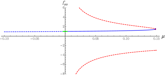
Figure 1: Real roots of (4) for different values of $\mu$. The lower red dashed line corresponds to $f_{\infty}<0$, whereas the upper one corresponds to unstable vacua; the blue dashed line ($\mu<0$) corresponds to stable vacua which do not allow for black hole solutions — see discussion under (16); the purple dot corresponds to the critical case, $\mu=4/27$; finally, the small green region corresponds to the set of parameters allowed by the positive-energy constraint $|t_{4}|\leq 4$ in (130).

We summarize these observations in Fig. 1, were we also include two additional constraints which we derive in sections 3 and 7.3, respectively. The first comes from imposing the existence of black holes solutions, which restricts the allowed values to $0\leq\mu\leq 4/27$. The second follows from the positivity of energy fluxes at null infinity which, as we can see from the figure, produces the very stringent constraint, $-0.00322\leq\mu\leq 0.00312$.

Throughout the paper, we will assume $\mu$ to lie in the range $0\leq\mu\leq 4/27$. From the two positive roots of (4) in that range, we will be implicitly choosing the one corresponding to a stable vacuum, which is also the one connecting to the Einstein gravity one for $\mu\rightarrow 0$. While the positive-energy condition further limits this range, we find it convenient to also consider values close to $\mu=4/27$, for which many exact results can be obtained. Let us finally point out that the solution of (4) corresponding to the relevant root (blue in Fig. 1) can be written explicitly as

$$f_{\infty}=\frac{2}{\sqrt{3\mu}}\sin\left[\frac{1}{3}\arcsin\left(\sqrt{\frac{27\mu}{4}}\right)\right]\,.$$ (8)

3 AdS₄ black holes

ECG admits static asymptotically AdS₄ black holes of the form

$$ds^{2}=-N^{2}V_{k}(r)dt^{2}+\frac{dr^{2}}{V_{k}(r)}+\frac{r^{2}}{L^{2}}d\Sigma_{k}^{2}\,,\quad\text{where}\quad d\Sigma_{k}^{2}=\begin{cases}L^{2}d\Omega^{2}_{2}\,,\quad&\text{for}\quad k=+1\,,\\ d\vec{x}_{2}^{2}\,,\quad&\text{for}\quad k=0\,,\\ L^{2}d\Xi^{2}\,,\quad&\text{for}\quad k=-1\,,\\ \end{cases}$$ (9)

corresponding to spherical, planar and hyperbolic horizons, respectively, and where $V_{k}(r)$ is determined from the second-order differential equation

$$1-\frac{L^{2}(V_{k}-k)}{r^{2}}-\frac{3L^{6}\mu}{4r^{3}}\left[\frac{V_{k}^{\prime 3}}{3}+\frac{kV_{k}^{\prime 2}}{r}-\frac{2V_{k}(V_{k}-k)V^{\prime}_{k}}{r^{2}}-\frac{V_{k}V_{k}^{\prime\prime}(rV^{\prime}_{k}-2(V_{k}-k))}{r}\right]=\frac{\omega^{3}}{r^{3}}\,,$$ (10)

where $\omega^{3}$ is an integration constant related to the ADM energy Abbott:1981ff ; Deser:2002jk of the solution — see (74). Also, $N^{2}$ is a constant that we fix in different ways depending on the horizon geometry, e.g., Quasi ; Myers:2010jv ; HoloRen . In particular, we will choose $N^{2}=1$ for spherical horizons, $N^{2}=1/f_{\infty}$ for planar horizons, which sets the speed of light in the dual theory to one, and $N^{2}=L^{2}/(f_{\infty}R^{2})$ for hyperbolic horizons, so that the boundary metric is conformally equivalent to that of $\mathbb{R}\times\mathbb{H}^{2}$, where $R$ is the curvature scale of the hyperbolic slices.

The fact that ECG admits static solutions of the form (9), characterized by a single function $V_{k}(r)$, such that the full nonlinear equations of the theory reduce to a single third-order differential equation, which can in turn be integrated once to yield (10), is a highly non-trivial property of ECG Hennigar:2016gkm ; PabloPablo2 . Such property is shared by the higher-dimensional Lovelock Wheeler:1985nh ; Wheeler:1985qd ; Boulware:1985wk ; Cai:2001dz ; Dehghani:2009zzb , QTG Quasi2 ; Quasi ; Dehghani:2011vu ; Cisterna:2017umf (for these, the equation for $V_{k}(r)$ is algebraic instead) and Generalized Quasi-topological Hennigar:2017ego gravities, as well as by other higher-curvature theories of the same class, recently discovered and characterized PabloPablo4 ; Ahmed:2017jod . As mentioned before, this property is related to the absence of extra modes in the linearized spectrum of the theory, and can be shown to lead to non-hairy black holes whose thermodynamic properties can be computed analytically on general grounds PabloPablo3 .

In (9), it is customary to make the redefinition

$$V_{k}(r)=k+\frac{r^{2}}{L^{2}}f(r)\,,$$ (11)

specially when dealing with the planar and hyperbolic cases. In terms of $f(r)$, (10) reads

$$1-f+\mu\left[f^{3}+\frac{3}{2}r^{2}ff^{\prime 2}-\frac{r^{3}}{4}f^{\prime}(f^{\prime 2}-3ff^{\prime\prime})+\frac{3}{4}kL^{2}f^{\prime}(rf^{\prime\prime}+3f^{\prime})\right]=\frac{\omega^{3}}{r^{3}}\,.$$ (12)

Observe that this reduces to (4) for constant $f(r)$ and $\omega^{3}=0$. In particular, asymptotically, we require $\lim_{r\rightarrow+\infty}f(r)=f_{\infty}$, which then makes (9) become the metric of pure AdS₄ with radius $\tilde{L}$ given by (3), and a different boundary geometry for each value of $k$ Emparan:1999pm .

3.1 Asymptotic expansion

For general values of $\mu$, finding analytic black hole solutions of (12) looks extremely challenging (if not impossible). Let us then start by exploring the asymptotic and near horizon expansions, from which we can gain a lot of relevant information (and, in fact, argue that non-hairy black hole solutions do really exist for general values of $\mu$).

The first terms in the asymptotic expansion of $f(r)$ read

$$f_{1/r}(r)=f_{\infty}-\frac{\omega^{3}}{(1-3\mu f_{\infty}^{2})r^{3}}-\frac{21\mu f_{\infty}\omega^{6}}{2(1-3\mu f_{\infty}^{2})^{3}r^{6}}+\mathcal{O}(r^{-8})\,.$$ (13)

Note that (12) is a second-order differential equation, which therefore possesses a two-parameter family of solutions. In order to capture the asymptotic behavior of the most general one, we write $f(r)=f_{1/r}(r)+h(r)$ and then expand (12) linearly in $h$. Keeping only leading terms in $1/r$, we get the following equation for $h$:

$$h^{\prime\prime}(r)-\frac{4(1-3\mu f_{\infty}^{2})^{2}}{9f_{\infty}\mu\omega^{3}}rh(r)=0\,.$$ (14)

Leaving aside the limiting cases, corresponding to $\mu=0$ and $\mu=4/27$, we see that there are two possibilities, depending on the sign of $\mu\cdot\omega^{3}$. If $\mu\cdot\omega^{3}>0$, (14) has the following approximate solutions as $r\rightarrow+\infty$:

$$h(r)\sim A\exp\left[\frac{4|1-3\mu f_{\infty}^{2}|}{9\sqrt{f_{\infty}\mu\cdot\omega^{3}}}r^{3/2}\right]+B\exp\left[-\frac{4|1-3\mu f_{\infty}^{2}|}{9\sqrt{f_{\infty}\mu\cdot\omega^{3}}}r^{3/2}\right]\,.$$ (15)

In order to obtain an asymptotically AdS₄ solution, we need to kill the growing mode, which forces us to set $A=0$. Therefore, this boundary condition fixes one of the integration constants required by (12). Now, even though the remaining exponentially decaying term is extremely subleading, in general we will have $B\neq 0$. In fact, this constant ends up being fixed by the horizon-regularity condition. In particular, this implies that the solutions show a strongly nonperturbative character, as $\sim e^{-1/\sqrt{\mu}}$ terms generically appear. Indeed, it is possible to show that a series expansion of the full solution in powers of $\mu$ is always divergent.

The second possibility corresponds to $\mu\cdot\omega^{3}<0$. An approximate solution of (14) for large $r$ is then given by

$$h(r)\sim\frac{A}{r}\cos\left[\frac{4|1-3\mu f_{\infty}^{2}|}{9\sqrt{f_{\infty}|\mu\cdot\omega^{3}|}}r^{3/2}\right]+\frac{B}{r}\sin\left[\frac{4|1-3\mu f_{\infty}^{2}|}{9\sqrt{f_{\infty}|\mu\cdot\omega^{3}|}}r^{3/2}\right]\,.$$ (16)

This solution is sick. Although $h(r)\rightarrow 0$ as $r\rightarrow+\infty$, the derivatives of $h$ diverge wildly in this limit, which would force us to set $A=B=0$ in order to get an asymptotically AdS₄ solution. However, this leaves us with no additional free parameters, and regularity at the (would-be) horizon cannot be imposed. Therefore, no regular black hole solution exists for $\mu\cdot\omega^{3}<0$: the solution is always sick, either at the horizon or at infinity.

As shown later in (74), $\omega^{3}$ is proportional to the total energy $E$ (or mass) of the black hole, which leads us to impose $\mu\geq 0$. Hence, interestingly, the range of values of $\mu$ which allows for positive-energy solutions, forbids the negative-energy ones, which simply do not exist for $\mu\geq 0$.

3.2 Near-horizon expansion

Let us now consider the near-horizon behavior. For that, we assume that there is a value ${r_{\rm\scriptscriptstyle H}}$ of the radial coordinate for which the function $V_{k}$ vanishes and is analytic. Analyticity ensures that the solution can be maximally extended beyond the horizon using Kruskal-Szekeres-like coordinates.

The derivative of $V_{k}$ at the horizon is related to the temperature through: $V_{k}^{\prime}({r_{\rm\scriptscriptstyle H}})=4\pi T/N$ so, in terms of $f$, the near-horizon expansion can be written as

$$k+\frac{r^{2}}{L^{2}}f(r)=\frac{4\pi T}{N}(r-{r_{\rm\scriptscriptstyle H}})+\sum_{n=2}^{\infty}a_{n}(r-{r_{\rm\scriptscriptstyle H}})^{n}\,,$$ (17)

where the relation between $f^{\prime}(r)$ and the temperature reads in turn

$$T=\frac{N}{4\pi}\left[\frac{{r_{\rm\scriptscriptstyle H}}^{2}}{L^{2}}f^{\prime}({r_{\rm\scriptscriptstyle H}})-\frac{2k}{{r_{\rm\scriptscriptstyle H}}}\right]\,.$$ (18)

Note also that $f({r_{\rm\scriptscriptstyle H}})=-kL^{2}/{r_{\rm\scriptscriptstyle H}}^{2}$. Now, if we plug (17) into (12) and we expand it in powers of $(r-{r_{\rm\scriptscriptstyle H}})$, we are led to the equation

$$0=1+\frac{kL^{2}}{{r_{\rm\scriptscriptstyle H}}^{2}}-\frac{\omega^{3}}{{r_{\rm\scriptscriptstyle H}}^{3}}-\frac{4L^{6}\pi^{2}T^{2}\mu}{N^{2}{r_{\rm\scriptscriptstyle H}}^{3}}\left(\frac{3k}{{r_{\rm\scriptscriptstyle H}}}+\frac{4\pi T}{N}\right)+\,$$ (19)

$$\left[-\frac{2kL^{2}}{{r_{\rm\scriptscriptstyle H}}^{2}}+\frac{3\omega^{3}}{{r_{\rm\scriptscriptstyle H}}^{3}}-\frac{4L^{2}\pi T}{N{r_{\rm\scriptscriptstyle H}}}+\frac{24L^{6}\pi^{2}T^{2}\mu}{N^{2}{r_{\rm\scriptscriptstyle H}}^{3}}\left(\frac{k}{{r_{\rm\scriptscriptstyle H}}}+\frac{2\pi T}{N}\right)\right](r-{r_{\rm\scriptscriptstyle H}})+\mathcal{O}\left((r-{r_{\rm\scriptscriptstyle H}})^{2}\right) \,.$$ (20)

Since every coefficient must vanish independently, we get an infinite number of equations relating the parameters in the near-horizon expansion (17). From the first two equations, we can obtain $T^{\rm ECG}$ and ${\omega}^{\rm ECG}$ as functions of ${r_{\rm\scriptscriptstyle H}}$, the result being (in order to minimize the clutter, we often omit the ‘ECG’ superscripts throughout the text)

$$T^{\rm ECG} =\frac{N}{2\pi{r_{\rm\scriptscriptstyle H}}}\left(k+\frac{3{r_{\rm\scriptscriptstyle H}}^{2}}{L^{2}}\right)\left[1+\sqrt{1+\frac{3kL^{4}\mu}{{r_{\rm\scriptscriptstyle H}}^{4}}\left(k+3\frac{{r_{\rm\scriptscriptstyle H}}^{2}}{L^{2}}\right)}\right]^{-1}\,,$$ (21)

$${(\omega^{\rm ECG})}^{3} =kL^{2}{r_{\rm\scriptscriptstyle H}}+{r_{\rm\scriptscriptstyle H}}^{3}-\frac{\mu L^{6}}{4}\left[\frac{3k}{{r_{\rm\scriptscriptstyle H}}}\left(\frac{4\pi T^{\rm ECG}}{N}\right)^{2}+\left(\frac{4\pi T^{\rm ECG}}{N}\right)^{3}\right]\,.$$ (22)

These reduce to the usual Einstein gravity results for $\mu=0$, namely

$$T^{\rm E}=\frac{N}{4\pi{r_{\rm\scriptscriptstyle H}}}\left(k+\frac{3{r_{\rm\scriptscriptstyle H}}^{2}}{L^{2}}\right)\,,\quad{(\omega^{\rm E})}^{3}={r_{\rm\scriptscriptstyle H}}^{3}+k{r_{\rm\scriptscriptstyle H}}L^{2}\,.$$ (23)

The rest of equations, which we do not show here, fix all coefficients $a_{n>2}$ in terms of $a_{2}$. Hence, for a fixed ${r_{\rm\scriptscriptstyle H}}$, the series (17) contains a single free parameter, which is nothing but the value of $f^{\prime\prime}$ at the horizon. This must be carefully chosen so that the solution has the appropriate asymptotic behavior, i.e., so that $A=0$ in (15).

3.3 Full solutions

Equation (12) can be solved analytically in two cases, namely: for Einstein gravity, $\mu=0$, and in the critical limit, $\mu=4/27$ Feng:2017tev . For those, one finds

$$f(r)=\begin{cases}1-\frac{{r_{\rm\scriptscriptstyle H}}^{3}+kL^{2}{r_{\rm\scriptscriptstyle H}}}{r^{3}}\quad{\rm\,\,if}\quad\mu=0\,,\\ \frac{3}{2}-\frac{3{r_{\rm\scriptscriptstyle H}}^{2}+2kL^{2}}{2r^{2}}\quad{\rm if}\quad\mu=4/27\,.\\ \end{cases}$$ (26)

For intermediate values of $\mu$, the solutions can be constructed numerically. In order to do so, we solve (12) setting the initial condition at the horizon, and then applying the shooting method to obtain the value of $a_{2}$ for which $f(r)\rightarrow f_{\infty}$. The differential equation (12) is very stiff when $r$ is large but, by choosing $a_{2}$ accurately, it is always possible to extend the numerical solution well into the region in which the asymptotic expression (13) applies. In all cases, there is a unique value of $a_{2}$ for which this happens. Hence, for each value of $\mu$ and each horizon geometry, there exists a unique regular black fully characterized by ${r_{\rm\scriptscriptstyle H}}$ (or, more physically, by $\omega^{\rm ECG}$).

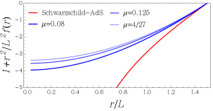
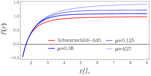
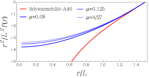
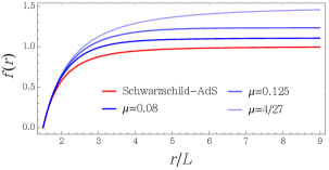
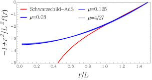
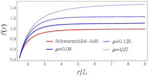
Figure 2: Black hole solutions for several values of $\mu$ (we take ${r_{\rm\scriptscriptstyle H}}=3L/2$), including the Einstein gravity ($\mu=0$) and critical ($\mu=4/27$) cases. From top to bottom $k=1,0,-1$. For the sake of clarity, we have made separate plots for the interior and exterior solutions. In the left column, we plot $V_{k}(r)=k+r^{2}/L^{2}f(r)$ for the black-hole interior range. In the right column we plot $f(r)$ instead for the exterior solutions.

In Fig. 2 we show a couple of these numerical solutions for ${r_{\rm\scriptscriptstyle H}}=1.5L$. As we can see, the corresponding curves lie between the analytic limiting solutions in (26). Far from the horizon, the functions $f(r)$ tend to the constant values $f_{\infty}$ which, as explained above, are different for each value of $\mu$ — see Fig. 1. Besides the exterior solutions, we also show plots of the black hole interior profiles, which present the curious feature of having regular metrics at $r=0$. However, as observed in PabloPablo2 for the asymptotically flat case, curvature invariants still diverge. For example, in the critical case, one finds

$$R_{abcd}R^{abcd}=\frac{4k^{2}L^{4}+54r^{4}-6{r_{\rm\scriptscriptstyle H}}^{2}r^{2}+{r_{\rm\scriptscriptstyle H}}^{4}-4kL^{2}(3r^{2}-{r_{\rm\scriptscriptstyle H}}^{2})}{L^{4}r^{4}}\sim\mathcal{O}\left(r^{-4}\right)\,,$$ (27)

which is two powers of $r$ softer than in the usual Schwarzschild case. Such behavior is common to all solutions with $\mu\neq 0$. This singularity-softening phenomenon appears to be generic for higher-curvature generalizations of Einstein gravity black holes. For example, for the Gauss-Bonnet black hole Cai:2001dz , one finds Ohta:2010ae $R_{abcd}R^{abcd}\sim\mathcal{O}(r^{-{(D-1)}})$, which is in turn $(D-1)$ powers of $r$ softer than the Kretschmann invariant of the $D$-dimensional Schwarzschild black hole.

4 Generalized action for higher-order gravities

When performing holographic calculations with higher-curvature bulk duals, one is faced with the challenge of identifying appropriate boundary terms which render the action differentiable, as well as counterterms which, along with those, give rise to finite and well-defined on-shell actions, when evaluated on stationary points of the functional. In this section, we propose a novel prescription for computing the on-shell action of arbitrary asymptotically AdS solutions of any $D$-dimensional higher-order gravity whose linearized spectrum on a maximally symmetric background matches that of Einstein gravity. The procedure represents an important simplification with respect to previous methods, as it only makes use of the usual Gibbons-Hawking-York boundary term and the counterterms of Einstein gravity. As we argue here — and illustrate throughout the rest of the paper and in appendix B with various non-trivial checks of the proposal — such contributions can be also used to produce the correct on-shell actions for this class of higher-order theories. Interestingly, for those, the only modification with respect to the Einstein gravity case is that such contributions appear weighted by the Lagrangian of the corresponding theory evaluated on the AdS background, i.e., $\mathcal{L}|_{{\rm AdS}}$. This quantity has been argued to be proportional to the charge $a^{*}$ appearing in the universal contribution to the entanglement entropy of the dual theory across a $\mathbb{S}^{d-2}$, and our prescription can be used to actually prove such a connection explicitly for this class of theories, as we show below.

Let us start considering a general higher-curvature theory of the form

$$I=\int_{\mathcal{M}}d^{D}x\sqrt{|g|}\mathcal{L}(g^{ef},R_{abcd})\,,$$ (28)

where the Lagrangian density $\mathcal{L}(g^{ef},R_{abcd})$ is assumed to be constructed from arbitrary contractions of the Riemann and metric tensors. The variation of the action with respect to the metric yields

$$\delta I=\int_{\mathcal{M}}d^{D}x\sqrt{|g|}\mathcal{E}_{ab}\delta g^{ab}+\epsilon\int_{\partial\mathcal{M}}d^{D-1}x\sqrt{|h|}n_{a}\delta v^{a}\,.$$ (29)

In this expression we defined

$$\mathcal{E}_{ab}\equiv P_{a}\,^{cde}R_{bcde}-\frac{1}{2}g_{ab}\mathcal{L}-2\nabla^{c}\nabla^{d}P_{acdb}\,,$$ (30)

the equations of motion reading $\mathcal{E}_{ab}=0$, and

$$\delta v^{a}=2g^{dc}P_{ed}^{\ \ ab}\nabla^{e}\delta g_{bc}\,,\quad\text{where}\quad P^{abcd}\equiv\left[\frac{\partial\mathcal{L}}{\partial R_{abcd}}\right]_{g^{ef}}\,.$$ (31)

In addition, $n^{a}$ is the unit normal to $\partial\mathcal{M}$, normalized as $n^{a}n_{a}\equiv\epsilon=\pm 1$, and $h_{ab}=g_{ab}-\epsilon n_{a}n_{b}$ is the induced metric. In order to have a well-posed variational problem, the action must be differentiable, in the sense that $\delta I\propto\delta g^{ab}$, so that $\delta I=0$ whenever the field equations — and the boundary conditions — are satisfied. This is not the case of (29), due to the presence of the boundary contribution. In the case of Einstein gravity, $\mathcal{L}^{\rm E}=\left[R+(D-1)(D-2)/L^{2}\right]/(16\pi G)$, this problem is solved by the addition of the Gibbons-Hawking-York term York:1972sj ; Gibbons:1976ue ,

$$I_{\rm GHY}=\frac{\epsilon}{8\pi G}\int_{\partial\mathcal{M}}d^{D-1}x\sqrt{|h|}K\,,$$ (32)

where $K=K_{ab}g^{ab}$ is the trace of the second fundamental form of the boundary, $K_{ab}=h_{a}^{\ c}\nabla_{c}n_{b}$. When this term is included, the variation of the action, when we keep $g_{ab}$ fixed at the boundary, reads

$$\delta(I^{\rm E}+I_{\rm GHY})\Big{|}_{\delta g_{ab}|_{\partial\mathcal{M}}=0}=\frac{1}{16\pi G}\int_{\mathcal{M}}d^{4}x\sqrt{|g|}\left[R_{ab}-\frac{1}{2}g_{ab}\mathcal{L}_{\rm EH}\right]\delta g^{ab}\,,$$ (33)

and so the action is stationary whenever the metric satisfies Einstein’s field equations.

For higher-order gravities, the situation is much more involved in general. One of the main issues arises from the fact that these theories generally posses fourth-order equations of motion. This implies that the boundary-value problem is not fully specified by the induced metric on $\partial\mathcal{M}$, and one needs to impose additional boundary conditions on derivatives of the metric. Furthermore, even if we know which components of the metric and its derivatives to fix, determining what boundary term needs to be added to yield a differentiable action for such variations is a far from trivial task. Some notable examples for which differentiable actions have been constructed are: quadratic gravities (perturbatively in the couplings) Smolic:2013gz , Lovelock gravities Teitelboim:1987zz ; Myers:1987yn , which are the most general theories with second-order covariantly-conserved field equations Lovelock1 ; Lovelock2 (and for which one only needs to fix $g_{ab}$ at the boundary), $f(R)$ Madsen:1989rz ; Dyer:2008hb ; Guarnizo:2010xr and, more generally, $f($Lovelock$)$ gravities Love . In these cases, it is also necessary to fix the value of some of the densities on the boundary — e.g., $\delta R\big{|}_{\partial\mathcal{M}}=0$ for $f(R)$ — which is related to the fact that these theories propagate additional scalar modes. With the goal of providing a canonical formulation for arbitrary $f$(Riemann$)$ gravities, an interesting proposal for constructing satisfactory boundary terms for such general class of theories was presented in Deruelle:2009zk — see also Teimouri:2016ulk . Unfortunately, the procedure involves the introduction of auxiliary fields and it is quite implicit in general, which seems to limit its practical applicability in the holographic framework.

The problem can be simplified if we specify the boundary structure in advance, e.g., by restricting the analysis to spacetimes which are maximally symmetric asymptotically. Let us, in particular, assume that the space is asymptotically AdS_D, so that the Riemann tensor behaves as $R_{abcd}\rightarrow-\tilde{L}^{-2}(g_{ac}g_{bd}-g_{ad}g_{bc})$ asymptotically. Then, on general grounds, the tensor $P_{cd}^{\ \ ab}$ appearing in the boundary term in (29) takes the simple form

$$P_{cd}^{\ \ ab}\rightarrow C(\tilde{L}^{2})\delta_{[c}^{\ a}\delta_{d]}^{\ b}+\text{subleading}\,,$$ (34)

where $C(\tilde{L}^{2})$ is a constant which depends on the background curvature, and is in general given by Aspects

$$C(\tilde{L}^{2})=-\frac{\tilde{L}^{2}}{2(D-1)}\mathcal{L}|_{{\rm AdS}}\,,$$ (36)

where $\mathcal{L}|_{{\rm AdS}}$ is the Lagrangian of the corresponding theory evaluated on the AdS_D background with curvature scale $\tilde{L}$.

For Einstein gravity, we simply have $C^{\rm E}=1/(16\pi G)$ and, in fact, there are no subleading terms in (34) for any spacetime — simply because $P_{cd}^{\ \ ab}$ only involves products of deltas in that case. Now, asymptotically AdS_D solutions of higher-order gravities will in general produce subleading contributions in (34) as we move away from the asymptotic region. However, the leading term can still be canceled out by adding a generalized GHY term of the form

$$I_{\rm GGHY}=2C(\tilde{L}^{2})\epsilon\int_{\partial\mathcal{M}}d^{D-1}x\sqrt{|h|}K\,.$$ (37)

The question is, of course, whether or not the subleading terms for a given theory will give additional non-vanishing contributions asymptotically, forcing us to add extra terms. We expect this to be the case in general. In addition, one generally needs to specify extra boundary conditions, which is related to the metric propagating additional degrees of freedom. However, as we have mentioned, some theories — see footnote 9 — do not propagate additional modes on general maximally symmetric backgrounds. For those, the asymptotic dynamics is the same as for Einstein gravity, so it is reasonable to expect the only data that we need to fix on $\partial\mathcal{M}$ to be $g_{ab}$, and also that (37) will be enough to make the action stationary for solutions of the field equations.

In order to obtain finite on-shell actions, one also needs to include counterterms, which only depend on the boundary induced metric. For asymptotically AdS_D spacetimes, there is a generic way of finding them Emparan:1999pm . Let us focus on Euclidean signature. In that case, we always have $\epsilon=+1$, and an additional global $(-)$ with respect to Lorentzian signature arises, e.g., Myers:2010tj , so we have

$$I_{E}=-\int_{\mathcal{M}}d^{D}x\sqrt{g}\mathcal{L}(g^{ef},R_{abcd})-2C(\tilde{L}^{2})\int_{\partial\mathcal{M}}d^{D-1}x\sqrt{|h|}K+I_{\rm GCT}\,,$$ (38)

where we seek to construct the generalized counterterms, $I_{\rm GCT}$. In order to identify all possible divergences, one possibility consists in evaluating the action on pure AdS_D spaces with different boundary geometries Yale:2011dq . Observe however that, whenever we evaluate the bulk term on pure AdS_D, this will produce an overall constant $\mathcal{L}|_{{\rm AdS}}$, which is precisely proportional to $C(\tilde{L}^{2})$. This already appears in front of the boundary term, and the result is that the combination of the bulk and boundary contributions reduce to those of Einstein gravity, up to a common overall $C(\tilde{L}^{2})$. Hence, the divergences are exactly the same as for Einstein gravity, and we can use the same counterterms. For example, up to $D=5$ we find Emparan:1999pm ; Yale:2011dq

$$I_{\rm GCT} =-2C(\tilde{L}^{2})\int_{\partial\mathcal{M}}d^{D-1}x\sqrt{h}\bigg{[}-\frac{D-2}{\tilde{L}}-\frac{\tilde{L}\Theta[D-4]}{2(D-3)}\mathcal{R}+\ldots\bigg{]}\,,$$ (39)

where $\Theta[x]=1$ if $x\geq 0$, and zero otherwise, and the dots refer to additional counterterms arising for $D\geq 6$. Combining (39) with (38), we obtain the final form of the action.

Below, we show that (38) successfully yields the right answers for ECG in various highly non-trivial situations in which the corresponding on-shell actions can be deduced from alternative considerations — e.g., it correctly computes the free energy of black holes, in agreement with the result obtained using Wald’s entropy, as well as the holographic stress tensor two-point charge, $C_{\scriptscriptstyle T}$, which can be alternatively deduced from the effective Newton constant. Besides, in appendix B we consider arbitrary radial perturbations of AdS₅ in Gauss-Bonnet gravity, and show that (38) produces exactly the same finite and divergent contributions as those obtained using the standard Gauss-Bonnet boundary term and counterterms, e.g., Teitelboim:1987zz ; Myers:1987yn ; Emparan:1999pm ; Mann:1999pc ; Balasubramanian:1999re ; Brihaye:2008xu ; Astefanesei:2008wz .

4.1 $a^{*}$ and generalized action

Let us momentarily switch to $d\equiv D-1$ notation. As we have seen, both the boundary term and the counterterms appearing in (38) have the property of being identical to those of Einstein gravity up to an overall constant $C(\tilde{L}^{2})$ proportional to the Lagrangian of the corresponding theory evaluated on the AdS background (36). Now, an interesting quantity that one would like to compute holographically is the charge $a^{*}$ appearing in the universal contribution to the entanglement entropy (EE) across a radius-$R$ spherical region $\mathbb{S}^{d-2}$ which, for a general CFT_d, is given by Myers:2010tj ; Myers:2010xs ; CHM

$$S_{\rm\scriptscriptstyle EE\,univ.}=\begin{cases}(-)^{\frac{d-2}{2}}4a^{*}\log(R/\delta)\quad&\text{for even }d\,,\\ (-)^{\frac{d-1}{2}}2\pi a^{*}\quad&\text{for odd }d\,.\end{cases}$$ (40)

$a^{*}$ coincides with the $a$-type trace-anomaly charge in even dimensional theories. In odd dimensions, $a^{*}$ is proportional to the free energy, $F=-\log Z$, of the corresponding theory evaluated on $\mathbb{S}^{d}$ CHM , namely

$$F_{\mathbb{S}^{d}}=(-)^{\frac{d+1}{2}}2\pi a^{*}\,,\quad\text{for odd }d\,.$$ (41)

For even-dimensional holographic theories dual to any higher-order gravity of the form (28) in the bulk, $a^{*}$ is given by Imbimbo:1999bj ; Schwimmer:2008yh

$$a^{*}=-\frac{\pi^{d/2}\tilde{L}^{d+1}}{d\Gamma(d/2)}\mathcal{L}|_{{\rm AdS}}\,,$$ (42)

i.e., it is precisely proportional to the charge $C(\tilde{L}^{2})$ defined in (36), namely

$$C(\tilde{L}^{2})=\frac{a^{*}}{\Omega_{(d-1)}\tilde{L}^{d-1}}\,,$$ (43)

where $\Omega_{(d-1)}\equiv 2\pi^{d/2}/\Gamma(d/2)$ is the area of the unit sphere $\mathbb{S}^{d-1}$. For odd-dimensional theories, it was argued in Myers:2010tj ; Myers:2010xs that (42) also yields the right $a^{*}$ for general cubic theories. We can readily extend this result to all theories for which (38) and (39) hold. From (41), it follows that $(-)^{\frac{d+1}{2}}2\pi a^{*}$ can be obtained from the on-shell action of pure Euclidean AdS_(d+1) with boundary geometry $\mathbb{S}^{d}$. Since $C(\tilde{L}^{2})$ appears as an overall factor in (38) when evaluated in pure AdS, it follows that $F_{\mathbb{S}^{d}}$ matches the Einstein gravity result up to an overall factor $16\pi G\cdot C(\tilde{L}^{2})$. Then, using the result for the free energy in Einstein gravity,

$$F^{\rm E}_{\mathbb{S}^{d}}=(-)^{\frac{d+1}{2}}\frac{\pi^{d/2}\tilde{L}^{d-1}}{4\Gamma(d/2)G}\,,$$ (44)

it follows immediately that for any theory of the form (28), for which our generalized on-shell action can be used,

$$F_{\mathbb{S}^{d}}=16\pi G\cdot C(\tilde{L}^{2})F^{\rm E}_{\mathbb{S}^{d}}=(-)^{\frac{d-1}{2}}\frac{2\pi^{d/2+1}\tilde{L}^{d+1}}{d\Gamma(d/2)}\mathcal{L}|_{{\rm AdS}}\,,$$ (45)

which takes the expected general form (41), with $a^{*}$ precisely given by (42). Hence, we have obtained the expected form of the charge $a^{*}$ from an explicit holographic calculation of the free energy on $\mathbb{S}^{d}$ using our generalized action. The consistency between (38) and (42) provides support for both expressions.

Reversing the logic, we can rewrite our generalized action in terms of $a^{*}$, which is way more charismatic than $C(\tilde{L}^{2})$. The result reads

$$I_{E}=-\int_{\mathcal{M}}d^{D}x\sqrt{g}\mathcal{L}(g^{ef},R_{abcd})-\frac{2a^{*}}{\Omega_{(d-1)}\tilde{L}^{d-1}}\int_{\partial\mathcal{M}}d^{D-1}x\sqrt{|h|}\left[K-\frac{d-1}{\tilde{L}}+\cdots\right]\,,$$ (46)

where we have omitted most of the counterterms in (39). The explicit appearance of $a^{*}$ in the boundary terms is rather suggestive, and somewhat striking. In section 9 we comment on the possible implications of (46) for holographic complexity.

4.2 Generalized action for Quasi-topological gravity

The QTG density in five bulk dimensions is given by Quasi2 ; Quasi

$$\mathcal{Z}_{5} =\tensor{R}{{}_{a}^{c}{}_{b}^{d}}\tensor{R}{{}_{c}^{e}{}_{d}^{f}}\tensor{R}{{}_{e}^{a}{}_{f}^{b}}+\frac{1}{56}\Big{(}-72\tensor{R}{{}_{abcd}}\tensor{R}{{}^{abc}_{e}}R^{de}+21\tensor{R}{{}_{abcd}}\tensor{R}{{}^{abcd}}R+120\tensor{R}{{}_{abcd}}\tensor{R}{{}^{ac}}\tensor{R}{{}^{bd}}$$ (47)

$$+144R^{b}_{a}R_{b}^{c}R_{c}^{a}-132R_{ab}R^{ab}R+15R^{3}\Big{)}\,.$$

Just like ECG in $D=4$, the linearized equations of this theory on constant-curvature backgrounds are Einstein-like Quasi . Hence, the method developed in the previous subsection should be valid for computing Euclidean on-shell actions of AdS₅ solutions of the theory. In this case, the full generalized action (46) is given by

$$I_{E}^{\rm QTG} =-\frac{1}{16\pi G}\int_{\mathcal{M}}d^{5}x\sqrt{g}\left[\frac{12}{L^{2}}+R+\frac{L^{2}\lambda}{2}\mathcal{X}_{4}+\frac{7\mu L^{4}}{4}\mathcal{Z}_{5}\right]$$ (48)

$$-\frac{1-6\lambda f_{\infty}+9\mu f_{\infty}^{2}}{8\pi G}\int_{\partial\mathcal{M}}d^{4}x\sqrt{h}\bigg{[}K-\frac{3\sqrt{f_{\infty}}}{L}-\frac{L}{4\sqrt{f_{\infty}}}\mathcal{R}\Bigg{]}\,,$$

where we also included the Gauss-Bonnet density $\mathcal{X}_{4}=R^{2}-4\tensor{R}{{}_{ab}}\tensor{R}{{}^{ab}}+\tensor{R}{{}_{abcd}}\tensor{R}{{}^{abcd}}$. In this case, the charge $a^{*}$ reads Myers:2010jv

$$a^{*{\rm QTG}}=\left(1-6\lambda f_{\infty}+9\mu f_{\infty}^{2}\right)\frac{\pi\tilde{L}^{3}}{8G}\,,$$ (49)

while $f_{\infty}$ is determined by the equation Quasi

$$1-f_{\infty}+\lambda f_{\infty}^{2}+\mu f_{\infty}^{3}=0\,.$$ (50)

A generalized boundary term for QTG was proposed in Dehghani:2011hm . It would be interesting to check whether (48) provides the same results as those obtained using such term. As we mentioned above, in appendix B we perform an explicit check of that kind for Gauss-Bonnet gravity.

4.3 Generalized action for Einsteinian cubic gravity

Let us now return to ECG. In that case, the full generalized Euclidean action (46) becomes

$$I_{E}^{\rm ECG}= -\frac{1}{16\pi G}\int d^{4}x\sqrt{|g|}\left[\frac{6}{L^{2}}+R-\frac{\mu L^{4}}{8}\mathcal{P}\right]$$ (51)

$$-\frac{1+3\mu f_{\infty}^{2}}{8\pi G}\int_{\partial\mathcal{M}}d^{3}x\sqrt{h}\left[K-\frac{2\sqrt{f_{\infty}}}{L}-\frac{L}{2\sqrt{f_{\infty}}}\mathcal{R}\right]\,,$$

where recall that $f_{\infty}$ can be obtained as a function of $\mu$ from (4). Observe also that the charge $a^{*}$ reads in this case

$$a^{*\rm ECG}=(1+3\mu f_{\infty}^{2})\frac{\tilde{L}^{2}}{4G}\,.$$ (52)

We use (51) in several occasions in the remainder of the paper, finding exact agreement with the expected results in all cases for which alternative methods can be used.

5 Stress tensor two-point function charge $C_{\scriptscriptstyle T}$

In order to characterize the holographic dual of ECG, we must translate the two available dimensionless parameters in (2), namely: $L^{2}/G$ and $\mu$, into universal defining quantities of the boundary theory. Since we are only considering the gravitational sector of the bulk theory, the most relevant ‘charges’ to be identified in the CFT are those characterizing the boundary stress tensor. Conformal symmetry highly constrains the structure of stress-tensor two- and three-point functions Osborn:1993cr . We will deal with the three-point function charges in section 7.3. Let us start here with the stress-tensor correlator which, for an arbitrary CFT₃, is given by Osborn:1993cr

$$\braket{T_{\mu\nu}(x)T_{\rho\sigma}(x^{\prime})}=\frac{C_{\scriptscriptstyle T}}{|x-x^{\prime}|^{6}}\mathcal{I}_{\mu\nu,\rho\sigma}(x-x^{\prime})\,,$$ (53)

where

$$\mathcal{I}_{\mu\nu,\rho\sigma}(x)\equiv\frac{1}{2}\left(I_{\mu\rho}(x)I_{\nu\sigma}(x)+I_{\mu\sigma}(x)I_{\nu\rho}(x)\right)-\frac{1}{4}\delta_{\mu\nu}\delta_{\rho\sigma}\,,\quad\text{and}\quad I_{\mu\nu}(x)\equiv\delta_{\mu\nu}-2\frac{x_{\mu}x_{\nu}}{x^{2}}\ ,$$ (54)

are fixed tensorial structures. This correlator is then fully characterized by a single theory-dependent parameter, customarily denoted $C_{\scriptscriptstyle T}$. This quantity, which in even dimensions is proportional to the trace anomaly charge $c$, also plays a relevant role in three-dimensional CFTs — see e.g., Huh:2014eea ; Diab:2016spb ; Giombi:2016fct for recent studies. As opposed to the $d=2$ case Zamolodchikov:1986gt , $C_{\scriptscriptstyle T}$ is not monotonous under general RG flows in three dimensional CFTs Nishioka:2013gza . However, it universally shows up in various contexts, including relevant quantities in entanglement and Rényi entropies HoloRen ; Hung:2014npa ; Perlmutter:2013gua ; Mezei:2014zla ; Bueno1 ; quantum critical transport — see e.g., Witczak-Krempa:2015pia ; Lucas:2017dqa and references therein; or partition functions on deformed curved manifolds Closset:2012ru ; Bobev:2017asb ; Fischetti:2017sut .

In AdS/CFT, the dual of $T_{\mu\nu}(x)$ is the normalizable mode of the metric Witten ; Gubser . Hence, evaluating (53) entails determining the two-point boundary correlator of gravitons in the corresponding AdS vacuum. For Einstein gravity in $d=3$, the result Buchel:2009sk ; Liu:1998bu reads

$$C_{\scriptscriptstyle T}^{{\rm E}}=\frac{3}{\pi^{3}}\frac{\tilde{L}^{2}}{G}\,.$$ (55)

Naturally, the introduction of higher curvature terms in the bulk modifies this result, e.g., Buchel:2009sk ; Myers:2010jv ; Bueno2 . In general, higher order gravities give rise to equations of motion involving more than two derivatives of the metric. In those cases, the metric generically contains additional degrees of freedom besides the usual massless graviton. From the holographic perspective, this means that the metric couples to additional operators which are typically nonunitary. This is not always the case, however. In fact, there exist families of higher order gravities whose linearized equations around maximally symmetric backgrounds are identical to those of Einstein gravity, up to a normalization of the Newton constant — see footnote 9 and e.g., Aspects for details. For those, the only mode is the usual spin-2 graviton, the metric only couples to the stress tensor, and $C_{\scriptscriptstyle T}$ can be straightforwardly extracted from the effective Newton constant. This generically reads $G_{\rm eff}=G/\alpha$, where $\alpha$ is a constant which depends on the new couplings. The appearance of $\alpha$ can be alternatively understood as changing the normalization of the graviton kinetic term which, holographically, gets translated into a modification of the stress-tensor correlator charge, which then becomes $\alpha\cdot C_{\scriptscriptstyle T}^{{\rm E}}$.

For ECG, using (7), we find then

$$C_{\scriptscriptstyle T}^{\rm ECG}=(1-3\mu f_{\infty}^{2})\frac{3}{\pi^{3}}\frac{\tilde{L}^{2}}{G}\,.$$ (56)

Observe that unitarity imposes $C_{\scriptscriptstyle T}$ to be positive, which translates into $1-3\mu f_{\infty}^{2}>0$. This is of course equivalent to asking the effective bulk gravitational constant to be positive. It can be seen that this constraint is automatically satisfied whenever (5) holds.

While we have been able to compute $C_{\scriptscriptstyle T}$ for ECG using $G_{\rm eff}^{\rm ECG}$, it is instructive to obtain it from an explicit holographic calculation. This will also serve as a highly-nontrivial consistency check for the new on-shell action method introduced in the previous section.

Let us then consider a metric perturbation: $g_{ab}=\bar{g}_{ab}+h_{ab}$, on the Euclidean AdS₄ vacuum

$$ds^{2}=\frac{r^{2}}{L^{2}}\left[d\tau^{2}+dx^{2}+dy^{2}\right]+\frac{L^{2}}{r^{2}f_{\infty}}dr^{2}\,.$$ (57)

Since all components of the two-point function will be determined by $C_{\scriptscriptstyle T}$, computing one of them will be enough. It is then sufficient to consider a perturbation of the form $h_{xy}=\frac{r^{2}}{L^{2}}\phi(r,\tau)$. Plugging this into the Euclidean version of (2) and expanding up to quadratic order in $\phi$, we find

$$I^{\rm ECG}_{E\,\rm\small Bulk}=\frac{(1-3\mu f_{\infty}^{2})}{32\pi G}\int d^{3}xdr\left[\frac{1}{\sqrt{f_{\infty}}}(\partial_{\tau}\phi)^{2}+\sqrt{f_{\infty}}\frac{r^{4}}{L^{4}}(\partial_{r}\phi)^{2}\right]-\frac{1}{16\pi G}\int d^{3}x\,\Gamma_{r}\Big{|}_{r=r_{\infty}}\,,$$ (58)

where $\Gamma_{r}$ is a boundary term which appears after integration by parts — see (180). Recall also that, in this coordinates, the boundary corresponds to $\lim_{r\rightarrow\infty}r\equiv L^{2}/\delta$, where we introduce the UV cutoff $\delta\ll 1$. The equation of motion for $\phi$ follows from (58), and reads

$$\frac{\partial}{\partial r}\left(\frac{r^{4}}{L^{4}}\frac{\partial\phi}{\partial r}\right)+\frac{1}{f_{\infty}}\frac{\partial^{2}\phi}{\partial\tau^{2}}=0\,.$$ (59)

In order to solve it, we Fourier-transform the dependence on the coordinate $\tau$,

$$\phi(r,\tau)=\frac{1}{2\pi}\int dp\phi_{0}(p)e^{ip\tau}H_{p}(r)\,.$$ (60)

$H_{p}$ satisfies the equation

$$\frac{d}{dr}\left(\frac{r^{4}}{L^{4}}\frac{dH_{p}}{dr}\right)-\frac{p^{2}}{f_{\infty}}H_{p}=0\,,$$ (61)

whose general solution reads

$$H_{p}(r)=c_{1}e^{-\frac{L^{2}|p|}{\sqrt{f_{\infty}}r}}\left(1+\frac{L^{2}|p|}{\sqrt{f_{\infty}}r}\right)+c_{2}e^{\frac{L^{2}|p|}{\sqrt{f_{\infty}}r}}\left(1-\frac{L^{2}|p|}{\sqrt{f_{\infty}}r}\right)\,.$$ (62)

In order to get a regular solution, we set $c_{2}=0$, and we also fix $c_{1}=1$ so that $H_{p}(r\rightarrow L^{2}/\delta)=1$. With this solution, we evaluate the Lagrangian, which can be expressed as a total derivative. Further integrating over the $r$ coordinate and substituting the solution in Fourier space, we get

$$I^{\rm ECG}_{E\,\rm\small Bulk}=\frac{\sqrt{f_{\infty}}V_{\mathbb{R}^{2}}}{64\pi^{2}G_{\rm eff}^{\rm ECG}}\int dpdq\phi_{0}(p)\phi_{0}(q)\delta(p+q)\frac{L^{4}}{\delta^{4}}H_{p}\partial_{r}H_{p}\Big{|}_{r=L^{2}/\delta}-\frac{1}{16\pi G}\int d^{3}x\Gamma_{r}\Big{|}_{r=L^{2}/\delta}\,,$$ (63)

where $V_{\mathbb{R}^{2}}=\int dxdy$, and where we used $\int d\tau e^{i(p+\tau)}=2\pi\delta(p+q)$.

Let us now turn to the boundary contributions in the generalized action (51). As we explain in appendix C, when these terms are added to (63), most divergences in $\Gamma_{r}\Big{|}_{r=L^{2}/\delta}$ disappear, and we are left with the following result for the full action:

$$I^{\rm ECG}_{E} =I^{\rm ECG}_{E\,\rm\small Bulk}+I^{\rm ECG}_{E\,\rm\small GGHY+GCT}$$ (64)

$$=\frac{V_{\mathbb{R}^{2}}}{64\pi^{2}G_{\rm eff}^{\rm ECG}\sqrt{f_{\infty}}}\int dpdq\phi_{0}(p)\phi_{0}(q)\delta(p+q)\left[f_{\infty}\frac{L^{4}}{\delta^{4}}H_{p}\partial_{r}H_{p}\Big{|}_{r=L^{2}/\delta}-\frac{L^{2}p^{2}}{\delta}H_{p}^{2}\right]\,.$$

Observe that, even though $1/G_{\rm eff}^{\rm ECG}$ and $a^{*\rm ECG}$ have a different dependence on $\mu$ — see (7) and (52) respectively — and that it is $a^{*\rm ECG}$ the one appearing as an overall constant in the generalized GHY term and the counterterms (51), everything conspires to produce a single finite contribution which is instead proportional to $1/G_{\rm eff}^{\rm ECG}$, as it must.

If we take the limit $\delta\rightarrow 0$ explicitly in (64), we get the simple result

$$I^{\rm ECG}_{E}[\phi_{0}]=-\frac{V_{\mathbb{R}^{2}}\tilde{L}^{2}}{64\pi^{2}G_{\rm eff}}\int dpdq\phi_{0}(p)\phi_{0}(q)\delta(p+q)|p|^{3}\,.$$ (65)

Using the holographic dictionary Witten , we can compute one of the components of the boundary stress tensor two-point function in momentum space as

$$\langle T_{xy}(0,0,p)T_{xy}(0,0,q)\rangle=-(2\pi)^{2}\frac{\delta^{2}I^{\rm ECG}_{E}[\phi_{0}]}{\delta\phi_{0}(-p)\delta\phi_{0}(-q)}=\frac{\tilde{L}^{2}V_{\mathbb{R}^{2}}}{8G_{\rm eff}}\delta(p+q)|p|^{3}\,.$$ (66)

Now, from the CFT side, this is given by

$$\langle T_{xy}(0,0,p)T_{xy}(0,0,q)\rangle=\int d^{3}x\int d^{3}x^{\prime}e^{-ip\tau}e^{-iq\tau^{\prime}}\langle T_{xy}(x)T_{xy}(x^{\prime})\rangle\,,$$ (67)

where

$$\langle T_{xy}(x)T_{xy}(x^{\prime})\rangle=\frac{C_{\scriptscriptstyle T}}{2|x-x^{\prime}|^{6}}\left[-1+2\frac{(\tau-\tau^{\prime})^{2}}{|x-x^{\prime}|^{2}}+8\frac{(x-x^{\prime})^{2}(y-y^{\prime})^{2}}{|x-x^{\prime}|^{4}}\right]\,.$$ (68)

The integration in (67) can be performed without further complications and we obtain the result

$$\langle T_{xy}(0,0,p)T_{xy}(0,0,q)\rangle=\frac{\pi^{3}C_{\scriptscriptstyle T}V_{\mathbb{R}^{2}}}{24}\delta(p+q)|p|^{3}\,.$$ (69)

Comparing this expression with (66), we obtain the result for $C_{\scriptscriptstyle T}$, which agrees with the one in (56), as it should. The fact that our generalized action (51) succeeds in providing the right answer for this quantity, including various non-trivial cancellations between $I^{\rm ECG}_{E\,\rm\small Bulk}$ and $I^{\rm ECG}_{E\,\rm\small GGHY+GCT}$ — see appendix C — provides strong evidence for the validity of the method developed in section 4.

Note finally that, as explained at the beginning of this section, $C_{\scriptscriptstyle T}$ provides information about many different physical quantities appearing in numerous contexts. Hence, by the same price we computed (56), we gain access to all such quantities for the CFT₃ dual to ECG.

6 Thermodynamics

In this section we study the thermodynamic properties of the ECG black holes constructed in section 3. First, we compute the Wald entropy, ADM energy and free energy of the solutions, and compare the result with the one obtained from an explicit on-shell action calculation, which serves as a further check of the method proposed in section 4. Then, focusing on the flat boundary case, $k=0$, we identify the quantity $C_{\scriptscriptstyle S}$ which relates the thermal entropy density to the temperature, and show that, in contradistinction to Einstein gravity, it defines an independent charge with respect to $C_{T}$. In subsections 6.3 and 6.4, we study the phase space of holographic ECG on $\mathbb{S}^{1}_{\beta}\times\mathbb{T}^{2}$ and $\mathbb{S}^{1}_{\beta}\times\mathbb{S}^{2}$, respectively. In the first case, we show that the standard phase transition between the ECG AdS soliton and black brane keeps occurring at the same temperature as for Einstein gravity. In the second, we show that depending on the value of $\mu$, one, two or three black hole solutions can coexist at the same temperature. The dominating phases are still thermal AdS at small temperatures and large black holes at large temperatures, but the Hawking-Page-transition temperature becomes arbitrarily large as we approach the critical limit $\mu=4/27$. Besides, small black holes become thermodynamically stable for $\mu\neq 0$, although their contribution to the partition function is always subleading with respect to thermal AdS.

6.1 Entropy, energy and free energy

Let us start by computing the Wald entropy of the solutions which, for any covariant theory of gravity is given by Wald:1993nt ; Iyer:1994ys

$$S=-2\pi\int_{\rm\scriptscriptstyle H}d^{d-1}x\,\sqrt{h}\frac{\partial\mathcal{L}}{\partial R^{ab}\,_{cd}}\varepsilon^{ab}\varepsilon_{cd}\,,$$ (70)

where $\varepsilon_{ab}$ is the binormal to the horizon. Now, for metrics of the form (9), the integration can be performed straightforwardly, yielding

$$S=-\frac{2\pi{r_{\rm\scriptscriptstyle H}}^{2}}{L^{2}}V_{\Sigma}\left.\frac{\partial\mathcal{L}^{\rm ECG}}{\partial R^{ab}\,_{cd}}\varepsilon^{ab}\varepsilon_{cd}\right|_{r={r_{\rm\scriptscriptstyle H}}}\,,$$ (71)

where $V_{\Sigma}$ is the regularized volume of $\mathbb{S}^{2}$, $\mathbb{R}^{2}$ or $\mathbb{H}^{2}$ for $k=1,0,-1$ respectively. Explicitly, the final result for the ECG black holes reads

$$S^{\rm ECG}=\frac{{r_{\rm\scriptscriptstyle H}}^{2}V_{\Sigma}}{4GL^{2}}\left[1-\frac{3\mu L^{4}\left(k+\frac{3{r_{\rm\scriptscriptstyle H}}^{2}}{L^{2}}\right)\left[\left(k+\frac{3{r_{\rm\scriptscriptstyle H}}^{2}}{L^{2}}\right)+2k\left[1+\sqrt{1+\frac{3kL^{4}\mu}{{r_{\rm\scriptscriptstyle H}}^{4}}\left(k+3\frac{{r_{\rm\scriptscriptstyle H}}^{2}}{L^{2}}\right)}\right]\right]}{{r_{\rm\scriptscriptstyle H}}^{4}\left[1+\sqrt{1+\frac{3kL^{4}\mu}{{r_{\rm\scriptscriptstyle H}}^{4}}\left(k+3\frac{{r_{\rm\scriptscriptstyle H}}^{2}}{L^{2}}\right)}\right]^{2}}\right]\,.$$ (72)

Again, this reduces to the Einstein gravity result

$$S^{\rm E}=\frac{{r_{\rm\scriptscriptstyle H}}^{2}V_{\Sigma}}{4GL^{2}}\,,$$ (73)

when we set $\mu=0$. Once we have $S(T)$ (defined implicitly), we can use the first law, $dE=TdS$, to find the energy. The result is

$$E^{\rm ECG}=\frac{{(\omega^{\rm ECG})}^{3}V_{\Sigma}N}{8\pi GL^{4}}\,.$$ (74)

As expected, this coincides with the result one would obtain for the generalized ADM energy from the asymptotic expansion (13).

The entropy of the solutions can be alternatively computed from the free energy as $S=-\partial F/\partial T$. Hence, we can perform an additional check of our generalized action (51), which evaluated on the Euclidean version of the solutions — for which we identify $t_{E}\sim t_{E}+\beta$ — should yield the free energy as $F^{\rm ECG}=I^{\rm ECG}_{E}/\beta$. Plugging (9) in (51), we find that the bulk term is a total derivative that can be integrated straightforwardly, namely

$$I^{\rm ECG}_{E\,{\rm Bulk}}=\frac{\beta NV_{\Sigma}}{16\pi GL^{2}}\left[H({r_{\rm\scriptscriptstyle H}})-H(L^{2}/\delta)\right]\,,$$ (75)

where

$$H(r)\equiv\frac{r^{3}}{L^{2}}\left[(2-4f-rf^{\prime})-\frac{\mu}{4}\left(2f+rf^{\prime}\right)^{2}\left(4f-rf^{\prime}\right)\right]\,.$$ (76)

Using the asymptotic expansion (13), we get

$$H(L^{2}/\delta)=\frac{2L^{4}}{\delta^{3}}(1-2f_{\infty}-2\mu f_{\infty}^{3})+\frac{{(\omega^{\rm ECG})}^{3}}{L^{2}}\frac{(1+3\mu f_{\infty}^{2})}{(1-3\mu f_{\infty}^{2})}+\mathcal{O}(\delta)\,.$$ (77)

We can also evaluate the boundary contributions in (51). For these, we use

$$d^{3}x\sqrt{h} =Ndt\wedge d\Sigma_{k}\left(\frac{\sqrt{f_{\infty}}L^{3}}{\delta^{3}}+\frac{kL}{2\delta\sqrt{f_{\infty}}}-\frac{{(\omega^{\rm ECG})}^{3}}{2\sqrt{f_{\infty}}L^{3}(1-3\mu f_{\infty}^{2})}\right)+\mathcal{O}(\delta)\,,$$ (78)

$$K =\frac{3\sqrt{f_{\infty}}}{L}+\frac{k\delta^{2}}{2L^{3}\sqrt{f_{\infty}}}+\mathcal{O}(\delta^{4})\,,\quad\mathcal{R}=\frac{2k\delta^{2}}{L^{4}}\,.$$

Then, we find

$$I^{\rm ECG}_{E\,\rm\small GGHY+GCT}=-\frac{\beta NV_{\Sigma}(1+3\mu f_{\infty}^{2})}{8\pi GL^{4}}\left[\frac{L^{6}f_{\infty}}{\delta^{3}}-\frac{{(\omega^{\rm ECG})}^{3}}{2(1-3\mu f_{\infty}^{2})}\right]+\mathcal{O}(\delta)\,.$$ (79)

Now, if we add up both contributions we obtain the finite result

$$I^{\rm ECG}_{E}=\frac{\beta NV_{\Sigma}}{16\pi GL^{2}}H({r_{\rm\scriptscriptstyle H}})\,,$$ (80)

where we made use of the AdS₄ embedding equation (4). Hence, all boundary contributions cancel out and the on-shell action is reduced to the evaluation of the function $H(r)$ at the horizon. Using the near-horizon expansion (17), we can finally write the free energy as

$$F^{\rm ECG}=\frac{NV_{\Sigma}}{8\pi GL^{2}}\left[k{r_{\rm\scriptscriptstyle H}}+\frac{{r_{\rm\scriptscriptstyle H}}^{3}}{L^{2}}-\frac{2\pi T{r_{\rm\scriptscriptstyle H}}^{2}}{N}+\mu L^{4}\left(\frac{3k}{{r_{\rm\scriptscriptstyle H}}}\left(\frac{2\pi T}{N}\right)^{2}+\left(\frac{2\pi T}{N}\right)^{3}\right)\right]\,.$$ (81)

Note that this can be also written fully in terms of ${r_{\rm\scriptscriptstyle H}}$ using (21). When $\mu=0$, (81) reduces to the Einstein gravity result

$$F^{\rm E}=\frac{NV_{\Sigma}{r_{\rm\scriptscriptstyle H}}}{16\pi GL^{2}}\left(k-\frac{{r_{\rm\scriptscriptstyle H}}^{2}}{L^{2}}\right)\,.$$ (82)

Using (81) and the thermodynamic identity $S=-\partial F/\partial T$, we can recompute the entropy of the solutions. The result precisely matches (72), computed using Wald’s formula, which provides another check for our generalized action.

6.2 Thermal entropy charge $C_{\scriptscriptstyle S}$

When the boundary geometry is flat, $k=0$, it is convenient to set $N^{2}=1/f_{\infty}$, a choice which fixes the speed of light to one in the dual CFT Buchel:2009sk . In that case, the thermodynamic expressions simplify considerably. In particular, we find

$$T=\frac{3{r_{\rm\scriptscriptstyle H}}}{4\pi L^{2}\sqrt{f_{\infty}}}\,,\quad{\omega}^{3}={r_{\rm\scriptscriptstyle H}}^{3}\left(1-\frac{27}{4}\mu\right)\,,$$ (83)

$$s=\frac{{r_{\rm\scriptscriptstyle H}}^{2}}{4GL^{2}}\left(1-\frac{27}{4}\mu\right)\,,\quad\varepsilon=\frac{{r_{\rm\scriptscriptstyle H}}^{3}}{8\pi GL^{4}\sqrt{f_{\infty}}}\left(1-\frac{27}{4}\mu\right)\,,$$ (84)

where we defined the entropy and energy densities $s\equiv S/V_{\mathbb{R}^{2}}$, $\varepsilon\equiv E/V_{\mathbb{R}^{2}}$. We can explicitly write these quantities in terms of the temperature, the result being

$$s=\frac{4\pi^{2}\tilde{L}^{2}f_{\infty}^{2}}{9G}\left(1-\frac{27}{4}\mu\right)T^{2}\,,\quad\varepsilon=\frac{8\pi^{2}\tilde{L}^{2}f_{\infty}^{2}}{27G}\left(1-\frac{27}{4}\mu\right)T^{3}.$$ (85)

From (85), it immediately follows that ECG black branes satisfy

$$\varepsilon=\frac{2}{3}Ts\,,$$ (86)

as expected for a thermal plasma in a general three-dimensional CFT.

The dependence on the temperature of the thermal entropy density is also fixed for any CFT₃ to take the form

$$s=C_{\scriptscriptstyle S}T^{2}\,,$$ (87)

where $C_{\scriptscriptstyle S}$ is a theory-dependent quantity. From, (85), it follows that

$$C_{\scriptscriptstyle S}^{\rm ECG}=\left(1-\frac{27}{4}\mu\right)f_{\infty}^{2}\,C_{\scriptscriptstyle{S}}^{\rm E}\,,\quad\text{where}\quad C_{\scriptscriptstyle{S}}^{\rm E}=\frac{4\pi^{2}}{9}\frac{\tilde{L}^{2}}{G}\,,$$ (88)

is the Einstein gravity result — see e.g., Buchel:2009sk . As we can see, in the holographic model defined by ECG, $C_{\scriptscriptstyle S}$ is no longer proportional to $C_{\scriptscriptstyle T}$, and therefore defines an additional well-defined independent ‘charge’ which characterizes the theory. For growing values of $\mu$, $C_{\scriptscriptstyle S}$ monotonously decreases with respect to the Einstein gravity value and, funnily, it vanishes for the critical case , $\mu=4/27$.

The fact that $C_{\scriptscriptstyle S}$ vanishes for certain value of the gravitational coupling is quite unusual, and does not occur for QTG or Lovelock black holes (in the Einstein gravity branch) in any number of dimensions — see e.g., Buchel:2009sk ; Quasi ; Myers:2010jv ; Dehghani:2009zzb ; Camanho:2011rj . In fact, in those cases, the only modification in $C_{\scriptscriptstyle S}$ with respect to Einstein gravity is an overall $f_{\infty}^{(d-1)}$ factor, i.e., the result reads $C_{\scriptscriptstyle S}^{\rm QTG/Lovelock}=f_{\infty}^{(d-1)}C_{\scriptscriptstyle{S}}^{\rm E}$, where $C_{\scriptscriptstyle{S}}^{\rm E}$ is the Einstein gravity result written in terms of $\tilde{L}$. In fact, in view of the results for those theories, one would have naively expected all ‘$(1-27/4\mu)$’ factors in (83)-(88) not to appear for ECG. This seems to be a simple manifestation of the fact that the theories belonging to the Generalized QTG class (including ECG) for which $f(r)$ is determined through a second-order differential equation possess rather different properties from those for which $f(r)$ is determined from an algebraic equation — see below and Hennigar:2017ego ; PabloPablo3 ; Ahmed:2017jod ; Hennigar:2017umz for more evidence in this direction.

6.3 Toroidal boundary: black brane vs AdS₄ soliton

In this subsection we study the phase space of thermal configurations when the spatial dimensions of the boundary CFT form a torus $\mathbb{T}^{2}$. The first obvious saddle corresponds to Euclidean AdS₄ with toroidal boundary conditions, given by

$$ds^{2}=\frac{r^{2}}{L^{2}}\left[d\tau^{2}+dx_{1}^{2}+dx_{2}^{2}\right]+\frac{L^{2}}{r^{2}f_{\infty}}dr^{2}\,,$$ (89)

where the coordinates $x_{1}$ and $x_{2}$ are assumed to be periodic, $x_{1,2}\sim x_{1,2}+l_{1,2}$, where $l_{1,2}$ is the period of each coordinate. Without loss of generality we assume $l_{1}\leq l_{2}$. As before, $\tau\sim\tau+\beta$. The next candidate is the Euclidean black brane

$$ds^{2}=\frac{r^{2}}{L^{2}}\left[\frac{f(r)}{f_{\infty}}d\tau^{2}+dx_{1}^{2}+dx_{2}^{2}\right]+\frac{L^{2}}{r^{2}f(r)}dr^{2}\,,$$ (90)

for which the temperature is fixed in terms of the horizon radius through (83). Finally, it should be evident that moving the $f(r)/f_{\infty}$ factor from $g_{\tau\tau}$ to $g_{11}$ or $g_{22}$ should also give rise to solutions of ECG, e.g.,

$$ds^{2}=\frac{r^{2}}{L^{2}}\left[d\tau^{2}+\frac{f(r)}{f_{\infty}}dx_{1}^{2}+dx_{2}^{2}\right]+\frac{L^{2}}{r^{2}f(r)}dr^{2}\,.$$ (91)

These are the so called AdS₄ ‘solitons’ Witten:1998zw ; Horowitz:1998ha . The crucial difference with respect to the black brane is that, for these, regularity no longer imposes a relation between the temperature and the horizon radius. Instead, it fixes the periodicity of $x_{1}$ (or $x_{2}$ if $f(r)/f_{\infty}$ appears in $g_{22}$ instead) in terms of ${r_{\rm\scriptscriptstyle H}}$ as

$$l_{1,2}=\frac{4\pi L^{2}\sqrt{f_{\infty}}}{3{r_{\rm\scriptscriptstyle H}}}\,.$$ (92)

Of course, $\tau$ is still periodic with period $\beta$, but, as opposed to the black-brane case, the temperature can be now arbitrary for a given value of ${r_{\rm\scriptscriptstyle H}}$.

Now, the Euclidean action vanishes for pure Euclidean AdS₄, whereas for the black brane and the solitons we find, respectively

$$I_{E}^{\rm bb}=-\frac{4\pi f_{\infty}L^{2}}{27G}\left(1-\frac{27}{4}\mu\right)T^{2}l_{1}l_{2}\,,\quad I_{E}^{\rm soliton\,1,2}=-\frac{4\pi f_{\infty}L^{2}}{27G}\left(1-\frac{27}{4}\mu\right)\frac{l_{1}l_{2}}{Tl_{1,2}^{3}}\,.$$ (93)

The solution which dominates the partition function is the one with the smaller on-shell action (or free energy, $\beta F\equiv I_{E}$). As we can see from (93), for the set of values of $\mu$ for which the ECG solutions exist, the free energies of the black brane and the AdS solitons are always negative, just like for Einstein gravity, which implies that pure AdS₄ never dominates. We observe that for (arbitrarily) small temperatures, the partition function is dominated by the soliton with the shortest periodicity, the other one being always subleading. For large temperatures, the black brane dominates instead. At $T=1/l_{1}$, (recall we are assuming $l_{1}<l_{2}$), there is a first-order phase transition which connects both phases. Hence, the phase-transition temperature is not modified with respect to Einstein gravity. The latent heat, computed as the difference between the energy densities of both configurations at $T=1/l_{1}$, does change and is given by

$$\delta Q=\frac{4\pi f_{\infty}L^{2}}{9G}\left(1-\frac{27}{4}\mu\right)\frac{l_{2}}{l_{1}^{2}}\,.$$ (94)

Again, something unusual happens in the critical limit. In that case, the free energy of both the black brane and the soliton — which have a simple metric function given by $f(r)=\frac{3}{2}(r^{2}-{r_{\rm\scriptscriptstyle H}}^{2})/L^{2}$ — vanishes. Then, for $\mu=4/27$, the black brane, the two solitons and pure AdS₄ are all equally probable configurations.

6.4 Spherical boundary: Hawking-Page transitions

Let us now consider the boundary theory on $\mathbb{S}^{1}_{\beta}\times\mathbb{S}^{2}$. In that case, apart from Euclidean AdS₄ foliated by spheres, the other candidate saddle of the semiclassical action corresponds to the Euclidean spherically symmetric black hole

$$ds^{2}=\left[1+\frac{r^{2}}{L^{2}}f(r)\right]d\tau^{2}+\frac{dr^{2}}{\left[1+\frac{r^{2}}{L^{2}}f(r)\right]}+r^{2}d\Omega^{2}_{(2)}\,,$$ (95)

where we have chosen $N^{2}=1$. Also, note that the ‘volume’ of the transverse space is, in this case, $V_{\mathbb{S}^{2}}=4\pi L^{2}$. As a function of the horizon radius, the temperature of these solutions is given by (21)

$$T({r_{\rm\scriptscriptstyle H}})=\frac{1}{2\pi{r_{\rm\scriptscriptstyle H}}}\left(1+3\frac{{r_{\rm\scriptscriptstyle H}}^{2}}{L^{2}}\right)\left[1+\sqrt{1+\frac{3\mu L^{4}}{{r_{\rm\scriptscriptstyle H}}^{4}}\left(1+3\frac{{r_{\rm\scriptscriptstyle H}}^{2}}{L^{2}}\right)}\right]^{-1}\ .$$ (96)

The contribution coming from the cubic term in the action becomes less and less relevant as we make ${r_{\rm\scriptscriptstyle H}}$ larger, but its effect is highly nonperturbative for small radius. For example, a non-vanishing value of $\mu$ makes the temperature vanish, instead of blowing up, as ${r_{\rm\scriptscriptstyle H}}\rightarrow 0$. More precisely, one finds $T\approx{r_{\rm\scriptscriptstyle H}}/(2\pi\sqrt{3\mu}L^{2})$ in that regime. This is no different from the behavior observed for the asymptotically flat ECG black holes Hennigar:2016gkm ; PabloPablo2 ; PabloPablo4 — small black holes do not care whether they are inside AdS₄ or flat space.

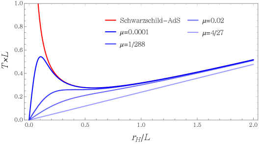
Figure 3: Temperature as a function of the horizon radius for various values of $\mu\in[0,4/27]$. Depending on $\mu$, there exist one, two, or three black holes with the same temperature.

Besides this, the introduction of the cubic term in the action leads to some additional differences with respect to Einstein gravity — see Fig. 3. For the usual Schwarzschild-AdS₄ Einstein gravity black hole, the temperature is always higher than a certain value, $T>T_{\rm min}\equiv\sqrt{3}/(2\pi L)$. In that case, for a given $T>T_{\rm min}$, there exist two black holes, one large, and one small. There are no solutions for which $T<T_{\rm min}$. For ECG the situation is quite different. On the one hand, one observes that there is no minimum temperature, this is, as long as $\mu\neq 0$, there always exists at least one black hole solution for a given $T$. We can distinguish two qualitatively different behaviors depending on $\mu$. For $0<\mu<\mu_{T}\equiv 1/288$, there is an interval of temperatures $\left(T_{\rm min},T_{\rm max}\right)$ for which three black hole solutions with the same temperature exist. However, if $T\geq T_{\rm max}$ or $T<T_{\rm min}$. we just have one. On the other hand, if $\mu>\mu_{T}$, there is always a single black hole solution for each temperature. In the critical limit, for which $f(r)=3(r^{2}-{r_{\rm\scriptscriptstyle H}}^{2})/(2L^{2})$, the relation (96) becomes linear Feng:2017tev , and reads $T=3{r_{\rm\scriptscriptstyle H}}/(4\pi L^{2})$.

In sum, at a fixed temperature $T$, we have several solutions with $\mathbb{S}^{1}_{\beta}\times\mathbb{S}^{2}$ boundary geometry: thermal AdS₄, and one or three black holes depending on the value of $\mu$. In order to identify which phase dominates the holographic partition function at each temperature, let us again compare the on-shell actions of the solutions. For thermal AdS₄, one finds a vanishing result, whereas for the black holes, the result can be obtained from (81), from which we can obtain $I_{E}(T)$ implicitly using (96).

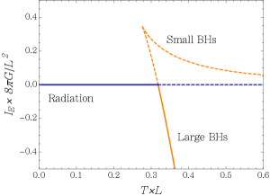
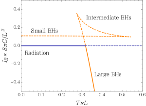
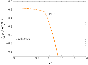
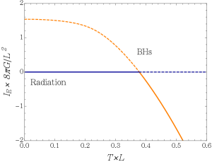
Figure 4: We plot $I_{E}$ as a function of the temperature for the different phases of holographic ECG in $\mathbb{S}^{1}_{\beta}\times\mathbb{S}^{2}$. Solid lines represent the dominant phase in each case. Blue lines correspond to thermal AdS₄, and orange lines to black holes. From left to right and top to bottom: $\mu=0,\,0.0001,\,1/288,\,0.02$. For $\mu=0$ we get the usual Einstein gravity result, with two orange branches corresponding to small and large black holes, and a Hawking-Page transition at $T_{\rm HP}=1/(\pi L)$. For $0<\mu<1/288$, there exist either one or three black-hole branches, depending on the temperature, while for $\mu>1/288$ there is a single black hole for every temperature. As $\mu$ approaches the critical value, the Hawking-Page transition temperature grows as $T_{\rm HP}\sim 3/(2\pi L\sqrt{1-27\mu/4})$. In the limit $\mu=4/27$, the on-shell action is constant (not shown in the figure), $I_{E}=4\pi L^{2}/(3G)$, so thermal AdS₄ always dominates, and there is no Hawking-Page transition.

In Fig. 4, we plot $I_{E}$ for various values of $\mu$. At a given temperature, we always have several possible phases: a pure thermal vacuum (radiation), and one or several black holes. The dominating phase (shown in solid line) is the one with smaller on-shell action. Regardless of the value of $\mu$, the qualitative behavior is always the same: for small temperatures, the partition function is dominated by radiation, while for large enough temperatures there is a Hawking-Page phase transition Hawking:1982dh ; Witten:1998zw to a large black hole. The temperature at which the transition occurs depends on $\mu$. For Einstein gravity, one finds $T_{\rm HP}=1/(\pi L)$, while for $\mu\ll 1$, this result gets corrected as

$$T_{\rm HP}=\frac{1+10\mu}{\pi L}+\mathcal{O}(\mu^{2})\,.$$ (97)

Hence, the introduction of the ECG density increases the temperature at which the transition occurs. The black-hole radius for which the phase transition takes place also grows if we turn on $\mu$, and is given by ${r_{\rm\scriptscriptstyle H}}=L(1+26\mu+\mathcal{O}(\mu^{2}))$, and the same happens with the latent heat, $\delta Q=L/G\cdot\left(1+38\mu+\mathcal{O}(\mu^{2})\right)$. As we increase $\mu$, the Hawking-Page transition temperature grows. In fact, it diverges in the critical limit $\mu=4/27$, which means that no transition at all occurs in that case. If we define $\epsilon\equiv 1-27/4\mu$, the transition temperature for $\epsilon\ll 1$ can be seen to be given by

$$T_{\rm HP}=\frac{3}{2\pi L\sqrt{\epsilon}}\left[1-\frac{\epsilon}{4}+\mathcal{O}(\epsilon^{2})\right]\,,\quad\text{which occurs for}\quad{r_{\rm\scriptscriptstyle H}}=\frac{2L}{\sqrt{\epsilon}}\left[1-\frac{1}{4}\epsilon+\mathcal{O}(\epsilon^{2})\right]\,.$$ (98)

The reason for the disappearance of the transition is that the critical black holes have a temperature-independent on-shell action, namely

$$I_{E}=\frac{4\pi L^{2}}{3G}\left[1-\frac{9+8\pi^{2}T^{2}L^{2}}{18}\epsilon+\mathcal{O}(\epsilon^{2})\right]\,,$$ (99)

which in the $\epsilon=0$ limit is a positive constant, therefore greater than the thermal AdS₄ value.

Although we have seen that only radiation and large black holes can dominate the partition function, it is worth stressing certain new features that appear in the thermal phase space of ECG. First, we observe that a low-temperature phase of small black holes becomes available as we turn on $\mu$. For small $T$, the corresponding on-shell action is given by

$$I_{E}^{\rm Small\,\,BHs}=\frac{2\pi L^{2}\sqrt{3\mu}}{G}\,.$$ (100)

Hence, if $\mu$ is small enough (but not zero!), a spontaneous transition from radiation to small black holes is likely to occur at low temperatures. However, a too small value of $\mu$ could be outside the limits of validity of this approach. Indeed, if the cubic corrections came from string theory, one would expect something like $\sqrt{\mu}L^{2}\sim\alpha^{\prime}$, which is assumed to be much larger than $G$ in the holographic setup. On the other hand, the phase space has a critical point (not to be confused with the critical limit of the theory) where the three black-hole phases in Fig. 4 (top right) stop existing separately. This occurs for $\mu=\mu_{T}$ which separates the cases for which there are three phases, from those for which there is only one. The phase transition is second-order, and takes place at a temperature $T_{\rm c}=\frac{\sqrt{2/3}}{\pi L}$, corresponding to the non-smooth point on the dashed orange curve in Fig. 4 bottom left. The critical exponent of the specific heat at the transition turns out to be $-2/3$. More precisely, we find

$$C\equiv-T\frac{\partial^{2}F}{\partial T^{2}}=\frac{\pi 5^{4/3}L^{2}}{9\cdot 2^{7/3}G}\left(\frac{T}{T_{\rm c}}-1\right)^{-2/3}\,\quad\text{as}\quad T\rightarrow T_{\rm c}\,.$$ (101)

Let us finally mention that the thermodynamic behavior of our black holes is qualitatively similar to the one observed for $D=5$ Gauss-Bonnet black holes Cai:2001dz . Just like for ECG, a new phase of small stable black holes appears also in that case, as a consequence of the Gauss-Bonnet term. Again, thermal AdS₅ is always globally preferred over such solutions. Observe also that the fact that there is no phase transition for critical ECG seems to be related to the fact that, in that case, the solutions become ‘very similar’ to three-dimensional BTZ black holes (see footnote 7), for which no Hawking-Page transition exists either Myung:2005ee . Finally, let us point out that more sophisticated phase transitions connecting different AdS vacua have been identified for Lovelock gravities in various dimensions Camanho:2013uda . It would be interesting to explore their possible existence in ECG or, more generally, for the class of theories introduced in Ahmed:2017jod ; PabloPablo4 ; Hennigar:2017ego .

7 Rényi entropy

Rényi entropies renyi1961 ; renyi1 are useful probes of the entanglement structure of quantum systems — see e.g., HoloRen ; Klebanov:2011uf ; Laflorencie:2015eck , and references therein. Roughly speaking, given a state $\rho$ and some spatial subregion $V$ in a QFT, Rényi entropies characterize ‘the degree of entanglement’ between the degrees of freedom in $V$ and those in its complement (when such a bi-partition of the Hilbert space is possible). More precisely, they are defined as

$$S_{q}(V)=\frac{1}{1-q}\log\operatorname{Tr}\rho_{V}^{q}\,,\quad q\geq 0\,,$$ (102)

where $\rho_{V}$ is the partial-trace density matrix obtained integrating over the degrees of freedom in the complement of the entangling region. Whenever (102) can be analytically continued to $q\in\mathbb{R}$, the corresponding EE can be recovered as the $q\rightarrow 1$ limit of $S_{q}$.

In this section we use the methods developed in CHM ; HoloRen to compute the Rényi entropy for disk regions in the ground state of holographic ECG. In subsection 7.1, we study the dependence of $S_{q}/S_{1}$ on $\mu$, as well as on some of the charges characterizing the CFT. In subsection 7.2, we compute the conformal scaling dimension of twist-operators $h_{q}$ for ECG — see below for definitions — as an intermediate step to obtain in subsection 7.3, using the results in Chu:2016tps , the charge $t_{4}$ characterizing the three-point function of the stress tensor.

7.1 Holographic Rényi entropy

In CHM , it was shown that the entanglement entropy across a radius-$R$ spherical region $\mathbb{S}^{d-2}$ for a generic $d$-dimensional CFT equals the thermal entropy of the theory at a temperature $T_{0}=1/(2\pi R)$ on the hyperbolic cylinder $\mathbb{R}\times\mathbb{H}^{d-1}$, where the curvature scale of the hyperbolic planes is given by $R$. The result is particularly useful in the holographic context, where the latter can be computed as the Wald entropy of pure AdS_(d+1) foliated by $\mathbb{R}\times\mathbb{H}^{d-1}$ slices. Later, in HoloRen , it was argued that this result could be in fact extended to general Rényi entropies, the result being

$$S_{q}=\frac{q}{(1-q)T_{0}}\int_{T_{0}/q}^{T_{0}}S_{\rm\scriptscriptstyle thermal}(T)dT\,,$$ (103)

where $S_{\rm\scriptscriptstyle thermal}(T)$ is the corresponding thermal entropy on $\mathbb{R}\times\mathbb{H}^{d-1}$ at temperature $T$. While for $T=T_{0}$, general results for the EE across a spherical region can be obtained for arbitrary holographic higher-derivative theories as long as AdS_(d+1) is a solution, the situation becomes more involved for general $q$. In that case, (103) requires that we know $S_{\rm\scriptscriptstyle thermal}(T)$ for arbitrary values of $T$. Holographically, the calculation can only be performed if the bulk theory admits hyperbolic black-hole solutions for which we are able to compute the corresponding thermal entropy. Examples of such theories for which Rényi entropies have been computed using this procedure include: Einstein gravity, Gauss-Bonnet, QTG HoloRen and cubic Lovelock Puletti:2017gym . Analogous studies for theories in which the corresponding black holes solutions were only accesible approximately — typically at leading order in the corresponding gravitational couplings — have also been performed, e.g., in Galante:2013wta ; Belin:2013dva ; Dey:2016pei . ECG allows us to perform the first exact calculation (fully nonperturbative in the gravitational couplings) of the holographic Rényi entropy of a disk region in $d=3$ for a bulk theory different from Einstein gravity.

Following HoloRen , let us start by rewriting (103) as

$$S_{q}=\frac{q}{(q-1)T_{0}}\left[\left.S(x)T(x)\right|^{1}_{x_{q}}-\int_{x_{q}}^{1}S^{\prime}(x)T(x)dx\right]\,,$$ (104)

where we defined the variable $x\equiv{r_{\rm\scriptscriptstyle H}}/\tilde{L}$, and where $S$ and $T$ stand for the thermal entropy and temperature of the hyperbolic AdS black hole of the corresponding theory. For $x=1$, one has, in general $T(1)=T_{0}$, whereas $x_{q}$ is defined as a solution to the equation $T(x_{q})=T_{0}/q$. For ECG cubic gravity, the expressions for $S(x)$ and $T(x)$ can be extracted from (72) and (21) respectively by setting $k=-1$,

$$S(x) =\frac{x^{2}\tilde{L}^{2}V_{\mathbb{H}^{2}}}{4G}\left[1-\frac{3\mu f_{\infty}^{2}\left(\frac{3x^{2}}{f_{\infty}}-1\right)\left[\left(\frac{3x^{2}}{f_{\infty}}-1\right)-2\left[1+\sqrt{1-\frac{3f_{\infty}^{2}\mu}{x^{4}}\left(\frac{3x^{2}}{f_{\infty}}-1\right)}\right]\right]}{x^{4}\left[1+\sqrt{1-\frac{3f_{\infty}^{2}\mu}{x^{4}}\left(\frac{3x^{2}}{f_{\infty}}-1\right)}\right]^{2}}\right]\,,$$

$$T(x) =\frac{1}{2\pi Rx}\left(\frac{3x^{2}}{f_{\infty}}-1\right)\left[1+\sqrt{1-\frac{3f_{\infty}^{2}\mu}{x^{4}}\left(\frac{3x^{2}}{f_{\infty}}-1\right)}\right]^{-1}\,,$$ (105)

where, in addition, we have set $N^{2}=L^{2}/(f_{\infty}R^{2})$. This makes the boundary metric conformally equivalent to

$$ds^{2}_{\rm bdy}=-dt^{2}+R^{2}d\Xi^{2}\,,$$ (106)

so that the boundary theory lives on $\mathbb{R}\times\mathbb{H}^{2}$, with the ‘radius’ of the hyperbolic plane given by $R$, as required HoloRen . From (105), it can be seen that $x_{q}$ corresponds to the real and positive solution of

$$x_{q}^{2}\left(3q^{2}x_{q}^{2}-q^{2}-2qx_{q}\right)=3\mu f^{2}_{\infty}\left(q^{2}x_{q}^{4}-1\right)\ ,$$ (107)

which for Einstein gravity reduces to

$$x^{\rm E}_{q}=\frac{1}{3q}\left(1+\sqrt{1+3q^{2}}\right)\ .$$ (108)

Observe that we have not said anything yet about the divergent nature of $V_{\mathbb{H}^{2}}$. Of course, one expects the entanglement and Rényi entropies to contain (a particular set of) divergent terms, so one could have only expected some source of divergences to appear in the calculation. It is a remarkably feature of the procedure outlined above that all necessary divergent terms in the Rényi entropy (and no others) are produced by the volume of the hyperbolic plane. In the case of interest for us, corresponding to $d=3$, the regularized volume reads CHM

$$V_{\mathbb{H}^{2}}=2\pi\left[\frac{R}{\delta}-1\right]\,,$$ (109)

where we introduced a short-distance cut-off $\delta$. From this expression, we shall only retain the universal piece, and hence we will replace $V_{\mathbb{H}^{2}}\rightarrow-2\pi$ from now on, keeping in mind that $S_{q}$ also contains a cut-off dependent ‘area’ law piece. Taking this into account, after some massaging, which includes using (4), we can check that

$$T(1)=T_{0}\,\quad\text{and}\quad S(1)=-2\pi a^{*\rm ECG}\,,$$ (110)

where $a^{*\rm ECG}$ was defined in (52). Hence, we obtain the same result for the EE of a disk as the one found in section 4 from the free energy of holographic ECG on $\mathbb{S}^{3}$. This is another check of our proposed generalized action (51).

With all the above information together, we are ready to evaluate the Rényi entropy from (104). The result reads

$$S^{\rm ECG}_{q}=\frac{q}{(1-q)}\frac{\pi\tilde{L}^{2}}{2G}\left[1-x_{q}-\frac{x^{2}_{q}}{q}+x_{q}^{3}-\mu f_{\infty}^{2}\left(\frac{3}{q^{2}x_{q}}-3-\frac{1}{q^{3}}+x_{q}^{3}\right)\right]\,,$$ (111)

which reduces to the Einstein gravity one HoloRen for $\mu=0$. In Fig. 5, we plot $S_{q}/S_{1}$ as a function of the Rényi index for various values of $\mu$.

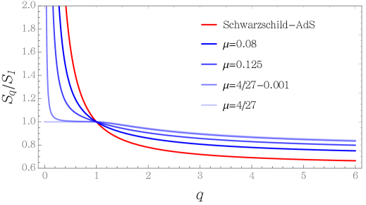
Figure 5: We plot the ratio of the Rényi entropy and the EE, $S_{q}/S_{1}$, as a function of the Rényi index $q$ for various values of the ECG coupling $\mu$.

As we increase $\mu$, $S_{q}/S_{1}$ becomes smaller in the $q<1$ region, but it remains larger than $1$ for all values of $\mu$. The opposite occurs for $q>1$, where $S_{q}/S_{1}$ tends to grow as we increase $\mu$, but $S_{q}/S_{1}<1$ for all $\mu$. In the critical limit, there is a jump, and $S_{q}/S_{1}$ no longer diverges near $q=0$. In fact, in that case, (111) reduces to a $q$-independent constant for $q<1$, $S^{\rm crit.\,ECG}_{q}=-\pi\tilde{L}^{2}/G$. As we approach $\mu\rightarrow 4/27$, $S_{\infty}$ tends to another constant, $S_{\infty}\rightarrow-\pi\tilde{L}^{2}/G\times(1-1/(3\sqrt{2}))$. Note also that the curve is no longer concave for $\mu\sim 0.135$ or larger.

Explicit Taylor expansions of $S^{\rm ECG}_{q}$ around $q=\{0,1,\infty\}$ can be easily obtained. A few terms suffice in such expansions to provide excellent approximations to the exact curve for most values of $\mu$. At leading order we find, respectively,

$$\lim_{q\rightarrow 1}S^{\rm ECG}_{q} = -2\pi a^{*\rm ECG}\ ,$$ (112)

$$\lim_{q\rightarrow 0}S^{\rm ECG}_{q} = -\frac{1}{6\pi q^{2}}C_{\scriptscriptstyle S}^{\rm ECG}\ ,$$ (113)

$$\lim_{q\rightarrow\infty}S^{\rm ECG}_{q} = -\frac{\pi\tilde{L}^{2}}{2G}\left[1+3\mu f^{2}_{\infty}-\frac{2}{3\sqrt{3(1-\mu f_{\infty}^{2})}}\right]\ .$$ (114)

The first result corresponds to the EE, and we have mentioned it already. As for the second, the appearance in the $q\rightarrow 0$ regime of the thermal entropy charge $C_{\scriptscriptstyle S}^{\rm ECG}$, identified in section 6.2, should not come as a surprise either. The reason is the following. As shown in HoloRen , the Rényi entropy $S_{q}$ across a $\mathbb{S}^{d-2}$ in a general CFT_d can be alternatively written as

$$S_{q}=\frac{q}{(1-q)}\frac{R^{d-1}V_{\mathbb{H}^{d-1}}}{T_{0}}\left[\mathcal{F}(T_{0})-\mathcal{F}(T_{0}/q)\right]\,,$$ (115)

where $\mathcal{F}(T)$ is the free energy density of the theory at temperature $T$ on $\mathbb{R}\times\mathbb{H}^{d-1}$. The point is that, as $q\rightarrow 0$, the second term in (115) dominates over the first. Then, one can use the fact that, at high temperatures, the free energy density on $\mathbb{R}\times\mathbb{H}^{d-1}$ tends to the free energy density on $\mathbb{R}^{d}$ Swingle:2013hga , $\mathcal{F}_{\mathbb{R}\times\mathbb{H}^{d-1}}(T)=\mathcal{F}_{\mathbb{R}^{d}}(T)\left[1+\mathcal{O}(1/(RT)^{2})\right]$, since $1/R$ becomes irrelevant compared to $T$ in that regime. Using the general relation $\mathcal{F}_{\mathbb{R}^{d}}(T)=-C_{\scriptscriptstyle S}T^{d}/d$, valid for any CFT in flat space, it follows then that

$$\lim_{q\rightarrow 0}S_{q}=\frac{V_{\mathbb{H}^{d-1}}C_{\scriptscriptstyle S}}{d}\left(\frac{1}{2\pi q}\right)^{d-1}\,,$$ (116)

which should hold for any CFT_d and, in particular, precisely agrees with (113) for ECG. Besides, we can readily check that

$$\left.\partial_{q}S^{\rm ECG}_{q}\right|_{q=1}=\frac{\pi^{4}}{12}C_{\scriptscriptstyle T}^{\rm ECG}\,,$$ (117)

as expected from the general relation found in Perlmutter:2013gua .

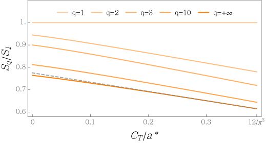
Figure 6: We plot the ratio of the Rényi entropy and the EE, $S_{q}/S_{1}$, as a function of the quotient $(C_{\scriptscriptstyle T}/a^{*})^{\rm ECG}$ for $q=\{1,2,3,10,\infty\}$. The limits of the range plotted correspond to the critical theory, $(C_{\scriptscriptstyle T}/a^{*})^{\rm ECG}=0$, and Einstein gravity $(C_{\scriptscriptstyle T}/a^{*})^{\rm ECG}=12/\pi^{3}$, respectively. The dashed line corresponds to the linear approximation to $S_{\infty}/S_{1}$ in (120).

Let us now gain some insight on the dependence of $S_{q}$ on quantities characterizing the CFT. In order to do that, we can use the relations

$$\frac{\tilde{L}^{2}}{G}=a^{*}\frac{\pi^{3}}{6}\left[(C_{\scriptscriptstyle T}/a^{*})+\frac{12}{\pi^{3}}\right]\,,\quad\mu f_{\infty}^{2}=-\frac{1}{3}\frac{\left[(C_{\scriptscriptstyle T}/a^{*})-\frac{12}{\pi^{3}}\right]}{\left[(C_{\scriptscriptstyle T}/a^{*})+\frac{12}{\pi^{3}}\right]}\,.$$ (118)

It is then straightforward to substitute these in (107) and (111) to obtain $S_{q}$ as a function of $a^{*\rm ECG}$ and $(C_{\scriptscriptstyle T}/a^{*})^{\rm ECG}$. Observe that $a^{*}$ appears as a global factor, so that $S_{q}/S_{1}$ is a function of $C_{\scriptscriptstyle T}/a^{*}$ alone. We plot this ratio for several values of $q$ in Fig. 6. Observe that $C_{\scriptscriptstyle T}/a^{*}$ takes values between $0$ and $12/\pi^{3}\simeq 0.3870$, corresponding to the critical value, $\mu=4/27$, and Einstein gravity respectively. Interestingly, even though the dependence of $S_{q}/S_{1}$ on $C_{\scriptscriptstyle T}/a^{*}$ is in principle highly non-linear, all curves seem to be approximately linear in the full range. In addition, we find that

$$\left.\frac{S_{q}}{S_{1}}\right|_{({C_{\scriptscriptstyle T}}_{1}/a_{1}^{*})}<\left.\frac{S_{q}}{S_{1}}\right|_{({C_{\scriptscriptstyle T}}_{2}/a_{2}^{*})}\,\quad\text{for}\quad({C_{\scriptscriptstyle T}}_{1}/a_{1}^{*})>({C_{\scriptscriptstyle T}}_{2}/a_{2}^{*})\,,$$ (119)

i.e., $S_{q}/S_{1}$ monotonously decreases as $C_{\scriptscriptstyle T}/a^{*}$ grows, for all values of $q$. These features are very similar to the ones observed in HoloRen for holographic Gauss-Bonnet in $d\geq 4$.

We can gain some understanding on the approximately linear behavior of $S_{q}/S_{1}$ by expanding $S_{\infty}/S_{1}$ around the Einstein gravity value, $(C_{\scriptscriptstyle T}/a^{*})^{\rm ECG}=12/\pi^{3}$. By doing so, we obtain

$$\frac{S_{\infty}}{S_{1}}=1-\frac{\pi^{3}\left[(C_{\scriptscriptstyle T}/a^{*})+\frac{12}{\pi^{3}}\right]^{3/2}}{72\left[(C_{\scriptscriptstyle T}/a^{*})+\frac{6}{\pi^{3}}\right]^{1/2}}\simeq\left[1-\frac{2}{3\sqrt{3}}\right]-\frac{5\pi^{3}}{216\sqrt{3}}\left[(C_{\scriptscriptstyle T}/a^{*})-\frac{12}{\pi^{3}}\right]+\dots\,,$$ (120)

where the first omitted correction is quadratic in the expansion parameter. As it turns out, the linear approximation in (120) fits the exact curve very well for most values of $C_{\scriptscriptstyle T}/a^{*}$ — see dashed line in Fig. 6. We suspect a similar phenomenon occurs for smaller values of $q$.

In spite of this ‘pseudo-linearity’, it seems clear that $S_{q}^{\rm ECG}$ does not have a simple dependence on universal CFT quantities. This fact, which agrees with the exact $d\geq 4$ results of HoloRen for Gauss-Bonnet and QTG, was actually anticipated in that paper also for $d=3$, where $S_{q}$ was computed at leading order in the gravitational coupling for a bulk model consisting of Einstein gravity plus a Weyl³ correction.

7.2 Scaling dimension of twist operators

Let us now turn to the scaling dimension of twist operators. In the context of computing Rényi entropies for some region $V$ using the replica trick, the boundary conditions which glue together the different copies of the replicated geometry at the entangling surface $\partial V$, can be alternatively implemented through the insertion of dimension-$(d-2)$ operators $\tau_{q}$ extending over $\partial V$ Calabrese:2004eu ; HoloRen ; Hung:2014npa ; Swingle:2010jz . The replicated-geometry construction is then replaced by a path integral over the symmetric product of $q$ copies of the theory on a single copy of the geometry, with the $\tau_{q}$ inserted. Given $V$, $\operatorname{Tr}\rho_{V}^{q}$ can be then obtained as the expectation value of these ‘twist operators’, $\operatorname{Tr}\rho_{V}^{q}=\braket{\tau_{q}}_{q}$, computed in the $q$-fold symmetric product CFT. A natural notion of scaling dimension, $h_{q}$, can be defined for $\tau_{q}$ from the leading singularity appearing in the correlator $\braket{T_{\mu\nu}\tau_{q}}$, as the stress tensor is inserted close to $\partial V$. In particular HoloRen ; Hung:2014npa ,

$$\braket{T_{\mu\nu}\tau_{q}}_{q}=-\frac{h_{q}}{2\pi}\frac{b_{\mu\nu}}{y^{d}}\,,$$ (121)

where $b_{\mu\nu}$ is a fixed tensorial structure and $y$ is the separation between the stress-tensor insertion and $\partial V$.

Our interest in the $h_{q}$ for ECG is mostly related to the use that we will make of them in the following subsection, so let us just reproduce the most relevant result needed to compute them for holographic CFTs HoloRen ; Hung:2014npa . This establishes that, given some higher-derivative bulk theory, $h_{q}$ can be obtained from the thermal entropy and temperature of the corresponding hyperbolic AdS black hole as

$$h_{q}=\frac{2\pi Rq}{(d-1)V_{\mathbb{H}^{d-1}}}\int_{x_{q}}^{1}T(x)S^{\prime}(x)dx\ .$$ (122)

Then, using (105), we find, for the universal piece,

$$h^{\rm ECG}_{q}=-\frac{q\tilde{L}^{2}}{8G}\left[x_{q}^{3}-x_{q}-\mu f^{2}_{\infty}\left(x_{q}^{3}+\frac{2}{q^{3}}-\frac{3}{q^{2}x_{q}}\right)\right]\ ,$$ (123)

which reduces to the Einstein gravity result HoloRen

$$h_{q}^{\rm E}=\frac{q\tilde{L}^{2}}{8G}x_{q}\left(1-x_{q}^{2}\right)\,,$$ (124)

when $\mu=0$. It is easy to perform some checks of this result. In particular, we find

$$\lim_{q\rightarrow 0}h^{\rm ECG}_{q}=-\frac{1}{12\pi^{2}q^{2}}C_{\scriptscriptstyle S}^{\rm ECG}\,,\quad\partial_{q}h^{\rm ECG}_{q}|_{q=1}=\frac{\pi^{3}}{24}C_{\scriptscriptstyle T}^{\rm ECG}\ ,$$ (125)

as expected from the general identities found in Bueno3 and Hung:2014npa , respectively. Similarly, using (111), it is possible to verify that the general relations Bueno3

$$\left.\partial^{j}_{q}h_{q}\right|_{q=1}=\frac{1}{4\pi}\left[(j+1)\left.\partial^{j}_{q}S_{q}\right|_{q=1}+j^{2}\left.\partial^{j-1}_{q}S_{q}\right|_{q=1}\right]\,,$$ (126)

hold for general $j$ and arbitrary values of $\mu$, as they should.

7.3 Stress tensor three-point function charge $t_{4}$

For general CFTs in $d=3$, the stress tensor three-point function is a combination of fixed tensorial structures controlled by two theory-dependent quantities Osborn:1993cr , which can be chosen to be $C_{\scriptscriptstyle T}$ plus an additional parameter, $t_{4}$. The latter was originally introduced in Hofman:2008ar , where it was shown to appear in the general formula for the energy flux reaching null infinity in a given direction after inserting an operator of the form $\epsilon_{ij}T^{ij}$, where $\vec{\epsilon}$ is some symmetric polarization vector. For any CFT₃, the result takes the general form

$$\braket{\mathcal{E}(\vec{n})}=\frac{E}{2\pi}\left[1+t_{4}\left(\frac{|\epsilon_{ij}n^{i}n^{j}|^{2}}{\epsilon_{ij}^{*}\epsilon_{ij}}-\frac{1}{8}\right)\right]\,,$$ (127)

where $E$ is the total energy, and $\vec{n}$ is the unit vector indicating the direction in which we are measuring the flux. Hence, the only theory-dependent quantity appearing in the above expression is $t_{4}$ which, along with $C_{\scriptscriptstyle T}$, fully characterize $\braket{TTT}$ — see e.g., Buchel:2009sk ; Bobev:2017asb for the explicit connection. For $d\geq 4$, there is an extra parity-preserving structure weighted by another theory-dependent constant, customarily denoted $t_{2}$.

Higher-dimensional versions of (127) have been used to identify $t_{4}$ and $t_{2}$ for holographic theories dual to certain higher-order gravities in $d\geq 4$, such as Lovelock Buchel:2009sk ; deBoer:2009gx or QTG Myers:2010jv . It is known that $t_{4}=0$ for general supersymmetric theories Hofman:2008ar ; Kulaxizi:2009pz , as well as for theories of the Lovelock class Buchel:2009sk ; deBoer:2009gx ; Camanho:2009hu ; Camanho:2013pda , including Einstein gravity in general dimensions. In fact, one of the original motivations for the construction of QTG in Quasi , was to provide a nonperturbative holographic model with a non-vanishing $t_{4}$ in $d=4$. Here, we show that ECG provides an analogous model in $d=3$.

In order to determine $t_{4}$ for ECG, we will use the results in Chu:2016tps , where it was shown that the scaling dimension of twist operators in holographic theories is related to the parameters controlling the stress-tensor three-point function. In particular, it was shown that the expression

$$\frac{h_{q}}{C_{\scriptscriptstyle T}}=\frac{\pi^{3}}{24}(q-1)-\frac{\pi^{3}}{11520}(420+t_{4})(q-1)^{2}+\mathcal{O}(q-1)^{3}\,,$$ (128)

holds for general holographic higher-order gravities in $d=3$, at least at leading order in the couplings. Performing the corresponding expansion in the twist-operator scaling dimension (123), we find

$$t^{\rm ECG}_{4}=\frac{-1260\mu f_{\infty}^{2}}{(1-3\mu f_{\infty}^{2})}\,,$$ (129)

which, as expected, vanishes for Einstein gravity. One may worry about the validity of (128) beyond leading order, for which $t_{4}^{\rm ECG}=-1260\mu+\mathcal{O}(\mu^{2})$. However, we have good reasons to believe that (129) is correct for general values of $\mu$. First of all, observe that (129) singles out $\mu=4/27$ as a special value of the coupling, since $t^{\rm ECG}_{4}$ diverges in that case. Of course, this is nothing but the critical limit of the theory, for which some sort of bizarre behavior was to be expected. Secondly, in appendix A, we use the results found in HoloRen for the twist-operator scaling dimensions in $d$-dimensional holographic Gauss-Bonnet and $d=4$ QTG, and show that the ($d$-dimensional versions of) (128) provide expressions for $t_{2}$ and $t_{4}$ which exactly agree with the fully nonperturbative ones found in Buchel:2009sk and Myers:2010jv . These observations strongly suggest that (129) is an exact expression.

Now, in $d=3$, imposing the positivity of energy fluxes in arbitrary directions gives rise to the constraint $-4\leq t_{4}\leq 4$, which is valid for general CFTs Buchel:2009sk , as long as the additional parity-odd structure is absent, as in the case of ECG. When written in terms of the gravitational coupling for ECG, this constraint translates into

$$\frac{312}{313}\leq f_{\infty}\leq\frac{318}{317}\,,$$ (130)

which, together with the previous constraint $1\leq f_{\infty}\leq 3/2$ becomes

$$1\leq f_{\infty}\leq\frac{318}{317}\simeq 1.00315\,.$$ (131)

This can in turn be explicitly written in terms of $\mu$ as

$$0\leq\mu\leq\frac{100489}{32157432}\simeq 0.00312491\,.$$ (132)

This reduces the range of allowed values of $\mu$ quite considerably. Observe that for $f_{\infty}=318/317$, $t_{4}=-4$, which is precisely the value corresponding to a free fermion. The other limiting value, $t_{4}=4$, corresponding to a free scalar, would imply a negative value of $\mu$, and is therefore excluded. Observe also that the bound is maximally violated at the critical value $\mu=4/27$.

8 Holographic hydrodynamics

One of the paradigmatic applications of higher-order gravities in the AdS/CFT context has been the construction of counterexamples to the famous Kovtun-Son-Starinets (KSS) bound for the shear viscosity over entropy density bound Kovtun:2004de . The latter was originally conjectured to satisfy $\eta/s\geq\frac{1}{4\pi}$ (in natural units) for any fluid in any number of dimensions, the saturation occurring for holographic plasmas dual to Einstein gravity AdS_(d+1) black branes. Violations of the bound — generically produced by finite-$N$ effects from the gauge-theory side — were argued to occur for holographic plasmas dual to black branes in several higher-order theories — see, e.g., Buchel:2004di ; Kats:2007mq ; Brigante:2007nu ; Myers:2008yi ; Cai:2008ph ; Ge:2008ni for some of the earliest works and Cremonini:2011iq for a review. A thorough study of various consistency conditions — such as subluminal propagation of excitations, energy positivity or unitarity — on some of the holographic theories for which the corresponding branes could be actually constructed — hence allowing for fully nonperturbative calculations in the higher-curvature couplings — suggested that the bound can be lowered down to $\eta/s\sim 0.4\cdot\frac{1}{4\pi}$ for $d=4$ Myers:2010jv , and arbitrarily close to zero for large enough $d$ Camanho:2010ru . These results give rise to three possibilities for finite-$d$: (i) the parameter space which would permit violations of the KSS bound is in fact not allowed by some other unidentified physical conditions — see below — and the KSS bound is true after all; (ii) there exists some lower bound, but it is lower than the KSS one; (iii) there is no bound at all. It was shown later Camanho:2014apa that higher-derivative theories with nonperturbative couplings are in fact generally acausal unless the spectrum is supplemented by higher-spin modes. While it is still unclear under what circumstances such additional degrees of freedom play a relevant role — specially given the success of holographic higher-curvature models in other holographic applications — the reliability of the aforementioned conclusions regarding the fate of the bound was put in suspense by this result. The current belief seems to be that some non-trivial bound, lower than the KSS one, does exist for general $d$ — see e.g., Fouxon:2008pz .

In this section we compute the shear viscosity to entropy density ratio for ECG, providing the first calculation of such a quantity for a holographic higher-curvature gravity in $d=3$ which is fully nonperturbative in the gravitational coupling. We will proceed along the lines of Myers:2010jv ; Paulos:2009yk . Let us start considering the ECG planar black hole in (9), i.e., we set $k=0$ and $N^{2}=1/f_{\infty}$,

$$ds^{2}=\frac{r^{2}}{L^{2}}\left[-\frac{f(r)}{f_{\infty}}dt^{2}+dx_{1}^{2}+dx_{2}^{2}\right]+\frac{L^{2}}{r^{2}f(r)}dr^{2}\,.$$ (133)

Now, it is convenient to perform the change of coordinates $z=1-{r_{\rm\scriptscriptstyle H}}^{2}/r^{2}$, so that the horizon corresponds to $z=0$, the asymptotic boundary being at $z=1$. The metric reads then

$$ds^{2}=\frac{{r_{\rm\scriptscriptstyle H}}^{2}}{L^{2}(1-z)}\left(-\frac{f(z)}{f_{\infty}}dt^{2}+dx_{1}^{2}+dx_{2}^{2}\right)+\frac{L^{2}}{4f(z)(1-z)^{2}}dz^{2}\,.$$ (134)

On the other hand, the cubic equation that determines $f(r)$, (12), reads, in terms of $z$

$$1-f(z)+\mu\left[f^{3}-3(1-z)^{2}ff^{\prime 2}-2(1-z)^{3}f^{\prime}(f^{\prime 2}-3ff^{\prime\prime})\right]=\left(1-\frac{27}{4}\mu\right)(1-z)^{3/2}\,,$$ (135)

where now $f^{\prime}\equiv df/dz$, and so on. In order to determine the shear viscosity, we will need the near-horizon behavior of $f$, so let us perform a Taylor expansion of the form

$$f(z)=f_{0}^{\prime}z+\frac{1}{2}f_{0}^{\prime\prime}z^{2}+\frac{1}{6}f_{0}^{\prime\prime\prime}(z)z^{3}+\dots,$$ (136)

The coefficients in this expansion can be of course written in terms of those in the $r$-expansion series (17), but it is easier to work directly with the variable $z$. Inserting (136) in (135) and imposing it to hold order by order in $z$, one finds

$$f_{0}^{\prime}=\frac{3}{2}\,,\quad f_{0}^{\prime\prime\prime}=\frac{-144\mu f_{0}^{\prime\prime 2}+4(135\mu+4)f_{0}^{\prime\prime}-81\mu+12}{216\mu}\,,\quad f_{0}^{(4)}=\ldots,$$ (137)

etc. All the coefficients are determined by $f_{0}^{\prime\prime}$, whose value is fixed by the asymptotic condition $\lim_{z\rightarrow 1}f(z)=f_{\infty}$. Analogously to the discussion in section 3.3, there is a unique value of this parameter for which the desired boundary condition is achieved. This defines $f_{0}^{\prime\prime}$ as a function of $\mu$, which we denote $f_{0}^{\prime\prime}(\mu)$. We can compute this numerically with arbitrary precision, but let us also try an analytic computation using the following logic. Observe that, for $\mu=0$, the solution is simply $f(z)=1-(1-z)^{3/2}$, from where we read all the derivatives

$$f_{0}^{(n)}(0)=(-1)^{n+1}\frac{\Gamma(5/2)}{\Gamma(5/2-n)}.$$ (138)

Now, since the solution for general $\mu$ should reduce to the Einstein gravity one when $\mu\rightarrow 0$, the derivatives (137) should coincide with the previous ones in that limit. It turns out that we can use this condition to determine the derivatives of $f_{0}^{\prime\prime}(\mu)$ with respect to $\mu$ at $\mu=0$. Let us see how this works. Obviously, we have $\lim_{\mu\rightarrow 0}f_{0}^{\prime\prime}(\mu)\equiv f_{0}^{\prime\prime}(0)=-3/4$. Then, we should also have $\lim_{\mu\rightarrow 0}f_{0}^{\prime\prime\prime}(\mu)\equiv f_{0}^{\prime\prime\prime}(0)=-3/8$. If we take this limit in the second equation of (137), we get the condition

$$\lim_{\mu\rightarrow 0}\left[\frac{-144f_{0}^{\prime\prime}(\mu)^{2}+540f_{0}^{\prime\prime}(\mu)-81}{216}+\frac{2}{27}\frac{f_{0}^{\prime\prime}(\mu)+3/4}{\mu}\right]=-\frac{3}{8}\,.$$ (139)

The limit of the first term is finite and we can simply substitute $f_{0}^{\prime\prime}(0)=-3/4$. However, in the second term we have

$$\lim_{\mu\rightarrow 0}\frac{f_{0}^{\prime\prime}(\mu)+3/4}{\mu}=\lim_{\mu\rightarrow 0}\frac{f_{0}^{\prime\prime}(\mu)-f_{0}^{\prime\prime}(0)}{\mu}\equiv\frac{df_{0}^{\prime\prime}(\mu)}{d\mu}\bigg{|}_{\mu=0}\,.$$ (140)

Therefore, this equation is actually giving us the value of the derivative of $f_{0}^{\prime\prime}(\mu)$ at $\mu=0$, the result being $243/8$. The same process can be repeated at every order and we can obtain all derivatives of this function at $\mu=0$. Up to second order, we have

$$f_{0}^{\prime\prime}(\mu=0)=-\frac{3}{4}\,,\quad\frac{df_{0}^{\prime\prime}(\mu)}{d\mu}\bigg{|}_{\mu=0}=\frac{243}{8}\,,\quad\frac{d^{2}f_{0}^{\prime\prime}(\mu)}{d\mu^{2}}\bigg{|}_{\mu=0}=-\frac{115911}{16}\,.$$ (141)

Now, if the function $f_{0}^{\prime\prime}(\mu)$ were analytic, we could in principle construct it as

$$f_{0}^{\prime\prime}(\mu)=\sum_{n=0}^{\infty}\frac{1}{n!}\frac{d^{n}f_{0}^{\prime\prime}(\mu)}{d\mu^{n}}\bigg{|}_{\mu=0}\mu^{n}\,.$$ (142)

However, a convergence analysis, including many terms in the expansion, reveals that this series is actually divergent for every $\mu\neq 0$ — in other words, the radius of convergence is 0. The fact that the series diverges is telling us that the function does not allow for a Taylor expansion around $\mu=0$. This is an example of a $\mathcal{C}^{\infty}$ function which is not analytic. Nevertheless, the series can be used to provide an approximate result for small enough $\mu$ if we truncate it at certain $n$. For example, to quadratic order we obtain

$$f_{0}^{\prime\prime}(\mu)\approx-\frac{3}{4}+\frac{243}{8}\mu-\frac{115911}{32}\mu^{2}\,,$$ (143)

but the approximation is only good for rather small values of the coupling, e.g., for $\mu=0.003$, the error is $\sim 3\%$ (with respect to the numerical value) and the precision is not increased by the addition of further terms. Observe also that in the critical limit, $\mu=4/27$, we have $f_{\rm cr}(z)=\frac{3}{2}z$, and hence $f_{0}^{\prime\prime}(4/27)=0$ in that case.

After this dissertation, which we will use to get a grasp on the small-$\mu$ behavior of $\eta$, let us now turn to the actual computation. In order to do so, we perturb the black hole metric (134) by shifting

$$dx_{1}\rightarrow dx_{1}+\varepsilon e^{-i\omega t}dx_{2}\,,$$ (144)

where $\varepsilon$ is a small parameter. Then, the shear viscosity can be obtained as Paulos:2009yk

$$\eta=-8\pi T\lim_{\omega,\epsilon\rightarrow 0}\frac{{\rm Res}_{z=0}\mathcal{L}}{\omega^{2}\epsilon^{2}}\,,$$ (145)

where $\mathcal{L}$ is the corresponding full gravitational Lagrangian (including the $\sqrt{|g|}$ term) in (2) evaluated on the perturbed metric. Using (136), we can evaluate this quantity, and the result reads

$$\eta^{\rm ECG}=\frac{3{r_{\rm\scriptscriptstyle H}}^{2}}{64\pi GL^{2}f_{0}^{\prime}}\left[2+(21f_{0}^{\prime 2}+36f_{0}^{\prime\prime 2}-114f_{0}^{\prime}f_{0}^{\prime\prime}+36f_{0}^{\prime}f_{0}^{\prime\prime\prime})\mu\right]\,.$$ (146)

Then, using the values of $f_{0}^{\prime}$ and $f_{0}^{\prime\prime\prime}$ in (137), we find

$$\eta^{\rm ECG}=\frac{{r_{\rm\scriptscriptstyle H}}^{2}}{32\pi GL^{2}}\left[5+27\mu+(4-36\mu)f_{0}^{\prime\prime}(\mu)\right]\,.$$ (147)

Finally, from (85) it follows that the shear viscosity over entropy density ratio reads

$$\left[\frac{\eta}{s}\right]^{\rm ECG}=\frac{5+27\mu+(4-36\mu)f_{0}^{\prime\prime}(\mu)}{8\pi\left(1-\frac{27}{4}\mu\right)}\,.$$ (148)

Some comments are in order. First, note that this expression is very different from the rest of nonperturbative results for $\eta/s$ available in the literature for $d\geq 4$ theories, corresponding to Lovelock Brigante:2007nu ; Ge:2009eh ; Brustein:2008cg ; Shu:2009ax and QTG Myers:2010jv . In those cases, it is found that $\eta/s$ depends on the gravitational couplings in a polynomial way — see also Parvizi:2017boc . On the contrary, the ECG result has a very nonpolynomial character, for two reasons. First, the presence of the function $f_{0}^{\prime\prime}(\mu)$, which is non-analytic, implies that $\eta/s$ cannot be Taylor-expanded around $\mu=0$. And second, the denominator ‘$(1-27/(4\mu))$’ in (148) is also a new feature, which gives rise to a divergence in the critical limit. The appearance of such contribution in the denominator is rooted in the different way in which ECG modifies the result for the thermal entropy charge $C_{\scriptscriptstyle S}$ with respect to the other theories mentioned above — see discussion in subsection 6.2.

Let us analyze the profile of $\eta/s$ as a function of $\mu$. When $\mu\ll 1$, we can use (143) to obtain

$$\left[\frac{\eta}{s}\right]^{\rm ECG}\approx\frac{1}{4\pi}\left(1+\frac{189\mu}{2}-\frac{114453\mu^{2}}{16}\right)\,.$$ (149)

Again, remember that, strictly speaking, this is not a Taylor expansion and it only provides a good approximation for very small $\mu$. In any case, note that the leading correction is positive, so $\eta/s$ is increasing with $\mu$. On the other hand, in the critical limit, we have $f_{0}^{\prime\prime}(\mu\rightarrow 4/27)\rightarrow 0$, so the leading behavior of $(\ref{eta/s})$ can be captured analytically,

$$\left[\frac{\eta}{s}\right]^{\rm ECG}=\frac{9}{8\pi\left(1-\frac{27}{4}\mu\right)}+\mathcal{O}(1)\,,\quad\text{for}\,\quad\mu\rightarrow\frac{4}{27}\,.$$ (150)

Hence, this ratio takes arbitrarily high values as we approach the critical limit. The full profile of $\eta/s$ can be obtained with arbitrary precision from a numerical computation of $f_{0}^{\prime\prime}(\mu)$. The result is shown in Fig. 7.

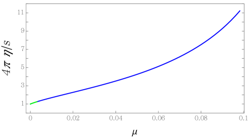
Figure 7: Shear viscosity to entropy density ratio as a function of $\mu$. The green line represents the region allowed by the constraint $t_{4}\geq-4$.

The curve is monotonically increasing, and blows up in the critical limit, $\mu=4/27$. Therefore, the KSS bound is not violated for any value of $\mu$ in the dynamically allowed region, $0\leq\mu\leq 4/27$, which is precisely a consequence of the nonexistence of $\mu<0$ solutions with positive energy. In that sense, as opposed to previously studied theories in higher dimensions, ECG simply does not allow for violations of the bound, not even in principle. It would be interesting to find out whether this phenomenon is common to the rest of $d=3$ theories constructed in PabloPablo4 and, more generally, to the new theories belonging to the Generalized QTG class Hennigar:2017ego ; PabloPablo3 ; Ahmed:2017jod in general dimensions.

As we explained in subsection 7.3, imposing the positivity of energy fluxes in the CFT, gives rise to the constraint $0\leq\mu\leq 0.00312$ — see green region in Fig. 7. This would imply a maximum possible value for $\eta/s$ in ECG, given by

$$\left[\frac{\eta}{s}\right]_{\rm max.}^{\rm ECG}\simeq 1.253\times\frac{1}{4\pi}\,.$$ (151)

From the results here, we can extract some general lessons regarding calculations of $\eta/s$ in higher-curvature holographic CFTs. First, we have seen that the ECG result is highly nonperturbative in the gravitational coupling. There is in principle no reason to expect this to be different for more general theories. The results found for Lovelock and QTG, polynomial in the gravitational couplings, are probably less generic — for those, the metric function $f(r)$ is determined by an algebraic equation, which is a highly exceptional property PabloPablo3 . Besides, as we have seen, there may be regions of the parameter space for which the corresponding black branes do not exist, even for arbitrarily small values of the couplings. None of this is seen when working perturbatively in the gravitational couplings, which means that the results obtained in that way must be taken carefully. This is a lesson which extends to most calculations in higher-curvature gravities.

9 Final comments

In this paper we have studied various aspects of $d=3$ holographic ECG, which, as we have argued, is a toy model of a nonsupersymmetric CFT ($t_{4}\neq 0$) analogous to QTG in $d=4$. A detailed summary of our findings can be found in subsection 1.1. We close the paper with a few additional comments.

Throughout the paper, we have computed several universal charges characterizing the dual CFT. In Table 1 we have collected some of them, as well as their $d=4$ QTG counterparts (with the Gauss-Bonnet coupling set to zero). For Einstein gravity, these are all proportional to the only dimensionless quantity present in the Lagrangian, namely, $\tilde{L}^{2}/G$. Just like for the higher-dimensional examples previously considered, including QTG, the introduction of the ECG coupling breaks this degeneracy, and all charges become independent from each other, in the sense that all possible ratios formed from them are $\mu$-dependent. As we can see, the stress-tensor parameters have remarkably similar numerical coefficients in both theories when expressed in terms of the Einstein-gravity charges. The expressions for $a^{*}$ are also similar, whereas the ones for $C_{\scriptscriptstyle S}$ are considerably different, due to the appearance of an extra factor which vanishes in the critical limit for ECG. The differences extend to many other quantities, as we have tried to illustrate throughout the text, which suggests that similar analyses for other members of the Generalized QTG family Hennigar:2017ego ; PabloPablo3 ; Ahmed:2017jod ; PabloPablo4 should be performed. In particular, it would be interesting to find out whether the highly-nonperturbative result for the shear viscosity over entropy density ratio extends to those theories, and whether violations of the KSS bound are also forbidden for them.

	$C_{\scriptscriptstyle T}$	$C_{\scriptscriptstyle T}\cdot t_{4}$	$C_{\scriptscriptstyle S}$	$a^{*}$
Einstein	$\frac{\Gamma(d+2)}{8(d-1)\Gamma(d/2)\pi^{(d+2)/2}}\frac{\tilde{L}^{d-1}}{G}$	$0$	$\frac{\Gamma(d+1)\pi^{(2d-1)/2}2^{d-3}}{\Gamma(\frac{d+1}{2})\Gamma(d/2)d^{d}}\frac{\tilde{L}^{d-1}}{G}$	$\frac{\pi^{(d-2)/2}}{8\Gamma(d/2)}\frac{\tilde{L}^{d-1}}{G}$
ECG $(d=3)$	$(1-3\mu f_{\infty}^{2})C_{\scriptscriptstyle T}^{{\rm E}}$	-$1260\mu f_{\infty}^{2}C_{\scriptscriptstyle T}^{{\rm E}}$	$\left(1-\frac{27}{4}\mu\right)f_{\infty}^{2}C_{\scriptscriptstyle{S}}^{\rm E}$	$\left(1+3\mu f_{\infty}^{2}\right)a^{*{\rm\scriptscriptstyle E}}$
QTG $(d=4)$	$(1-3\mu f_{\infty}^{2})C_{\scriptscriptstyle T}^{{\rm E}}$	$3780\mu f_{\infty}^{2}C_{\scriptscriptstyle T}^{{\rm E}}$	$f_{\infty}^{3}C_{\scriptscriptstyle{S}}^{\rm E}$	$\left(1+9\mu f_{\infty}^{2}\right)a^{*{\rm\scriptscriptstyle E}}$

Table 1: From left to right: stress-tensor two- and three-point function charges $C_{\scriptscriptstyle T}$ and $C_{\scriptscriptstyle T}\cdot t_{4}$, thermal entropy charge $C_{\scriptscriptstyle S}$, and universal contribution to the entanglement entropy across a spherical region, $a^{*}$, for holographic theories dual to Einstein gravity in $d$ dimensions, ECG ($d=3$) and Quasi-topological gravity (with vanishing Gauss-Bonnet coupling) in $d=4$ Myers:2010jv .

9.1 Generalized action, $a^{*}$ and holographic complexity?

In section 4, we proposed a new method for evaluating Euclidean on-shell actions for higher-order gravities whose linearized equations of motion on maximally symmetric backgrounds are second order. Throughout the paper, we have performed several successful and highly non-trivial checks of the proposal — see appendix B as well. It would be interesting to perform further studies of our generalized action (38) for other theories, such as higher-order Lovelock theories, QTG and its higher-order generalizations and, more generally, for theories of the Generalized QTG type. One of the most striking aspects of (38) is that it avoids the — usually very challenging — problem of determining the correct generalization of the Gibbons-Hawking-York boundary term. At the same time, and somewhat surprisingly, it involves the universal charge $a^{*}$ controlling the EE of spherical regions in the corresponding dual CFT. This acts as a weight that changes from one theory to another.

As pointed out in Carmi:2016wjl , one of the open questions in the context of holographic complexity, is to determine what kind of universal information (if any) is encoded in the results obtained using the ‘complexity$=$volume’ Susskind:2014rva ; Stanford:2014jda and ‘complexity$=$action’ Brown:2015bva ; Brown:2015lvg prescriptions. In order to do so, one possible venue would consist in studying the corresponding quantities for holographic higher-order gravities. For those, the charge-degeneracy inherent to Einstein gravity (where all charges are proportional to $\tilde{L}^{2}/G$) is broken, and one would hope to be able to identify the nature of possible universal quantities appearing in holographic complexity. Our generalized action (38) suggests that $a^{*}$ may appear universally in some of these terms. Observe that complexity$=$action calculations require the introduction of additional terms in the gravitational action when the boundary contains null pieces and joints — see Lehner:2016vdi and references therein. In that case one can only speculate on whether a similar mechanism could make $a^{*}$ — or some other characteristic charge — appear in the corresponding generalized terms for higher-order gravities.

Appendix A $\braket{TTT}$ parameters from $h_{q}$

In this appendix we show that the formulas in Chu:2016tps for the twist operator scaling dimensions $h_{q}$ around $q=1$ can be used to obtain the exact values of the parameters $t_{2}$ and $t_{4}$ for holographic Gauss-Bonnet in general dimensions, and for QTG in $d=4$. The general-$d$ version of (128) reads Chu:2016tps

$$\frac{h_{q}}{C_{\scriptscriptstyle T}}=2\pi^{\frac{d}{2}+1}\frac{\Gamma(d/2)}{\Gamma(d+2)}(q-1)+\frac{h^{\prime\prime}_{q}(1)}{2C_{\scriptscriptstyle T}}(q-1)^{2}+\mathcal{O}(q-1)^{3}\ ,$$ (152)

where

$$\frac{h^{\prime\prime}_{q}(1)}{C_{\scriptscriptstyle T}}= -\frac{2\pi^{1+d/2}\Gamma(d/2)}{(d-1)^{3}d(d+1)\Gamma(d+3)}\Bigg{[}d\left(2d^{5}-9d^{3}+2d^{2}+7d-2\right)$$ (153)

$$+(d-2)(d-3)(d+1)(d+2)(2d-1)t_{2}+(d-2)(7d^{3}-19d^{2}-8d+8)t_{4}\Bigg{]}\ .$$

This expression is valid for general holographic higher-order gravities, at least at leading order in the gravitational couplings.

A.1 Gauss-Bonnet in arbitrary dimensions

In this case, the expression for the scaling dimension of twist operators is given by HoloRen

$$\frac{h_{q}}{C_{\scriptscriptstyle T}}=\frac{\Gamma(d/2)}{4\Gamma(d+2)}\pi^{1+d/2}qx_{q}^{d-4}(x_{q}^{2}-1)\left[d-3-(d+1)x_{q}^{2}+(d-3)\frac{1-2\frac{d-1}{d-3}\lambda f_{\infty}}{1-2\lambda f_{\infty}}(x_{q}^{2}-1)\right]\,,$$ (154)

where $x_{q}$ satisfies the following quartic equation

$$x_{q}^{4}d-\frac{2}{q}x_{q}^{3}-(d-2)x_{q}^{2}+\lambda f_{\infty}\left[4\frac{x_{q}}{q}-x_{q}^{4}d+d-4\right]=0\,.$$ (155)

A Taylor expansion around $q=1$ gives

$$x_{q}=1+\frac{1}{1-d}(q-1)+\frac{d}{(d-1)^{3}}\frac{-2d+3+\lambda f_{\infty}(4d-10)}{-2+4\lambda f_{\infty}}(q-1)^{2}+\mathcal{O}(q-1)^{3}\,.$$ (156)

Plugging this expansion into (154), we find

$$\frac{h_{q}}{C_{\scriptscriptstyle T}}=\frac{2\Gamma(d/2)\pi^{1+d/2}}{\Gamma(d+2)}(q-1)$$ (157)

$$-\frac{(d-1)\Gamma(d/2)\pi^{1+d/2}}{\Gamma(d+2)}\left[-1+4d-2d^{2}+\lambda f_{\infty}(6-16d+4d^{2})\right](q-1)^{2}+\mathcal{O}(q-1)^{3}\,.$$

Comparing this with (152), we find that $t_{2}$ and $t_{4}$ should be given by

$$t_{2}=\frac{4d(d-1)\lambda f_{\infty}}{(d-2)(d-3)(1-2\lambda f_{\infty})}\,,\quad t_{4}=0\,,$$ (158)

which matches the exact nonperturbative result Buchel:2009sk .

A.2 Quasi-topological gravity

In this case, the scaling dimension $h_{q}$ was obtained in HoloRen in terms of the charges $a$, $c$ and $t_{4}$ of the theory as

$$h_{q}=\frac{aq}{4\pi x_{q}^{2}}(x_{q}^{2}-1)\left[x_{q}^{4}\left(1-5\frac{c}{a}-10\frac{c}{a}t_{4}\right)-x_{q}^{2}\left(1-\frac{c}{a}-8\frac{c}{a}t_{4}\right)+2\frac{c}{a}t_{4}\right]\ ,$$ (159)

where

$$c = \pi^{2}\frac{\tilde{L}^{3}}{8\pi G}\left(1-2\lambda f_{\infty}-3\mu f_{\infty}^{2}\right)\ ,$$ (160)

$$a = \pi^{2}\frac{\tilde{L}^{3}}{8\pi G}\left(1-6\lambda f_{\infty}+9\mu f_{\infty}^{2}\right)\ ,$$ (161)

$$t_{4} = \frac{3780\mu f_{\infty}^{2}}{1-2\lambda f_{\infty}-3\mu f_{\infty}^{2}}\ ,$$ (162)

and where $x_{q}$ satisfies the following quartic equation

$$2x_{q}^{6}-\frac{x_{q}^{5}}{q}-x_{q}^{4}+2\lambda f_{\infty}x_{q}^{3}\left(\frac{1}{q}-x_{q}^{3}\right)+\mu f_{\infty}^{2}\left(-1+\frac{3x_{q}}{q}-2x_{q}^{6}\right)=0\ .$$ (163)

Moreover, we have Myers:2010jv

$$t_{2}=\frac{24f_{\infty}\left(\lambda-87\mu f_{\infty}\right)}{1-2\lambda f_{\infty}-3\mu f_{\infty}^{2}}\ ,$$ (164)

which properly reduces to the Gauss-Bonnet formula (158) for $\mu=0$ and $d=4$. Before computing the Taylor expansion of $h_{q}$ around $q=1$, we invert (160) and find

$$\frac{\tilde{L}^{3}}{8\pi G} = \frac{a}{2\pi^{2}}\left(3\frac{c}{a}\left(1+\frac{3t_{4}}{1890}\right)-1\right)\,,$$ (165)

$$\lambda f_{\infty} = \frac{1}{2}\frac{\frac{c}{a}\left(1+\frac{6t_{4}}{1890}\right)-1}{3\frac{c}{a}(1+\frac{3t_{4}}{1890})-1}\,,$$ (166)

$$\mu f_{\infty}^{2} = \frac{\frac{c}{a}\frac{t_{4}}{1890}}{3\frac{c}{a}\left(1+\frac{3t_{4}}{1890}\right)-1}\,.$$ (167)

and rewrite (163) in terms of $c/a$ and $t_{4}$. We get

$$x_{q}(q)=1-\frac{q-1}{3}+\frac{4+\frac{8t_{4}}{1890}-\frac{2}{3}\frac{a}{c}}{9}(q-1)^{2}+\mathcal{O}(q-1)^{3}\,,$$ (168)

and plugging it into (159), we find

$$\frac{h_{q}}{c}=\frac{2}{3\pi}(q-1)+\frac{7\frac{a}{c}-24-\frac{84t_{4}}{1890}}{27\pi}(q-1)^{2}+\mathcal{O}(q-1)^{3}\,.$$ (169)

Comparing the leading term, we notice that $C_{\scriptscriptstyle T}$ should be related to $c$ via $\tfrac{C_{\scriptscriptstyle T}}{c}=\tfrac{40}{\pi^{4}}$, which is correct. Finally, using

$$\frac{a}{c}=1-\frac{t_{2}}{6}-\frac{4}{45}t_{4}\ ,$$ (170)

we find

$$\frac{h^{\prime\prime}_{q}(1)}{2C_{\scriptscriptstyle T}}=-\pi^{3}\frac{102+7t_{2}+4t_{4}}{6480}\ ,$$ (171)

which exactly agrees with the general formula (153) when we particularize it to $d=4$.

Appendix B Generalized action for Gauss-Bonnet gravity

In this appendix we perform an additional check of the generalized action introduced in section 4. In particular, we apply it here to a theory for which the exact generalization of the GHY term is known, namely, $D$-dimensional Gauss-Bonnet gravity Teitelboim:1987zz ; Myers:1987yn . The full Euclidean action of the theory reads

$$I_{E}^{\rm GB}=-\frac{1}{16\pi G}\int_{\mathcal{M}}d^{D}x\sqrt{g}\left[\frac{(D-1)(D-2)}{L^{2}}+R+\frac{L^{2}\lambda}{(D-3)(D-4)}\mathcal{X}_{4}\right]+I^{\rm GB}_{\rm GHY}+I^{\rm GB}_{\rm CT}\,,$$ (172)

where the generalization of the GHY term reads

$$I^{\rm GB}_{\rm GHY} =-\frac{1}{8\pi G}\int_{\partial\mathcal{M}}d^{D-1}x\sqrt{h}\Bigg{\{}K+\frac{L^{2}\lambda}{(D-3)(D-4)}\delta^{a_{1}a_{2}a_{3}}_{b_{1}b_{2}b_{3}}K^{b_{1}}_{a_{1}}\left(\mathcal{R}^{b_{2}b_{3}}_{a_{2}a_{3}}-\frac{2}{3}K^{b_{2}}_{a_{2}}K^{b_{3}}_{a_{3}}\right)\Bigg{\}}\,,$$ (173)

and the counterterms can be chosen as Emparan:1999pm ; Mann:1999pc ; Balasubramanian:1999re ; Brihaye:2008xu ; Astefanesei:2008wz

$$I^{\rm GB}_{\rm CT} =\frac{1}{8\pi G}\int_{\partial\mathcal{M}}d^{D-1}x\sqrt{h}\Bigg{\{}\frac{(D-2)(f_{\infty}+2)}{3f_{\infty}^{1/2}L}+\frac{L(3f_{\infty}-2)}{2f_{\infty}^{3/2}(D-3)}\mathcal{R}+\frac{L^{3}\Theta[D-6]}{2f_{\infty}^{5/2}(D-3)^{2}(D-5)}$$

$$\times\left[(2-f_{\infty})\left(\mathcal{R}_{ab}\mathcal{R}^{ab}-\frac{D-1}{4(D-2)}\mathcal{R}^{2}\right)-\frac{(D-3)(1-f_{\infty})}{D-4}\mathcal{X}_{4}(h)\right]+\ldots\Bigg{\}}\,.$$ (174)

With these boundary contributions, the Gauss-Bonnet action functional is differentiable and finite in AdS spaces. Since Gauss-Bonnet gravity has an Einstein-like spectrum in pure AdS_D (in fact, in any background), our generalized GHY term should also be applicable to GB gravity, as long as the boundary consists only of asymptotically AdS pieces. The prescription in (38) gives the following result when applied to the Gauss-Bonnet Lagrangian,

$$I_{\rm GGHY}^{\rm GB}+I_{\rm GCT}^{\rm GB} =-\frac{1-2\lambda f_{\infty}\frac{D-2}{D-4}}{8\pi G}\int_{\partial\mathcal{M}}d^{D-1}x\sqrt{h}\bigg{[}K-\frac{D-2}{\tilde{L}}-\frac{\tilde{L}}{2(D-3)}\mathcal{R}$$ (175)

$$-\frac{\tilde{L}^{3}\Theta[D-6]}{2(D-3)^{2}(D-5)}\left(\mathcal{R}_{ab}\mathcal{R}^{ab}-\frac{D-1}{4(D-2)}\mathcal{R}^{2}\right)+\ldots\bigg{]}\,,$$

where we included a set of counterterms valid up to $D=7$ and where $\tilde{L}=L/\sqrt{f_{\infty}}$. Recall that the coefficient in front of the integral is proportional to the universal constant $a^{*}$ appearing in the EE across a spherical region, which for GB gravity reads

$$a^{*}=\left(1-2\lambda f_{\infty}\frac{d-1}{d-3}\right)\frac{\tilde{L}^{d-1}\Omega_{(d-1)}}{16\pi G}\,.$$ (176)

In order to compare both boundary terms, let us consider a metric of the form

$$ds^{2}=f(r)d\tau^{2}+\frac{dr^{2}}{f(r)}+r^{2}d\Sigma_{k}^{2}\,,$$ (177)

where $d\Sigma_{k}^{2}$ is the metric of a maximally symmetric space of curvature $k=-1,0,1$ and $\tau$ has period $\beta$. For $f(r)=f_{\infty}r^{2}/L^{2}+k$, the previous metric reduces to pure Euclidean AdS_D, with the boundary at $r=+\infty$, which we regulate as $r\rightarrow L^{2}/\delta$. Let us now switch on arbitrary radial perturbations

$$f(r)=f_{\infty}\frac{r^{2}}{L^{2}}+k+\frac{f_{1}}{r}+\frac{f_{2}}{r^{2}}+\frac{f_{3}}{r^{3}}+\ldots\,.$$ (178)

Evaluated at $r\rightarrow L^{2}/\delta$, the boundary terms coming from both prescriptions yield, respectively

$$I_{\rm GHY+CT}^{\rm GB} = \frac{\beta\pi}{4G}\left[\frac{(5f_{\infty}-6)L^{6}}{\delta^{4}}+\frac{f_{1}(5f_{\infty}-6)L^{2}}{f_{\infty}\delta}+\frac{(5f_{\infty}-6)\left(4f_{2}f_{\infty}-3L^{2}k^{2}\right)}{8f_{\infty}^{2}}+\mathcal{O}(\delta^{2})\right]\,,$$

$$I_{\rm GGHY+GCT}^{\rm GB} = \frac{\beta\pi}{4G}\left[\frac{(5f_{\infty}-6)L^{6}}{\delta^{4}}+\frac{f_{1}(5f_{\infty}-6)L^{2}}{f_{\infty}\delta}+\frac{(5f_{\infty}-6)\left(4f_{2}f_{\infty}-3L^{2}k^{2}\right)}{8f_{\infty}^{2}}+\mathcal{O}^{\prime}(\delta^{2})\right]\,.$$

This is, all divergent and finite terms are equal! The difference only appears in the decaying terms, which of course give no contribution to the action. For the sake of simplicity, we evaluated the above expressions for $D=5$, but it is straightforward to check that the same phenomenon happens in higher dimensions (with the expressions above we have checked $D=6,7$). Therefore, at least from a practical point of view, our generalized boundary term is as good as the Gauss-Bonnet one when applied to asymptotically AdS spaces. We expect our method to work also for general Lovelock gravities, as well as for QTG, and the rest of theories belonging to the Einstein-like class in the classification of Aspects .

Appendix C Boundary terms in the two-point function

In this appendix we evaluate explicitly the boundary contribution in (51) for the metric perturbation considered in section 5. The sum of all boundary contributions appearing in (64), which includes the one coming from $I^{\rm ECG}_{E\,\rm Bulk}$ in (58), as well as the generalized GHY term and the counterterms in (51), reads

$$I_{E\,\rm bdry}^{\rm ECG}=-\frac{1}{8\pi G}\int d^{3}x\left[\frac{1}{2}\Gamma_{r}+(1+3\mu f_{\infty}^{2})\sqrt{h}\left(K-\frac{2\sqrt{f_{\infty}}}{L}-\frac{L}{2\sqrt{f_{\infty}}}\mathcal{R}\right)\right]\,,$$ (179)

where $\Gamma_{r}$ comes from integration by parts in the bulk action, and is given by

$$\Gamma_{r}=\frac{1}{\sqrt{f_{\infty}}}\bigg{[} -\frac{2(4f_{\infty}-3)r^{3}}{L^{4}}+\frac{4f_{\infty}-3}{L^{4}}\left(2r^{4}\phi\partial_{r}\phi+r^{3}\phi^{2}\right)+\frac{(f_{\infty}-1)r^{5}}{L^{4}}(\partial_{r}\phi)^{2}$$ (180)

$$+6\mu f_{\infty}^{2}\left(-\frac{r}{2}(\partial_{\tau}\phi)^{2}+r^{2}\partial_{r}\phi\partial_{\tau}^{2}\phi\right)\bigg{]}\,.$$ (181)

The rest are the boundary terms in the action (51). The induced metric on a hypersurface of fixed $r$ is

$${}^{(3)}ds^{2}=\frac{r^{2}}{L^{2}}\left(d{\tau}^{2}+dx^{2}+dy^{2}+2dxdy\phi(r,{\tau})\right)\,.$$ (182)

At quadratic order in $\phi$ we have

$$\sqrt{h}=\frac{r^{3}}{L^{3}}\left(1-\frac{1}{2}\phi^{2}\right)\,,\quad\mathcal{R}=\frac{L^{2}}{2r^{2}}\left(3(\partial_{\tau}\phi)^{2}+4\phi\partial_{\tau}^{2}\phi\right)\,,\quad K=\frac{3\sqrt{f_{\infty}}}{L}-\frac{r\sqrt{f_{\infty}}}{L}\phi\partial_{r}\phi\,.$$ (183)

Then, we obtain at that order

$$I_{E\,\rm bdry}^{\rm ECG}=\frac{1}{8\pi G}\int d^{3}x\bigg{[} \frac{3r^{3}}{L^{4}\sqrt{f_{\infty}}}(1-f_{\infty}+\mu f_{\infty}^{3})\left(-1+\frac{\phi^{2}}{2}+r\phi\partial_{r}\phi\right)-\frac{3(f_{\infty}-1)r^{5}}{2\sqrt{f_{\infty}}L^{4}}(\partial_{r}\phi)^{2}$$ (184)

$$+\frac{r}{\sqrt{f_{\infty}}}\left((1+3\mu f_{\infty}^{2})\left(\frac{3}{4}(\partial_{\tau}\phi)^{2}+\phi\partial_{\tau}^{2}\phi\right)+\frac{3\mu}{2}f_{\infty}^{2}(\partial_{\tau}\phi)^{2}\right)$$

$$-3\mu f_{\infty}^{3/2}r^{2}\partial_{r}\phi\partial_{\tau}^{2}\phi\bigg{]}\,.$$

The first term vanishes because $1-f_{\infty}+\mu f_{\infty}^{3}=0$ is precisely the AdS₄ embedding equation (4). Now it proves useful to perform the Fourier transformation of $\phi$:

$$\phi(r,{\tau})=\frac{1}{2\pi}\int dp\phi_{0}(p)e^{ip{\tau}}H_{p}(r)\,,$$ (185)

with $H_{p}(r)=e^{-\frac{L^{2}|p|}{\sqrt{f_{\infty}}r}}\left(1+\frac{L^{2}|p|}{\sqrt{f_{\infty}}r}\right)$. Then,

$$I_{E\,\rm bdry}^{\rm ECG}= \frac{V_{\mathbb{R}^{2}}}{16\pi^{2}G}\int dpdq\delta(q+p)\phi_{0}(p)\phi_{0}(q)\bigg{[}-\frac{3(f_{\infty}-1)r^{5}}{2\sqrt{f_{\infty}}L^{4}}(\partial_{r}H_{p})^{2}$$ (186)

$$+\frac{rH_{p}^{2}}{\sqrt{f_{\infty}}}\left((1+3\mu f_{\infty}^{2})\left(-\frac{3}{4}pq-q^{2}\right)-\frac{3\mu}{2}f_{\infty}^{2}pq\right)+3\mu q^{2}f_{\infty}^{3/2}r^{2}H_{q}\partial_{r}H_{p}\bigg{]}\,.$$

Now, since $\partial_{r}H_{p}\sim 1/r^{3}$ , the first and last terms vanish for $r\rightarrow\infty$. Then, we are left with the final result

$$I_{E\,\rm bdry}^{\rm ECG}=-\frac{V_{\mathbb{R}^{2}}(1-3\mu f_{\infty}^{2})}{64\pi^{2}G\sqrt{f_{\infty}}}\int dpdq\delta(q+p)\phi_{0}(p)\phi_{0}(q)p^{2}rH_{p}^{2}(r)\,,$$ (187)

which appears in the main text.

References

- (1) J. M. Maldacena, The Large N limit of superconformal field theories and supergravity, Int. J. Theor. Phys. 38 (1999) 1113–1133 [hep-th/9711200]. [Adv. Theor. Math. Phys.2,231(1998)].
- (2) S. S. Gubser, I. R. Klebanov and A. M. Polyakov, Gauge theory correlators from noncritical string theory, Phys. Lett. B428 (1998) 105–114 [hep-th/9802109].
- (3) E. Witten, Anti-de Sitter space and holography, Adv. Theor. Math. Phys. 2 (1998) 253–291 [hep-th/9802150].
- (4) M. T. Grisaru, A. E. M. van de Ven and D. Zanon, Four Loop beta Function for the N=1 and N=2 Supersymmetric Nonlinear Sigma Model in Two-Dimensions, Phys. Lett. B173 (1986) 423–428.
- (5) D. J. Gross and E. Witten, Superstring Modifications of Einstein’s Equations, Nucl. Phys. B277 (1986) 1.
- (6) S. S. Gubser, I. R. Klebanov and A. A. Tseytlin, Coupling constant dependence in the thermodynamics of N=4 supersymmetric Yang-Mills theory, Nucl. Phys. B534 (1998) 202–222 [hep-th/9805156].
- (7) A. Buchel, J. T. Liu and A. O. Starinets, Coupling constant dependence of the shear viscosity in N=4 supersymmetric Yang-Mills theory, Nucl. Phys. B707 (2005) 56–68 [hep-th/0406264].
- (8) A. Buchel, R. C. Myers and A. Sinha, Beyond eta/s = 1/4 pi, JHEP 03 (2009) 084 [0812.2521].
- (9) D. M. Hofman and J. Maldacena, Conformal collider physics: Energy and charge correlations, JHEP 05 (2008) 012 [0803.1467].
- (10) D. M. Hofman, Higher Derivative Gravity, Causality and Positivity of Energy in a UV complete QFT, Nucl. Phys. B823 (2009) 174–194 [0907.1625].
- (11) S. Nojiri and S. D. Odintsov, On the conformal anomaly from higher derivative gravity in AdS / CFT correspondence, Int. J. Mod. Phys. A15 (2000) 413–428 [hep-th/9903033].
- (12) M. Blau, K. S. Narain and E. Gava, On subleading contributions to the AdS / CFT trace anomaly, JHEP 09 (1999) 018 [hep-th/9904179].
- (13) X. O. Camanho, J. D. Edelstein, J. Maldacena and A. Zhiboedov, Causality Constraints on Corrections to the Graviton Three-Point Coupling, JHEP 02 (2016) 020 [1407.5597].
- (14) R. C. Myers and A. Sinha, Holographic c-theorems in arbitrary dimensions, JHEP 01 (2011) 125 [1011.5819].
- (15) R. C. Myers and A. Sinha, Seeing a c-theorem with holography, Phys. Rev. D82 (2010) 046006 [1006.1263].
- (16) M. Mezei, Entanglement entropy across a deformed sphere, Phys. Rev. D91 (2015), no. 4 045038 [1411.7011].
- (17) P. Bueno, R. C. Myers and W. Witczak-Krempa, Universality of corner entanglement in conformal field theories, Phys. Rev. Lett. 115 (2015) 021602 [1505.04804].
- (18) P. Bueno and R. C. Myers, Corner contributions to holographic entanglement entropy, JHEP 08 (2015) 068 [1505.07842].
- (19) Y. Kats and P. Petrov, Effect of curvature squared corrections in AdS on the viscosity of the dual gauge theory, JHEP 01 (2009) 044 [0712.0743].
- (20) M. Brigante, H. Liu, R. C. Myers, S. Shenker and S. Yaida, Viscosity Bound Violation in Higher Derivative Gravity, Phys. Rev. D77 (2008) 126006 [0712.0805].
- (21) R. C. Myers, M. F. Paulos and A. Sinha, Quantum corrections to eta/s, Phys. Rev. D79 (2009) 041901 [0806.2156].
- (22) R.-G. Cai, Z.-Y. Nie and Y.-W. Sun, Shear Viscosity from Effective Couplings of Gravitons, Phys. Rev. D78 (2008) 126007 [0811.1665].
- (23) X.-H. Ge, Y. Matsuo, F.-W. Shu, S.-J. Sin and T. Tsukioka, Viscosity Bound, Causality Violation and Instability with Stringy Correction and Charge, JHEP 10 (2008) 009 [0808.2354].
- (24) P. Kovtun, D. T. Son and A. O. Starinets, Viscosity in strongly interacting quantum field theories from black hole physics, Phys. Rev. Lett. 94 (2005) 111601 [hep-th/0405231].
- (25) L.-Y. Hung, R. C. Myers, M. Smolkin and A. Yale, Holographic Calculations of Renyi Entropy, JHEP 12 (2011) 047 [1110.1084].
- (26) L.-Y. Hung, R. C. Myers and M. Smolkin, Twist operators in higher dimensions, JHEP 10 (2014) 178 [1407.6429].
- (27) J. de Boer, M. Kulaxizi and A. Parnachev, Holographic Entanglement Entropy in Lovelock Gravities, JHEP 07 (2011) 109 [1101.5781].
- (28) L. Bianchi, S. Chapman, X. Dong, D. A. Galante, M. Meineri and R. C. Myers, Shape dependence of holographic Rényi entropy in general dimensions, JHEP 11 (2016) 180 [1607.07418].
- (29) D. Lovelock, Divergence-free tensorial concomitants, aequationes mathematicae 4 (1970), no. 1 127–138.
- (30) D. Lovelock, The Einstein tensor and its generalizations, J. Math. Phys. 12 (1971) 498–501.
- (31) X. O. Camanho and J. D. Edelstein, Causality constraints in AdS/CFT from conformal collider physics and Gauss-Bonnet gravity, JHEP 04 (2010) 007 [0911.3160].
- (32) J. de Boer, M. Kulaxizi and A. Parnachev, AdS(7)/CFT(6), Gauss-Bonnet Gravity, and Viscosity Bound, JHEP 03 (2010) 087 [0910.5347].
- (33) A. Buchel, J. Escobedo, R. C. Myers, M. F. Paulos, A. Sinha and M. Smolkin, Holographic GB gravity in arbitrary dimensions, JHEP 03 (2010) 111 [0911.4257].
- (34) J. de Boer, M. Kulaxizi and A. Parnachev, Holographic Lovelock Gravities and Black Holes, JHEP 06 (2010) 008 [0912.1877].
- (35) X. O. Camanho and J. D. Edelstein, Causality in AdS/CFT and Lovelock theory, JHEP 06 (2010) 099 [0912.1944].
- (36) S. Grozdanov and A. O. Starinets, On the universal identity in second order hydrodynamics, JHEP 03 (2015) 007 [1412.5685].
- (37) S. Grozdanov and A. O. Starinets, Second-order transport, quasinormal modes and zero-viscosity limit in the Gauss-Bonnet holographic fluid, JHEP 03 (2017) 166 [1611.07053].
- (38) T. Andrade, J. Casalderrey-Solana and A. Ficnar, Holographic Isotropisation in Gauss-Bonnet Gravity, JHEP 02 (2017) 016 [1610.08987].
- (39) R. A. Konoplya and A. Zhidenko, Quasinormal modes of Gauss-Bonnet-AdS black holes: towards holographic description of finite coupling, JHEP 09 (2017) 139 [1705.07732].
- (40) R. C. Myers and B. Robinson, Black Holes in Quasi-topological Gravity, JHEP 08 (2010) 067 [1003.5357].
- (41) J. Oliva and S. Ray, A new cubic theory of gravity in five dimensions: Black hole, Birkhoff’s theorem and C-function, Class. Quant. Grav. 27 (2010) 225002 [1003.4773].
- (42) X. O. Camanho, J. D. Edelstein and J. M. Sánchez De Santos, Lovelock theory and the AdS/CFT correspondence, Gen. Rel. Grav. 46 (2014) 1637 [1309.6483].
- (43) R. C. Myers, M. F. Paulos and A. Sinha, Holographic studies of quasi-topological gravity, JHEP 08 (2010) 035 [1004.2055].
- (44) M. Kulaxizi and A. Parnachev, Supersymmetry Constraints in Holographic Gravities, Phys. Rev. D82 (2010) 066001 [0912.4244].
- (45) O. Aharony, O. Bergman, D. L. Jafferis and J. Maldacena, N=6 superconformal Chern-Simons-matter theories, M2-branes and their gravity duals, JHEP 10 (2008) 091 [0806.1218].
- (46) O. Aharony, O. Bergman and D. L. Jafferis, Fractional M2-branes, JHEP 11 (2008) 043 [0807.4924].
- (47) I. R. Klebanov and A. M. Polyakov, AdS dual of the critical O(N) vector model, Phys. Lett. B550 (2002) 213–219 [hep-th/0210114].
- (48) R. G. Leigh and A. C. Petkou, Holography of the N=1 higher spin theory on AdS(4), JHEP 06 (2003) 011 [hep-th/0304217].
- (49) O. Aharony, G. Gur-Ari and R. Yacoby, d=3 Bosonic Vector Models Coupled to Chern-Simons Gauge Theories, JHEP 03 (2012) 037 [1110.4382].
- (50) P. Bueno and P. A. Cano, Einsteinian cubic gravity, Phys. Rev. D94 (2016), no. 10 104005 [1607.06463].
- (51) R. A. Hennigar and R. B. Mann, Black holes in Einsteinian cubic gravity, Phys. Rev. D95 (2017), no. 6 064055 [1610.06675].
- (52) P. Bueno and P. A. Cano, Four-dimensional black holes in Einsteinian cubic gravity, Phys. Rev. D94 (2016), no. 12 124051 [1610.08019].
- (53) R. A. Hennigar, D. Kubizňák and R. B. Mann, Generalized quasitopological gravity, Phys. Rev. D95 (2017), no. 10 104042 [1703.01631].
- (54) P. Bueno and P. A. Cano, On black holes in higher-derivative gravities, Class. Quant. Grav. 34 (2017), no. 17 175008 [1703.04625].
- (55) J. Ahmed, R. A. Hennigar, R. B. Mann and M. Mir, Quintessential Quartic Quasi-topological Quartet, JHEP 05 (2017) 134 [1703.11007].
- (56) P. Bueno and P. A. Cano, Universal black hole stability in four dimensions, Phys. Rev. D96 (2017), no. 2 024034 [1704.02967].
- (57) M. H. Dehghani, A. Bazrafshan, R. B. Mann, M. R. Mehdizadeh, M. Ghanaatian and M. H. Vahidinia, Black Holes in Quartic Quasitopological Gravity, Phys. Rev. D85 (2012) 104009 [1109.4708].
- (58) M. H. Dehghani and M. H. Vahidinia, Quartic Quasi-topological Gravity, Black Holes and Holography, JHEP 10 (2013) 210 [1307.0330].
- (59) A. Cisterna, L. Guajardo, M. Hassaine and J. Oliva, Quintic quasi-topological gravity, JHEP 04 (2017) 066 [1702.04676].
- (60) R. A. Hennigar, Criticality for charged black branes, JHEP 09 (2017) 082 [1705.07094].
- (61) X.-H. Feng, H. Huang, Z.-F. Mai and H. Lu, Bounce Universe and Black Holes from Critical Einsteinian Cubic Gravity, Phys. Rev. D96 (2017), no. 10 104034 [1707.06308].
- (62) R. A. Hennigar, M. B. J. Poshteh and R. B. Mann, Shadows, Signals, and Stability in Einsteinian Cubic Gravity, 1801.03223.
- (63) A. Dey, P. Roy and T. Sarkar, On Holographic Rényi Entropy in Some Modified Theories of Gravity, 1609.02290.
- (64) P. Bueno, P. A. Cano, V. S. Min and M. R. Visser, Aspects of general higher-order gravities, Phys. Rev. D95 (2017), no. 4 044010 [1610.08519].
- (65) L. F. Abbott and S. Deser, Stability of Gravity with a Cosmological Constant, Nucl. Phys. B195 (1982) 76–96.
- (66) S. Deser and B. Tekin, Energy in generic higher curvature gravity theories, Phys. Rev. D67 (2003) 084009 [hep-th/0212292].
- (67) J. T. Wheeler, Symmetric Solutions to the Gauss-Bonnet Extended Einstein Equations, Nucl. Phys. B268 (1986) 737–746.
- (68) J. T. Wheeler, Symmetric Solutions to the Maximally Gauss-Bonnet Extended Einstein Equations, Nucl. Phys. B273 (1986) 732.
- (69) D. G. Boulware and S. Deser, String Generated Gravity Models, Phys. Rev. Lett. 55 (1985) 2656.
- (70) R.-G. Cai, Gauss-Bonnet black holes in AdS spaces, Phys. Rev. D65 (2002) 084014 [hep-th/0109133].
- (71) M. H. Dehghani and R. Pourhasan, Thermodynamic instability of black holes of third order Lovelock gravity, Phys. Rev. D79 (2009) 064015 [0903.4260].
- (72) R. Emparan, C. V. Johnson and R. C. Myers, Surface terms as counterterms in the AdS / CFT correspondence, Phys. Rev. D60 (1999) 104001 [hep-th/9903238].
- (73) M. Banados, C. Teitelboim and J. Zanelli, The Black hole in three-dimensional space-time, Phys. Rev. Lett. 69 (1992) 1849–1851 [hep-th/9204099].
- (74) R. A. Davison and B. Goutéraux, Momentum dissipation and effective theories of coherent and incoherent transport, JHEP 01 (2015) 039 [1411.1062].
- (75) G. Compère, The Kerr/CFT correspondence and its extensions, Living Rev. Rel. 15 (2012) 11 [1203.3561]. [Living Rev. Rel.20,no.1,1(2017)].
- (76) N. Ohta and T. Torii, Global Structure of Black Holes in String Theory with Gauss-Bonnet Correction in Various Dimensions, Prog. Theor. Phys. 124 (2010) 207–225 [1004.2779].
- (77) A. Karasu, E. Kenar and B. Tekin, Minimal extension of Einstein’s theory: The quartic gravity, Phys. Rev. D93 (2016), no. 8 084040 [1602.02567].
- (78) P. Bueno, P. A. Cano, A. O. Lasso and P. F. Ramirez, f(Lovelock) theories of gravity, JHEP 04 (2016) 028 [1602.07310].
- (79) Y.-Z. Li, H.-S. Liu and H. Lu, Quasi-Topological Ricci Polynomial Gravities, 1708.07198.
- (80) Y.-Z. Li, H. Lu and J.-B. Wu, Causality and a-theorem Constraints on Ricci Polynomial and Riemann Cubic Gravities, 1711.03650.
- (81) J. W. York, Jr., Role of conformal three geometry in the dynamics of gravitation, Phys. Rev. Lett. 28 (1972) 1082–1085.
- (82) G. W. Gibbons and S. W. Hawking, Action Integrals and Partition Functions in Quantum Gravity, Phys. Rev. D15 (1977) 2752–2756.
- (83) J. Smolic and M. Taylor, Higher derivative effects for 4d AdS gravity, JHEP 06 (2013) 096 [1301.5205].
- (84) C. Teitelboim and J. Zanelli, Dimensionally continued topological gravitation theory in Hamiltonian form, Class. Quant. Grav. 4 (1987) L125.
- (85) R. C. Myers, Higher Derivative Gravity, Surface Terms and String Theory, Phys. Rev. D36 (1987) 392.
- (86) M. S. Madsen and J. D. Barrow, De Sitter Ground States and Boundary Terms in Generalized Gravity, Nucl. Phys. B323 (1989) 242–252.
- (87) E. Dyer and K. Hinterbichler, Boundary Terms, Variational Principles and Higher Derivative Modified Gravity, Phys. Rev. D79 (2009) 024028 [0809.4033].
- (88) A. Guarnizo, L. Castaneda and J. M. Tejeiro, Boundary Term in Metric f(R) Gravity: Field Equations in the Metric Formalism, Gen. Rel. Grav. 42 (2010) 2713–2728 [1002.0617].
- (89) N. Deruelle, M. Sasaki, Y. Sendouda and D. Yamauchi, Hamiltonian formulation of f(Riemann) theories of gravity, Prog. Theor. Phys. 123 (2010) 169–185 [0908.0679].
- (90) A. Teimouri, S. Talaganis, J. Edholm and A. Mazumdar, Generalised Boundary Terms for Higher Derivative Theories of Gravity, JHEP 08 (2016) 144 [1606.01911].
- (91) A. Yale, Simple counterterms for asymptotically AdS spacetimes in Lovelock gravity, Phys. Rev. D84 (2011) 104036 [1107.1250].
- (92) R. B. Mann, Misner string entropy, Phys. Rev. D60 (1999) 104047 [hep-th/9903229].
- (93) V. Balasubramanian and P. Kraus, A Stress tensor for Anti-de Sitter gravity, Commun. Math. Phys. 208 (1999) 413–428 [hep-th/9902121].
- (94) Y. Brihaye and E. Radu, Black objects in the Einstein-Gauss-Bonnet theory with negative cosmological constant and the boundary counterterm method, JHEP 09 (2008) 006 [0806.1396].
- (95) D. Astefanesei, N. Banerjee and S. Dutta, (Un)attractor black holes in higher derivative AdS gravity, JHEP 11 (2008) 070 [0806.1334].
- (96) H. Casini, M. Huerta and R. C. Myers, Towards a derivation of holographic entanglement entropy, JHEP 05 (2011) 036 [1102.0440].
- (97) C. Imbimbo, A. Schwimmer, S. Theisen and S. Yankielowicz, Diffeomorphisms and holographic anomalies, Class. Quant. Grav. 17 (2000) 1129–1138 [hep-th/9910267].
- (98) A. Schwimmer and S. Theisen, Entanglement Entropy, Trace Anomalies and Holography, Nucl. Phys. B801 (2008) 1–24 [0802.1017].
- (99) M. H. Dehghani and M. H. Vahidinia, Surface Terms of Quasitopological Gravity and Thermodynamics of Charged Rotating Black Branes, Phys. Rev. D84 (2011) 084044 [1108.4235].
- (100) H. Osborn and A. C. Petkou, Implications of conformal invariance in field theories for general dimensions, Annals Phys. 231 (1994) 311–362 [hep-th/9307010].
- (101) Y. Huh and P. Strack, Stress tensor and current correlators of interacting conformal field theories in 2+1 dimensions: Fermionic Dirac matter coupled to U(1) gauge field, JHEP 01 (2015) 147 [1410.1902]. [Erratum: JHEP03,054(2016)].
- (102) K. Diab, L. Fei, S. Giombi, I. R. Klebanov and G. Tarnopolsky, On and in the Gross–Neveu and O(N) models, J. Phys. A49 (2016), no. 40 405402 [1601.07198].
- (103) S. Giombi, G. Tarnopolsky and I. R. Klebanov, On and in Conformal QED, JHEP 08 (2016) 156 [1602.01076].
- (104) A. B. Zamolodchikov, Irreversibility of the Flux of the Renormalization Group in a 2D Field Theory, JETP Lett. 43 (1986) 730–732. [Pisma Zh. Eksp. Teor. Fiz.43,565(1986)].
- (105) T. Nishioka and K. Yonekura, On RG Flow of for Supersymmetric Field Theories in Three-Dimensions, JHEP 05 (2013) 165 [1303.1522].
- (106) E. Perlmutter, A universal feature of CFT Rényi entropy, JHEP 03 (2014) 117 [1308.1083].
- (107) W. Witczak-Krempa, Constraining Quantum Critical Dynamics: (2+1)D Ising Model and Beyond, Phys. Rev. Lett. 114 (2015) 177201 [1501.03495].
- (108) A. Lucas, T. Sierens and W. Witczak-Krempa, Quantum critical response: from conformal perturbation theory to holography, JHEP 07 (2017) 149 [1704.05461].
- (109) C. Closset, T. T. Dumitrescu, G. Festuccia and Z. Komargodski, Supersymmetric Field Theories on Three-Manifolds, JHEP 05 (2013) 017 [1212.3388].
- (110) N. Bobev, P. Bueno and Y. Vreys, Comments on Squashed-sphere Partition Functions, JHEP 07 (2017) 093 [1705.00292].
- (111) S. Fischetti and T. Wiseman, On universality of holographic results for (2 + 1)-dimensional CFTs on curved spacetimes, JHEP 12 (2017) 133 [1707.03825].
- (112) H. Liu and A. A. Tseytlin, D = 4 superYang-Mills, D = 5 gauged supergravity, and D = 4 conformal supergravity, Nucl. Phys. B533 (1998) 88–108 [hep-th/9804083].
- (113) R. M. Wald, Black hole entropy is the Noether charge, Phys. Rev. D48 (1993) 3427–3431 [gr-qc/9307038].
- (114) V. Iyer and R. M. Wald, Some properties of Noether charge and a proposal for dynamical black hole entropy, Phys. Rev. D50 (1994) 846–864 [gr-qc/9403028].
- (115) X. O. Camanho and J. D. Edelstein, A Lovelock black hole bestiary, Class. Quant. Grav. 30 (2013) 035009 [1103.3669].
- (116) E. Witten, Anti-de Sitter space, thermal phase transition, and confinement in gauge theories, Adv. Theor. Math. Phys. 2 (1998) 505–532 [hep-th/9803131].
- (117) G. T. Horowitz and R. C. Myers, The AdS / CFT correspondence and a new positive energy conjecture for general relativity, Phys. Rev. D59 (1998) 026005 [hep-th/9808079].
- (118) S. W. Hawking and D. N. Page, Thermodynamics of Black Holes in anti-De Sitter Space, Commun. Math. Phys. 87 (1983) 577.
- (119) Y. M. Cho and I. P. Neupane, Anti-de Sitter black holes, thermal phase transition and holography in higher curvature gravity, Phys. Rev. D66 (2002) 024044 [hep-th/0202140].
- (120) Y. S. Myung, No Hawking-Page phase transition in three dimensions, Phys. Lett. B624 (2005) 297–303 [hep-th/0506096].
- (121) X. O. Camanho, J. D. Edelstein, G. Giribet and A. Gomberoff, Generalized phase transitions in Lovelock gravity, Phys. Rev. D90 (2014), no. 6 064028 [1311.6768].
- (122) A. Rényi, On measures of entropy and information, Proceedings of the Fourth Berkeley Symposium on Mathematical Statistics and Probability, Volume 1: Contributions to the Theory of Statistics (1961) 547–561.
- (123) A. Rényi, On the foundations of information theory, Revue de l’Institut International de Statistique / Review of the International Statistical Institute 33 (1965), no. 1 1–14.
- (124) I. R. Klebanov, S. S. Pufu, S. Sachdev and B. R. Safdi, Renyi Entropies for Free Field Theories, JHEP 04 (2012) 074 [1111.6290].
- (125) N. Laflorencie, Quantum entanglement in condensed matter systems, Phys. Rept. 646 (2016) 1–59 [1512.03388].
- (126) C.-S. Chu and R.-X. Miao, Universality in the shape dependence of holographic Rényi entropy for general higher derivative gravity, JHEP 12 (2016) 036 [1608.00328].
- (127) S. Ryu and T. Takayanagi, Holographic derivation of entanglement entropy from AdS/CFT, Phys. Rev. Lett. 96 (2006) 181602 [hep-th/0603001].
- (128) S. Ryu and T. Takayanagi, Aspects of Holographic Entanglement Entropy, JHEP 08 (2006) 045 [hep-th/0605073].
- (129) D. V. Fursaev, A. Patrushev and S. N. Solodukhin, Distributional Geometry of Squashed Cones, Phys. Rev. D88 (2013), no. 4 044054 [1306.4000].
- (130) X. Dong, Holographic Entanglement Entropy for General Higher Derivative Gravity, JHEP 01 (2014) 044 [1310.5713].
- (131) J. Camps, Generalized entropy and higher derivative Gravity, JHEP 03 (2014) 070 [1310.6659].
- (132) V. G. M. Puletti and R. Pourhasan, Non-analyticity of holographic Rényi entropy in Lovelock gravity, JHEP 08 (2017) 002 [1704.08731].
- (133) D. A. Galante and R. C. Myers, Holographic Renyi entropies at finite coupling, JHEP 08 (2013) 063 [1305.7191].
- (134) A. Belin, A. Maloney and S. Matsuura, Holographic Phases of Renyi Entropies, JHEP 12 (2013) 050 [1306.2640].
- (135) H. Casini, M. Huerta, R. C. Myers and A. Yale, Mutual information and the F-theorem, JHEP 10 (2015) 003 [1506.06195].
- (136) B. Swingle, Structure of entanglement in regulated Lorentz invariant field theories, 1304.6402.
- (137) P. Bueno, R. C. Myers and W. Witczak-Krempa, Universal corner entanglement from twist operators, JHEP 09 (2015) 091 [1507.06997].
- (138) P. Calabrese and J. L. Cardy, Entanglement entropy and quantum field theory, J. Stat. Mech. 0406 (2004) P06002 [hep-th/0405152].
- (139) B. Swingle, Mutual information and the structure of entanglement in quantum field theory, 1010.4038.
- (140) S. Giombi, S. Prakash and X. Yin, A Note on CFT Correlators in Three Dimensions, JHEP 07 (2013) 105 [1104.4317].
- (141) J. M. Maldacena and G. L. Pimentel, On graviton non-Gaussianities during inflation, JHEP 09 (2011) 045 [1104.2846].
- (142) S. D. Chowdhury, J. R. David and S. Prakash, Constraints on parity violating conformal field theories in , 1707.03007.
- (143) S. Cremonini, The Shear Viscosity to Entropy Ratio: A Status Report, Mod. Phys. Lett. B25 (2011) 1867–1888 [1108.0677].
- (144) X. O. Camanho, J. D. Edelstein and M. F. Paulos, Lovelock theories, holography and the fate of the viscosity bound, JHEP 05 (2011) 127 [1010.1682].
- (145) I. Fouxon, G. Betschart and J. D. Bekenstein, The Bound on viscosity and the generalized second law of thermodynamics, Phys. Rev. D77 (2008) 024016 [0710.1429].
- (146) M. F. Paulos, Transport coefficients, membrane couplings and universality at extremality, JHEP 02 (2010) 067 [0910.4602].
- (147) G. Pasini and C. S. Shahbazi, Five-dimensional null and time-like supersymmetric geometries, Class. Quant. Grav. 33 (2016), no. 17 175003 [1512.02211].
- (148) Z.-Y. Fan, Note on Noether charge and holographic transports, 1801.07870.
- (149) X.-H. Ge and S.-J. Sin, Shear viscosity, instability and the upper bound of the Gauss-Bonnet coupling constant, JHEP 05 (2009) 051 [0903.2527].
- (150) R. Brustein and A. J. M. Medved, The Ratio of shear viscosity to entropy density in generalized theories of gravity, Phys. Rev. D79 (2009) 021901 [0808.3498].
- (151) F.-W. Shu, The Quantum Viscosity Bound In Lovelock Gravity, Phys. Lett. B685 (2010) 325–328 [0910.0607].
- (152) S. Grozdanov and A. O. Starinets, Zero-viscosity limit in a holographic Gauss–Bonnet liquid, Theor. Math. Phys. 182 (2015), no. 1 61–73. [Teor. Mat. Fiz.182,no.1,76(2014)].
- (153) S. Parvizi and M. Sadeghi, Holographic Aspects of a Higher Curvature Massive Gravity, 1704.00441.
- (154) D. Carmi, R. C. Myers and P. Rath, Comments on Holographic Complexity, JHEP 03 (2017) 118 [1612.00433].
- (155) L. Susskind, Computational Complexity and Black Hole Horizons, Fortsch. Phys. 64 (2016) 44–48 [1403.5695]. [Fortsch. Phys.64,24(2016)].
- (156) D. Stanford and L. Susskind, Complexity and Shock Wave Geometries, Phys. Rev. D90 (2014), no. 12 126007 [1406.2678].
- (157) A. R. Brown, D. A. Roberts, L. Susskind, B. Swingle and Y. Zhao, Holographic Complexity Equals Bulk Action?, Phys. Rev. Lett. 116 (2016), no. 19 191301 [1509.07876].
- (158) A. R. Brown, D. A. Roberts, L. Susskind, B. Swingle and Y. Zhao, Complexity, action, and black holes, Phys. Rev. D93 (2016), no. 8 086006 [1512.04993].
- (159) L. Lehner, R. C. Myers, E. Poisson and R. D. Sorkin, Gravitational action with null boundaries, Phys. Rev. D94 (2016), no. 8 084046 [1609.00207].