Magnetic fields at the onset of high-mass star formation

Abstract

Context. The importance of magnetic fields at the onset of star formation related to the early fragmentation and collapse processes is largely unexplored today.

Aims. We want to understand the magnetic field properties at the earliest evolutionary stages of high-mass star formation.

Methods. The Atacama Large Millimeter Array is used at 1.3 mm wavelength in full polarization mode to study the polarized emission and by that the magnetic field morphologies and strengths of the high-mass starless region IRDC 18310-4.

Results. The polarized emission is clearly detected in four sub-cores of the region. In general it shows a smooth distribution, also along elongated cores. Estimating the magnetic field strength via the Davis-Chandrasekhar-Fermi method and following a structure function analysis, we find comparably large magnetic field strengths between $\sim$0.6 and 3.7 mG. Comparing the data to spectral line observations, the turbulent-to-magnetic energy ratio is low, indicating that turbulence does not significantly contribute to the stability of the gas clump. A mass-to-flux ratio around the critical value 1.0 – depending on column density – indicates that the region starts to collapse which is consistent with the previous spectral line analysis of the region.

Conclusions. While this high-mass region is collapsing and thus at the verge of star formation, the high magnetic field values and the smooth spatial structure indicate that the magnetic field is important for the fragmentation and collapse process. This single case study can only be the starting point for larger sample studies of magnetic fields at the onset of star formation.

1 Introduction

The importance of magnetic fields during the formation of stars has been topic of great controversy over the last decades. While some groups stress that magnetic fields have to be important during cloud formation and core collapse processes (e.g., Mouschovias & Paleologou 1979; Mouschovias et al. 2006; Commerçon et al. 2011; Peters et al. 2011; Tan et al. 2013; Tassis et al. 2014; Myers et al. 2013, 2014), others consider that the effects of turbulence and gravity are far more important for governing star formation (e.g., Padoan & Nordlund 2002; Klessen et al. 2005; Vázquez-Semadeni et al. 2011). Even the interpretation of a single dataset can be extremely controversial regarding the importance of magnetic fields (e.g., Mouschovias & Tassis 2009; Crutcher et al. 2010).

More specifically, at the onset of collapse during the formation of high-mass clusters, observations show that gas clumps fragment, however, on average less than predicted by classical Jeans fragmentation (e.g., Wang et al. 2014; Beuther et al. 2015; Zhang et al. 2015; Fontani et al. 2016). Different processes are able to explain the suppressed fragmentation of the initial gas clumps, in particular steep initial density structures (e.g., Girichidis et al. 2011), turbulence (e.g., Wang et al. 2014) or magnetic fields (e.g., Commerçon et al. 2011; Fontani et al. 2016; Klassen et al. 2017).

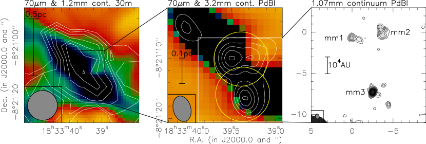
Figure 1: Compilation of the continuum images in IRDC 18310-4 (Beuther et al., 2013, 2015). The left and middle panels show in color the Herschel 70 $\mu$m image with a stretch going dark for low values. The white contours in the left panel show the 1.2 mm MAMBO continuum observations starting from 4$\sigma$ and continuing in 1$\sigma$ steps with a $1\sigma$ value of 13 mJy beam^-1. The contours in the middle panel presents the 3.2 mm PdBI continuum data starting from 3$\sigma$ and continuing in 2$\sigma$ steps with a $1\sigma$ value of 0.08 mJy beam^-1. The two yellow circles outline the $\sim$9^′′ inner third of the two pointings (field 1 north, field 2 south) we observed in this polarization project. The right panel then shows the new 1.07 mm ALMA continuum observations starting from 3$\sigma$ and continuing in 1$\sigma$ steps with a $1\sigma$ value of 0.6 mJy beam^-1.

The Atacama Large Millimeter Array (ALMA) with its polarization capabilities now allows us to address the magnetic field aspect observationally in depth. To investigate the magnetic field properties at the onset of high-mass star formation, we selected the infrared dark cloud IRDC18310-4 located at an approximate distance of 4.9 kpc (Sridharan et al., 2005). The region is infrared dark even at 70 $\mu$m wavelengths, has a mass reservoir of $\sim$800 M_⊙ within roughly a square parsec, and shows no signs of active star formation (Fig. 1 shows a compilation of previous data). The region was studied with the Plateau de Bure Interferometer in the 3 mm and 1 mm band, and hierarchical fragmentation on increasingly smaller scales down to $\sim 2500$ AU was identified (Beuther et al., 2015). Spectral line signatures indicate that the whole maternal gas is likely globally collapsing, fragmenting and at the onset of star formation (Beuther et al., 2013, 2015). The fragment separations in that region are consistent with thermal Jeans fragmentation, however, the core masses are more than an order of magnitude larger than the typical Jeans mass (Beuther et al., 2015). They suggest that this discrepancies can be reconciled by invoking either non-homogeneous initial density structures or strong magnetic fields. Here, we are investigating the magnetic field properties of the region.

2 Observations

The infrared dark cloud IRDC18310-4 was observed with the Atacama Large Millimeter Array (ALMA) as a cycle 3 project (2015.1.00492.S) during four sessions between June 17 and June 20, 2016. The observations were conducted in the 1 mm band with the at that time for ALMA polarization observations still predefined frequency setting with the LO at 233 GHz to avoid any strong line contamination. The four basebands with 2 GHz bandwidth each were centered at 224, 226, 240 and 242 GHz. The channel width was 31.25 MHz. At this frequency, the primary beam of the ALMA 12 m array is $27^{\prime\prime}$, in principle large enough to encompass our region of interest. However, taking into account that ALMA still recommends that only the inner third of the primary beam is reliable for polarization measurements, we used two fields centered on the main continuum sources as shown in Fig. 1. The two corresponding phase centers are for field 1 R.A. (J2000.0) 18:33:39.4, Dec. (J2000.0) -08:21:10.2 and for field 2 R.A. (J2000.0) 18:33:39.4, Dec. (J2000.0) -08:21:16.0, separated by only $5.8^{\prime\prime}$ in declination. Two slightly different array configurations were used (C36-2, C36-3) with a total baseline range between 15 and 704 m. The shortest baseline would correspond theoretically to maximum recoverable scales of approximately $22^{\prime\prime}$. However, typically such theoretical limits are not achieved in interferometric imaging because of the weighting of data and missing baselines also at intermediate scales. ALMA reports for the given configurations maximum recoverable scales of $\sim$11^′′ at 230 GHz. Hence, large-scale flux is still filtered out which will be quantified in the coming section. Eight executions (two per session) of the same scheduling block were conducted with on average 35 good antennas in the array. The execution times per scheduling block varied between 85 and 99 min, and the on-source integration time for each observed field was $\sim$17.6 min per execution. Bandpass calibration was conducted with observations of the quasar J1751+0939 whereas the absolute flux was calibrated with J1733-1304 or Titan. The absolute flux uncertainty should be around 10%. To calibrate phases and amplitudes, regularly interleaved observations of the quasar J1912-0804 were used. The polarization calibration was conducted with J1743-0350.

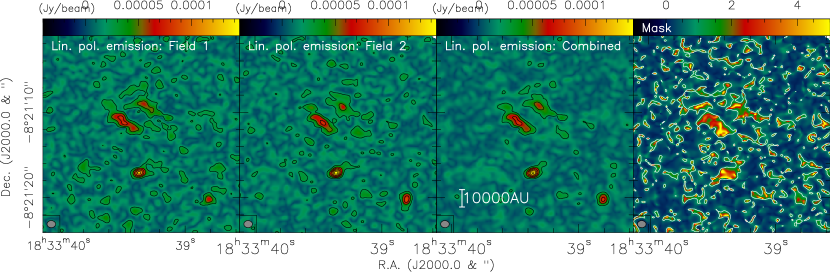
Figure 2: Comparison of the individually and combined two fields. The left panel shows the linearly polarized emission using only field 1, the second panel presents the same for using only field 2, and the third panel shows the combined image. The contour levels are always chosen as the 4$\sigma$ levels of the combined image where 1$\sigma$ is 6 $\mu$Jy beam^-1. The right panel presents the mask created from the combined image and the residuals of each individual image following Matthews et al. (2014), see section 2. The contour level is set to 1, corresponding to the $3\sigma$ confidence level in Matthews et al. (2014). The beam sizes are shown at the bottom-left of each panel, and the combined image also shows a scale bar.

Calibration and imaging of the data was done in CASA version 4.7. For the calibration we followed the provided procedures from the ALMA observatory. Because the two target fields are so closely spaced, we want to combine them in a single image. However, since the main sub-structures are partly outside the recommended inner third of the primary beam (Fig. 1), tests of the individually imaged fields and combined images were conducted. Figure 2 shows the linearly polarized images of the region for each of the two fields separately as well as for the combined dataset. The structures between the two individually imaged fields agree well, and the combined image has the expected lower rms. We conducted an additional test following the approach outlined in Matthews et al. (2014) where the residuals of the linearly polarized Q and U components ($Q_{\rm{res}}$ & and $U_{\rm{res}}$) are calculated first. Then the combined image ($\sqrt{Q^{2}+U^{2}}$) is compared to the residual image to gauge the trustworthiness of the combination. In practice we calculated

$$Q_{\rm{res}}=(Q_{1}-Q_{2})/2\hskip 8.5359pt\&\hskip 8.5359ptU_{\rm{res}}=(U_{1}-U_{2})/2$$ (1)

$$Mask=\frac{\sqrt{Q^{2}+U^{2}}}{3\times\sqrt{Q^{2}_{\rm{res}}+U^{2}_{\rm{res}}}}$$ (2)

In equation 2, the mask is created for the combined linear polarized image, which is above three times the combined residual image. The corresponding mask-image is shown in the right panel of Fig. 2. Clearly, the main structures in the polarized intensity map are several times above the here calculated $3\sigma$ value, showing again that the combination of the two fields is a valid approach.

Based on these tests, we imaged both datasets together in a mosaic mode with natural weighting and a small uv-taper on the longer baselines to increase our signal-to-noise ratio. All four spectral windows were used for the imaging process. The synthesized beam of these images is $1.01^{\prime\prime}\times 0.83^{\prime\prime}$ (PA 89^o). The $1\sigma$ rms values of the Stokes I and the linear polarized image are 0.15 mJy beam^-1 and 6 $\mu$Jy beam^-1, respectively.

3 Results

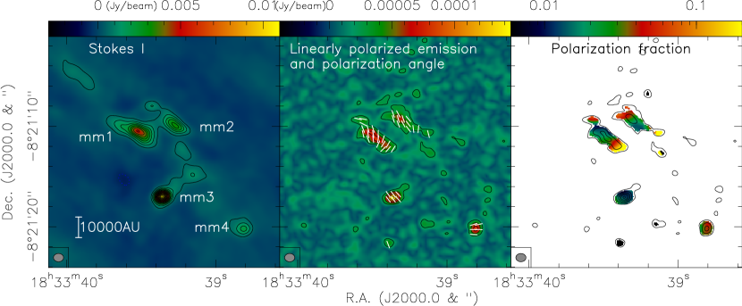
Figure 3: Polarization data at 1.3 mm wavelength for IRDC18310-4. The left panel shows the Stokes I emission ($4\sigma$ contours of 0.6 mJy beam^-1), and the middle panel presents the linearly polarized emission ($4\sigma$ contours of 24 $\mu$Jy beam^-1). The line segments show the corresponding polarization angles (the magnetic field should be rotated by 90 ^∘). The right panel shows for comparison the polarization fraction in color with the same contours of linearly polarized emission as in the middle panel. The polarization fraction should be considered as upper limit because Stokes I may be more strongly affected by interferometric spatial filtering than the weaker polarized emission.

The following analysis is based on the combined dataset of both observed fields. Fig. 3 presents an overview of the obtained data. The left panel shows the Stokes I image of the region, and we clearly re-identify the three main continuum peaks known from the previous PdBI observations (Fig. 1). In addition to these main sources, the more sensitive ALMA data identify additional dust continuum sources in the field. Particularly strong is the south-western source mm4, whereas some weaker features are found between mm2 and mm3 as well as at the north-eastern edge of the field. We will concentrate the study of the linearly polarized emission on the four strongest sources mm1 to mm4. The peak ($S_{\rm{peak}}$) and integrated fluxes ($S_{\rm{int}}$) within the $4\sigma$ contours are shown in Table 1. The total integrated flux density of the whole region is recovered in the Stokes I image of Fig. 3 is 72 mJy beam^-1. For comparison the single-dish 1.2 mm bolometer flux density measured with the MAMBO camera at the IRAM 30 m telescope (Beuther et al., 2002) within the inner $11^{\prime\prime}$ beam size is 132 mJy, and the 1.2 mm single-dish MAMBO flux density measured within the ALMA primary beam area is $\sim$410 mJy. Taking into account that there is a slight difference in the observed wavelength between the 1.2 mm single-dish and the 1.3 mm of the ALMA data approximately 20-50% of the total flux are recovered by our interferometer observations. Assuming optically thin dust emission and following the approach already used in Beuther et al. (2013, 2015) we can calculate the H₂ column densities (N${}_{\rm{H}_{2}}$) and gas masses for the four sub-regions. With gas temperatures in this starless core around $\sim$15 K, a gas-to-dust mass ratio of 150 (Draine, 2011), and a dust opacity index $\kappa$ discussed in Ossenkopf & Henning (1994) for grains with thin ice mantles at densities of $10^{6}$ cm^-3 ($\kappa_{1.3\rm{mm}}\sim 0.9$ cm²g^-1), the derived column densities and masses are presented in Table 1. With the main uncertainties in the dust model and the temperature, we estimate the accuracy of the masses and column densities within a factor 2. The core masses range between roughly 4 and 22 M_⊙ and the H₂ column densities between $2.4\times 10^{23}$ and $1.36\times 10^{24}$ cm^-2, consistent with the previous findings in Beuther et al. (2015).

Table 1: Source parameters

	$S_{\rm{peak}}$	$S_{\rm{int}}$	N${}_{\rm{H}_{2}}$	$M$
	$\left(\frac{\rm{mJy}}{\rm{beam}}\right)$	(mJy)	($10^{23}$cm-2)	(M⊙)
mm1	4.9	19.4	5.7	22.4
mm2	3.2	8.3	3.8	9.6
mm3	1.2	14.4	13.6	16.7
mm4	2.1	3.9	2.4	4.5

In the context of the magnetic field investigation even more important, Fig. 3 presents in the middle panel the linearly polarized emission from the region. All four main mm continuum sources are clearly detected in the polarized emission. Fig. 3 also presents the observed polarization angles, and within each of the four cores, the polarization angles exhibit a relatively ordered structure. While for the more compact sources mm3 and mm4 less independent polarization angle measurements are possible, the orientation in the two sources is roughly in northeast-southwest and east-west directions for the two regions, respectively. For the more extended sources mm1 and mm2, the polarization angle distribution shows some smooth angle shifts over the extents of the structures. The well-structured polarization angles are already a first indication that the magnetic field may be important in that region because turbulence-dominated regions would show less structured polarization angle distributions. We also do not see signs of polarization holes toward the peak positions like those observed previously toward low-mass star-forming regions (e.g., Wolf et al. 2003; Hull et al. 2014). However, that fact that the mean polarization angles toward the four main mm sources are very different may be one explanation for the sometimes observed polarization holes in single-dish data (e.g., Matthews et al. 2009). Single-dish observations would average over the polarization properties of the four sub-sources which could result in a lowered signal toward the lower-resolution single-dish data. In addition to this, the right panel in Fig. 3 presents the corresponding polarization fraction, and we find values typically between 1 and 10%. The latter high values should be considered as upper limits because the much stronger Stokes I emission, that may come from comparably larger scales, may be more strongly affected by interferometric spatial filtering than the weaker polarized emission. While we can measure the missing flux for Stokes I (see above), we do not have the single-dish information for the linearly polarized emission. Hence, we cannot conclusively answer how much missing flux differences between polarized and non-polarized emission may affect the polarization fraction measurement. For comparison, Hull et al. (2014) measured in their TADPOL magnetic field study of 30 mainly low-mass star-forming regions (with a few high-mass more evolved regions included) typical polarization fractions between 1 and $\sim$8%, largely consistent with our measurement. However, they also find at $2.5^{\prime\prime}$ regularly polarization holes toward the peak positions which is not evident in our data. This indicates that at the scales resolved here for IRDC 18310-4, the magnetic field structure is still largely ordered and coherent.

4 Magnetic fields

4.1 Magnetic field strength via Davis-Chandrasekhar-Fermi method

The Davis-Chandrasekhar-Fermi method (hereafter the DCF, Davis, 1951; Chandrasekhar & Fermi, 1953) can be used to calculate the magnetic field strength in a gas if the angular dispersion of the local magnetic field orientations $\sigma_{\psi}$, the gas density $\rho$, and the one dimensional velocity dispersion of the gas $\sigma_{v}$, are known. Assuming that the magnetic field is frozen into the gas and that the dispersion of the local magnetic field orientation angles is due to transverse and incompressible Alfvén waves, then the strength of the plane-of-the-sky component of the magnetic field is

$$B^{\rm{DCF}}_{\perp}=\sqrt{4\pi\rho}\frac{\sigma_{v}}{\sigma_{\psi}}.$$ (3)

We calculate $B^{\rm{DCF}}_{\perp}$ using the procedure described in appendix D of Planck Collaboration et al. (2016a). We estimate $\rho$ assuming an average number density $n=10^{6}$ cm^-3 (Beuther et al., 2013) and a mean molecular weight $\mu=2.8\,m_{p}$, where $m_{p}$ is the proton mass. The one-dimensional velocity dispersion $\sigma_{v}$ is estimated from the width of the N₂H⁺ line measured in this region (Beuther et al., 2015). With a line width $\Delta v(\rm{N_{2}H^{+}})\sim 0.3$ km s^-1, we get $\sigma_{v}\approx\Delta v(\rm{N_{2}H^{+}})/\sqrt{8\rm{ln}2}\approx 0.3\rm{km/s}/\sqrt{8\rm{ln}2}\approx 0.13$ km s^-1. Because more accurate, individual estimates per core are difficult, we use the same value of $\sigma_{v}$ and $n$ for all three sub-regions. We estimate the values of the angular dispersion of the local magnetic field orientations directly from the Stokes $Q$ and $U$ by using

$$\sigma_{\psi}=\sqrt{\left<(\Delta\psi)^{2}\right>},$$ (4)

where

$$\Delta\psi=0.5\times\arctan\left(\frac{Q\left<U\right>-\left<Q\right>U}{Q\left<Q\right>-\left<U\right>U}\right)$$ (5)

and $\left<\cdots\right>$ denotes an average over the selected pixels in each map. The angular dispersions of the polarization vectors as well as the derived magnetic field values are presented in Table 2 for mm1 to mm3 (mm4 is too close to a point source for reasonable estimates). On average we find comparably high magnetic field values in the several hundred $\mu$G to mG regime.

The formal errors are calculated from the $4\sigma$ rms values from the individual Stokes Q and U maps and the area of the calculations. The error for mm3 is largest because it is the smallest source and hence dominated by beam effects. One should keep in mind that the absolute errors for the Davis-Chandrasekhar-Fermi method are even larger because of its underlying assumptions and the effect of projection and line-of-sight integration, which are discussed in detail in appendix D of Planck Collaboration et al. (2016b). For example, it is difficult to determine whether the measured dispersion around the mean field $\sigma_{\psi}$ is exclusively the effect of magneto-hydrodynamic waves and turbulence. Moreover, the observed value of $\sigma_{\psi}$ is an average of various magnetic field vectors, and integration of multiple components along the line may decrease the measurable polarization angle compared to the true dispersion of the magnetic field orientation. Furthermore, the velocity dispersion estimates are obtained using a tracer that does not necessarily sample the same volume as traced by the dust polarization. Finally, the mean densities are assumed whereas density gradients exist within each region. In summary, the magnetic field estimates from the Davis-Chandrasekhar-Fermi method should be considered as order-of-magnitude estimates, which are illustrative of the differences between the regions, but do not fully encompass the complexity of the field dynamics in each one of them.

Table 2: Magnetic field strength estimates

Source	$\sigma_{\psi}$	$B^{\rm{DCF}}_{\perp}$	$b(0)$	$B^{\sc SF}_{\perp}$
	[deg]	[mG]	[deg]	[mG]
mm1	23.1	0.3$\pm$0.1	1.6	3.7$\pm$1.3
mm2	9.8	0.6$\pm$0.2	8.8	0.6$\pm$0.2
mm3	4.3	1.3$\pm$0.4	3.3	1.7$\pm$0.6

4.2 Structure function of the polarization orientation angles

In dense clouds, the magnetic field structure is the result of multiple physical processes not accounted for by the basic DCF analysis. Consequently, dispersion measured about mean fields, assumed straight, may be much larger than should be attributed to magneto-hydrodynamical waves or turbulence. In the region IRDC 18310-4, the distribution of polarization orientation angles, illustrated in Fig. 4, shows that in the sources mm1 and mm2 there is broad distribution or two separate components of polarization orientations, which could lead to an overestimation of $\sigma_{\psi}$ and, correspondingly, an underestimation of $B^{\sc DCF}_{\perp}$.

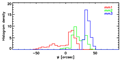
Figure 4: Histogram of polarization orientation angles, $\psi$, towards each of the sources.

Following Hildebrand et al. (2009) and Houde et al. (2009, 2011), we can analyze the structure function (of second order) $S_{2}(\ell)$, also known as the dispersion function, of the polarization angles. This structure function essentially measures the differences between polarization angles separated by displacements $\ell$. Large values in $S_{2}$ reflect large variations whereas small values indicate less dispersion between measured polarization angles. This structure function of the polarization orientation angles $S_{2}(\ell)$ allows for the evaluation of the dispersion of polarization angles, $\sigma_{\psi}$, while avoiding the effect of large-scale non-turbulent perturbations (Hildebrand et al., 2009). The evaluation of $\sigma_{\psi}$ is made by fitting the square of the structure function of polarization angles, $S_{2}(\ell)$, with a second-order polynomial, $S^{2}_{2}(\ell)=b(\ell)+a^{\prime}_{2}\ell^{2}$ above length scales that are dominated by the beam, in this case we chose to fit for $\ell>0.5^{\prime\prime}$. Evaluating the intercept $b(0)$ of that fit gives an alternative measure for the dispersion of polarization angles.

It is evident from the values of $S_{2}(\ell)$, presented in Fig. 5, that the three sources have very different behaviors. In the case of source mm3, the available data does not allow to extend the study of $S_{2}(\ell)$ to $\ell$-values larger than the size of synthesized beam, thus it seems to be dominated by the interferometer resolution. In the case of source mm2, the values of $S_{2}(\ell)$ lead to a value of $b(0)$ that is very close to the values of $\sigma_{\psi}$ estimated using Eq. 4, suggesting that despite the two peaks in the orientation angle distribution the assumption of a single straight mean magnetic field direction is not too inadequate for this region.

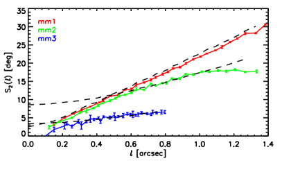
Figure 5: Structure function of the polarization orientation angles, $S_{2}(\ell)$, towards each of the sources. The dashed lines correspond to the fit to the values of $S_{2}(\ell)$ in the range $\ell>0.5^{\prime\prime}$.

The case of source mm1 is, however, very different from the that of mm2 and mm3. There, the relatively large values of $\sigma_{\psi}$ reflects the broad orientation angle distribution, but in contrast to mm2, the values $S_{2}(\ell)$ of the dispersion of polarization orientation angles that can be directly attributed to turbulence is very small, that is, $b(0)=$1.6 deg. This indicates that in mm1 the mean magnetic field direction is not straight and that despite the conclusions that can be drawn from the simple DCF, the magnetic field has to be comparatively stronger. The values of the magnetic field 5strengths based on the angle dispersions calculated from $S_{2}(\ell)$, $B^{\sc SF}_{\perp}$ are also summarized in Table 2.

4.3 Magnetic field implications

With an approximate mean magnetic field strength in the plane of the sky of 2.0 mG ($B^{\sc SF}_{\perp}$ values in Table 2) and a typical density of $10^{6}$ cm^-3 (Beuther et al., 2013), the one-dimensional Alfven velocity is $\sigma_{A}=B/\sqrt{4\pi\rho}\sim 2.6$ km s^-1. In the following we assume that the one-dimensional Alfven velocity in the plane of the sky is the same as that along the line of sight. For comparison, the one-dimensional velocity dispersion for individual cores is $\sigma_{v}\sim$0.13 km s^-1 (see above, Beuther et al. 2015). Or using the approximate line width of the whole maternal clump of $\Delta v\sim 1.5$ km s^-1 (Beuther et al., 2013), the corresponding one-dimensional velocity dispersion is $\sim$0.64 km s^-1. These numbers indicate that any turbulent or infall velocity is below the Alfvenic velocity. Following Girart et al. (2009) or Beuther et al. (2010), we can estimate the ratio of turbulent-to-magnetic energy as $\beta\sim 3(\sigma_{v}/\sigma_{A})^{2}$. Using the larger line-of-sight velocity dispersion of the whole clump that results in turbulent-to-magnetic energy ratio of $\beta\approx 0.18$ whereas the lower $\sigma_{v}$ for the individual cores would result in $\beta\approx 0.008$. Hence, for this high-mass starless region, the magnetic energy appears to dominate over the turbulent energy and thus should be an important ingredient for the formation of high-mass stars.

In our previous study of the region (Beuther et al., 2015), we discussed whether thermal Jeans fragmentation can explain the general fragmentation properties of the region or whether an adapted turbulent Jeans fragmentation may be more likely. While the fragment separations were found to be consistent with thermal Jeans fragmentation, the fragment masses are much higher than the thermal predictions (Beuther et al., 2015). Although turbulent Jeans fragmentation could explain the higher masses, the fact that the measured line width toward individual cores are so small (Beuther et al., 2015) does make the turbulent interpretation less likely. In that context, it is interesting to investigate how the magnetic field would affect such estimates. If one replaces the thermal sound speed at the given low temperatures of $\sim$15 K by the Alfven velocity estimated above, the estimated length scales would rise by up to a factor 20, and the estimated masses by even the cube of that. Such high separations and masses exceed the observed values (Beuther et al., 2015). Hence, while the magnetic field definitely influences the fragmentation of the region, such a simplified “magnetic Jeans fragmentation” picture cannot explain the observed data alone.

A different way to gauge the stability of a region is the mass-to-flux ratio $M/\Phi_{B}\approx 7.6\times 10^{-24}\frac{N_{\rm{H_{2}}}}{B}$ that is given in units of the critical mass-to-flux ratio $(M/\Phi_{B})_{\rm{crit}}$ (with $N_{\rm{H_{2}}}$ and $B$ in cm^-2 and mG; Crutcher 1999; Troland & Crutcher 2008). Using the average magnetic field of $\sim$2.0 mG and the column density $N_{\rm{H_{2}}}\sim 1.3\times 10^{23}$ cm^-2 observed on larger-scales ($11^{\prime\prime}$) with single-dish instruments (Beuther et al., 2013), we get a mass-to-flux ratio $M/\Phi_{B}$ of $\sim$0.5. This is likely a lower limit because it may well be that the magnetic field strength on larger spatial scales could be lower than what we measure at the higher inner densities. Using the higher average column densities from these ALMA observations $N_{\rm{H_{2},av}}\sim 8.2\times 10^{23}$ cm^-2, one gets $M/\Phi_{B}\sim 3.1$. This indicates that while on large scales the overall gas clump may still be at the verge of criticality, on smaller scales it should be collapsing. Such early collapse motions are also inferred from the spectral line data in Beuther et al. (2015).

5 Discussion and conclusions

To the authors knowledge, this is the first high-spatial-resolution magnetic field study of a very young high-mass star-forming region at the onset of collapse prior to any signpost of star formation. For more evolved regions hosting high-mass protostellar objects and/or hot molecular cores, the findings about the importance of the magnetic field are ambiguous. While for some regions the magnetic field should play a dominant role (e.g., G31.4, W75N, W51 or CepA; Girart et al. 2009; Surcis et al. 2009; Tang et al. 2009; Vlemmings et al. 2010), other systems appear to be more strongly influenced by dynamic motions (e.g., IRAS 1809-1732; Beuther et al. 2010). The magnetic field values estimated for IRDC 18310-4 on the order of $\sim$2 mG are lower than what is found for several more evolved hot-core like regions, e.g., W3(H₂O), IRAS 18089-1732 or NGC7538IRS1 with reported values of 17, 11 and 2.5 mG, respectively (Chen et al., 2012; Beuther et al., 2010; Frau et al., 2014). With only one high-mass starless region observed so far, this difference is not conclusive yet, but it will be interesting to see with future data whether the measured magnetic field strengths are indeed related to the evolutionary stage.

Our finding for this high-mass starless region that the mass-to-flux ratio is of order unity (depending on the column density) and at the same time the turbulent-to-magnetic energy ratio is comparably low are both indications for the general instability of the region. The latter fact mainly implies that turbulence is not contributing significantly to the stability of the region. But stability is not needed anyway, because the kinematic signatures found by Beuther et al. (2015) already implied that the whole gas clump is globally collapsing and at the verge of star formation. This is consistent with the high mass-to-flux ratio. The mean magnetic field strength around $\sim$2.0 mG does not contradict that picture, it just implies that the magnetic field significantly contributes to the fragmentation and collapse properties of the overall gas clump. For example, high magnetic field values can inhibit fragmentation into many low-mass cores (e.g., Commerçon et al. 2011; Peters et al. 2011; Myers et al. 2013, 2014; Fontani et al. 2016). For IRDC 18310-4, even at the higher resolution of the previous PdBI observations, several of the cores do not fragment but show masses in excess of 10 M_⊙ (Beuther et al., 2015). Although the sensitivity of these data is not sufficient to detect cores below 1 M_⊙, the fact that massive non-fragmenting cores at the given spatial resolution are identified, is indicative of large magnetic fields that we observe now with the new ALMA data. The overall smooth spatial structure of the polarization angles is additional evidence for the dynamic importance of the magnetic field.

In summary, while the maternal gas clump is collapsing at large, the polarization data reveal that the magnetic field is important for the fragmentation and star formation process in this region. However, a single case study is not sufficient for a general conclusion, and it can only set the stage for future studies of larger samples.