Inference, Learning and Attention Mechanisms that Exploit and Preserve Sparsity in CNNs

Abstract

Convolutional neural networks (CNNs) are a powerful tool for pattern recognition and computer vision, but they do not scale well to higher-dimensional inputs, because of the associated memory demands for storing and manipulating high-dimensional tensors. This work starts from the observation that higher-dimensional data, like for example 3D voxel volumes, are sparsely populated. CNNs naturally lend themselves to densely sampled data, and sophisticated, massively parallel implementations are available. On the contrary, existing frameworks by and large lack the ability to efficiently process sparse data. Here, we introduce a suite of tools that exploit sparsity in both the feature maps and the filter weights of a CNN, and thereby allow for significantly lower memory footprints and computation times than the conventional dense framework, when processing data with a high degree of sparsity. Our scheme provides (i) an efficient GPU implementation of a convolution layer based on direct, sparse convolution, as well as sparse implementations of the ReLU and $max$-pooling layers; (ii) a filter step within the convolution layer, which we call attention, that prevents fill-in, i.e., the tendency of convolution to rapidly decrease sparsity, and guarantees an upper bound on the computational resources; and (iii) an adaptation of back-propagation that makes it possible to combine our approach with standard learning frameworks, while still benefitting from sparsity in the data as well as the model.

1 Introduction

Deep convolutional neural networks (CNNs) are nowadays the state-of-the-art tool for a wide spectrum of computer vision task (Krizhevsky et al.,, 2012; Long et al.,, 2015; Ren et al.,, 2015). A main reason for their spectacular comeback, perhaps even the single most important factor, is that today the necessary computer hardware is available to train and apply deep neural networks with millions of tunable parameters. Graphics Processing Units (GPUs) have brought about an enormous speed-up for massively parallel computation tasks. In particular, this includes both the training (error back-propagation) and inference (forward pass) steps of neural networks, where both the response maps (feature maps) within the network and the network parameters (filter weights) form regular grids that are conveniently stored and processed as tensors.

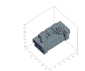
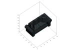
However, while naturally suited for image processing, regular grids are not an ideal representation for sparse data such as line drawings or irregular 3D point clouds (Fig. 1). E.g., the latter are typically acquired with line-of-sight instruments, thus the large majority of points lies on a small number of $2$D surfaces. When represented as occupancies in a 3D voxel grid, they therefore exhibit a high degree of sparsity, as most voxels are empty; while at the same time 3D data processing with CNNs is challenged by high memory demands (Brock et al.,, 2017; Wu et al.,, 2015; Maturana and Scherer,, 2015; Huang and You,, 2016).

$\;\;\;\;r=16$	$\;\;\;\;r=32$
$\;\;\;\;\overline{\rho}=15.5\%$	$\;\;\;\;\overline{\rho}=9.1\%$
$\;\;\;\;r=64$	$\;\;\;\;r=128$
$\;\;\;\;\overline{\rho}=5.3\%$	$\;\;\;\;\overline{\rho}=2.7\%$

Figure 1: Sparsity of volumtric 3D data representations. The density $\overline{\rho}$ of occupied voxels is low for 3D models from Modelnet40, and decreases with growing voxel resolution $r^{3}$.

Figure 2: With suitable computational mechanisms, sparsity in the input can be preserved throughout the CNN. Shown are the activations for one channel of the 1${}^{\text{st}}$, 2${}^{\text{nd}}$ and 3${}^{\text{rd}}$ convolution layers on MNIST for a dense network (top) and for a sparse network with the fraction of non-zero elements restricted to at most $\rho_{up}=15\%$ (bottom).

A conceptually straight-forward counter-measure is to make explicit the sparsity of the feature maps and store them in a sparse data format, see Fig. 2. Moreover, it can be beneficial to also represent the CNN parameters in a sparse manner to improve runtime and – perhaps more important with modern, deep architectures – memory footprint; especially if the sparsity is promoted already during training through appropriate regularisation.

In a sufficiently sparse setting, a significant speed-up can be achieved if one performs convolution directly, incrementally updating a layer’s output map only where there are non-zero entries in the input map as well as non-zero filter weights. This has recently been confirmed independently by two concurrent works (Engelcke et al.,, 2016; Park et al.,, 2017). Computing convolution directly guarantees that only the minimal necessary amount of operations is carried out. However, performing selective updates only at indexed locations makes parallelisation harder. This may be the reason why, to our knowledge, no practical implementations with sparse feature maps exist. In this work we develop a framework to exploit both sparse feature maps and sparse filter parameters in CNNs. To that end

1. we provide sparse versions of the fundamental building blocks of CNNs, namely a sparse Direct Convolution Layer, as well as sparse ReLU and max-pooling layers;

2. we extend the back-propagation algorithm to preserve sparsity, and make our sparse layers usable with existing optimisation routines that are employed in modern deep learning frameworks designed for dense data;

3. we propose to add a density-dependent regulariser that encourages sparsity of the feature maps, and a pruning step that suppresses small filter weights. This regularisation guarantees that the network gets progressively faster at its task, as it receives more training.

All these steps have been implemented on GPU (and also on CPU) as extensions of Tensorflow, for generic $n$-dimensional tensors. The source code is available at https://github.com/TimoHackel/ILA-SCNN. In a series of experiments, we show that it outperforms its dense counterpart in terms of both runtime and memory footprint when processing sparse data, and makes it possible to process 3D data at higher voxel resolutions.

The present paper is based on the preliminary version (Hackel et al.,, 2018).

2 Related work

2.1 Dense CNN for sparse data

Neural networks offer the possibility to learn a mapping from input data to a desired output end-to-end, completely avoiding heuristic feature design and feature selection. Deep, convolutional neural networks are at present the method of choice for a wide range of 2D image interpretation tasks, including object recognition (He et al.,, 2016) and detection (Ren et al.,, 2015), semantic segmentation (Chen et al.,, 2018), motion (Ilg et al.,, 2017) and depth estimation (Zhou et al.,, 2017), and many others. Moreover, deep learning has been adapted to 3D voxel grids (Prokhorov,, 2010; Lai et al.,, 2014; Maturana and Scherer,, 2015; Wu et al.,, 2015), RGB-D images (Song and Xiao,, 2016) and video (Karpathy et al.,, 2014). Being completely data-driven, these techniques have the ability to capture appearance as well as geometric object properties. Their multi-layered, hierarchical architecture is able to capture and encode a large amount of contextual information. A serious drawback of the straight-forward generalisation to 3D is that operating on (dense) voxel grids derived from (originally sparse) point clouds generates a the huge memory overhead for encoding large contiguous volumes of empty space Moreover, also computational complexity grows cubically with voxel grid resolution, but in fact the data is concentrated on few object surfaces.

2.2 Data sparsity

Therefore, more recent 3D-CNNs make use of the sparsity of occupied voxels prevalent in many practical 3D datasets. In Graham, (2014) a sparse CNN is introduced, which is however limited to small resolutions (in the paper, up to $80^{3}$) because of the rapidly decreasing sparsity due to repeated convolutions. Another strategy is to resort to an octree representation, where empty space (and potentially also large, geometrically simple object parts) are represented at coarser scales than object details Riegler et al., 2017b ; Tatarchenko et al., (2017). Since the octree partitioning is a function of the object at hand, an important question is how to automatically adapt to new, previously unseen objects at test time. While Riegler et al., 2017b ; Wang et al., (2017) assume that the octree structure of the output is known at test time, Tatarchenko et al., (2017); Riegler et al., 2017a ; Wang et al., (2018) learn to predict the octree structure together with the labels. This makes it possible to solve tasks where 3D geometry must be generated, e.g., fusion of partial 3D reconstructions and shape synthesis by interpolation. In Häne et al., (2017) a coarse-to-fine scheme is used to hierarchically predict the values of small blocks of voxels in an octree. Another strategy is to rely only on a small subset of discriminative points, while neglecting the large majority of less informative ones (Li et al.,, 2016; Qi et al., 2017a, ; Qi et al., 2017b, ). The idea is that the network learns how to select the most informative points and aggregates information into global descriptors of object shape via fully-connected layers. This allows for both shape classification and per-point labeling using only a small subset of points, resulting in significant speed and memory gains. Bilateral convolutional layers (Jampani et al.,, 2016) map the data into permutohedral space, thus also exploiting sparsity in the data, but do not have a mechanism to exploit parameter sparsity. Recently, Graham and van der Maaten, (2017); Graham et al., (2018) advocate the strategy to perform convolutions only on non-zero elements in the feature map and find correspondences with the help of hash tables. Empirically, it works fairly well to limit activations to non-zero elements of the input, although in principle it suppresses information exchange across empty space, thus potentially slowing down and holding back the learning.

2.3 Parameter sparsity

Several works address the situation that the model parameters are sparse. Denil et al., (2013) reduce the network parameters by exploiting low rank matrix factorisation. Liu et al., (2015) exploit the decomposition of matrices to perform efficient convolutions with sparse kernel parameters. Some authors (Jaderberg et al.,, 2014; Denton et al.,, 2014) approximate convolution filters to achieve a faster runtime, moreover it has been proposed to reduce the number of parameters by pruning connections (Han et al.,, 2015) or imposing sparsity in an already trained network (Wen et al.,, 2016).

2.4 Direct convolutions

The works of Park et al., (2017); Engelcke et al., (2016); Parashar et al., (2017) are the most related ones to our approach, in that they also compute convolutions in a direct manner to more efficiently convolve sparse feature maps with sparse filters. While Park et al., (2017) use compressed rows as sparse format for the filter parameters, neither Engelcke et al., (2016) nor Park et al., (2017) uses a sparse format for both filter parameters and feature maps. Parashar et al., (2017) implement sparse convolutions on custom-designed hardware to achieve an energy- and memory-efficient CNN. Even though all three works follow a similar idea, only the latter exploits sparsity in both the parameters and the data, with compressed sparse blocks; but requires dedicated, non-standard hardware. Recently, sparse convolution has been extended to allow for arbitrary kernel shapes by explicitly storing the input indices for each output, thus including sparse kernel weights (Choy et al.,, 2019). Moreover, in very recent work the use of sparsity has been pushed further for the particular case of point clouds: Boulch, (2019); Thomas et al., (2019) evaluate the convolution in continuous space, but only at the input point locations.

3 Method

It is a recurring theme in computer science to speed up computations and reduce memory usage by exploiting sparsity in the processed data. Here, we propose a number of techniques to do the same for the specific case of CNN layers, always keeping in mind the specific architectural requirements and limitations of current GPUs, which are the prevalent hardware used to run neural networks. Throughout, sparse tensors are represented and manipulated in a format similar to Coordinate List. Such a format is available in modern software frameworks for deep learning (for instance, the ”SparseTensor” structure in Tensorflow). Indices of populated voxels in the grid, as well as the corresponding data values, are stored in separate tensors of equal size. To minimise memory overhead, the indices of the form $\{batch,index_{x},index_{y},...,channel\}$ are compressed into unique $1D$ keys and only expanded when needed.

To achieve coalesced memory access, which permits efficient caching, the tensors for feature maps are sorted w.r.t. batches and within each batch w.r.t. channels. Likewise, filter weights are sorted w.r.t. the output channels and within each channel w.r.t. the input channels.

Compared to dense tensors, the sparse representation inevitably adds some overhead. In our implementation we use $64$ bit keys, and $32$ bit depth for feature maps. Consequently, storing a dense feature map (100% density) requires 3$\times$ more memory in the Coordinate List format. For densities $<$33% the sparse representation is more efficient, and at low densities the savings can be very significant, e.g., at density 1% it uses 97% less memory. In this context, we note that even less dramatic savings, say $>$50%, can have important consequences in practice: a main bottleneck of deep neural networks, especially for 3D or even 4D data, is the available on-board memory on the GPU, which limits the batch size during training and inference. Overly small batches slow down or even harm the training – up to the point where training becomes impossible because there is not enough memory to pass a single example through the net.

3.1 Sparse convolution

Our convolutional layer is designed to work with sparse tensors for both feature maps and filter weights. Feature maps are updated incrementally with atomic operations, c.f. Algorithm 1. In that respect it is similar to two concurrent works (Parashar et al.,, 2017; Park et al.,, 2017). Atomic operations are a feature of modern GPUs, designed to be small enough to be thread-safe, without having to use a locking mechanism. The incremental update is unfortunately not a perfect match for the current hardware design, since atomic operations are slightly slower than non-atomics: existing off-the-shelf GPUs do not offer native support for atomic floating point operations in shared memory, although they do for more costly CAS instructions. Nonetheless, incremental updating is significantly faster, because it performs only the minimum number of operations necessary to obtain the convolution result, while avoiding to multiply or add zeros.

Algorithm 1 Direct Sparse Convolution with Attention

1:decompress filter and data indices from $1$D to $k$D

2:for $b\in[0:\,$batch_count$]$ do

3:     for $oc\in[0:\,$out_channel_count$]$ do

4:         initialize dense buffer with $0$

5:         for $ic\in[0:\,$in_channel_count$]$) do

6:              for $\{id,val\}\in$ data($b,ic$) do

7:                  for $\{fid,fval\}\in\,$filter($oc,ic$) do

8:                       compute $uid$ with get_update_id($id,fid$)

9:                       atomically add $val\cdot fval$ to buffer at $uid$                                          

10:         get non-zero entries from buffer

11:         add bias to non-zero entries in buffer

12:         select $k$ largest responses from non-zero entries

13:         compress ids of $k$ largest responses from $k$D to $1$D

14:         write $k$ largest features and ids as sparse output      

The sparse convolution is computed sequentially per output channel and batch, but in parallel across input channels, features and filter weights. Its result is stored in a temporary, dense buffer with batch size and channel depth 1. This buffer increases quadratically for 2D images, cubically for 3D volumes, etc. Still, it is in practice a lot smaller than a dense tensor holding all channels for the entire batch, such that volumes up to $512^{3}$ can be processed on a single commodity graphics card (Nvidia Titan Xp, 12 GB).

3.2 Preserving sparsity with attention

(a)

(b)

(c)

(d)

Figure 3: Fill-in (loss of sparsity) due to convolutions depends on the data distribution. Uniformly distributed data is affected most strongly, e.g., in $3$D every $3\times 3\times 3$ filter will increase the density by a factor of $27$, until data is dense.

Convolution with kernels larger than $(1\times 1)$, by construction, generates fill-in, i.e., it generates an output feature map that is a lot less sparse than the input. See Fig. 3. In the presence of well-spaced sparse structures, like for example the surfaces in a 3D scan, this “smearing out” of the sparse inputs into empty space only has a small influence on the output of the network (see the experiments). But it considerably increases memory consumption and runtime, especially when occurring repeatedly over multiple layers. Intuitively, a stack of convolutional layers “diffuses” information over its cumulative receptive field, but with small convolution kernels even a deep stack cannot bridge large empty regions and capture context across them.

Our goal here is to prevent fill-in and maintain a desired level of sparsity, by dropping small feature responses. To that end, we run a $k$-selection filter (Alabi et al.,, 2012) on each output channel and keep only the $k$ strongest (non-zero) responses. The parameter $k$ controls the sparsity of the convolutional layers. Note, for a given network architecture an upper bound on the number of non-zero entries directly translates to a bound on the memory footprint, and for a given hardware configuration also a bound on the runtime. The $k$-selection can be seen as an approximation of the exact convolution. Small responses are suppressed, but with an adaptive threshold that suppresses only as many values as necessary to uphold the desired degree of sparsity. The selection can be interpreted as a form of attention, in the sense that its aim is to manage a limited pool of computational resources and assign them as needed for the solution of the task.

We have implemented two versions of this simple attention mechanism:

• The first one acts on the raw convolution result, so it prefers large positive responses, making it similar to a rectified linear unit;

• The second one picks the $k$ responses with the largest absolute values, giving preference to responses with large magnitude.

Empirically the first version works better, see Section 4.

The overall time complexity to convolve data of dimension $k$, resolution $s_{d}$ and density $\rho_{d}$, with filters of size $s_{f}$ and density $\rho_{f}$, is

$$O\big{(}(\rho_{d}\cdot\rho_{f}\cdot s_{f}^{k}\cdot c_{in}+log(s_{d}^{k}))\cdot s_{d}^{k}\cdot c_{out}\cdot b\big{)}\;,$$ (1)

with $b$ the number of batches and $c_{in},c_{out}$, the number of input and output channels, respectively.

Algorithm 2 Backpropagation for convolutional layer

1:initialize bp_data with shape(input_values) and $0$

2:initialize bp_filter with shape(filter_weights) and $0$

3:decompress filter and data indices from $1$D to $k$D

4:for $b\in[0:\,$batch_count$]$ do

5:     for $oc\in[0:\,$out_channel_count$]$ do

6:         initialize dense buffer with gradients($b,oc$)

7:         for $ic\in[0:\,$in_channel_count$]$) do

8:              for $\{id,val\}\in$ data($b,ic$) do

9:                  for $\{fid,fval\}\in\,$filter($oc,ic$) do

10:                       compute $uid$ with get_update_id($id,fid$)

11:                       get gradient $g$ from buffer at $uid$

12:                       atomically add $g\cdot fval$ to bp_data at $id$

13:                       atomically add $g\cdot val$ to bp_filter at $fid$                                               

3.3 Pooling layer

Our sparse pooling layer has three straight-forward stages. First, assign features to an output (hyper-)voxel, by dividing the data channels of their index by strides. Second, sort the data w.r.t. voxels, so that responses within the same voxel are clustered together. Third, apply the pooling operator separately to each cluster. The time complexity for this is

$$O\big{(}\rho_{d}\cdot s_{d}^{k}\cdot log(\rho_{d}\cdot s_{d}^{k})\cdot c_{in}\cdot b\big{)}\;.$$ (2)

3.4 Direct sparse backpropagation

Our target for back-propagation is again to avoid carrying out operations that are not needed due to sparsity. Clearly, we must propagate error gradients only to those features which have produced evidence, in the form of non-zero responses during the forward pass.

Yet, the problem of rapid fill-in, already discussed for the forward pass, equally affects the backward pass: back-propagation through a convolution layer is itself a convolution that spreads out non-zero values over a neighbourhood, thus increasing memory demands and runtime. Contrary to the forward pass, it is not advisable to bound the fill-in with $k$-selection, as this could seriously slow down or even impair the training: during back-propagation, large error gradients can flow to zero activations and vanish, whereas smaller gradients flowing towards non-zero activations might be missed due to the selection. Hence, we propose to use a stricter back-propagation, which only propagates errors $L$ to non-zero features $x$ and model parameters $w$:

$$\begin{split}&\frac{\partial L}{\partial x_{i}}=\left\{\begin{array}[]{ll}0&\text{for }x_{i}=0\\ \frac{\partial L}{\partial y}\frac{\partial y}{\partial x_{i}},&\text{else}\end{array}\right.\\ &\frac{\partial L}{\partial w_{i}}=\left\{\begin{array}[]{ll}0&\text{for }w_{i}=0\\ \frac{\partial L}{\partial y}\frac{\partial y}{\partial w_{i}},&\text{else}\end{array}\right.\;.\end{split}$$ (3)

Here, weights are considered equal to zero only if they have been explicitly removed by pruning, so as to avoid suppressing the gradients of weights that pass through $w_{i}\!=\!0$ while changing sign. Note the structural similarity of our approximated back-propagation to back-propagation through any layer with $ReLU$ activation: Conventional back-propagation sets values to zero as a function of the layer output $y_{i}$, whereas our scheme sets them to zero as a function of the input $x_{i}$.

Neglecting zero-elements slightly reduces the efficiency per learning iteration, since not all error gradients are propagated anymore. However, this is offset by several of advantages:

1. The tensors used for back-propagation have fixed size and shape. Therefore, one can work with fixed and known array dimensions, and use optimisation frameworks that have been designed for dense data;

2. By considering only gradients on non-zero elements of the forward pass, back-propagation can be implemented in a clean and transparent manner. E.g.  for convolutional layers one obtains Algorithm 2, which is very similar to Algorithm 1;

3. Once a filter weight has been set to zero, it will remain zero. Below, we will describe how this property can be used to guarantee that the network gets progressively faster at its task as the learning proceeds and it sees more training data.

3.5 Adaptive density regularisation

The $k$-selection filter adds to the computational cost of the overall method, but there is also a computationally more efficient way to reduce the number of non-zero feature responses. Although that trick, described in the following, cannot guarantee a bound on the sparsity, it helps to stay below the bound, such that the more costly $k$-selection often need not be invoked.

The $ReLU$ non-linearity used in most modern CNNs, by definition, truncates negative activations to zero while leaving positive ones unchanged. This means that we can encourage sparsity by lowering the values (not magnitudes) of filter weights and biases. In doing so, more weights will drop below $0$ and will be extinguished by the subsequent $ReLU$.

Going back to the idea of maintaining an optimal, rather than maximal, level of sparsity, one can use the same idea to reduce sparsity when there are fewer non-zero values than would fit into the memory and computation budget. When too many activations drop below $0$, one simply drives the filter parameters up, so that fewer responses are suppressed by the $ReLU$. To achieve the desired effect, we simply add a bias $b$ to the $L_{2}$-regulariser on the weights, so that the regulariser becomes $\sum(w+b)^{2}$. The scalar $b$ is positive when the density $\rho$ is too large, and negative when it is overly small:

$$b=\begin{cases}o+b_{1}\cdot(\rho-\rho_{up})&\text{if }\rho>\rho_{up}\\ &\text{(exceeds available resources)}\\ -b_{2}\cdot(\rho_{up}-\rho)&\text{if }\rho\leq\rho_{up}\\ &\text{(not using all resources)}\end{cases}$$ (4)

with $\rho_{up}$ the upper bound implied by the $k$-selection filter, and $o$, $b_{1}$, $b_{2}\geq 0$ control parameters. The bias is asymmetric and adds an extra penalty $o$ for exceeding the available resources, since that would trigger the $k$-selection filter and cause additional computational load.

3.6 Parameter pruning

As explained above, our training algorithm has the following useful properties: (i) The regulariser encourages small model parameters. (ii) The sparse back-propagation ensures that, once set to zero, model parameters do not reappear in later training steps. Together, these two suggest an easily controllable way to progressively favour sparsity during training, by one-warning-shot pruning of weights: At the end of every training epoch we screen the network for weights $w$ that are very small, $|w_{i}|<\epsilon$. If the magnitude of a weight $w_{i}$ stays low for two consecutive epochs (meaning that it was already close to zero before, and still is after one epoch of training) we conclude that it has little influence on the network output and remove it. We note that a small weight should not be pruned when first detected, without warning shot: it could have a large gradient and just happen to be at its zero-crossing from a large positive to a large negative value (or vice versa) at the end of the epoch. On the contrary, it is less likely to observe a weight exactly at its zero-crossing twice in a row.

Since such a weight, once set to zero, will remain zero due to the proposed sparse back-propagation, every pruning can only reduce the number of non-zero weights. It is therefore guaranteed that the network become sparser, and therefore also faster at the task it is learning, as it sees more training data; until a configuration has been reached that is “optimal” in the sense that all weights have significant magnitude and no further pruning is possible. We note, it is well documented that biological systems get faster at cognitive tasks with longer training (Robertson,, 2007; Nissen and Bullemer,, 1987); but we do not claim that the underlying mechanisms are similar.

4 Evaluation

In this section we evaluate the impact of density upper bounds and regularisation on runtime and classification accuracy. The sparse network structures were implemented into the Tensorflow framework and programmed in C++/CUDA with a python interface. Our experiments were run on PCs with Intel Core i7 7700K processors, 64GB RAM and Titan Xp GPUs. Detailed specifications about the different CNN variants used in the experiments (in both sparse and dense versions) are given in the appendix.

To start with, we use a synthetic dataset of sparse random tensors to evaluate the memory footprint and runtime of our convolutional layer, and to compare it against the dense layers of Tensorflow version 1.4 (compiled with Cuda 9.0 and CuDNN 6.0). We conduct different experiments to evaluate the effects of the sparse network variant on classification accuracy: First, the impact of upper bounds on classification is evaluated by performing a grid search on the upper bound $\rho_{up}$ in the convolutional layers. For this experiment, a thresholded version of the MNIST data set (LeCun et al.,, 1998) is used, as it is small enough to perform grid search in a reasonable amount of time and can be interpreted as sparse data (1D lines in 2D images). Second, the effects of pruning on runtime and classification accuracy are shown using the Modelnet data set (Wu et al.,, 2015), by varying the strength $\lambda$ of the regularisation. Modelnet40 provides 3D CAD models of $40$ different classes. Furthermore, the classification results of different baseline methods are compared on this data set, as well as the more recent ScanNet (Dai et al.,, 2017). We train with $adagrad$ (Duchi et al.,, 2011) with learning rate $0.001$. Convergence (change of loss $<10^{-5}$) takes approximately 100 epochs.

Figure 4: Runtime [s] of a dense convolution layer in Tensorflow and of our sparse convolution layer, for random tensors of different resolutions $r^{3}$. At high resolutions the sparse version is much more efficient.

Resolution	$32^{3}$	$64^{3}$	$128^{3}$	$256^{3}$	$512^{3}$
Dense [GB]	$0.04$	$0.27$	$2.15$	$17.18$	$137.28$
Sparse 32bit [GB]	$2\cdot 10^{-3}$	$8\cdot 10^{-3}$	$0.03$	—	—
Sparse 64bit [GB]	$3\cdot 10^{-3}$	$0.013$	$0.05$	$0.2$	$0.8$
Sparse Temp [GB]	$3\cdot 10^{-4}$	$0.002$	$0.016$	$0.13$	$1.07$

Table 1: Memory consumption of a dense conv layer in Tensorflow and of our sparse conv layer, for different resolutions $r^{3}$, with $\rho_{up}=1/r$, minibatch size $32$ and output depth $8$. At high resolutions the sparse version is much more efficient.

Resolution	$16^{3}$	$32^{3}$	$64^{3}$	$128^{3}$	$256^{3}$
Octnet	$16\text{s}$	$1\text{m}6\text{s}$	$5\text{m}30\text{s}$	$34\text{m}43\text{s}$	—
	$3.83$ MB	$20.49$ MB	$114.23$ MB	$549.28$ MB	—
Sparse	$2\text{m}10\text{s}$	$5\text{m}28\text{s}$	$11\text{m}36\text{s}$	$6\text{m}20\text{s}$	$21\text{m}11\text{s}$
	$11.25$ MB	45 MB	180 MB	720 MB	2880 MB

Table 2: Training time and memory footprint of one epoch on Modelnet40 at different resolutions $r^{3}$, for OctNet and for the corresponding version of our sparse network. In all cases we set $\rho_{up}=1/r$ and use minibatch size 32 for single epoch. At $256^{3}$ Octnet runs out of memory.

4.1 Runtime and Memory Footprint

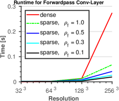
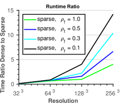
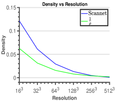
For the evaluation of runtime, convolutions are performed on a sparse voxel grid filled with random numbers. The resolution of the voxel grid $r^{3}$ is varied between $r=16$ and $r=256$. To achieve the expected data density of a $2$D surface in a $3$D voxel grid, the data density $\rho$ as well as the upper bound on the per-channel density $\rho_{up}$ are set to $\rho=\rho_{up}=\frac{1}{r}$. Empirically, the density of real datasets like Scannet is indeed $\approx\frac{1}{r}$ at high resolutions that call for sparse methods. At very low resolution it is a bit higher ($\frac{1.5}{r}$ to $\frac{2}{r}$) due to the presence of multiple surfaces, see Figure 5.

Figure 5: Voxel grid density vs. resolution. At very low resolutions the density is up to $\frac{2}{r}$, but with increasing resolution it quickly decays towards $\frac{1}{r}$, and in fact even falls slightly below that idealised value at resolution $512^{3}$.

To run dense convolution at resolution $r=256$, the mini-batch size and channel depth had to be set to $1$ (Protobuf limits each single tensor to $2$ GB), while the number of output channels was set to $8$. The density $\rho_{f}$ of the filter weights is varied between $0.1$ and $1$. As baseline we use the convolutional layer of standard Tensorflow (Abadi et al.,, 2016), which performs convolutions via the fast Fourier transform and batched general matrix-matrix multiplication from cuBlas, as front end to cuDNN (Chetlur et al.,, 2014). We note that processing only a single input channel does not play to the strength of our sparse network. Moreover, Tensorflow is able to use the full capability of the GPU, while our implementation is limited to operating in global memory, due to the weak support for atomic floating point operations in shared memory. The effect of this limitation is particularly pronounced at small resolution and high density, whereas for high resolutions and low densities its influence fades. In particular, at $r=256$ and $\rho_{f}=0.1$, we are $14\times$ faster with strong density regularisation, so that the $k$-selection step is bypassed; and still $7\times$ faster including $k$-selection filtering. See Figure 4.

Table 1 shows the memory requirements for dense and sparse convolution layers at various resolutions $r$. Dense convolutions require only a single output tensor. The sparse implementation uses tensors for indices and data as well as a temporary buffer, which can be reused in all layers. For the experiment the data type is $32$bit floating point, for the indices we consider both $32$bit and $64$bit. As expected, our sparse representation needs less memory at the sparsity levels of realistic 3D point cloud data. In particular, our sparse version makes it possible to work with large resolutions up to $r=512^{3}$, which is impossible with the dense version on existing hardware. Moreover, we also compare both computation time and memory footprint to Octnet on real Modelnet40 data. Explicit sparsity is approximately on the same level of memory-efficiency, but slower at low resolutions (that can in many cases even be handled with dense voxels). At high resolution it clearly outperforms Octnet. In particular, it still works at resolutions up to $256^{3}$, where Octnet runs out of memory (presumably due to higher peak consumption while building the octree.

4.2 Contribution of small feature responses

In the context of sparsity the question arises, whether zero-valued features contribute valuable information. Two recent works tried to answer this question. On the one hand, Graham and van der Maaten, (2017) found that they reach the same accuracies as dense networks for their application, while completely neglecting zero-valued features. On the other hand, Uhrig et al., (2017) concluded that for certain tasks zero-valued features may be beneficial. In our framework it is possible to assess the importance of small feature responses (not limited to exact zeroes) by training neural networks with varying upper bounds. For this experiment, CNNs are trained on MNIST without regularisation, using the $adagrad$ optimiser and a learning rate of $0.01$. The pixels in MNIST were set to zero when their value $v\in[0,255]$ was below a threshold of $v<50$, to obtain a sparse dataset with average input density $\rho_{in}=0.23$, while the upper bound $\rho_{up}$ ranges from $\rho_{up}=0.035$ to $\rho_{up}=0.075$. Note that even though letters can be interpreted as 1D lines in 2D images, the MNIST data has a low resolution of only $28\times 28$ pixels. Hence, the data is still not very sparse. Results after 10 and after 60 training epochs are given in Table 3. Low upper bounds guarantee a small memory footprint, and also yield slightly faster runtime per epoch. The price to pay is slower convergence, because some gradients are lost during back-propagation; and a slight performance penalty for very strict bounds ($<1\%$ for the strictest setting $\rho_{up}=0.035$).

$\rho_{21}$	$0.035$	$0.05$	$0.075$
Sparse, 10 epochs	$0.954$	$0.971$	$0.976$
Sparse, 60 epochs	$0.985$	$0.990$	$0.992$

Table 3: Influence of small responses. Performance on MNIST with different upper bounds on the density of activation maps.

(a)

(b)

(c)

Figure 6: Influence of adaptive density regularisation and pruning on (left) the number of non-zero filter weights, (middle) the runtime per training epoch, and (right) the accuracy on the Modelnet40 test set. Strong regularisation and pruning save a lot of memory and time without noticeable impact on accuracy.

(a)

(b)

(c)

Figure 7: Performance of sparse net, compared to the equivalent dense net and Octnet on Modelnet40 (left, middle) and ScanNet (right). (left) accuracy for different upper density bounds; (middle, right) accuracy vs. input resolution.

4.3 Regularisation and pruning

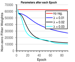
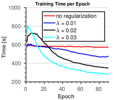
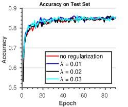
With our sparsity-inducing pruning and regularisation, we expect faster runtime. In order to verify this behaviour, neural networks are trained on Modelnet40 with varying regularisation scales $\lambda\in\{0,0.1,0.2,0.3\}$. The bias for density-based regularisation is computed with $b_{1}=b_{2}=o=0.1$. Stronger regularisation decimates the number of (non-zero) filter weights faster, as shown in Figure 6. It can also be seen that the number of parameters converges when only important weights are left. The drop in non-zero weights also reduces runtime. After $90$ epochs, a network regularised with $\lambda=0.3$ is $51\%$ faster than one trained without regularisation and pruning, even though only the first nine out of twelve convolution layers are set to be sparse. Strong regularisation initially causes an increase in runtime, by driving up the number of non-zero weights to use the available resources via the bias term $b_{2}$. The classification accuracy for all tested regularisation scales quickly converges to practically identical values, as shown in Figure 6. We point out that pruning finds the most suitable sparsity pattern for a given training set. When using a pruned model for transfer learning, it may be safer to re-initialize the removed filter weights of the sparse representation with zeros before fine-tuning.

For completeness, we also empirically compare the two described variants of the $k$-selection filter, where either the $k$ largest signed weights or the $k$ weights with highest magnitude are preserved. See Figure 6. The test, run on Modelnet40, shows that sorting signed weights is preferable, which is not surprising, given the proven performance of the $ReLU$ activation.

Figure 8: Pruning by signed ($RELU$) or unsigned ($ABS$) magnitude. As expected, keeping the largest positive activations, as in the $ReLU$ activation, works better. The experiment was run on Modelnet40 with resolution $16^{3}$.

4.4 Classification performance on Modelnet40

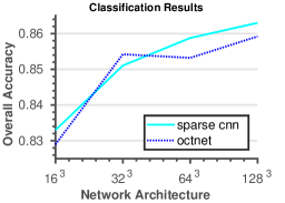
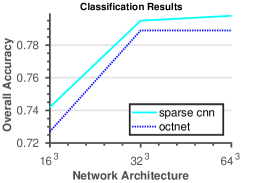
We compare our upper-bounded neural net and modified back-propagation against a conventional dense net. To that end we run the Octnet3 variant of Octnet (Riegler et al., 2017b, ), a dense network without octree structure, and a sparse version of the same network on Modelnet40, see Figure 7.

First, the input resolution is set to $r=16^{3}$, while the upper bound on the density is varied between $\rho_{in}\in\{0.06,0.12,0.33,1.0\}$. Both, the conventional dense network and Octnet converge to a similar overall accuracy of $\approx 0.83$. For a trivial upper bound $\rho_{in}=1.0$ the overall accuracy of our sparse network is also practically the same. Very low upper bounds up to $\rho_{in}=0.12$ yield slightly worse results on the $16^{3}$ inputs, for the lowest bound $\rho_{in}=0.06$ the drop in performance reaches $\approx 3$ percent points. Second, the resolution of the input is gradually increased: $r~{}\in~{}\{16^{3},~{}32^{3},~{}64^{3},~{}128^{3}\}$. Both the sparse network and Octnet yield similar results, for all resolutions. Octnet performs slightly better on $r~{}=~{}32^{3}$, while our bounded, sparse network has a small advantage at all other resolutions. The two experiments suggest that reasonable upper bounds and our sparse backpropagation do not reduce significantly classification accuracy. We have confirmed this further by running experiments at different resolutions, see Figure 7. For these experiments we always use our default density bounds as given in the appendix. The performance of our network closely follows that of Octnet across a range of voxel sizes.

chair	bed	bathtub	floor	desk	curtain
bookshelf	cabinet	counter	door	wall	picture
refrigerator	shower curtain	sink	sofa	table	toilet

Figure 9: Examples from ScanNet, at voxel resolution $64^{3}$. The sparsity is clearly visible for all objects, no matter what their size and shape.

4.5 Classification performance on ScanNet

Additionally, we also test our sparse 3d network on the Scannet dataset. ScanNet provides 3D scans of indoor environments, acquired with a moving RGB-D sensor. In correspondence with the Modelnet experiments, we construct an object classification task, by extracting point clouds of all furniture objects in the dataset, using the ground truth per-point and instance annotations. The ScanNet evaluation uses 19 different classes of furniture (like bathtub, bed, chair, desk,…), plus a rejection class “other furniture”, which we discard for our experiments. Our test thus is a 19-way classification task, where the input are voxel occupancies derived from point clouds that may be incomplete and noisy, but contain only points from the target class. 70% of the dataset are randomly picked as training data, the rest is used for validation. The train/test split remains the same for all evaluated networks. Results are given in Figures 7 and 10. We run experiments with: $r\in\{16,32,64,256\}$. On the highest resolution we did not test the dense CNN, since it is already close to intractable: batch size has to be reduced to 2 even for sparse version, still a single epoch runs for $>11$ hours, which means $>6$ weeks to convergence. The sparse network at resolution $256$ trains more than $10\times$ faster. The performance of our network is almost the same as that of both the equivalent dense network and Octnet (in fact it is slightly better).

Figure 10: Test accuracy for 3d instance classification on Scannet. $\rho$ defines the upper density bound of the first layer, see appendix for detailed specifications. Extreme sparsity does decrease performance a bit, but still gives very reasonable results. Enforcing a moderate amount of sparsity does not seem to hurt the classification. At high resolutions, only sparse networks are tractable.

5 Conclusion

We have proposed novel neural network mechanisms that exploit and encourage sparsity in both feature maps and model parameters. When the input data exhibits a substantial degree of sparsity, our novel sparse layers and back-propagation rule significantly reduce (i) memory footprint and (ii) runtime of convolutional layers at practically useful resolutions. Moreover, our approach guarantees upper bounds on the memory requirements and runtime of the network. For classification tasks the performance of our sparse network is comparable to its dense counterpart, as well as to Octnet. In future work it will be interesting to employ sparsity also for other tasks. Our implementation is fully compatible with Tensorflow and has been released as open-source code. We hope that hardware support for sparse convolutions will improve further on future consumer GPUs, as demonstrated by Parashar et al., (2017); thus further boosting the performance of sparse, high-dimensional CNNs.

Appendix: Network architectures

Table 4 shows the network architectures of our experiments. Depending on the type of data and the goal of the experiment, we used the following network specifications (both for the dense and the sparse version, where applicable):

• For MNIST, we run OctNet3-$24^{2}$ with $10$ output classes. $\rho_{21}$ is set as specified in the paper text and $\rho_{22}=2\cdot\rho_{21}$.

• For Modelnet40 we have $c=40$ different output classes and employ the following variants:

  1. For the regularisation experiment (Figure 6) we use OctNet3-$64^{3}$ with $\rho_{41}=0.06$, $\rho_{42}=0.14$, $\rho_{43}=0.33$.

  2. Figure 7 (left) has been generated with OctNet3-$16^{3}$ with varying upper bounds $\rho_{11}=\{0.06,0.12,0.33,1\}$, $\rho_{12}=\{0.12,0.24,0.33,1\}$.

  3. For Figure 7 (right) the following networks were used: OctNet3-$16^{3}$ with $\rho_{11}=\rho_{12}=1$; OctNet3-$32^{3}$ with $\rho_{31}=0.14$, $\rho_{32}=0.33$, $\rho_{33}=0.66$; OctNet3-$64^{3}$ with $\rho_{41}=0.06$, $\rho_{42}=0.14$, $\rho_{43}=0.33$; OctNet3-$128^{3}$ with $\rho_{51}=0.02$, $\rho_{52}=0.06$, $\rho_{53}=0.14$.

• For ScanNet, we use the same architectures as for Modelnet, but setting the number of output classes to $c=19$.

  1. Figure 7 was generated with OctNet3-$16^{3}$ with $\rho_{11}=0.14$, $\rho_{12}=0.33$; OctNet3-$32^{3}$ with $\rho_{31}=0.14$, $\rho_{32}=0.33$, $\rho_{33}=0.66$; OctNet3-$64^{3}$ with $\rho_{41}=0.06$, $\rho_{42}=0.14$, $\rho_{43}=0.33$.

  2. Figure 10 was generated with:

     1. OctNet3-$16^{3}$ with $\rho_{11}=0.01$, $\rho_{12}=0.03$; OctNet3-$32^{3}$ with $\rho_{31}=0.01$, $\rho_{32}=0.03$, $\rho_{33}=0.03$; OctNet3-$256^{3}$ with $\rho_{61}=0.01$, $\rho_{62}=0.03$, $\rho_{63}=0.07$.

     2. OctNet3-$16^{3}$ with $\rho_{11}=0.03$, $\rho_{12}=0.05$; OctNet3-$32^{3}$ with $\rho_{31}=0.03$, $\rho_{32}=0.05$, $\rho_{33}=0.05$; OctNet3-$256^{3}$ with $\rho_{61}=0.03$, $\rho_{62}=0.05$, $\rho_{63}=0.07$.

     3. OctNet3-$16^{3}$ with $\rho_{11}=0.05$, $\rho_{12}=0.07$; OctNet3-$32^{3}$ with $\rho_{31}=0.05$, $\rho_{32}=0.07$, $\rho_{33}=0.07$; OctNet3-$64^{3}$ with $\rho_{41}=0.05$, $\rho_{42}=0.07$, $\rho_{43}=0.14$.

     4. OctNet3-$16^{3}$ with $\rho_{11}=0.07$, $\rho_{12}=0.09$; OctNet3-$32^{3}$ with $\rho_{31}=0.07$, $\rho_{32}=0.09$, $\rho_{33}=0.09$; OctNet3-$64^{3}$ with $\rho_{41}=0.07$, $\rho_{42}=0.09$, $\rho_{43}=0.18$.

     5. OctNet3-$16^{3}$ with $\rho_{11}=0.14$, $\rho_{12}=0.33$; OctNet3-$32^{3}$ with $\rho_{31}=0.14$, $\rho_{32}=0.33$, $\rho_{33}=0.66$; OctNet3-$64^{3}$ with $\rho_{41}=0.6$, $\rho_{42}=0.14$, $\rho_{43}=0.33$.

OctNet3-$16^{3}$	OctNet3-$24^{2}$	OctNet3-$32^{3}$	OctNet3-$64^{3}$	OctNet3-$128^{3}$	OctNet3-$256^{3}$
conv($1$, $8$, $\rho_{11}$)	conv($1$, $8$, $\rho_{21}$)	conv($1$, $8$, $\rho_{31}$)	conv($1$, $8$, $\rho_{41}$)	conv($1$, $8$, $\rho_{51}$)	conv($1$, $8$, $\rho_{61}$)
conv($8$, $8$, $\rho_{11}$)	conv($8$, $8$, $\rho_{21}$)	conv($8$, $8$, $\rho_{31}$)	conv($8$, $8$, $\rho_{41}$)	conv($8$, $8$, $\rho_{51}$)	conv($8$, $8$, $\rho_{61}$)
conv($8$, $8$, $\rho_{11}$)	conv($8$, $8$, $\rho_{21}$)	conv($8$, $8$, $\rho_{31}$)	conv($8$, $8$, $\rho_{41}$)	conv($8$, $8$, $\rho_{51}$)	conv($8$, $8$, $\rho_{61}$)
maxPooling(2)	maxPooling(2)	maxPooling(2)	maxPooling(2)	maxPooling(2)	maxPooling(2)
conv($8$, $16$, $\rho_{12}$)	conv($8$, $16$, $\rho_{22}$)	conv($8$, $16$, $\rho_{32}$)	conv($8$, $16$, $\rho_{42}$)	conv($8$, $16$, $\rho_{52}$)	conv($8$, $16$, $\rho_{62}$)
conv($16$, $16$, $\rho_{12}$)	conv($16$, $16$, $\rho_{22}$)	conv($16$, $16$, $\rho_{32}$)	conv($16$, $16$, $\rho_{42}$)	conv($16$, $16$, $\rho_{52}$)	conv($16$, $16$, $\rho_{62}$)
conv($16$, $16$, $\rho_{12}$)	conv($16$, $16$, $\rho_{22}$)	conv($16$, $16$, $\rho_{32}$)	conv($16$, $16$, $\rho_{42}$)	conv($16$, $16$, $\rho_{52}$)	conv($16$, $16$, $\rho_{62}$)
sparseToDense()	sparseToDense()	maxPooling(2)	maxPooling(2)	maxPooling(2)	maxPooling(2)
		conv($16$, $24$, $\rho_{33}$)	conv($16$, $24$, $\rho_{43}$)	conv($16$, $24$, $\rho_{53}$)	conv($16$, $24$, $\rho_{63}$)
		conv($24$, $24$, $\rho_{33}$)	conv($24$, $24$, $\rho_{43}$)	conv($24$, $24$, $\rho_{53}$)	conv($24$, $24$, $\rho_{63}$)
		conv($24$, $24$, $\rho_{33}$)	conv($24$, $24$, $\rho_{43}$)	conv($24$, $24$, $\rho_{53}$)	conv($24$, $24$, $\rho_{63}$)
			sparseToDense()	sparseToDense()	sparseToDense()
			maxPooling(2)	maxPooling(2)	maxPooling(2)
			conv($24$, $32$)	conv($24$, $32$)	conv($24$, $32$)
			conv($32$, $32$)	conv($32$, $32$)	conv($32$, $32$)
			conv($32$, $32$)	conv($32$, $32$)	conv($32$, $32$)
				maxPooling(2)	maxPooling(2)
				conv($32$, $40$)	conv($32$, $40$)
				conv($40$, $40$)	conv($40$, $40$)
				conv($40$, $40$)	conv($40$, $40$)
					maxPooling(2)
					conv($40$, $48$)
					conv($48$, $48$)
					conv($48$, $48$)
dropout($0.5$)
fully-connected($1024$)
fully-connected($c$)

Table 4: In our evaluation, we use different Octnet3 network architectures, similar to those also used by Riegler et al. Riegler et al., 2017b

References

- Abadi et al., (2016) Abadi, M., Barham, P., Chen, J., Chen, Z., Davis, A., Dean, J., Devin, M., Ghemawat, S., Irving, G., Isard, M., et al. (2016). Tensorflow: A system for large-scale machine learning. In USENIX OSDI.
- Alabi et al., (2012) Alabi, T., Blanchard, J. D., Gordon, B., and Steinbach, R. (2012). Fast k-selection algorithms for graphics processing units. Journal of Experimental Algorithmics, 17.
- Boulch, (2019) Boulch, A. (2019). Generalizing discrete convolutions for unstructured point clouds. In Eurographics 3DOR.
- Brock et al., (2017) Brock, A., Lim, T., Ritchie, J., and Weston, N. (2017). Generative and discriminative voxel modeling with convolutional neural networks. arXiv preprint 1608.04236.
- Chen et al., (2018) Chen, L.-C., Papandreou, G., Kokkinos, I., Murphy, K., and Yuille, A. L. (2018). Deeplab: Semantic image segmentation with deep convolutional nets, atrous convolution, and fully connected crfs. IEEE TPAMI, 40(4):834–848.
- Chetlur et al., (2014) Chetlur, S., Woolley, C., Vandermersch, P., Cohen, J., Tran, J., Catanzaro, B., and Shelhamer, E. (2014). CUDNN: Efficient primitives for deep learning. arXiv preprint arXiv:1410.0759.
- Choy et al., (2019) Choy, C., Gwak, J., and Savarese, S. (2019). 4D spatio-temporal convnets: Minkowski convolutional neural networks. In CVPR.
- Dai et al., (2017) Dai, A., Chang, A. X., Savva, M., Halber, M., Funkhouser, T., and Nießner, M. (2017). ScanNet: Richly-annotated 3d reconstructions of indoor scenes. In CVPR.
- Denil et al., (2013) Denil, M., Shakibi, B., Dinh, L., de Freitas, N., et al. (2013). Predicting parameters in deep learning. In NIPS.
- Denton et al., (2014) Denton, E. L., Zaremba, W., Bruna, J., LeCun, Y., and Fergus, R. (2014). Exploiting linear structure within convolutional networks for efficient evaluation. In NIPS.
- Duchi et al., (2011) Duchi, J., Hazan, E., and Singer, Y. (2011). Adaptive subgradient methods for online learning and stochastic optimization. Journal of Machine Learning Research, 12.
- Engelcke et al., (2016) Engelcke, M., Rao, D., Wang, D. Z., Tong, C. H., and Posner, I. (2016). Vote3Deep: Fast object detection in 3d point clouds using efficient convolutional neural networks. In ICRA.
- Graham, (2014) Graham, B. (2014). Spatially-sparse convolutional neural networks. arXiv preprint arXiv:1409.6070.
- Graham et al., (2018) Graham, B., Engelcke, M., and van der Maaten, L. (2018). 3d semantic segmentation with submanifold sparse convolutional networks. In CVPR.
- Graham and van der Maaten, (2017) Graham, B. and van der Maaten, L. (2017). Submanifold sparse convolutional networks. arXiv preprint 1706.01307.
- Hackel et al., (2018) Hackel, T., Usvyatsov, M., Galliani, S., Wegner, J. D., and Schindler, K. (2018). Inference, learning and attention mechanisms that exploit and preserve sparsity in CNNs. In German Conference on Pattern Recognition (GCPR).
- Han et al., (2015) Han, S., Pool, J., Tran, J., and Dally, W. (2015). Learning both weights and connections for efficient neural network. In NIPS.
- Häne et al., (2017) Häne, C., Tulsiani, S., and Malik, J. (2017). Hierarchical surface prediction for 3d object reconstruction. In 3DV.
- He et al., (2016) He, K., Zhang, X., Ren, S., and Sun, J. (2016). Deep residual learning for image recognition. In CVPR.
- Huang and You, (2016) Huang, J. and You, S. (2016). Point cloud labeling using 3d convolutional neural network. In ICPR.
- Ilg et al., (2017) Ilg, E., Mayer, N., Saikia, T., Keuper, M., Dosovitskiy, A., and Brox, T. (2017). Flownet 2.0: Evolution of optical flow estimation with deep networks. In CVPR.
- Jaderberg et al., (2014) Jaderberg, M., Vedaldi, A., and Zisserman, A. (2014). Speeding up convolutional neural networks with low rank expansions. In BMVC.
- Jampani et al., (2016) Jampani, V., Kiefel, M., and Gehler, P. V. (2016). Learning sparse high dimensional filters: image filtering, dense CRFs and bilateral neural networks. In CVPR.
- Karpathy et al., (2014) Karpathy, A., Toderici, G., Shetty, S., Leung, T., Sukthankar, R., and Fei-Fei, L. (2014). Large-scale video classification with convolutional neural networks. In CVPR.
- Krizhevsky et al., (2012) Krizhevsky, A., Sutskever, I., and Hinton, G. E. (2012). Imagenet classification with deep convolutional neural networks. In NIPS.
- Lai et al., (2014) Lai, K., Bo, L., and Fox, D. (2014). Unsupervised feature learning for 3d scene labeling. In ICRA.
- LeCun et al., (1998) LeCun, Y., Bottou, L., Bengio, Y., and Haffner, P. (1998). Gradient-based learning applied to document recognition. Proceedings of the IEEE, 86(11).
- Li et al., (2016) Li, Y., Pirk, S., Su, H., Qi, C. R., and Guibas, L. J. (2016). FPNN: Field probing neural networks for 3d data. In NIPS.
- Liu et al., (2015) Liu, B., Wang, M., Foroosh, H., Tappen, M., and Pensky, M. (2015). Sparse convolutional neural networks. In CVPR.
- Long et al., (2015) Long, J., Shelhamer, E., and Darrell, T. (2015). Fully convolutional networks for semantic segmentation. In CVPR.
- Maturana and Scherer, (2015) Maturana, D. and Scherer, S. (2015). Voxnet: A 3d convolutional neural network for real-time object recognition. In IROS.
- Nissen and Bullemer, (1987) Nissen, M. J. and Bullemer, P. (1987). Attentional requirements of learning: Evidence from performance measures. Cognitive Psychology, 19(1).
- Parashar et al., (2017) Parashar, A., Rhu, M., Mukkara, A., Puglielli, A., Venkatesan, R., Khailany, B., Emer, J., Keckler, S. W., and Dally, W. J. (2017). SCNN: An accelerator for compressed-sparse convolutional neural networks. In Int’l Symposium on Computer Architecture.
- Park et al., (2017) Park, J., Li, S., Wen, W., Tang, P. T. P., Li, H., Chen, Y., and Dubey, P. (2017). Faster CNNs with direct sparse convolutions and guided pruning. In ICLR.
- Prokhorov, (2010) Prokhorov, D. (2010). A Convolutional Learning System for Object Classification in 3-D Lidar Data. IEEE Transactions on Neural Networks, 21(5):858–863.
- (36) Qi, C. R., Su, H., Mo, K., and Guibas, L. J. (2017a). PointNet: Deep learning on point sets for 3d classification and segmentation. In CVPR.
- (37) Qi, C. R., Yi, L., Su, H., and Guibas, L. J. (2017b). PointNet++: Deep hierarchical feature learning on point sets in a metric space. In NIPS.
- Ren et al., (2015) Ren, S., He, K., Girshick, R., and Sun, J. (2015). Faster R-CNN: Towards real-time object detection with region proposal networks. In NIPS.
- (39) Riegler, G., Ulusoy, A. O., Bischof, H., and Geiger, A. (2017a). OctNetFusion: Learning depth fusion from data. In 3DV.
- (40) Riegler, G., Ulusoy, A. O., and Geiger, A. (2017b). OctNet: Learning deep 3d representations at high resolutions. In CVPR.
- Robertson, (2007) Robertson, E. M. (2007). The serial reaction time task: implicit motor skill learning? Journal of Neuroscience, 27(38):10073–10075.
- Song and Xiao, (2016) Song, S. and Xiao, J. (2016). Deep sliding shapes for amodal 3d object detection in rgb-d images. In CVPR.
- Tatarchenko et al., (2017) Tatarchenko, M., Dosovitskiy, A., and Brox, T. (2017). Octree generating networks: Efficient convolutional architectures for high-resolution 3d outputs. In ICCV.
- Thomas et al., (2019) Thomas, H., Qi, C. R., Deschaud, J.-E., Marcotegui, B., Goulette, F., and Guibas, L. J. (2019). KPConv: Flexible and deformable convolution for point clouds. In ICCV.
- Uhrig et al., (2017) Uhrig, J., Schneider, N., Schneider, L., Franke, U., Brox, T., and Geiger, A. (2017). Sparsity invariant CNNs. In 3DV.
- Wang et al., (2017) Wang, P.-S., Liu, Y., Guo, Y.-X., Sun, C.-Y., and Tong, X. (2017). O-CNN: Octree-based convolutional neural networks for 3d shape analysis. ACM Transactions on Graphics (SIGGRAPH), 36(4).
- Wang et al., (2018) Wang, P.-S., Sun, C.-Y., Liu, Y., and Tong, X. (2018). Adaptive O-CNN: A patch-based deep representation of 3d shapes. ACM Transactions on Graphics (SIGGRAPH Asia), 37(6).
- Wen et al., (2016) Wen, W., Wu, C., Wang, Y., Chen, Y., and Li, H. (2016). Learning structured sparsity in deep neural networks. In NIPS.
- Wu et al., (2015) Wu, Z., Song, S., Khosla, A., Yu, F., Zhang, L., Tang, X., and Xiao, J. (2015). 3d shapenets: A deep representation for volumetric shapes. In CVPR.
- Zhou et al., (2017) Zhou, T., Brown, M., Snavely, N., and Lowe, D. G. (2017). Unsupervised learning of depth and ego-motion from video. In CVPR.