Solving Estimating Equations With Copulas

Abstract

Thanks to their ability to capture complex dependence structures, copulas are frequently used to glue random variables into a joint model with arbitrary marginal distributions. More recently, they have been applied to solve statistical learning problems such as regression or classification. Framing such approaches as solutions of estimating equations, we generalize them in a unified framework. We can then obtain simultaneous, coherent inferences across multiple regression-like problems. We derive consistency, asymptotic normality, and validity of the bootstrap for corresponding estimators. The conditions allow for both continuous and discrete data as well as parametric, nonparametric, and semiparametric estimators of the copula and marginal distributions. The versatility of this methodology is illustrated by several theoretical examples, a simulation study, and an application to financial portfolio allocation.

Keywords: regression, quantile, nonparametric, statistical learning, bootstrap

1.   Introduction

Any multivariate distribution is composed of marginal distributions, and a copula characterizing dependence. Copula-based models combine complex dependencies with arbitrary marginal distributions and have become increasingly popular over the last two decades. They have also been applied to solve statistical learning problems like mean regression (Pitt et al. 2006, Kolev & Paiva 2009, Noh et al. 2013, Cooke et al. 2015, Cai & Zhang 2018), quantile regression (Bouyé & Salmon 2009, Chen et al. 2009, Noh et al. 2015, Kraus & Czado 2017, Rémillard et al. 2017), and classification (Elidan 2012, Han et al. 2013, Nagler & Czado 2016, Carrera et al. 2019). And when parametric models fail (e.g., Dette et al. 2014), semi/nonparametric approaches can be used (De Backer et al. 2017, Schallhorn et al. 2017).

A criticism is that copula-based methods lead to overcomplicated inferential procedures and/or sub-optimal rates, as they use the joint distribution to extract features of the conditional distribution. In other words, they solve a problem that is harder than necessary. In this paper, we show that this has a flip side: copula-based methods yield simultaneous and coherent inferences across arbitrary combinations of finite/infinite-dimensional and potentially constrained features of the conditional distribution.

Consider for instance a portfolio manager tasked with investing in $d$ assets conditionally on $p$ covariates representing the state of the economy. Denote by ${\bm{Y}}\in{\mathbb{R}}^{d}$, ${\bm{\gamma}}\in{\mathbb{R}}^{d}$, and ${\bm{X}}\in{\mathbb{R}}^{p}$ the returns on the assets, fractions of total wealth invested in each asset, and covariates. Quantitative portfolio management relies on properties of the distribution of ${\bm{\gamma}}^{\top}{\bm{Y}}$ conditional on ${\bm{X}}={\bm{x}}$, like the expected return $\mu_{{\bm{\gamma}}}$, standard deviation $\sigma_{{\bm{\gamma}}}$, or a quantile $q_{{\bm{\gamma}}}$, as functions of ${\bm{\gamma}}$. Because $\mu_{{\bm{\gamma}}}$ and $\sigma_{{\bm{\gamma}}}$ are linear in the components of the conditional expectation vector and covariance matrix of ${\bm{Y}}$ given ${\bm{X}}={\bm{x}}$, they only pose finite-dimensional problems. The conditional quantile $q_{{\bm{\gamma}}}$ is nonlinear in the portfolio weight ${\bm{\gamma}}$, however, and therefore poses an infinite-dimensional problem. The approach in this paper allows to construct estimators of $\{(\mu_{{\bm{\gamma}}},\sigma_{{\bm{\gamma}}},q_{{\bm{\gamma}}})\colon{\bm{\gamma}}\in{\mathbb{R}}^{d}\}$ with asymptotics holding uniformly over portfolio weights. Conveniently, positive definiteness of the estimated covariance matrix and monotonicity of quantiles are automatically preserved.

Broadly, we propose a framework to solve a wide range of statistical learning problems using copulas. It is general enough to cover most types of regression, including mean, quantile, expectile, exponential family, or even instrumental variables and censored regression, as well as classification. Such problems can be characterized by estimating equations involving conditional expectations. Our approach builds on a key insight: conditional expectations can be replaced by weighted unconditional ones, and the weight is a ratio of measures associated with copulas.

In Section 2, we construct corresponding estimators in two steps: first estimate the copula, and then solve an approximate version of the estimating equation. Examples of compatible regression problems and estimators are given in Section 3. Given an estimated copula, all those problems can be solved simultaneously with coherent answers. We justify this approach by rigorous asymptotic theory in Section 4. We prove consistency, weak convergence, and validity of a bootstrap procedure for the proposed estimators under verifiable assumptions. Our asymptotic results are substantially more general than known results. In particular, we allow for virtually all types of regression problems, continuous and discrete variables, and for parametric, semiparametric, and nonparametric estimators in a single framework. In Section 5, we illustrate our method in simulated examples. We revisit the portfolio performance and risk management example described above using real data in Section 6. Section 7 relates our results to the literature and outlines further applications to more involved regression problems.

An implementation of the methods of this paper is provided by the R package eecop (Nagler & Vatter 2020a). Proofs and additional results are in the supplementary material.

2.   Copula-based estimating equations

2.1 Estimating equations for regression problems

For two random vectors ${\bm{Y}}$ and ${\bm{X}}$, denote by $F_{{\bm{Y}},{\bm{X}}}({\bm{y}},{\bm{x}})=\mathrm{Pr}({\bm{Y}}\leq\bm{y},{\bm{X}}\leq{\bm{x}})$ their joint distribution, $F_{{\bm{Y}}\mid{\bm{X}}}({\bm{y}}\mid{\bm{x}})=\mathrm{Pr}({\bm{Y}}\leq{\bm{y}}\mid{\bm{X}}={\bm{x}})$ the distribution of ${\bm{Y}}$ conditional on ${\bm{X}}={\bm{x}}$, $F_{Y_{j}}(y_{j})=\mathrm{Pr}(Y_{j}\leq y_{j})$ and $F_{X_{j}}(x_{j})=\mathrm{Pr}(X_{j}\leq x_{j})$ the marginal distributions.

Let ${\bm{Y}}\in{\mathcal{Y}}\subseteq{\mathbb{R}}^{d}$ be the response and ${\bm{X}}\in{\mathcal{X}}\subseteq{\mathbb{R}}^{p}$ a vector of covariates. The response is often univariate in the context of regression or classification, but can also be vector-valued as in the asset allocation example from Section 1, or be enriched to encompass censoring indicators and instrumental variables (see Section 7).

Fix ${\bm{x}}\in{\mathbb{R}}^{p}$ and let the parameter of interest $\theta=\theta({\bm{x}})$ be related to the conditional distribution $F_{{\bm{Y}}\mid{\bm{X}}={\bm{x}}}$. Denoting the parameter space by $\Theta$ and ${\theta^{*}}\in\Theta$ the true parameter, suppose there is a family of functions ${\mathcal{G}}=\left\{g_{\theta}:\theta\in\Theta\right\}$ with the property

$${\mathrm{E}}\bigl{\{}g_{{\theta^{*}}}({\bm{Y}})\mid{\bm{X}}={\bm{x}}\bigr{\}}=0.$$ (1)

Most regression problems can be formulated that way (see Section 3.1). The set ${\mathcal{G}}$ is called a family of identifying functions and (1) the (population version of an) estimating equation. The name estimating equation stems from the fact that an estimator of ${\theta^{*}}$ can be constructed from solving a sample version of (1). Unconditional expectations have a canonical sample version in the sample average. Conditional expectations are more challenging, but can be replaced by unconditional ones since ${\mathrm{E}}\bigl{\{}g_{{\theta^{*}}}({\bm{Y}})\mid{\bm{X}}={\bm{x}}\bigr{\}}={\mathrm{E}}\bigl{\{}g_{{\theta^{*}}}({\bm{Y}}){w^{*}}({\bm{Y}})\bigr{\}}$ with

$${w^{*}}({\bm{y}})=\frac{dF_{{\bm{Y}}\mid{\bm{X}}}({\bm{y}}\mid{\bm{x}})}{dF_{\bm{Y}}({\bm{y}})}=\frac{dF_{{\bm{Y}},{\bm{X}}}({\bm{y}},{\bm{x}})}{dF_{\bm{Y}}({\bm{y}})dF_{\bm{X}}({\bm{x}})},$$ (2)

which can be understood as a weight function that accounts for the conditioning on ${\bm{X}}={\bm{x}}$. Hence, the estimating equation (1) can be written equivalently as

$${\mathrm{E}}\bigl{\{}g_{{\theta^{*}}}({\bm{Y}}){w^{*}}({\bm{Y}})\bigr{\}}=0,$$ (3)

which can be used to construct estimators. More generally, (3) holds for weights of the form

$${w^{*}}({\bm{y}})=\frac{dF_{{\bm{Y}},{\bm{X}}}({\bm{y}},{\bm{x}})}{dF_{\bm{Y}}({\bm{y}})dF_{\bm{X}}({\bm{x}})}\nu({\bm{x}}),$$

with $\nu$ an arbitrary function such that $0<|\nu({\bm{x}})|<\infty$. This can sometimes lead to useful simplifications as in (6) below.

2.2 Representation using copulas

Sklar’s theorem (Sklar 1959) states that the joint distribution $F_{\bm{Z}}$ of any random vector ${\bm{Z}}\in{\mathbb{R}}^{k}$ can be represented as

$$F_{\bm{Z}}({\bm{z}})=C_{\bm{Z}}\{F_{Z_{1}}(z_{1}),\dots,F_{Z_{k}}(z_{k})\},$$ (4)

where the function $C_{\bm{Z}}$ is called a copula. The copula is a distribution function with uniform margins and unique on the ranges of $F_{Z_{i}}$, $i\in\{1,\dots,d\}$. Since, in what follows, it is evaluated solely on this set, potential non-uniqueness is not an issue. The weight in (2) can then be expressed as

$${w^{*}}({\bm{y}})=\frac{dC_{{\bm{Y}},{\bm{X}}}\{F_{Y_{1}}(y_{1}),\dots,F_{Y_{d}}(y_{d}),F_{X_{1}}(x_{1}),\dots,F_{X_{p}}(x_{p})\}}{dC_{{\bm{Y}}}\{F_{Y_{1}}(y_{1}),\dots,F_{Y_{d}}(y_{d}))dC_{{\bm{X}}}\{F_{X_{1}}(x_{1}),\dots,F_{X_{p}}(x_{p}))\}}.$$ (5)

The measure $dC_{\bm{Z}}\{F_{Z_{1}}(z_{1}),\dots,F_{Z_{k}}(z_{k})\}$ can be represented by a density with respect to the product of Lebesgue and counting measures for continuous and discrete variables respectively. Suppose that $Z_{1},\dots,Z_{m}$ are integer-valued and $Z_{m+1},\dots,Z_{k}$ are continuous, which generalizes to categorical variables by identifying ordered categories with integers and unordered categories with binary dummy variables. Then

$$dC_{\bm{Z}}\{F_{Z_{1}}(z_{1}),\dots,F_{Z_{k}}(z_{k})\}=\sum_{\mathclap{\vbox{\Let@\restore@math@cr\default@tag\halign{\hfil$\m@th\scriptstyle#$&$\m@th\scriptstyle{}#$\cr(j_{1},\dots,j_{m})&\in\{0,1\}^{m}\\ (j_{m+1},\dots,j_{k})&=0\crcr}}}}(-1)^{\sum_{r=1}^{k}j_{r}}\frac{\partial^{k-m}C_{\bm{Z}}\{F_{Z_{1}}(z_{1}-j_{1}),\dots,F_{Z_{k}}(z_{k}-j_{k})\}}{\partial z_{m+1}\cdots\partial z_{k}}.$$

In many relevant cases, the expression (5) for ${w^{*}}$ can be simplified further. For instance, copula models are most commonly applied to continuous random vectors. If ${\bm{Z}}$ is a continuous random vector with joint density $f_{\bm{Z}}$ and marginal densities $f_{Z_{k}}$, $k=1,\dots,d$, we can take derivatives in (4) to obtain

$$f_{\bm{Z}}({\bm{z}})=c_{\bm{Z}}\{F_{Z_{1}}(z_{1}),\dots,F_{Z_{d}}(z_{d})\}\times\prod_{k=1}^{d}f_{Z_{k}}(z_{k}),$$

with $c_{\bm{Z}}$ the density corresponding to $C_{\bm{Z}}$. Hence, (1) is equivalent to (3) with

$${w^{*}}({\bm{y}})=\frac{c_{{\bm{Y}},{\bm{X}}}\{F_{Y_{1}}(y_{1}),\dots,F_{Y_{d}}(y_{d}),F_{X_{1}}(x_{1}),\dots,F_{X_{p}}(x_{p})\}}{c_{{\bm{Y}}}\{F_{Y_{1}}(y_{1}),\dots,F_{Y_{d}}(y_{d}))},$$ (6)

where we dropped $c_{{\bm{X}}}$ as it does not depend on ${\bm{y}}$ or $\theta$. And because copulas have uniform marginals, $d=1$ implies $c_{Y}\equiv 1$ and ${w^{*}}(y)=c_{Y,{\bm{X}}}\{F_{Y}(y),F_{X_{1}}(x_{1}),\dots,F_{X_{p}}(x_{p})\}.$

2.3 Estimators for copula-based estimating equations

Suppose we observe an iid sequence of random vectors $({\bm{Y}}_{1},{\bm{X}}_{1}),\dots,({\bm{Y}}_{n},{\bm{X}}_{n})$. We can use a sample version of (3) to construct estimators for the parameter ${\theta^{*}}$. To do this, all unknown quantities in the unconditional estimating equation are replaced by estimates.

Let $\widehat{w}({\bm{y}})=\widehat{w}({\bm{y}};{\bm{Y}}_{1},{\bm{X}}_{1},\dots,$ ${\bm{Y}}_{n},{\bm{X}}_{n})$ be an estimator of ${w^{*}}$ (see Section 3.2 for examples). Recall that ${w^{*}}$ is a ratio of measures associated with copulas. Hence, we can construct $\widehat{w}$ by plugging in estimators of the copulas and margins. This allows us to harness the rich toolbox of existing copula models and associated estimating techniques.

Then we define an estimator $\widehat{\theta}=\widehat{\theta}({\bm{Y}}_{1},{\bm{X}}_{1},\dots,{\bm{Y}}_{n},{\bm{X}}_{n})$ of ${\theta^{*}}$ as the solution to

$$\frac{1}{n}\sum_{i=1}^{n}g_{\widehat{\theta}}({\bm{Y}}_{i})\widehat{w}({\bm{Y}}_{i})=0,$$ (7)

using the sample average as a natural estimate of the expectation in (3). For a few specific copula models, the expectation ${\mathrm{E}}\{g_{\widehat{\theta}}({\bm{Y}})\widehat{w}({\bm{Y}})\}$ might be available in closed form. Or it could be computed using numerical integration if, additionally, an estimate of the density $f_{\bm{Y}}$ is available. But the sample average provides a simpler and generally valid method.

3.   Examples

The procedure described in Section 2.3 is quite versatile. With different choices of the identifying function $g_{\theta}$, we can estimate various features of the conditional distribution. In the following, we introduce popular examples covered by the theory developed in Section 4.

3.1 Examples of identifying functions

Example 1 (Mean regression).

A classical example is ${\theta^{*}}={\mathrm{E}}(Y\mid{\bm{X}}={\bm{x}})$ and $g_{\theta}(y)=y-\theta$. Given an estimator $\widehat{w}$ of the weight ${w^{*}}$, the estimating equation (7) has the explicit solution $\widehat{\theta}=\sum^{n}_{i=1}Y_{i}\,\widehat{w}(Y_{i})/\sum^{n}_{i=1}\widehat{w}(Y_{i})$. It is similar to the Nadaraya-Watson estimator for the conditional mean, albeit the weights are also functions of the response $Y$.

Example 2 (Quantile regression).

Let ${\theta_{t}^{*}}=F^{-1}_{Y\mid{\bm{X}}}(t\mid{\bm{X}}={\bm{x}})$ be the conditional $t$-quantile at level $t\in T=(0,1)$ and consider all levels jointly. The parameter of interest is the conditional quantile function ${\theta^{*}}=\{{\theta_{t}^{*}}\colon t\in T\}$ and $\Theta$ is a space of functions from $T$ to ${\mathbb{R}}$. Then solving (3) with $g_{\theta,t}(y)=t-\mathds{1}(y<\theta_{t})$ identifies ${\theta^{*}}$. Here, the identifying function $g_{\theta}=\{g_{\theta,t}\colon t\in T\}$ is also indexed by the quantile level $t$.

Example 3 (Expectile regression).

Expectiles generalize the mean of a distribution similarly as to how quantiles generalize the median (e.g., Newey & Powell 1987). They are also indexed by a level $t\in(0,1)$, where $t=1/2$ corresponds to mean regression. The conditional expectile is identified by (3) with $g_{\theta,t}(y)=t(y-\theta_{t})\mathds{1}(y\geq\theta_{t})-(1-t)(\theta_{t}-y)\mathds{1}(y<\theta_{t})$.

Example 4 (Exponential family regression).

Suppose $f_{Y\mid{\bm{X}}={\bm{x}}}$ is a one-parameter exponential family with canonical parameter $\theta$, that is $f(y;\theta)=h(y)\exp\left\{a(y)\theta-b(\theta)\right\}$ where $h$, $a$, and $b$ are known functions. Using the score equations, $\theta$ can be identified via $g_{\theta}(y)=a(y)-b^{\prime}(\theta)$.

Example 5 (Binary classification).

Let $Y\sim\mathrm{Bernoulli}(p)$ be a class indicator with the target being the conditional probability ${\theta^{*}}=P(Y=1\mid{\bm{X}}={\bm{x}})={\mathrm{E}}(Y\mid{\bm{X}}={\bm{x}})$, a special case of mean regression. Since $F_{{\bm{X}}\mid Y}({\bm{x}}\mid y)=F_{{\bm{X}}\mid Y=0}({\bm{x}})\mathds{1}(y=0)+F_{{\bm{X}}\mid Y=1}({\bm{x}})\mathds{1}(y=1)$, Bayes’ rule leads to

$${w^{*}}(y)=\frac{dF_{{\bm{X}}\mid Y}({\bm{x}}\mid y)}{dF_{\bm{X}}({\bm{x}})}=\frac{dF_{{\bm{X}}\mid Y=0}({\bm{x}})\mathds{1}(y=0)+dF_{{\bm{X}}\mid Y=1}({\bm{x}})\mathds{1}(y=1)}{(1-p)dF_{{\bm{X}}\mid Y=0}({\bm{x}})+pdF_{{\bm{X}}\mid Y=0}({\bm{x}})}.$$

Replacing all quantities by estimates and solving (7) with $g_{\theta}(y)=y-\theta$ yields

$$\widehat{\theta}=\frac{\widehat{p}\widehat{dF}_{{\bm{X}}\mid Y=1}({\bm{x}})}{(1-\widehat{p})\widehat{dF}_{{\bm{X}}\mid Y=0}({\bm{x}})+\widehat{p}\widehat{dF}_{{\bm{X}}\mid Y=1}({\bm{x}})},$$

where $\widehat{p}=n^{-1}\sum_{i=1}\mathds{1}(Y_{i}=1)$. Modeling $dF_{{\bm{X}}\mid Y=0}$ and $dF_{{\bm{X}}\mid Y=1}$ with copulas and marginal distributions, such classifiers have been used in Elidan (2012), Nagler & Czado (2016), Carrera et al. (2019), but so far without asymptotic guarantees.

3.2 Estimators for the weight function

In this section, we discuss a few simple estimators of ${w^{*}}$. We focus on continuous data to simplify our exposition.

Weight Estimator 1 (Fully parametric estimator).

Let $\bm{\eta}_{\bm{Y}}$, $\bm{\eta}_{\bm{X}}$ and $\bm{\eta}_{C}$ be parameter vectors, indexing families of marginal and copula densities, and $\bm{\eta}=(\bm{\eta}_{\bm{Y}},\bm{\eta}_{\bm{X}},\bm{\eta}_{C})$. This defines a parametric model for the weight (6):

$$w({\bm{y}};\bm{\eta})=\frac{c_{{\bm{Y}},{\bm{X}}}\{F_{Y_{1}}(y_{1};{\bm{\eta}}_{Y_{1}}),\dots,F_{Y_{d}}(y_{d};{\bm{\eta}}_{Y_{d}}),F_{X_{1}}(x_{1};{\bm{\eta}}_{X_{1}}),\dots,F_{X_{d}}(x_{p};{\bm{\eta}}_{X_{p}});\bm{\eta}_{C}\}}{c_{{\bm{Y}}}\{F_{Y_{1}}(y_{1};{\bm{\eta}}_{Y_{1}}),\dots,F_{Y_{d}}(y_{d};{\bm{\eta}}_{Y_{d}});\bm{\eta}_{C}\}}.$$

If $\bm{\widehat{\eta}}$ is an estimator for the true parameter $\bm{\eta}^{*}$, such as a maximum-likelihood or method of moment estimator, the estimated weight is then simply $\widehat{w}({\bm{y}})=w({\bm{y}};\bm{\widehat{\eta}})$.

Weight Estimator 2 (Semiparametric estimator).

Semiparametric copula models combine a parametric model for the copula density $c_{{\bm{Y}},{\bm{X}}}(\cdot;\bm{\eta})$ with nonparametric margins. Denote by $\bm{\widehat{\eta}}$ an estimator of the true copula parameter $\bm{\eta}^{*}$ in such a semiparametric model. Examples for such estimators are the pseudo-maximum-likelihood estimator of Genest et al. (1995) or the method-of-moment type estimators discussed in Tsukahara (2005). A semiparametric estimator for the weight (6) is then given by

$$\widehat{w}({\bm{y}})=\frac{c_{{\bm{Y}},{\bm{X}}}\{\widehat{F}_{Y_{1}}(y_{1}),\dots,\widehat{F}_{Y_{d}}(y_{d}),\widehat{F}_{X_{1}}(x_{1}),\dots,\widehat{F}_{X_{p}}(x_{p});\widehat{\bm{\eta}}\}}{c_{{\bm{Y}}}\{\widehat{F}_{Y_{1}}(y_{1}),\dots,\widehat{F}_{Y_{d}}(y_{d});\widehat{\bm{\eta}}\}},$$

where $\widehat{F}$ denotes the empirical distribution function.

Weight Estimator 3 (Simple kernel estimator).

Observe that taking

$${w^{*}}({\bm{y}})=\frac{c_{{\bm{Y}},{\bm{X}}}\{F_{Y_{1}}(y_{1}),\dots,F_{Y_{d}}(y_{d}),F_{X_{1}}(x_{1}),\dots,F_{X_{p}}(x_{p})\}}{c_{{\bm{Y}}}\{F_{Y_{1}}(y_{1}),\dots,F_{Y_{d}}(y_{d})\}}\prod_{j=1}^{p}f_{X_{k}}(x_{k})=\frac{f_{{\bm{Y}},{\bm{X}}}({\bm{y}},{\bm{x}})}{f_{\bm{Y}}({\bm{y}})}$$

as weight function solves (3). Then a natural estimator is $\widehat{w}({\bm{y}})=\widehat{f}_{{\bm{Y}},{\bm{X}}}({\bm{y}},{\bm{x}})/\widehat{f}_{\bm{Y}}({\bm{y}})$, where $\widehat{f}_{{\bm{Y}},{\bm{X}}}$ and $\widehat{f}_{{\bm{Y}}}$ are estimators of $f_{{\bm{Y}},{\bm{X}}}$ and $f_{{\bm{Y}}}$. As an example, consider kernel density estimators (KDEs). For some univariate probability density $K\colon{\mathbb{R}}\to{\mathbb{R}}_{\geq 0}$ and bandwidth sequences $b_{n},\sigma_{n}\to 0$, define the KDE for $f_{{\bm{Y}},{\bm{X}}}$ as

$$\widehat{f}_{{\bm{Y}},\bm{X}}({\bm{y}},{\bm{x}})=\frac{1}{nb_{n}^{d}\sigma_{n}^{p}}\sum_{i=1}^{n}\prod_{j=1}^{d}K\biggr{(}\frac{Y_{i,j}-y_{j}}{b_{n}}\biggr{)}\prod_{k=1}^{p}K\biggl{(}\frac{X_{i,k}-x_{k}}{\sigma_{n}}\biggr{)}.$$

Its margin $\widehat{f}_{{\bm{Y}}}({\bm{y}})=\int\widehat{f}_{{\bm{Y}},\bm{X}}({\bm{y}},{\bm{x}})d{\bm{x}}=n^{-1}b_{n}^{-d}\sum_{i=1}^{n}\prod_{j=1}^{d}K\{(Y_{i,j}-y_{j})/b_{n}\}$ is also a KDE.

4.   Asymptotic theory

In this section, we derive some asymptotic properties of $\widehat{\theta}$. Section 4.1 introduces required notations. For our main results in Section 4.2, we use a general framework to encompass a wide range of identifying functions and weight estimators. Then, Section 4.3 contains specialized results corresponding to the parametric, semiparametric, and nonparametric weight estimators of Section 3.2. The assumptions are stated and discussed in Appendix A. The proofs and additional verifications of the assumptions for the examples from Section 3.1 are in the supplementary material.

4.1 Setup and notation

We use $\to_{P}$ and $o_{P}\bigl{(}a_{n}\bigr{)}$ for convergence in probability without rate and with rate $a_{n}$, and $\leadsto$ for weak convergence. For an arbitrary set $T$, denote the space of all bounded functions from $T$ to ${\mathbb{R}}$ by $\ell^{\infty}(T)=\{f\colon T\to{\mathbb{R}},\left\|f\right\|_{T}<\infty\}$, with $\left\|f\right\|_{T}=\sup_{t\in T}|f(t)|$.

Assume that the parameter space satisfies $\Theta\subseteq\ell^{\infty}(T)$ for some indexing set $T$. For simplicity, assume $T$ to be a compact subset of a Euclidean space. It means that any $\theta\in\Theta$ and $g_{\theta}\in{\mathcal{G}}=\{g_{\theta}\colon\theta\in\Theta\}$ is indexed by $T$, that is $\theta=\{\theta_{t}\colon t\in T\}$ and $g_{\theta}=\{g_{\theta,t}\colon t\in T\}$. In particular, this holds for the estimator $\widehat{\theta}$, true parameter ${\theta^{*}}$, and the corresponding $g_{\widehat{\theta}}$ and $g_{{\theta^{*}}}$. For scalar parameters of interest, we may take $T=\{1\}$, implying that $\Theta$ is isometric to ${\mathbb{R}}$, and write $\theta\in\Theta\subseteq{\mathbb{R}}$ by slight abuse of notation. As for vectors of dimension $k$, one can use $T=\{1,\dots,k\}$ with $\theta_{t}$ referring to the corresponding vector’s $t$-th component, translating into ${\bm{\theta}}\in\Theta\subseteq{\mathbb{R}}^{k}$ and $\|{\bm{\theta}}\|_{T}=\max_{t=1,\dots,K}|\theta_{t}|$ by the same abuse of notation. An example of the general case, where the parameter of interest is a genuine function from $T$ to ${\mathbb{R}}$, is quantile regression (see Example 2). Here $T=(0,1)$ is a natural choice with $\Theta$ being a space of functions from $(0,1)$ to ${\mathbb{R}}$ and $\theta\in\Theta$ being indexed by the quantile level.

Recall that $\widehat{\theta}=\widehat{\theta}({\bm{x}})$ and ${\theta^{*}}={\theta^{*}}({\bm{x}})$ are also functions of the value conditioned upon through ${\bm{X}}={\bm{x}}$. This is reflected in their definitions (7) and (3) through $\widehat{w}$ and ${w^{*}}$. But $\widehat{\theta}$ as a function of ${\bm{x}}$ cannot have a meaningful limit in many cases of practical interest. Hence, we assume ${\bm{x}}$ fixed for the remainder of this section and simply write $\widehat{\theta}$ and ${\theta^{*}}$.

4.2 Main results

Our first result shows that $\widehat{\theta}$ is consistent, uniformly in the indexing set $T$.

Theorem 1 (Consistency).

Under 1 to 6, $\|\widehat{\theta}-{\theta^{*}}\|_{T}\to_{P}0$ as $n\to\infty$.

If the parameter of interest is scalar, vector, or matrix valued, uniform consistency is the usual consistency, due to the problem’s finite dimensional nature. But Theorem 1 is insufficient for statistical inference. For instance, to test hypotheses and construct confidence bands, an asymptotic distribution is needed. And to establish weak convergence, we need to specify the estimator $\widehat{w}$ further.

In what follows, we assume that $\widehat{w}$ is asymptotically linear in the sense that there is a sequence of functions ${w_{n}}\colon\bm{{\mathbb{R}}}^{2d+p}\to{\mathbb{R}}$ and a sequence $r_{n}^{-1}=o(n^{1/2})$ such that

$$\widehat{w}({\bm{y}})\approx\frac{1}{n}\sum_{i=1}^{n}{w_{n}}({\bm{y}},{\bm{Y}}_{i},{\bm{X}}_{i})+o_{P}\bigl{(}n^{-1/2}r_{n}\bigr{)},$$ (8)

in a sense that is made precise by 3. This assumption is satisfied by many estimators of ${w^{*}}$ including those from Section 3.2, see Section 4.3. The rate $r_{n}$ allows to encompass both parametric and nonparametric estimators of ${w^{*}}$. While $r_{n}$ is a diverging sequence for nonparametric estimators, $r_{n}=1$ gives the standard $\sqrt{n}$ rate for parametric ones.

Theorem 2 (Weak convergence).

Under 1 to 8,

$$r_{n}^{-1}\sqrt{n}(\widehat{\theta}-{\theta^{*}}-\beta_{n})\leadsto-V_{{\theta^{*}}}^{-1}\mathbb{G}\mbox{ in }\ell^{\infty}(T),$$

where $V_{{\theta^{*}}}$ is the Fréchet derivative of the map $\theta\mapsto{\mathrm{E}}\bigl{\{}g_{\theta}({\bm{Y}}){w^{*}}({\bm{Y}})\bigr{\}}$ taken at ${\theta^{*}}$,

$$\beta_{n}=-V_{{\theta^{*}}}^{-1}{\mathrm{E}}\{g_{{\theta^{*}}}({\bm{Y}})w_{n}({\bm{Y}},{\bm{Y}}^{\prime},{\bm{X}}^{\prime})\}$$

for $({\bm{Y}}^{\prime},{\bm{X}}^{\prime})$ an independent copy of $({\bm{Y}},{\bm{X}})$, and $\mathbb{G}$ is a tight, mean-zero Gaussian with

$$\mathrm{cov}(\mathbb{G}_{t_{1}},\mathbb{G}_{t_{2}})=\lim_{n\to\infty}r_{n}^{-2}{\mathrm{E}}\{h_{n,t_{1}}({\bm{Y}}^{\prime},{\bm{X}}^{\prime})h_{n,t_{2}}({\bm{Y}}^{\prime},{\bm{X}}^{\prime})\},$$

where $h_{n,t}({\bm{y}}^{\prime},{\bm{x}}^{\prime})={\mathrm{E}}\{g_{{\theta^{*}},t}({\bm{Y}})w_{n}({\bm{Y}},{\bm{y}}^{\prime},{\bm{x}}^{\prime})+g_{{\theta^{*}},t}({\bm{y}}^{\prime})w_{n}({\bm{y}}^{\prime},{\bm{Y}},{\bm{X}})\}$ for $({\bm{y}}^{\prime},{\bm{x}}^{\prime})\in{\mathcal{Y}}\times{\mathcal{X}}$.

While this result is functional, it can be understood in the usual sense for scalar and vector valued parameters of interest. For scalars, we can take $T=\{1\}$, so $\mathbb{G}$ is mean-zero univariate Gaussian. For $k$-dimensional vectors, using $T=\left\{1,\dots,k\right\}$, $V_{{\theta^{*}}}$ is the derivative of a map from ${\mathbb{R}}^{k}$ to ${\mathbb{R}}^{k}$, that is a $k\times k$ matrix. And $\mathbb{G}$ is a mean-zero $k$-dimensional Gaussian with covariance matrix with entries $\mathrm{cov}(\mathbb{G}_{i},\mathbb{G}_{j})$ for $1\leq i,j\leq k$.

To better understand Theorem 2, recall that $\widehat{\theta}$ is a plug-in type estimator. Its asymptotic distribution combines the effects of two steps: replacing (i) ${w^{*}}$ with $\widehat{w}$, and (ii) a population expectation by a sample average. Since (ii) is unbiased, the bias $\beta_{n}$ is driven by the bias of $\widehat{w}$. This becomes obvious when writing

$$\beta_{n}=-V_{{\theta^{*}}}^{-1}{\mathrm{E}}\{g_{{\theta^{*}}}({\bm{Y}})w_{n}({\bm{Y}},{\bm{Y}}^{\prime},{\bm{X}}^{\prime})\}=-V_{{\theta^{*}}}^{-1}{\mathrm{E}}\{g_{{\theta^{*}}}({\bm{Y}})b_{n}({\bm{Y}})\},$$

with $b_{n}({\bm{y}})={\mathrm{E}}[{w_{n}}({\bm{y}},{\bm{Y}}^{\prime},{\bm{X}}^{\prime})]-{w^{*}}({\bm{y}})$ the first order term in the bias of $\widehat{w}$. Hence, $\beta_{n}$ is proportional to a weighted average of the bias of $\widehat{w}$, where the averaging accounts for the second step. For interpreting the variance, assume that $b_{n}({\bm{y}})=o(1)$ such that

$$h_{n,t}({\bm{y}}^{\prime},{\bm{x}}^{\prime})\approx{\mathrm{E}}\{g_{{\theta^{*}},t}({\bm{Y}})w_{n}({\bm{Y}},{\bm{y}}^{\prime},{\bm{x}}^{\prime})\}+g_{{\theta^{*}},t}({\bm{y}}^{\prime}){w^{*}}({\bm{y}}^{\prime}).$$

Then

$$\mathrm{var}\{h_{n,t}({\bm{Y}}^{\prime},{\bm{X}}^{\prime})\} \approx\mathrm{var}\bigl{[}{\mathrm{E}}\{g_{{\theta^{*}}}({\bm{Y}})w_{n}({\bm{Y}},{\bm{Y}}^{\prime},{\bm{X}}^{\prime})\mid{\bm{Y}}^{\prime},{\bm{X}}^{\prime}\}]+\mathrm{var}\{g_{{\theta^{*}},t}({\bm{Y}}){w^{*}}({\bm{Y}})\}$$

$$+2\bigl{[}{\mathrm{E}}\{g_{{\theta^{*}}}({\bm{Y}})w_{n}({\bm{Y}},{\bm{Y}}^{\prime},{\bm{X}}^{\prime})\mid{\bm{Y}}^{\prime},{\bm{X}}^{\prime}\}g_{{\theta^{*}},t}({\bm{Y}}^{\prime}){w^{*}}({\bm{Y}}^{\prime})].$$

The first and second terms respectively reflect the variability caused by steps (i) and (ii). And the third echoes the dependence between both steps, since the same data is used twice.

Theorem 2 allows to compute the limiting distribution for specific choices of identifying functions and weight estimators. But such computations can be rather involved in practice, especially for complex $\widehat{w}$. To remedy this issue, we propose a bootstrap method. The idea is to define a new estimator $\widetilde{\theta}$ based on a randomly reweighted version of the data. The distribution of $\sqrt{n}(\widehat{\theta}-{\theta^{*}})$ is then approximated by that of $\sqrt{n}(\widetilde{\theta}-\widehat{\theta})$.

Specifically, let $\xi_{1},\dots,\xi_{n}$ be an iid sequence of positive random variables independent of the data and satisfying $\mathrm{E}(\xi_{1})=\mathrm{var}(\xi_{1})=1$, $\mathrm{E}(|\xi_{1}|^{2+\epsilon})<\infty$ for some $\epsilon>0$. For instance, $\xi_{i}\sim\mathrm{Exp}(1)$ is the Bayesian bootstrap of Rubin (1981). Define the bootstrap estimator $\widetilde{\theta}=\bigl{\{}{\widetilde{\theta}_{t}}:t\in T\bigr{\}}$ as solving

$$\frac{1}{n}\sum_{i=1}^{n}\xi_{i}g_{\widetilde{\theta},t}({\bm{Y}}_{i})\widetilde{w}({\bm{Y}}_{i})=0,$$

where the bootstrapped weight $\widetilde{w}$ is constructed so that

$$\widetilde{w}({\bm{y}})\approx\frac{1}{n}\sum_{i=1}^{n}\xi_{i}{w_{n}}({\bm{y}},{\bm{Y}}_{i},{\bm{X}}_{i})+o_{p}(n^{-1/2}r_{n}),$$ (9)

in a sense that is made precise by 9. In Section 4.3, we explain how such bootstrapped weights are constructed for the weight estimators 1, 2 and 3.

Our final theorem implies that $r_{n}^{-1}\sqrt{n}(\widetilde{\theta}-\widehat{\theta})$ converges to the same limit as in Theorem 2. See also Bücher & Kojadinovic (2019) for equivalent formulations of bootstrap validity.

Theorem 3 (Validity of the bootstrap).

Under 1 to 9,

$$r_{n}^{-1}\sqrt{n}(\widehat{\theta}-{\theta^{*}}-\beta_{n},\widetilde{\theta}-\widehat{\theta})\leadsto-(V_{{\theta^{*}}}^{-1}\mathbb{G},V_{{\theta^{*}}}^{-1}\widetilde{\mathbb{G}})\quad\mbox{ in }\ell^{\infty}(T)\times\ell^{\infty}(T),$$

where $\widetilde{\mathbb{G}}$ is an independent copy of $\mathbb{G}$ and $V_{{\theta^{*}}},\mathbb{G}$ are as in Theorem 2.

Remark 1.

The resampling technique of Efron (1979) uses dependent bootstrap weights $(\xi_{1},\dots,\xi_{n})\sim\mathrm{Multinomial}(n,1/n,\dots,1/n)$. Our formulation simplifies the asymptotic analysis and is rather natural in the context of estimating equations.

4.3 Examples continued

Theorems 1, 2 and 3 are general enough to cover a broad range of estimation methods and regression problems. In particular, they apply to all the examples given in Section 3. In this section, we give three corollaries corresponding to the weight estimators 1, 2 and 3.

The parametric weight estimator 1 is defined as $\widehat{w}(\cdot)=w(\cdot;\widehat{\bm{\eta}})$, where $\widehat{\bm{\eta}}$ is the estimated model parameter. Assume that $\bm{\widehat{\eta}}-\bm{\eta}^{*}=n^{-1}\sum_{i=1}^{n}\bm{\gamma}({\bm{Y}}_{i},{\bm{X}}_{i})+o_{P}(n^{-1/2})$ for some function $\bm{\gamma}$ with ${\mathrm{E}}\{\bm{\gamma}({\bm{Y}},{\bm{X}})\}=0$, which is satisfied for both maximum likelihood and method of moments estimators under some regularity conditions. If $w$ is sufficiently smooth, we get

$$\widehat{w}({\bm{y}})\approx w({\bm{y}};\bm{\eta}^{*})+\frac{1}{n}\sum_{i=1}^{n}\nabla_{\bm{\eta}}^{\top}w({\bm{y}};\bm{\eta}^{*})\bm{\gamma}({\bm{Y}}_{i},{\bm{X}}_{i})+o_{p}(n^{-1/2}).$$

In other words, (8) holds with $r_{n}=1$ and $w_{n}({\bm{y}},{\bm{Y}}_{i},{\bm{X}}_{i})=w({\bm{y}};\bm{\eta}^{*})+\nabla_{\bm{\eta}}^{\top}w({\bm{y}};\bm{\eta}^{*})\bm{\gamma}({\bm{Y}}_{i},{\bm{X}}_{i})$. Furthermore, (9) holds with the same $r_{n}$ and $w_{n}$ if the bootstrap estimator $\bm{\widetilde{\eta}}$ satisfies $\bm{\widetilde{\eta}}-\bm{\eta}^{*}=n^{-1}\sum_{i=1}^{n}\xi_{i}\bm{\gamma}({\bm{Y}}_{i},{\bm{X}}_{i})+o_{P}(n^{-1/2})$. For example, if $\widehat{\bm{\eta}}$ is the maximum likelihood estimator, we may take $\bm{\widetilde{\eta}}=\arg\max_{\bm{\eta}}\sum_{i=1}^{n}\xi_{i}\log f_{{\bm{Y}},{\bm{X}}}({\bm{Y}}_{i},{\bm{X}}_{i};\bm{\eta}).$

Corollary 1 (Fully parametric estimator).

Under 1, 2, 8 and 10, the weight estimator 1 satisfies the conditions of Theorems 1, 2 and 3. The bias and covariance are given by $\beta_{n}=0$ and $\mathrm{cov}(\mathbb{G}_{t_{1}},\mathbb{G}_{t_{1}})=\mathrm{cov}(Z_{t_{1}},Z_{t_{2}})$, where

$$Z_{t}=g_{{\theta^{*}},t}({\bm{Y}})w({\bm{Y}};\bm{\eta}^{*})+\nabla_{\bm{\eta}^{*}}^{\top}{\mathrm{E}}\{g_{{\theta^{*}},t}({\bm{Y}})w({\bm{Y}};\bm{\eta}^{*})\}\bm{\gamma}({\bm{Y}},{\bm{X}}).$$

A similar result was obtained by Rémillard et al. (2017) for the weak convergence of conditional quantile estimators. For the semiparametric weight estimator 2, we can proceed similarly, but the resulting variance is larger due to nonparametric margins estimation.

Corollary 2 (Semiparametric estimator).

Under 1, 2, 8 and 11, the weight estimator 2 satisfies the conditions of Theorems 1, 2 and 3. The bias and covariance are given by $\beta_{n}=0$ and $\mathrm{cov}(\mathbb{G}_{t_{1}},\mathbb{G}_{t_{1}})=\mathrm{cov}(Z_{t_{1}},Z_{t_{2}})$, where

$$Z_{t}=g_{{\theta^{*}},t}({\bm{Y}})w({\bm{Y}};\bm{\eta}^{*})+\nabla_{\bm{\eta}^{*}}^{\top}{\mathrm{E}}\{g_{{\theta^{*}},t}({\bm{Y}})w({\bm{Y}};\bm{\eta}^{*})\}\bm{\gamma}({\bm{Y}},{\bm{X}})+\lambda({\bm{Y}},{\bm{X}}),$$

and $\lambda({\bm{Y}},{\bm{X}})$ defined in 11.

Asymptotic normality of this estimator for the specific cases of mean and quantile regression was previously established by Noh et al. (2013, 2015). Rémillard et al. (2017) extended the latter to weak convergence uniformly in the quantile level. Although Noh et al. (2013, 2015), Rémillard et al. (2017) are framed differently, they operate under regularity conditions similar to ours, and lead to the same expression for the asymptotic (co)variances. Our corollary extend them by allowing for almost arbitrary regression problems with potentially multivariate responses. A further generalization that allows for discrete variables can be obtained similarly from our main theorems.

Lastly, we can verify the conditions of the theorems for the nonparametric weight estimator 3 and its bootstrapped version $\widetilde{w}({\bm{y}})=\widetilde{f}_{{\bm{Y}},{\bm{X}}}({\bm{y}},{\bm{x}})/\int\widetilde{f}_{{\bm{Y}},\bm{X}}({\bm{y}},{\bm{x}})d{\bm{x}}$, where

$$\widetilde{f}_{{\bm{Y}},\bm{X}}({\bm{y}},{\bm{x}})=\frac{1}{nb_{n}^{d}\sigma_{n}^{p}}\sum_{i=1}^{n}\xi_{i}\prod_{j=1}^{d}K\biggr{(}\frac{Y_{i,j}-y_{j}}{b_{n}}\biggr{)}\prod_{k=1}^{p}K\biggl{(}\frac{X_{i,k}-x_{k}}{\sigma_{n}}\biggr{)}.$$

Corollary 3 (Simple kernel estimator).

Under 1, 2, 8 and 12 with $r_{n}=\sigma_{n}^{-p/2}$, the weight estimator 3 satisfies the conditions of Theorems 1, 2 and 3. The bias satisfies

$$\beta_{n}=-\frac{\sigma_{n}^{2}\int s^{2}K(s)ds}{2}V_{{\theta^{*}}}^{-1}\sum_{k=1}^{p}\bigl{[}\partial_{x_{k}}^{2}\psi({\bm{x}})\times f_{\bm{X}}({\bm{x}})+2\partial_{x_{k}}\psi({\bm{x}})\times\partial_{x_{k}}f_{\bm{X}}({\bm{x}})\bigr{]}+o(s_{n}),$$

where $s_{n}=n^{-1/2}\sigma_{n}^{-p/2}+\sigma_{n}^{2}$ and $\psi({\bm{x}})={\mathrm{E}}\{g_{{\theta^{*}}}({\bm{Y}})\mid{\bm{X}}={\bm{x}}\}$. If, additionally, $g_{{\theta^{*}},t}$ is continuous almost everywhere for all $t\in T$, we have

$$\mathrm{cov}(\mathbb{G}_{t_{1}},\mathbb{G}_{t_{1}})=\biggl{\{}\int K(s)^{2}ds\biggr{\}}^{p}{\mathrm{E}}\{g_{{\theta^{*}},t_{1}}({\bm{Y}})g_{{\theta^{*}},t_{2}}({\bm{Y}})\mid{\bm{X}}={\bm{x}}\}f_{\bm{X}}({\bm{x}}).$$

This estimator is biased, which is expected from kernel based methods. In the case of mean-regression (i.e., $g_{\theta}(y)=y-\theta$), one can verify that the bias and variances are asymptotically equivalent to those of the Nadaraya-Watson estimator (e.g., Fan & Gijbels 1996, Theorem 3.1). The simple kernel estimator therefore has no advantages over traditional kernel methods and should only be seen as an illustrative example.

Benefits of the copula-based approach can be expected when imposing more structure on the copula model. For example, Nagler & Czado (2016) showed that simplified vine copulas evade the curse of dimensionality prevalent in nonparametric estimation. Similar effects can be expected with other hierarchical models, like nested Archimedean copulas (see e.g., Okhrin et al. 2013) or the aggregation copula model of Côté & Genest (2015). This is confirmed empirically in the following section.

5.   Numerical validation

The proposed methodology subsumes a range of problems and estimation methods too wide to be exhaustively covered here. Instead, we validate our theoretical results in simple settings, using default implementations for all estimators. We also provide a brief comparison to some benchmark methods.

We simulate from a linear Gaussian model $Y=\bm{\beta}{\bm{X}}+Z$, with ${\bm{X}}\in{\mathbb{R}}^{p}$ a vector of iid $X\sim N(0,\bm{\Omega})$ where $\bm{\Omega}_{i,j}=\mathds{1}(i=j)+0.3\mathds{1}(i\neq j)$, and $Z\sim N(0,1)$ independent of $X$. We set $\bm{\beta}=(1,\dots,1)^{\top}/\sqrt{p}$ to ensure that the signal-to-noise ratio is unaffected by the number of covariates $p$. The main advantage of this example is that the copula of $(Y,{\bm{X}})$ is known to be Gaussian. As such, we can use the maximum likelihood estimation as baseline, and compare it to our method when the densities are estimated (semi/non)parametrically.

We use one parametric, one semiparametric, and two nonparametric estimators of $\widehat{w}$. The first, Gaussian + Gaussian, is fully parametric and constructed by fitting Gaussian marginal distributions and a Gaussian copula using maximum-likelihood at each step. The second, KDE + Gaussian, is semiparametric and uses kernel estimators for the marginal distributions along with the Gaussian copula. The last two are fully nonparametric, but differ in the copula estimator. The method KDE + KDE uses weight estimator 3 and KDE + Kernel Vine uses a nonparametric vine estimator (tll2 in Nagler et al. 2017).

These estimators are provided as the R package eecop (Nagler & Vatter 2020a), providing routines to fit and predict conditional expectiles and quantiles using copulas. Vine-related functionality is powered by rvinecopulib (Nagler & Vatter 2020b), the Gaussian copula by copula (Hofert et al. 2020), and kernel estimators for the margins by kde1d (Nagler & Vatter 2019). The scripts to reproduce the results are in the online supplement.

In Section 5.1, we look at the accuracy and convergence rate of estimators, in Section 5.2 we study the coverage of bootstrapped confidence intervals. In both cases, we consider both expectile and quantile regression at levels $t=0.5$, that is mean and median regression respectively, and $t=0.95$. Because the results are qualitatively similar across estimation targets, we only report numbers averaged across targets. Full results and additional simulations with discrete covariates can be found in the supplementary materials.

5.1 Estimation accuracy

We evaluate each estimator’s accuracy using its empirical risk. In other words, we calculate $\left\{50^{-1}\sum_{i=1}^{50}\epsilon_{i}^{2}\left|t-\mathds{1}(\epsilon_{i}\leq 0)\right|\right\}^{1/2}$ for expectiles and $50^{-1}\sum_{i=1}^{50}\epsilon_{i}\{t-\mathds{1}(\epsilon_{i}\leq 0)\}$ for quantiles, where $\epsilon_{i}=Y_{i}-\widehat{\theta}_{{\bm{X}}_{i},t}$, on an independent test sample $({\bm{X}}_{1},{\bm{Y}}_{1}),\dots,({\bm{X}}_{50},{\bm{Y}}_{50})$. All results are based on 100 replications. The x-axis of Figure 1 contains the training sample size $n$, the y-axis the risk; both have logarithmic scale.

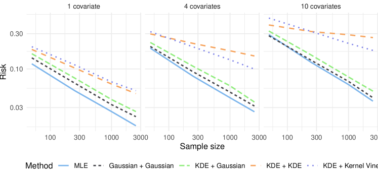
Figure 1: Average risk for expectile and quantile regression in a linear Gaussian model. Both axes have logarithmic scale.

There are two main observations. First, all parametric and semiparametric methods appear to converge at $\sqrt{n}$ rate, as seen from the $-1/2$ slopes. As expected from Corollaries 1 and 2, the MLE is slightly more efficient than the parametric copula-based method, which itself is slighlty more efficient than the semiparametric copula-based method. Second, the convergence rate of the KDE + KDE estimator deteriorates with the number of covariates, in line with Corollary 3. The KDE + Kernel Vine estimator achieves a better rate of convergence, largely unaffected by the dimension, as suggested by our discussion following Corollary 3. This illustrates the potential advantage of structural copula models for nonparametric regression.

5.2 Bootstrap confidence intervals

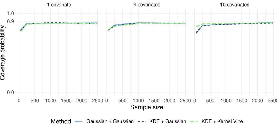
Figure 2: Coverage frequencies of bootstrapped 90%-confidence intervals.

We now consider the same setup, but compute 90% confidence intervals using 500 bootstrapped replicates. Because nonparametric estimators are generally biased, we have to undersmooth them to make the bias asymptotically negligible. In preliminary experiments, we discovered a small bias between the estimated regression target and its bootstrap replicates nevertheless. More details and a justification are given in the supplementary material.

The method KDE + KDE is omitted in these experiments because it is both heavily biased and computationally too demanding. In fig. 2, we observe that the coverage probabilities are all close to the target level of 90%. Coverage generally improved for larger sample sizes, but is insufficient for very small samples with $n=50$. Additional results for all sample sizes and the uncorrected bootstrap are in the supplementary materials.

5.3 Comparison to other methods

We conclude with a comparison of the KDE + Kernel Vine estimator from the previous section, Copula in the following, to three quantile regression benchmarks: linear quantile regression (LQR, Koenker 2022), support vector machines (SVM, Karatzoglou et al. 2004), and gradient boosted trees (GBM, Greenwell et al. 2020). All implementations are used with default parameters.

We simulate from two models with $d=10$ covariates. The first is the Gaussian from the previous section with marginal distributions of the response and covariates transformed respectively to lognormal and exponential. The second is a cubic additive model with three active covariates, namely $Y=(X_{1}+X_{2}+X_{3})^{3}+\epsilon$, where $X_{1},\dots,X_{10}$ and $\epsilon$ as before.

Using a test sample of size 250, we compare the estimators in two ways. First, we estimate conditional quantiles at levels 0.5 and 0.95, and report the average absolute distance from the true conditional quantiles. Second, we estimate conditional quantiles at all levels in $\{0.05,0.1,\cdots,0.9,0.95\}$, and report the fraction of observations where a $\tau_{1}$-quantile and a $\tau_{2}$-quantile with a certain gap $\tau_{1}-\tau_{2}$ cross. All results are based on 100 replications.

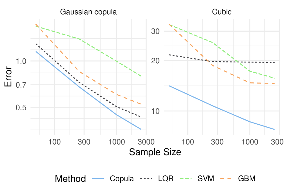
Figure 3: Average absolute test error of the conditional quantiles.

Table 1: Fraction of test points with quantile crossing.

gap	Copula	LQR	SVM	GBM
0.05	0%	52%	42%	99%
0.10	0%	37%	16%	75%
0.30	0%	27%	1%	22%

Figure 3 indicates that our method outperforms the benchmarks for both models. This was expected from the Gaussian, which amounts to a copula regression, but not necessarily from the cubic. Table 1 further shows that our method satisfy the monotonicity constraints of conditional quantiles, which is not the case for the benchmarks. GBM quantiles almost always cross when the gap is 0.05, on 22% of the samples even at a gap as large as 0.3. SVM and LQR do only slightly better. Depending on context, such behavior may be prohibitive. Quantiles predicted by our method never cross.

6.   Application: quantitative asset allocation

We revisit the application mentioned in Section 1 and illustrate how our method can help blend (subjective) economic views in an otherwise quantitative asset allocation. Suppose that an investor faces the problem of shifting the fraction of her total wealth across various categories to take advantage of evolving market conditions. Such categories might be asset classes, such as bonds, stocks, and commodities, or industry sectors in a stock portfolio. She might also need to evaluate a range of performance and risk measures for different portfolios under economic scenarios like “the GDP will grow by 0.5%” or “the unemployment rate will decrease by 1%”, over a given horizon.

Denote by ${\bm{Y}}\in{\mathbb{R}}^{d}$, ${\bm{\gamma}}\in{\mathbb{R}}^{d}$, and ${\bm{X}}\in{\mathbb{R}}^{p}$ the returns on the different categories, the fractions of total wealth invested in each of them, and the covariates. As measures of portfolio performance and risk, we consider the conditional mean, standard deviation or volatility, and 95% Value-at-Risk (VaR, see e.g., McNeil et al. 2015), defined respectively as $\mu_{{\bm{\gamma}}}^{*}={\mathrm{E}}({\bm{\gamma}}^{\top}{\bm{Y}}\mid{\bm{X}}={\bm{x}})$, $\sigma_{{\bm{\gamma}}}^{*}=\mathrm{var}({\bm{\gamma}}^{\top}{\bm{Y}}\mid{\bm{X}}={\bm{x}})^{1/2}$, and $q_{{\bm{\gamma}}}^{*}=F_{-{\bm{\gamma}}^{\top}{\bm{Y}}\mid{\bm{X}}}^{-1}(0.95\mid{\bm{x}})$.

Let the indexing set be $T=\{1,2,3\}\times\Gamma$, where $\Gamma=\{{\bm{\gamma}}\colon\sum_{j}\gamma_{j}=1,\max_{j}|\gamma_{j}|\leq M\}$ for some $M$ representing a constraint on how large a position in a single category can get. The parameter space and identifying functions are $\Theta=\{\theta_{t}\colon t\in T\}=\{\theta_{(j,{\bm{\gamma}})}\colon j\in\{1,2,3\},{\bm{\gamma}}\in\Gamma\}$ and ${\mathcal{G}}=\{g_{\theta,t}\colon t\in T\}=\{g_{\theta,(j,{\bm{\gamma}})}\colon j\in\{1,2,3\},{\bm{\gamma}}\in\Gamma\}$, where

$$\theta_{t}=\theta_{(j,{\bm{\gamma}})}=\begin{cases}\mu_{{\bm{\gamma}}},\quad&j=1\\ \sigma_{{\bm{\gamma}}},\quad&j=2\\ q_{{\bm{\gamma}}},\quad&j=3\end{cases}\qquad g_{\theta,t}=g_{\theta,(j,{\bm{\gamma}})}=\begin{cases}{\bm{\gamma}}^{\top}{\bm{y}}-\mu_{{\bm{\gamma}}},\quad&j=1\\ ({\bm{\gamma}}^{\top}{\bm{y}}-\mu_{{\bm{\gamma}}})({\bm{\gamma}}^{\top}{\bm{y}}-\mu_{{\bm{\gamma}}})^{\top}-\sigma_{{\bm{\gamma}}}^{2},\quad&j=2\\ 0.95-\mathds{1}(-{\bm{\gamma}}^{\top}{\bm{y}}<q_{{\bm{\gamma}}}),\quad&j=3\end{cases}.$$

With $\{\bm{e}_{i}\}_{i=1}^{d}$ the standard basis of ${\mathbb{R}}^{d}$, $t=(1,\bm{e}_{i})$ and $t=(2,\bm{e}_{i})$ correspond respectively to the conditional expected return and variance of asset $i$, and $t=(2,\bm{e}_{i}+\bm{e}_{j})$ to the conditional covariance between assets $i$ and $j$. This formulation thus also identifies the vector of expected returns ${\bm{\mu}}^{*}={\mathrm{E}}({\bm{Y}}\mid{\bm{X}}={\bm{x}})$ and the covariance matrix ${\bm{\Sigma}}^{*}=\mathrm{cov}({\bm{Y}}\mid{\bm{X}}={\bm{x}})$.

Given an estimated weight $\widehat{w}$, $\widehat{q}_{{\bm{\gamma}}}$ has to be solved for numerically, but there are closed form solutions for the conditional mean vector and covariance matrix estimators, that is

$$\widehat{\bm{\mu}}=\frac{\sum_{i=1}^{n}\bm{Y}_{i}\widehat{w}({\bm{Y}}_{i})}{\sum_{i=1}^{n}\widehat{w}({\bm{Y}}_{i})},\qquad\widehat{\bm{\Sigma}}=\frac{\sum_{i=1}^{n}(\bm{Y}_{i}-\widehat{\bm{\mu}})(\bm{Y}_{i}-\widehat{\bm{\mu}})^{\top}\widehat{w}({\bm{Y}}_{i})}{\sum_{i=1}^{n}\widehat{w}({\bm{Y}}_{i})},$$

leading to $\widehat{\mu}_{{\bm{\gamma}}}={\bm{\gamma}}^{\top}\widehat{\bm{\mu}}$ and $\widehat{\sigma}_{{\bm{\gamma}}}=\sqrt{{\bm{\gamma}}^{\top}\widehat{\bm{\Sigma}}{\bm{\gamma}}}$.

If for all ${\bm{\gamma}}\in\Gamma$, ${\bm{\theta}}_{{\bm{\gamma}}}=(\mu_{{\bm{\gamma}}},\sigma_{{\bm{\gamma}}},q_{{\bm{\gamma}}})$ lies in a compact subset of ${\mathbb{R}}\times{\mathbb{R}}_{>0}\times{\mathbb{R}}_{>0}$, the collection of identifying functions ${\mathcal{G}}$ satisfies the conditions of our theorems. Thus, our results in Section 4 imply that the estimators $\widehat{\bm{\theta}}_{{\bm{\gamma}}}=(\widehat{\mu}_{{\bm{\gamma}}},\widehat{\sigma}_{{\bm{\gamma}}},\widehat{q}_{{\bm{\gamma}}})$ are consistent, converge weakly, and that their bootstrap versions yield valid inferences, uniformly in ${\bm{\gamma}}\in\Gamma$. To obtain uniform confidence bands over portfolios for the volatility and VaR, we compute the statistics $\widehat{\sigma}_{b}=\sup_{{\bm{\gamma}}\in\Gamma}\bigl{|}\widehat{\sigma}_{b,{\bm{\gamma}}}-\widehat{\sigma}_{{\bm{\gamma}}}\bigr{|}$ and $\widehat{q}_{b}=\sup_{{\bm{\gamma}}\in\Gamma}\bigl{|}\widehat{q}_{b,{\bm{\gamma}}}-\widehat{q}_{{\bm{\gamma}}}\bigr{|}$ for bootstrap samples $b=1,\dots,B$. Uniform $\alpha$-confidence bands are then given by ${\bm{\gamma}}\mapsto\widehat{\sigma}_{{\bm{\gamma}}}\pm\widehat{s}_{\sigma,\alpha}$ and ${\bm{\gamma}}\mapsto\widehat{q}_{{\bm{\gamma}}}\pm\widehat{s}_{q,\alpha}$, with $\widehat{s}_{\sigma,\alpha}$ and $\widehat{s}_{q,\alpha}$ respectively the $\alpha$-quantiles of $\widehat{\sigma}_{b}$ and $\widehat{q}_{b}$. Scripts to reproduce the following analysis with the eecop (Nagler & Vatter 2020a) package are in the supplementary material.

6.1 The data

For ${\bm{Y}}$, we use value-weighted returns on 5 industry portfolios. For ${\bm{X}}$, we use the real gross domestic product and the seasonally adjusted unemployment rate. With yearly data covering 1947-2019, we have a total of 72 observations. The average yearly returns on stocks are in the 13-17% range, but with large variations over time. While the GDP has been growing steadily at around 3% per year, the evolution of the unemployment has varied widely. Further, the returns on all industry sectors are positively correlated among each other and the growth in GDP, and negatively correlated with the growth in unemployment. Because the auto-correlations of all variables and their squares are statistically indistinguishable from zero, we treat the data as iid. Plots of time-series, auto-correlation functions, cross-correlations and summary statistics, along with additional details on the data sources, are in the supplementary material.

To study the impact of the predictors in the quantitative allocation scheme, we create three scenarios for the change in GDP and unemployment: good economy (+4.35/-11.52), median economy (+3.22/-2.48), poor economy (+1.59/+5.44). The good and bad scenarios are obtained using the 75th and 25th percentile for the growth in GDP unemployment, and conversely for the unemployment.

6.2 Results

To derive predictions for each scenario, we estimate all margins by kernel estimators with plug-in bandwidths and fit a parametric vine copula model for the copula density. Predicted conditional means, standard deviations, and 95% VaRs are given in Table 2. We see that, the better the economic outlook, the higher the expected returns, and the lower the risk.

Table 2: Predicted means ($\mu$), standard deviations ($\sigma$), and VaRs ($q$) for each scenario.

	Cnsmr			Manuf			HiTec			Hlth			Other
Scenario	$\mu$	$\sigma$	$q$	$\mu$	$\sigma$	$q$	$\mu$	$\sigma$	$q$	$\mu$	$\sigma$	$q$	$\mu$	$\sigma$	$q$
Good economy	17.7	15.0	3.7	17.5	13.1	7.2	17.5	18.2	11.8	17.9	18.6	12.1	18.4	16.5	9.2
Median economy	16.1	15.9	5.4	14.7	13.4	11.1	15.6	18.9	16.6	16.2	18.3	12.2	15.2	16.7	9.8
Poor economy	9.1	16.6	13.2	8.0	14.2	12.8	9.5	20.1	25.0	11.1	17.6	17.3	7.1	17.0	18.8

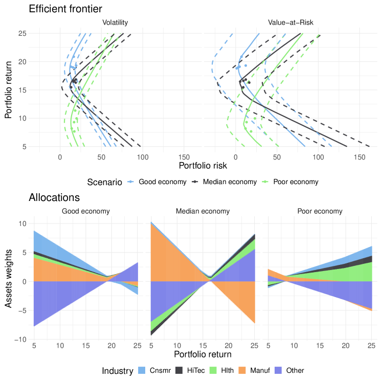
Figure 4: Efficient frontiers with uniform 75%-confidence bands and scatterplots for the individual assets (top panel), and corresponding portfolio weights (bottom panel).

For each scenario, we compute the efficient frontier, that is a set of portfolios where ${\bm{\gamma}}$ can be expressed as a linear combination of the minimum variance and market portfolios. Background details on asset allocation can be found in the supplementary material. In the top panel of Figure 4, we show the frontiers as a lineplot with uniform 75% bands as the dashed lines, and the corresponding quantities for the individual assets as a scatterplot. In the bottom panel, the portfolio weights are displayed as a function of the expected return. We can make the following observations:

• The upper half of all the parabolas yields higher returns for the same risk compared with the lower half, rational investors would only choose such portfolios.

• Similarly, since the scatterpoints corresponding to the individual assets are “inside” the parabolas, rational investors would prefer diversified portfolios from the upper half.

• Better economic outlooks generally imply higher expected returns at a given risk level.

• The weights of efficient portfolios with returns between that of minimum variance and market portfolios are generally reasonable, that is mostly included in $[-1,1]$. And targeting returns outside this range generally requires large long and short positions, accompanied by quick an increase in portfolio risk.

Nonetheless, the uncertainties are fairly large, due to the small sample size. In higher frequency data (e.g., monthly) however, serial dependence can no longer be ignored. An extension of our results to this setting is discussed briefly in the following section.

7.   Discussion

Section 4 provides an umbrella theory for solutions to copula-based estimating equations, and has close connections to several recent results. Noh et al. (2013) shows consistency and asymptotic normality for mean regression in a semiparametric model. Noh et al. (2015) and De Backer et al. (2017) derive similar results for quantile regression, the latter for semiparametric copula densities. Rémillard et al. (2017) establish weak convergence of parametetric and semiparametric estimators and validity of a parametric bootstrap procedure for the conditional quantile function indexed by the level. Note that Noh et al. (2015) replace the iid-assumption by a mixing condition, which we do not cover. But our results can likely be extended to stationary sequences under more stringent conditions using the techniques in Dehling et al. (2002). Nonetheless, we generalize and extend the above in several ways:

• The focus of previous research is on mean and quantile regression with univariate response. We allow for large classes of potentially multivariate identifying functions. This opens new possibilities for copula-based solutions to other regression problems.

• Previous results cover only parametric or semiparametric copula estimators. Our theory allows for parametric, semiparametric, and nonparametric methods.

• Weak convergence of $\widehat{\theta}$ as a process indexed by some potentially dense set $T$ is established. It can be used to derive simultaneous and coherent inferences across arbitrary combinations of finite/infinite-dimensional features of the conditional distribution.

• We propose and validate a bootstrapping scheme. It is applicable whenever obtaining the asymptotic distribution in closed form is inconvenient or infeasible.

• The theory also applies to M-estimators, defined as maximizers of a criterion function, when the criterion is differentiable (see, e.g., Kosorok 2007, Section 2.2.6).

• Our results apply to both continuous and discrete data. Admittedly, the practical applicability for discrete data is limited by a lack of available software. While experimental features for discrete variables exist in the rvinecopulib package (Nagler & Vatter 2020b), they still need to mature. But the theoretical foundation is set and we hope that the computational limitations are overcome in the near future.

Being broadly applicable, our main results are somewhat abstract. But it is often straightforward to specialize them given a specific identifying function and weight estimator, as we do in Corollaries 1 to 3. We close our discussion by outlining applications to additional regression problems covered by our theory in Section 4.

First, suppose the goal is to characterize the relationship between a response $Y_{1}$ and a treatment $Y_{2}$ using an instrument $Y_{3}$, conditionally on a set of exogenous covariates ${\bm{X}}$. Specifically, assume as in Newey & Powell (2003) that $Y_{1}=\bm{b}(Y_{2})^{\top}\bm{{\bm{\theta}}}({\bm{X}})+Z$, where $\bm{b}$ is known vector of basis functions, and $Z$ is a zero-mean error term. When the treatment is endogenous, that is $Y_{2}\not\mathchoice{\mathrel{\hbox to0.0pt{$\displaystyle\perp$\hss}\mkern 2.0mu{\displaystyle\perp}}}{\mathrel{\hbox to0.0pt{$\textstyle\perp$\hss}\mkern 2.0mu{\textstyle\perp}}}{\mathrel{\hbox to0.0pt{$\scriptstyle\perp$\hss}\mkern 2.0mu{\scriptstyle\perp}}}{\mathrel{\hbox to0.0pt{$\scriptscriptstyle\perp$\hss}\mkern 2.0mu{\scriptscriptstyle\perp}}}Z$, identifying ${\bm{\theta}}$ requires an instrument $Y_{3}$ satisfying $E(Z\mid{\bm{X}}={\bm{x}},Y_{3}=y_{3})=0$ for all ${\bm{x}}$ and $y_{3}$. In other words, one has to solve ${\mathrm{E}}\bigl{(}Y_{1}|{\bm{X}}={\bm{x}},Y_{3}=y_{3}\bigr{)}=E\bigl{\{}\bm{b}(Y_{2})^{\top}\bm{{\bm{\theta}}}({\bm{X}})|{\bm{X}}={\bm{x}},Y_{3}=y_{3}\bigr{\}}$ for all ${\bm{x}}$ and $y_{3}$. Then the collection ${\mathcal{G}}=\{g_{{\bm{\theta}},t}\colon{\bm{\theta}}\in\Theta,t\in T\}$ with $g_{{\bm{\theta}},t}({\bm{y}})=b_{t}(y_{3})\bigl{\{}y_{1}-\bm{b}(y_{2})^{\top}{\bm{\theta}}\bigr{\}}$ identifies the parameter $\bm{\theta}(\bm{x})$ for given $\bm{x}$. In the supplement, we show that 2 and 8 are satisfied, and it is then left to check 3 to 7 and 9.

Further, our results apply to problems with censored or missing responses by tweaking the weight function. For example, suppose we only observe the right-censored version $\bar{S}=\min(S,Z)\in{\mathbb{R}}$ of a survival time $S$, along with a censoring indicator $\Delta=\mathds{1}(S\leq Z)$. For any identifying function $\phi_{\theta}$, ${\mathrm{E}}\bigl{\{}\phi_{\theta}(S)\mid{\bm{X}}={\bm{x}}\bigr{\}}=0$ if and only if $E\bigl{\{}\phi_{\theta}(\bar{S})\Delta\bar{w}^{*}(\bar{S})\zeta(\bar{S})\bigr{\}}=0$, where $\zeta(t)=1/\{1-F_{Z\mid{\bm{X}}}(t\mid{\bm{x}})\}$ and $\bar{w}^{*}$ is defined as in (2), but replacing $F_{Y,{\bm{X}}}$ and $F_{Y}$ by $F_{\bar{S},{\bm{X}}}$ and $F_{\bar{S}}$. This technique was used in De Backer et al. (2017) to allow for right censoring in copula-based quantile regression, and it fits the setup of Section 4. With ${\bm{Y}}=(\bar{S},\Delta)$, $g_{\theta}({\bm{y}})=\phi_{\theta}(y_{1})y_{2}$, and ${w^{*}}({\bm{y}})=\bar{w}^{*}(y_{1})\zeta(y_{1})$, then $E\bigl{\{}\phi_{\theta}(\bar{S})\Delta\bar{w}^{*}(\bar{S})\zeta(\bar{S})\bigr{\}}=E\bigl{\{}g_{\theta}({\bm{Y}}){w^{*}}({\bm{Y}})\bigr{\}}$ and it remains to check the assumptions of Theorems 1 to 3. The above is only one instance of a larger class of methods based on inverse probability weighting. Other weight functionals $\zeta$ can be used similarly to account for other forms of censoring and missingness (see, e.g. Robins et al. 1994, Wooldridge 2007, Han et al. 2016). Following an earlier version of this paper that appeared online, this idea was already picked by Hamori et al. (2020), albeit in a restricted semiparametric context.

Acknowledgements

The authors thank Johannes Wiesel for the proof of Lemma 11 in the supplementary material. We are grateful to the Associate Editor and three referees for helpful comments. Part of the research was conducted while Thomas Nagler was at Delft University of Technology and Thibault Vatter was at Columbia University.

Funding

Thomas Nagler was partially supported by a Spinoza grant awarded by the Netherlands Organisation of Scientific Research (NWO). Thibault Vatter was partially supported by the Swiss National Science Foundation (Grant 174709).

Appendix A Assumptions

In general, we assume that the parameter space satisfies $\Theta\subseteq\ell^{\infty}(T)$ for some indexing set $T$. For simplicity, we consider $T$ to be a compact subset of a Euclidean space. We also use $({\bm{Y}}^{\prime},{\bm{X}}^{\prime})$ to denote an independent copy of $({\bm{Y}},{\bm{X}})$.

A.1 Assumptions for the main results

Assumption 1.

The parameter space $\Theta$ is compact and contains an interior point ${\theta^{*}}\in\Theta$ such that $E\{g_{{\theta^{*}}}({\bm{Y}}){w^{*}}({\bm{Y}})\}=0$ and, for any $\epsilon>0$, $\inf_{|\theta_{t}-{\theta_{t}^{*}}|>\epsilon,t\in T}|E\{g_{\theta,t}({\bm{Y}}){w^{*}}({\bm{Y}})\}|>0$.

Assumption 2.

The class ${\mathcal{G}}=\{g_{\theta}\colon\theta\in\Theta\}$ is Euclidean for some envelope function $G$.

Assumption 3.

There exists a sequence of functions $w_{n}\colon{\mathbb{R}}^{2d+p}\to{\mathbb{R}}$ and a sequence $r_{n}=o(n^{1/2})$ with $r_{n}\geq 1$, such that $\max_{1\leq i\leq n}\biggl{|}\widehat{w}({\bm{Y}}_{i})-\frac{1}{n}\sum_{j=1}^{n}w_{n}({\bm{Y}}_{i},{\bm{Y}}_{j},{\bm{X}}_{j})\biggr{|}=o_{P}\bigl{(}n^{-1/2}r_{n}\bigr{)}$.

Assumption 4.

$\sup_{\theta\in\Theta}\|{\mathrm{E}}\{g_{\theta}({\bm{Y}})w_{n}({\bm{Y}},{\bm{Y}}^{\prime},{\bm{X}}^{\prime})\}-{\mathrm{E}}\{g_{\theta}({\bm{Y}}){w^{*}}({\bm{Y}})\}\|_{T}=o(1)$.

Assumption 5.

$G$, $w_{n}$, and $r_{n}$ are such that

1. ${\mathrm{E}}\{|G({\bm{Y}})|\}<\infty$,

2. ${\mathrm{E}}\{G({\bm{Y}})|w_{n}({\bm{Y}},{\bm{Y}},{\bm{X}})|\}=o(n^{1/2}r_{n})$,

3. ${\mathrm{E}}\{G({\bm{Y}})^{2}w_{n}({\bm{Y}},{\bm{Y}}^{\prime},{\bm{X}}^{\prime})^{2}\}=o(nr_{n}^{2})$.

Assumption 6.

With $({\bm{y}}^{\prime},{\bm{x}}^{\prime})$ an arbitrary point in ${\mathcal{Y}}\times{\mathcal{X}}$, the functions

$$h_{n,\theta,t}({\bm{y}}^{\prime},{\bm{x}}^{\prime}) ={\mathrm{E}}\{g_{\theta,t}({\bm{Y}})w_{n}({\bm{Y}},{\bm{y}}^{\prime},{\bm{x}}^{\prime})+g_{\theta,t}({\bm{y}}^{\prime})w_{n}({\bm{y}}^{\prime},{\bm{Y}},{\bm{X}})\},$$

$$H_{n}({\bm{y}}^{\prime},{\bm{x}}^{\prime}) ={\mathrm{E}}\{G({\bm{Y}})|w_{n}({\bm{Y}},{\bm{y}}^{\prime},{\bm{x}}^{\prime})|+G({\bm{y}}^{\prime})|w_{n}({\bm{y}}^{\prime},{\bm{Y}},{\bm{X}})|\},$$

satisfy

1. $\sup_{\|\theta_{1}-\theta_{2}\|_{T}+\|t_{1}-t_{2}\|<\delta_{n}}{\mathrm{E}}\{|h_{n,\theta_{1},t_{1}}({\bm{Y}}^{\prime},{\bm{X}}^{\prime})-h_{n,\theta_{2},t_{2}}({\bm{Y}}^{\prime},{\bm{X}}^{\prime})|^{2}\}=o(r_{n}^{2})$ for every $\delta_{n}\to 0$,

2. ${\mathrm{E}}\{r_{n}^{-2}H_{n}({\bm{Y}}^{\prime},{\bm{X}}^{\prime})^{2}\}=O(1)$,

3. ${\mathrm{E}}\{r_{n}^{-2}H_{n}({\bm{Y}}^{\prime},{\bm{X}}^{\prime})^{2}\mathds{1}_{r_{n}^{-1}H_{n}({\bm{Y}}^{\prime},{\bm{X}}^{\prime})\geq\eta\sqrt{n}}\}=o(1)$ for every $\eta>0$.

Assumption 7.

$\|{\mathrm{E}}[\{g_{\theta_{n}}({\bm{Y}})-g_{{\theta^{*}}}({\bm{Y}})\}\{w_{n}({\bm{Y}},{\bm{Y}}^{\prime},{\bm{X}}^{\prime})-{w^{*}}({\bm{Y}})\}]\|_{T}=o(\|\theta_{n}-{\theta^{*}}\|_{T})$ for every $\theta_{n}\to{\theta^{*}}$.

Assumption 8.

The map $\theta\mapsto{\mathrm{E}}\{g_{\theta}({\bm{Y}}){w^{*}}({\bm{Y}})\}$ from $\ell^{\infty}(T)$ to $\ell^{\infty}(T)$ is Fréchet differentiable in a neighborhood of ${\theta^{*}}$ and the derivative $V_{\theta}\colon\ell^{\infty}(T)\mapsto\ell^{\infty}(T)$ is invertible at ${\theta^{*}}$. That is, for $\theta$ in a neighborhood of ${\theta^{*}}$, $V_{\theta}$ is a bounded linear operator such that

$$\|{\mathrm{E}}\{g_{\theta_{n}}({\bm{Y}}){w^{*}}({\bm{Y}})\}-{\mathrm{E}}\{g_{\theta}({\bm{Y}}){w^{*}}({\bm{Y}})\}-V_{\theta}(\theta_{n}-\theta)\|_{T}=o(\|\theta_{n}-\theta\|_{T}),\quad\forall\theta_{n}\to\theta.$$

And the inverse is the map $V_{{\theta^{*}}}^{-1}$ such that $V_{{\theta^{*}}}^{-1}V_{{\theta^{*}}}$ is the identity.

Assumption 9.

There are iid random variables $\xi_{i},i=1,\dots,n$ independent of $({\bm{Y}}_{i},{\bm{X}}_{i})_{i=1}^{n}$ with ${\mathrm{E}}(\xi_{1})=\mathrm{var}(\xi_{1})=1$, and ${\mathrm{E}}\{|\xi_{1}|^{2+\epsilon}\}<\infty$ for some $\epsilon<0$, such that for the same $w_{n},r_{n}$ as in 3, $\max_{1\leq i\leq n}\biggl{|}\widetilde{w}({\bm{Y}}_{i})-\frac{1}{n}\sum_{j=1}^{n}\xi_{i}w_{n}({\bm{Y}}_{i},{\bm{Y}}_{j},{\bm{X}}_{j})\biggr{|}=o_{P}\bigl{(}n^{-1/2}r_{n}\bigr{)}$.

A brief discussion of the assumptions is in order. 1 ensures identifiability of the parameter of interest ${\theta^{*}}$. 2 limits the complexity of the class of identifying functions ${\mathcal{G}}=\{g_{\theta}\colon\theta\in\Theta\}$. Importantly, this complexity is disentangled from the weight estimator. Euclidean classes (Nolan & Pollard 1987) generalize Vapnik-Cervonenkis classes of real-valued functions and are also called VC-type classes by some authors (e.g., Giné & Koltchinskii 2006). A formal definition and several convenient properties of these classes are in the supplementary material, where we also verify 2 for all examples from Section 3.1. 3 allows us to expand $\widehat{w}$ as a sample average and a uniformly negligible remainder. Since we only evaluate $\widehat{w}$ on ${\bm{Y}}_{1},\dots,{\bm{Y}}_{n}$ in the empirical estimating equation (7), the expansion only needs to be valid at these points. 9 is an analogous condition for $\widetilde{w}$, the bootstrap version of $\widehat{w}$. 4 ensures consistency of $\widehat{w}$ to ${w^{*}}$ in a weak sense. In particular, we require neither uniform nor pointwise consistency, although, with 5, either can be shown to be sufficient.

The remaining assumptions deal with joint regularity of the class of identifying functions ${\mathcal{G}}$ and the weight estimator $\widehat{w}$ through the sequence $w_{n}$. 5 and Items 6ii to 6iii are moment conditions. In the latter two, the randomness from either estimating ${w^{*}}$ or replacing the population mean by its empirical counterpart has been averaged out; see also the discussion following Theorem 2. Item 6i is a form of stochastic equicontinuity in both $\theta$ and $t$. Note that Items 6i to 6iii are common in the context of function classes changing with $n$ (see e.g., van der Vaart & Wellner 1996, Section 2.11.3). 8 ensures sufficient smoothness of the map $\theta\mapsto{\mathrm{E}}\{g_{\theta}({\bm{Y}}){w^{*}}({\bm{Y}})\}$ and is verified in the supplementary material for the examples from Section 3.1. It could be weakened to Hadamard differentiability at the cost of slightly more tedious proofs. 7 ensures that replacing ${w^{*}}$ by $\widehat{w}$ has a negligible effect on the smoothness in 8.

When specifying $\widehat{w}$ further, the assumptions can often be disentangled into separate conditions on the identifying functions and weight estimator, see 10 to 12 below.

A.2 Assumptions for the corollaries

Assumption 10.

Denote respectively by ${w^{*}}({\bm{y}})=w({\bm{y}};\bm{\eta}^{*})$ and $\widehat{w}({\bm{y}})=w({\bm{y}};\bm{\widehat{\eta}})$ the true and estimated weight functions.

1. One has $\bm{\widehat{\eta}}-\bm{\eta}^{*}=\frac{1}{n}\sum_{i=1}^{n}\bm{\gamma}({\bm{Y}}_{i},{\bm{X}}_{i})+o_{P}(n^{-1/2})$ and $\bm{\widetilde{\eta}}-\bm{\eta}^{*}=\frac{1}{n}\sum_{i=1}^{n}\xi_{i}\bm{\gamma}({\bm{Y}}_{i},{\bm{X}}_{i})+o_{P}(n^{-1/2})$, for a function $\bm{\gamma}$ with ${\mathrm{E}}\{\bm{\gamma}({\bm{Y}},{\bm{X}})\}=0$ and ${\mathrm{E}}\{\|\bm{\gamma}({\bm{Y}},{\bm{X}})\|_{2}^{2+\epsilon}\}<\infty$ and iid positive random variables $\xi_{1},\dots,\xi_{n}$ independent of $({\bm{Y}}_{i},{\bm{X}}_{i})_{i=1}^{n}$ with ${\mathrm{E}}(\xi_{1})=\mathrm{var}(\xi_{1})=1$ and ${\mathrm{E}}\{|\xi_{1}|^{2+\epsilon}\}<\infty$ for some $\epsilon<0$.

2. The function $w({\bm{y}};\bm{\eta}^{*})$ is twice continuously differentiable in $\bm{\eta}^{*}$ with derivatives uniformly bounded in ${\bm{y}}\in{\mathcal{Y}}$.

3. One has ${\mathrm{E}}\{w({\bm{Y}};\bm{\eta}^{*})^{2}+\|\nabla_{\bm{\eta}}w({\bm{Y}};\bm{\eta}^{*})\|_{2}^{2}\}<\infty$.

4. For some $\epsilon>0$, one has ${\mathrm{E}}\{G({\bm{Y}})^{2+\epsilon}\mid{\bm{X}}={\bm{x}}\}<\infty$ and ${\mathrm{E}}\{G({\bm{Y}})^{2+\epsilon}\}$.

5. For every $\delta_{n}\to 0$ and with $\|\cdot\|$ the Euclidean norm, one has

   $$\sup_{\|\theta_{1}-\theta_{2}\|_{T}+\|t_{1}-t_{2}\|<\delta_{n}}{\mathrm{E}}\bigl{\{}|g_{\theta_{1},t_{1}}({\bm{Y}})-g_{\theta_{2},t_{2}}({\bm{Y}})|^{2}\mid{\bm{X}}={\bm{x}}\bigr{\}}=o(1),$$

   $$\sup_{\|\theta_{1}-\theta_{2}\|_{T}+\|t_{1}-t_{2}\|<\delta_{n}}\bigl{\|}{\mathrm{E}}\bigl{\{}|g_{\theta_{1},t_{1}}({\bm{Y}})-g_{\theta_{2},t_{2}}({\bm{Y}})|^{2}\bigr{\}}\bigr{\|}_{2}=o(1).$$

Assumption 11.

Write ${\bm{F}}_{{\bm{Y}}}({\bm{y}})=(F_{Y_{1}}(y_{1}),\dots,F_{Y_{d}}(y_{d}))$ and similarly for ${\bm{F}}_{{\bm{X}}}$, $\widehat{\bm{F}}_{{\bm{Y}}}$, and $\widehat{\bm{F}}_{{\bm{X}}}$. Define $\omega({\bm{u}},{\bm{v}};\bm{\eta})=c_{{\bm{Y}},{\bm{X}}}({\bm{u}},{\bm{v}};\bm{\eta})/c_{{\bm{Y}}}({\bm{u}};\bm{\eta})$, $w({\bm{y}};\bm{\eta})=\omega\{{\bm{F}}_{\bm{Y}}({\bm{y}}),{\bm{F}}_{\bm{X}}({\bm{x}});\bm{\eta}\}$, and

$$\lambda({\bm{Y}},{\bm{X}}) =\sum_{j=1}^{d}\int g_{{\theta^{*}}}({\bm{y}})\frac{\partial\omega\{\bm{F}_{\bm{Y}}({\bm{y}}),\bm{F}_{\bm{X}}({\bm{x}});\bm{\eta}^{*}\}}{\partial F_{Y_{j}}(y_{j})}\times\{\mathds{1}(Y_{j}\leq y_{j})-F_{Y_{j}}(y_{j})\}f_{\bm{Y}}({\bm{y}})d{\bm{y}}$$

$$\quad+\sum_{k=1}^{p}\frac{\partial{\mathrm{E}}\bigl{\{}g_{{\theta^{*}}}({\bm{Y}})\mid{\bm{X}}={\bm{x}}\bigr{\}}}{\partial x_{k}}\times\frac{\{\mathds{1}(X_{k}\leq x_{k})-F_{X_{k}}(x_{k})\}}{f_{X_{k}}(x_{k})}.$$

Further, for any $Z\in\{Y_{1},\dots,Y_{d},X_{1},\dots,X_{p}\}$, write $\widetilde{F}_{Z}(z)=n^{-1}\sum_{i=1}^{n}\xi_{i}\mathds{1}(Z_{i}\leq z)$ for the bootstrapped empirical distribution.

1. Items 10i, 10iv and 10v hold.

2. The function $(\bm{u},\bm{v},\bm{\eta})\mapsto\omega(\bm{u},\bm{v};\bm{\eta})$ has two continuous derivatives on the domain $[0,1]^{d}\times\{\bm{v}\colon\|\bm{v}-{\bm{F}}_{\bm{X}}({\bm{x}})\|<\epsilon\}\times\{\bm{\eta}\colon\|\bm{\eta}-\bm{\eta}^{*}\|<\epsilon\}$ for some $\epsilon>0$.

3. One has ${\mathrm{E}}\{\omega({\bm{Y}},{\bm{X}};\bm{\eta}^{*})^{2}+\|\nabla_{(\bm{\eta},{\bm{Y}},{\bm{X}})}\omega({\bm{Y}},{\bm{X}};\bm{\eta}^{*})\|_{2}^{2}\}<\infty$.

Assumption 12.

l

1. $K$ is a symmetric, bounded probability density function on $[-1,1]$.

2. One has $b_{n},\sigma_{n}\to 0$, $b_{n}^{2}=o(n^{-1/2}\sigma_{n}^{-p/2})$, $\sigma_{n}^{-p/2}b_{n}^{d}/\ln n\to\infty$, and $nb_{n}^{d}\sigma_{n}^{p}/\ln n\to\infty$.

3. The densities $f_{\bm{X},{\bm{Y}}}$ and $f_{\bm{Y}}$ have uniformly bounded and continuous derivatives up to the third order and $\sup_{{\bm{y}}\in{\mathcal{Y}}}f_{\bm{X}\mid{\bm{Y}}}({\bm{x}}\mid{\bm{y}})<\infty$.

4. One has $\lim_{\delta\to 0}\sup_{{\bm{y}}\in{\mathcal{Y}}}\sup_{\|{\bm{y}}^{\prime}-{\bm{y}}\|\leq\delta}\sup_{\|{\bm{x}}^{\prime}-{\bm{x}}\|\leq\delta}\biggl{|}\frac{f_{{\bm{Y}},\bm{X}}({\bm{y}}^{\prime},{\bm{x}}^{\prime})}{f_{{\bm{Y}},\bm{X}}({\bm{y}},{\bm{x}})}-1\biggr{|}=0$.

5. For some $\epsilon,\delta>0$, one has ${\mathrm{E}}\{\sup_{|\bm{a}|<\delta}G({\bm{Y}}+\bm{a})^{2+\epsilon}\mid{\bm{X}}={\bm{x}}\}<\infty$ and ${\mathrm{E}}\{G({\bm{Y}})^{2+\epsilon}\}$.

6. For every $\theta_{n}\to{\theta^{*}}$ and $\delta_{n}\to 0$ and with $\|\cdot\|$ the Euclidean norm, one has

   $$\bigl{\|}{\mathrm{E}}\bigl{\{}|g_{\theta_{n}}({\bm{Y}})-g_{{\theta^{*}}}({\bm{Y}})|\mid{\bm{X}}={\bm{x}}\bigr{\}}\bigr{\|}_{T} =O(\|\theta_{n}-{\theta^{*}}\|_{T}),$$

   $$\sup_{\|\theta_{1}-\theta_{2}\|_{T}+\|t_{1}-t_{2}\|<\delta_{n}}{\mathrm{E}}\bigl{\{}|g_{\theta_{1},t_{1}}({\bm{Y}})-g_{\theta_{2},t_{2}}({\bm{Y}})|^{2}\mid{\bm{X}}={\bm{x}}\bigr{\}} =o(1).$$

In all three cases, the specialized assumptions 10 to 12 are standard regularity conditions on the estimation method, as well as smoothness and moment conditions for the identifying function. This is in contrast to the general conditions 3, 5, 4, 6, 7 and 9, where the estimation method and identifying function are often intertwined. Unfortunately, to the best of our knowledge, this disentanglement is not feasible in the general setting of Theorems 1 to 3 without strengthening the conditions.

See pages - of copula_ee_supplement.pdf

References

- (1)
- Bouyé & Salmon (2009) Bouyé, E. & Salmon, M. (2009), ‘Dynamic copula quantile regressions and tail area dynamic dependence in Forex markets’, The European Journal of Finance 15(7-8), 721–750.
- Bücher & Kojadinovic (2019) Bücher, A. & Kojadinovic, I. (2019), ‘A note on conditional versus joint unconditional weak convergence in bootstrap consistency results’, Journal of Theoretical Probability 32(3), 1145–1165.
- Cai & Zhang (2018) Cai, T. T. & Zhang, L. (2018), ‘High-dimensional gaussian copula regression: Adaptive estimation and statistical inference’, Statistica Sinica 28(2), 963–993.
- Carrera et al. (2019) Carrera, D., Bandeira, L., Santana, R. & Lozano, J. A. (2019), ‘Detection of sand dunes on mars using a regular vine-based classification approach’, Knowledge-Based Systems 163, 858–874.
- Chen et al. (2009) Chen, X., Koenker, R. & Xiao, Z. (2009), ‘Copula-based nonlinear quantile autoregression’, The Econometrics Journal 12(1), 50–67.
- Cooke et al. (2015) Cooke, R. M., Joe, H. & Chang, B. (2015), ‘Vine regression’, Resources for the Future - Discussion Paper 15(52), 15–52.
- Côté & Genest (2015) Côté, M.-P. & Genest, C. (2015), ‘A copula-based risk aggregation model’, The Canadian Journal of Statistics 43(1), 60–81.
- De Backer et al. (2017) De Backer, M., El Ghouch, A. & Van Keilegom, I. (2017), ‘Semiparametric copula quantile regression for complete or censored data’, Electronic Journal of Statistics 11(1), 1660–1698.
- Dehling et al. (2002) Dehling, H., Mikosch, T. & Sörensen, M. (2002), Empirical Process Techniques for Dependent Data, Springer Science & Business Media.
- Dette et al. (2014) Dette, H., Van Hecke, R. & Volgushev, S. (2014), ‘Some Comments on Copula-Based Regression’, Journal of the American Statistical Association 109(507), 1319–1324.
- Efron (1979) Efron, B. (1979), ‘Bootstrap methods: Another look at the jackknife’, The Annals of Statistics 7(1), 1–26.
- Elidan (2012) Elidan, G. (2012), Copula Network Classifiers (CNCs)., in ‘Artificial Intelligence and Statistics (AISTATS) Proceedings’, pp. 346–354.
- Fan & Gijbels (1996) Fan, J. & Gijbels, I. (1996), Local polynomial modelling and its applications, Chapman & Hall/CRC, Boca Raton, Fla.
- Genest et al. (1995) Genest, C., Ghoudi, K. & Rivest, L.-P. (1995), ‘A semiparametric estimation procedure of dependence parameters in multivariate families of distributions’, Biometrika 82(3), 543–552.
- Giné & Koltchinskii (2006) Giné, E. & Koltchinskii, V. (2006), ‘Concentration inequalities and asymptotic results for ratio type empirical processes’, The Annals of Probability 34(3), 1143–1216.
-
Greenwell et al. (2020)
Greenwell, B., Boehmke, B., Cunningham, J. & Developers, G.
(2020), gbm: Generalized Boosted
Regression Models.
R package version 2.1.8.
https://github.com/gbm-developers/gbm - Hamori et al. (2020) Hamori, S., Motegi, K. & Zhang, Z. (2020), ‘Copula-based regression models with data missing at random’, Journal of Multivariate Analysis 180, 104654.
- Han et al. (2013) Han, F., Zhao, T. & Liu, H. (2013), ‘Coda: High dimensional copula discriminant analysis’, Journal of Machine Learning Research 14(Feb), 629–671.
- Han et al. (2016) Han, P., Wang, L. & Song, P. X.-K. (2016), ‘Doubly robust and locally efficient estimation with missing outcomes’, Statistica Sinica 26(2), 691–719.
- Hofert et al. (2020) Hofert, M., Kojadinovic, I., Maechler, M. & Yan, J. (2020), ‘copula: Multivariate dependence with copulas’. R package version 0.999-20, URL: https://CRAN.R-project.org/package=copula.
- Karatzoglou et al. (2004) Karatzoglou, A., Smola, A., Hornik, K. & Zeileis, A. (2004), ‘kernlab – an S4 package for kernel methods in R’, Journal of Statistical Software 11(9), 1–20.
-
Koenker (2022)
Koenker, R. (2022), quantreg: Quantile
Regression.
R package version 5.94.
https://www.r-project.org - Kolev & Paiva (2009) Kolev, N. & Paiva, D. (2009), ‘Copula-based regression models: A survey’, Journal of Statistical Planning and Inference 139(11), 3847–3856.
- Kosorok (2007) Kosorok, M. R. (2007), Introduction to empirical processes and semiparametric inference, Springer Series in Statistics, Springer Science & Business Media.
- Kraus & Czado (2017) Kraus, D. & Czado, C. (2017), ‘D-vine copula based quantile regression’, Computational Statistics & Data Analysis 110, 1–18.
- McNeil et al. (2015) McNeil, A. J., Frey, R. & Embrechts, P. (2015), Quantitative Risk Management: Concepts, Techniques and Tools – revised edition, Princeton university press.
- Nagler & Czado (2016) Nagler, T. & Czado, C. (2016), ‘Evading the curse of dimensionality in nonparametric density estimation with simplified vine copulas’, Journal of Multivariate Analysis 151, 69–89.
- Nagler et al. (2017) Nagler, T., Schellhase, C. & Czado, C. (2017), ‘Nonparametric estimation of simplified vine copula models: comparison of methods’, Dependence Modeling 5(1), 99–120.
- Nagler & Vatter (2019) Nagler, T. & Vatter, T. (2019), ‘kde1d: Univariate kernel density estimation’. R package version 1.0.2, URL: https://CRAN.R-project.org/package=kde1d.
- Nagler & Vatter (2020a) Nagler, T. & Vatter, T. (2020a), ‘eecop: an R Package to Solve Estimating Equations with Copulas’. R package version 0.0.1, URL: https://github.com/tnagler/eecop.
- Nagler & Vatter (2020b) Nagler, T. & Vatter, T. (2020b), ‘rvinecopulib: High Performance Algorithms for Vine Copula Modeling in R’. R package version 0.5.2.1.0, URL: https://cran.r-project.org/web/packages/rvinecopulib.
- Newey & Powell (1987) Newey, W. K. & Powell, J. L. (1987), ‘Asymmetric least squares estimation and testing’, Econometrica 55(4), 819–847.
- Newey & Powell (2003) Newey, W. K. & Powell, J. L. (2003), ‘Instrumental variable estimation of nonparametric models’, Econometrica 71(5), 1565–1578.
- Noh et al. (2013) Noh, H., Ghouch, A. E. & Bouezmarni, T. (2013), ‘Copula-Based Regression Estimation and Inference’, Journal of the American Statistical Association 108(502), 676–688.
- Noh et al. (2015) Noh, H., Ghouch, A. E. & Van Keilegom, I. (2015), ‘Semiparametric Conditional Quantile Estimation Through Copula-Based Multivariate Models’, Journal of Business and Economic Statistics 33(2), 167–178.
- Nolan & Pollard (1987) Nolan, D. & Pollard, D. (1987), ‘U-Processes: Rates of Convergence’, The Annals of Statistics 15(2), 780–799.
- Okhrin et al. (2013) Okhrin, O., Okhrin, Y. & Schmid, W. (2013), ‘On the structure and estimation of hierarchical archimedean copulas’, Journal of Econometrics 173(2), 189–204.
- Pitt et al. (2006) Pitt, M., Chan, D. & Kohn, R. (2006), ‘Efficient Bayesian Inference for Gaussian Copula Regression Models’, Biometrika 93(3), 537–554.
- Rémillard et al. (2017) Rémillard, B., Nasri, B. & Bouezmarni, T. (2017), ‘On copula-based conditional quantile estimators’, Statistics & Probability Letters 128, 14–20.
- Robins et al. (1994) Robins, J. M., Rotnitzky, A. & Zhao, L. P. (1994), ‘Estimation of regression coefficients when some regressors are not always observed’, Journal of the American Statistical Association 89(427), 846–866.
- Rubin (1981) Rubin, D. B. (1981), ‘The bayesian bootstrap’, The Annals of Statistics 9(1), 130–134.
- Schallhorn et al. (2017) Schallhorn, N., Kraus, D., Nagler, T. & Czado, C. (2017), ‘D-vine quantile regression with discrete variables’, arXiv preprint arXiv:1705.08310 .
- Sklar (1959) Sklar, A. (1959), ‘Fonctions de répartition à dimensions et leurs marges’, Publications de L’Institut de Statistique de L’Université de Paris 8, 229–231.
- Tsukahara (2005) Tsukahara, H. (2005), ‘Semiparametric estimation in copula models’, Canadian Journal of Statistics 33(3), 357–375.
- van der Vaart & Wellner (1996) van der Vaart, A. W. & Wellner, J. A. (1996), Weak Convergence and Empirical Processes: With Applications to Statistics, Springer Science & Business Media.
- Wooldridge (2007) Wooldridge, J. M. (2007), ‘Inverse probability weighted estimation for general missing data problems’, Journal of Econometrics 141(2), 1281–1301.