Schwinger mechanism in the SU(3) Nambu–Jona-Lasinio model with an electric field

Abstract

In this work we study the electrized quark matter under finite temperature and density conditions in the context of the SU(2) and SU(3) Nambu-Jona-Lasinio models. To this end, we evaluate the effective quark masses and the Schwinger quark-antiquark pair production rate. For the SU(3) NJL model we incorporate in the Lagrangian the ’t Hooft determinant and we present a set of analytical expressions more convenient for numerical evaluations. We predict a decrease of the pseudocritical electric field with the increase of the temperature for both models and a more prominent production rate for the SU(3) model when compared to the SU(2).

PACS number(s): 12.39.-x, 12.38.-t, 13.40.-f, 12.20.Ds

I Introduction

In the last few decades strongly interacting quark matter under extreme conditions of temperature and/or baryon density has been extensively studied due not only to the possibility of a phase transition from hadronic matter to the quark-gluon-plasma(QGP), but also the possibility for exploiting properties of the fundamental interactions. Such conditions are explored in accelerators like LHC-CERN and BNL-RHIC, and also can be found in compact objects like neutron starsneutron or in the early universeyagi ; vachaspati .

To study this type of matter under such conditions in the low energy sector of Quantum Chromodynamics(QCD) becomes hard to handle and Lattice QCD simulations are limited due to the sign problem Muroya . One of the most common approaches is to use effective theories. In this scenario, a phase diagram of the transition from the hadronic matter to QGP can be plotted, and it is expected that exists a crossover at high temperatures and low baryonic densities; otherwise, a first-order phase transition at high densities and low temperatures. At even higher baryonic densities it is expected a color superconducting phasefukushima . A natural extension is the introduction of strong magnetic fields, that has been calling the attention due to the possibility of generating such fields in the non-central ultrarelativistic Heavy Ion Collisionsfukushima2 with fields of the order $eB\sim 10^{19}$G and also in some types of neutron stars like magnetars with surface magnetic fields of the order $eB\sim 10^{15}$Gduncan ; kouve .

The chiral condensate guides the chiral symmetry restoration as an order parameter of QCD matterfukushima . Most of the effective models predictions at $B\neq 0$ indicates an enhancement of chiral condensate even at $T\neq 0$ and this is the phenomenon called magnetic catalysisshovkovy ; nosso1 ; avancini2 . However, recent Lattice QCD simulations show a suppression of the condensates at magnetic fields of the order $eB\geqslant 0.2$GeV² at $T\sim T_{c}$bali , i.e., a phenomenon named inverse magnetic catalysis which is not fully understood and not predicted in most of the effective theories.

Simulations using event-by-event fluctuations of the proton positions in the colliding nuclei in Au$+$Au heavy-ion collisions at $\sqrt{s}=200$GeV and in Pb$+$Pb at $\sqrt{s}=2.76$TeV, both scales at RHIC and LHC energies, indicates that not only the magnetic fields already mentioned are created, but also strong electric fields of the same order of magnitudeskokov ; deng ; zhang ; zhang2 . Besides, in asymmetric Cu$+$Au collisionshirono ; deng2 ; Voronyuk it is predicted that a strong electric field is generated in the overlapping region. hirono ; deng2 ; Voronyuk . This happens because there is a different number of electric charges in each nuclei, and it is argued that this is a fundamental property due to the charge dipole formed in the early stage of the collision. Recently, extensive efforts have been done to study the chiral magnetic effectfukushima . However, it is expected in the case where external electric fields are present, the Chiral Electric Separationxu1 ; xu2 effect to take place, in this way probing anomalous transport properties of the matter generated in the QGP dynamics.

Only few works are dedicated to explore the effects of electric fields in the chiral phase transition Cao ; ruggieri1 ; ruggieri2 ; kleva ; tiburzi ; yamamoto ; babansky ; cohen ; huang2 ; tatsumi in the strongly interacting quark matter. At $T=\mu=0$, the effect of pure electric fields is to restore the chiral symmetry, although in this case we are dealing with a unstable vacuum and with the possibility of creating quark-antiquark pairs of particles through the Schwinger mechanismSchwinger ; heisenberg . As mentioned in Cao , the estimated number of charged quark-antiquark pairs produced in the heavy-ion collisions with Au$+$Au and with Pb$+$Pb is quite significant, indicating that the creation of the pair of particles should be relevant.

Our objective in this work is to consider temperature, chemical potential and electric field in the context of the SU(3) and SU(2) Nambu–Jona-Lasinio Model nambu ; buballa and study how the constituent quark masses and the Schwinger pair-productionSchwinger ; heisenberg are altered under the change of such variables.
Our main contributions in this paper are to update and to extend previous works devoted to the study of electrized quark systems, but now including the ’t Hooft interaction and describing in a more systematic way the strange quark sector. Here, we emphasize the importance of a proper regularization scheme, which has been overlooked in some works. The experience gained from magnetic systems, which are closely related to the electric ones, shows that it is of fundamental importance the choice of the regularization for obtaining results that make sense. We use the analytic continuation technique in order to obtain analytical expressions for the effective potential and gap equation in strongly electrized systems starting from the corresponding regularized magnetic expressions. Now, to the best of our knowledge, these results are not given in the literature in the present context. Often, in the literature the real part contribution for the gap and effective potential are obtained through the numerical calculation of the principal value of the corresponding divergent expressions, which is cumbersome from the numerical point of view. Our analytical expressions circumvents these problems and give expressions very simple and easy to be used in numerical calculations. In the section II we start by presenting the formalism of the SU(3) NJL model and the principal equations whose details will be left to the appendix. In the section III we present the regularization adopted in this work. Section IV we develop the SU(2) NJL model. In the Section V we present our numerical results. Finally, in section VI the conclusions are discussed.

II General formalism

We start by considering the general three-flavor NJL model Lagrangian in the presence of a electromagnetic field

$$\mathcal{L}=\overline{\psi}\left(i\not{D}-\tilde{m}\right)\psi-\frac{1}{4}F^{\mu\nu}F_{\mu\nu}\\ +G\sum_{a=0}^{8}\left[(\overline{\psi}_{f}\lambda^{a}\psi_{f})^{2}+(\overline{\psi}_{f}i\gamma_{5}\lambda^{a}\psi_{f})^{2}\right]\\ -K\{\det\left[\overline{\psi}_{f}(1+\gamma_{5})\psi_{f}\right]+\det\left[\overline{\psi}_{f}(1-\gamma_{5})\psi_{f}\right]\}~{},$$ (1)

where $A^{\mu}$, $F^{\mu\nu}=\partial^{\mu}A^{\nu}-\partial^{\nu}A^{\mu}$ are respectively the electromagnetic gauge field potential and field tensor, $G$ and $K$ are the coupling constants, $\lambda^{a}$ with $a=1,...8$ are the Gell-Mann matrices and $\lambda^{0}=\sqrt{2/3}\mathbb{I}$, $Q$ is the diagonal quark charge, $Q=$diag$(q_{u}=2e/3,q_{d}=-e/3,q_{s}=-e/3)$, and $D^{\mu}=(i\partial^{\mu}-QA^{\mu})$ is the covariant derivative. The quark fermion field is represented by $\psi_{f}=(u,d,s)^{T}$ with $f$ indicating their respective flavors and $\tilde{m}=$diag${}_{f}(m_{u},m_{d},m_{s})$ is the corresponding (current)quark mass matrix. We choose $A_{\mu}=-\delta_{\mu 0}x_{3}E$ to obtain a resulting constant electric field in the z-direction.

The Lagrangian (1) contains scalar and pseudo-scalar four-point interactions and the ’t Hooft determinant six-point interaction, added to break the U(1) symmetrybuballa . From here on, we adopt the mean field approximation, where a set of self-consistent gap equations are obtained through the linearization of the four and six-point interactions in eq.(1), yielding the result for the effective quark masses $M_{i}$ hatsuda

$$M_{i}=m_{i}-4G\phi_{i}+2K\phi_{j}\phi_{k},$$ (2)

where in the last equation $(i,j,k)$ stands for any permutation among the flavors $(u,d,s)$.

More details can be found in refs.avancini2 ; hatsuda .

Also, we will use the following definition for the condensate for each flavor $f$:

$$\phi_{f}=\left\langle\overline{\psi}_{f}\psi_{f}\right\rangle=-\int\frac{d^{4}p}{(2\pi)^{4}}Tr\left[iS_{f}(p)\right].$$ (3)

Since we are working in an electrized medium at finite temperatures and densities, we can subdivide $\phi_{f}$ into a contribution with a pure electric field $\phi_{f}^{\mathcal{E}}$ and a thermo-eletric part $\phi_{f}^{\mathcal{E},T,\mu}$

$$\phi_{f}=\phi_{f}^{\mathcal{E}}+\phi_{f}^{\mathcal{E},T,\mu}.$$ (4)

Following the steps of Cao , one can use the full quark propagator in a constant electric field using the Schwinger proper-time methodSchwinger in order to calculate the condensate $\phi_{f}$ which reads

$$\phi_{f}^{\mathcal{E}}=-\frac{M_{f}N_{c}}{4\pi^{2}}\mathcal{E}_{f}\int_{0}^{\infty}ds\frac{e^{-sM^{2}_{f}}}{s}\left[\cot(\mathcal{E}_{f}s)\right]~{},$$ (5)

where $\mathcal{E}_{f}=|q_{f}|E$.

The thermo-electric contribution can be calculated using the Third Elliptic Theta FunctionCao ; ruggieri1 , and is given by

$$\phi_{f}^{\mathcal{E},T,\mu}=-\frac{M_{f}N_{c}}{2\pi^{2}}\sum_{n=1}^{\infty}(-1)^{n}\mathcal{E}_{f}\int_{0}^{\infty}ds\frac{e^{-sM^{2}_{f}}}{s}\cot(\mathcal{E}_{f}s)$$

$$\times e^{-\frac{\mathcal{E}_{f}n^{2}}{4|\tan(\mathcal{E}_{f}s)|T^{2}}}\cosh\left(\frac{n\mu}{T}\right),$$ (6)

The Thermodynamical or effective potential is necessary to evaluate the Schwinger pair-production. In the mean field approximation readsavancini2

$$\Omega=-\theta_{u}-\theta_{d}-\theta_{s}+2G(\phi^{2}_{u}+\phi^{2}_{d}+\phi^{2}_{s})-4K\phi_{u}\phi_{d}\phi_{s},$$ (7)

where an irrelevant constant was discarded. We split $\theta_{f}$ as $\theta_{f}=\theta_{f}^{\mathcal{E}}+\theta_{f}^{\mathcal{E},T,\mu}$ in the same way as we did with $\phi_{f}$, with a contribution of pure electric field and a thermo-electric part, and it is easy to show that one obtains:

$$\theta_{f}^{\mathcal{E}}=-\frac{N_{c}}{8\pi^{2}}\int_{0}^{\infty}ds\frac{e^{-sM_{f}^{2}}}{s^{2}}\mathcal{E}_{f}\cot(\mathcal{E}_{f}s)$$ (8)

$$\theta_{f}^{\mathcal{E},T,\mu}=-\frac{N_{c}}{4\pi^{2}}\sum_{n=1}^{\infty}(-1)^{n}\int_{0}^{\infty}ds\frac{e^{-sM_{f}^{2}}}{s^{2}}\mathcal{E}_{f}\cot(\mathcal{E}_{f}s)$$

$$\times e^{-\frac{\mathcal{E}_{f}n^{2}}{4|\tan(\mathcal{E}_{f}s)|T^{2}}}\cosh\left(\frac{n\mu}{T}\right)$$ (9)

The Schwinger pair production rate is given by $\Gamma=-2\Im\left(\Omega\right)$Cao ; Schwinger , where $\Im\left(\Omega\right)$ corresponds to the imaginary part of the effective potential. The detailed calculations are presented in Appendix C. The final result reads

$$\Gamma(M,\mathcal{E},T,\mu)=\frac{N_{c}}{4\pi}\sum_{f}\mathcal{E}_{f}^{2}\sum_{k=1}^{\infty}\frac{e^{-\frac{M_{f}^{2}\pi k}{\mathcal{E}_{f}}}}{(k\pi)^{2}},$$ (10)

where we need to perform the summation in the flavors $f=u,d,s$. As we will see, the entire dependence of external conditions in the Schwinger pair production enters just in the effective masses $M_{f}\equiv M_{f}(\mathcal{E},T,\mu)$.

III Regularization

The term $\theta_{f}^{\mathcal{E}}$ of the effective potential involves an integral, eq.(8), which is divergent and must be regularized. We use here the vacuum-subtraction schemenosso1

$$\overline{\theta}_{f}^{\mathcal{E}}=\theta_{f}^{\mathcal{E}}-\theta^{vac}_{f}-\theta^{field}_{f},$$ (11)

$$\overline{\theta}_{f}^{\mathcal{E}}=-\frac{N_{c}}{8\pi^{2}}\int_{0}^{\infty}ds\frac{e^{-sM_{f}^{2}}}{s^{3}}\left[\mathcal{E}_{f}s\cot(\mathcal{E}_{f}s)-1+\frac{(\mathcal{E}_{f}s)^{2}}{3}\right],$$

where we have subtracted the vacuum contribution $\theta_{f}^{vac}$ given by

$$\theta_{f}^{vac}=\frac{N_{c}}{8\pi^{2}}\int_{0}^{\infty}ds\frac{e^{-sM_{f}^{2}}}{s^{3}},$$ (12)

and a field contribution $\theta^{field}$ proportional to the energy of the electric field $\sim eE^{2}$. Since the NJL model in $3+1$ space-time dimensions is not renormalizable, we should choose a regularization scheme. Here we adopt the $3$D-momentum cutoff to regularize eq.(12)kleva ; buballa and we get

$$\theta^{vac}_{f}=-\frac{N_{c}}{8\pi^{2}}\left[M_{f}^{4}\ln\left(\frac{\Lambda+\sqrt{\Lambda^{2}+M_{f}^{2}}}{M_{f}}\right)-\right.\\ \left.\Lambda\sqrt{\Lambda^{2}+M_{f}^{2}}\left(M_{f}^{2}+2\Lambda^{2}\right)\right].$$ (13)

For the condensates, we define the vacuum subtracted condensate as

$$\overline{\phi}_{f}^{\mathcal{E}}=\phi_{f}^{\mathcal{E}}-\phi_{f}^{vac}$$ (14)

$$\overline{\phi}_{f}^{\mathcal{E}}=-\frac{MN_{c}}{4\pi^{2}}\int_{0}^{\infty}ds\frac{e^{-sM^{2}}}{s^{2}}\left[\mathcal{E}_{f}s\cot(\mathcal{E}_{f}s)-1\right],$$

where the vacuum contribution regularized with a 3D cutoff is given by

$$\phi_{f}^{vac}=-\frac{M_{f}N_{c}}{2\pi^{2}}\left[\Lambda\mathcal{E}_{\Lambda}-M_{f}^{2}\ln\left(\frac{\mathcal{E}_{\Lambda}+\Lambda}{M_{f}}\right)\right],$$ (15)

where $\mathcal{E}_{\Lambda}=\sqrt{\Lambda^{2}+M^{2}_{f}}$.

The gap equation eq.(2) in the NJL SU(3) should be regularized using the following regularized condensate $\phi_{f}^{\mathcal{E}}$

$$\phi_{f}^{\mathcal{E}}=\overline{\phi}_{f}^{\mathcal{E}}+\phi_{f}^{vac},$$ (16)

in the same way, for the effective potential eq.(7), we should use the regularized $\theta_{f}^{\mathcal{E}}$

$$\theta_{f}^{\mathcal{E}}=\overline{\theta}_{f}^{\mathcal{E}}+\theta_{f}^{vac}+\theta_{f}^{field}$$ (17)

Although the integrals given in eqs.(11,14) are already regularized using the subtraction scheme in the vacuum, we still have poles associated to the zeros of $\sin(\mathcal{E}_{f}s)$ which appear in the denominator of both our gap equation and the effective potential when $\mathcal{E}_{f}s=n\pi$ for $n=1,2,3,..$, and these poles will generate the imaginary part of the effective potential that will be associated to the Schwinger pair productionSchwinger . For these reasons, these integrals should be interpreted as Cauchy Principal Valueruggieri1 . Besides, in this work we are explicitly assuming that just the real values are present in the gap equation. We assume this, since the real part of the effective potential is interpreted as the true ground state of the theorytatsumi and once the effective masses(and therefore the condensates) can be evaluated through the minimization of the effective potential, we can consider just their real values.

Using the analytical continuation technique, as discussed in the Appendix A, we can demonstrate that the Principal Value (or the real part) of $\overline{\theta}_{f}^{\mathcal{E}}$ is given by

$$\Re\left(\overline{\theta}_{f}^{\mathcal{E}}\right)=-\frac{N_{c}}{2\pi^{2}}(\mathcal{E}_{f})^{2}\left\{\zeta^{\prime}(-1)+\frac{\pi}{4}y_{f}\right.$$

$$+\frac{y_{f}^{2}}{2}(\gamma_{E}-\frac{3}{2}+\ln y_{f})-\frac{1}{12}(1+\ln y_{f})$$ (18)

$$\left.+\sum_{k=1}^{\infty}k\left[\frac{y_{f}}{k}\tan^{-1}\left(\frac{y_{f}}{k}\right)-\frac{1}{2}\ln\left(1+\left(\frac{y_{f}}{k}\right)^{2}\right)-\frac{1}{2}\left(\frac{y_{f}}{k}\right)^{2}\right]\right\}~{},$$

where $y_{f}=M_{f}^{2}/(2\mathcal{E}_{f})$. Analogously we obtain for the Principal Value (or the real apart) of the vacuum subtracted condensate $\overline{\phi}_{f}^{\mathcal{E}}$(see Appendix B)

$$\Re\left(\overline{\phi}_{f}^{\mathcal{E}}\right)=-\frac{M_{f}N_{c}}{4\pi^{2}}\int_{0}^{\infty}ds\frac{e^{-sM_{f}^{2}}}{s^{2}}\left[\mathcal{E}_{f}s\cot(\mathcal{E}_{f}s)-1\right]$$

$$=\frac{M_{f}N_{c}}{2\pi^{2}}\mathcal{E}_{f}\left[\frac{\pi}{4}+y_{f}(\gamma_{E}-1+\ln y_{f})+\right.$$

$$\left.+\sum_{k=1}^{\infty}\left(\tan^{-1}\frac{y_{f}}{k}-\frac{y_{f}}{k}\right)\right].$$ (19)

The quantities $\phi_{f}^{\mathcal{E},T,\mu}$ and $\theta_{f}^{\mathcal{E},T,\mu}$ depends on temperature and chemical potential and following the authors of reference ayala , we assume that the thermal part is already regularized in the lower limit of the integration, i. e., we set the lower limits to zero, since theses integrals are finite. These temperature dependent quantities are evaluated through the numerical calculation of the integrals which appear in their explicit integral representations given in eq.(6) and eq.(9) and a rapid convergence is achieved with only a few terms summed. For the evaluation of $\phi_{f}^{\mathcal{E}}$ and $\theta_{f}^{\mathcal{E}}$ the corresponding analytical expressions are used.

IV The two-flavor model

In the NJL model with two flavors (SU(2) NJL) we have a lot of simplifications in our previous equations. Let us start with the Lagrangian

$$\mathcal{L}=\overline{\psi}\left(i\not{D}-\tilde{m}\right)\psi+G\left[(\overline{\psi}\psi)^{2}+(\overline{\psi}i\gamma_{5}\vec{\tau}\psi)^{2}\right]-\frac{1}{4}F^{\mu\nu}F_{\mu\nu}~{},$$ (20)

where, $\vec{\tau}$ are the isospin Pauli matrices, $Q$ is the diagonal quark charge matrix, Q=diag($q_{u}$= $2e/3$, $q_{d}$=-$e/3$), $\psi=(u,d)^{T}$ is the quark fermion field, and $\tilde{m}=m_{u}=m_{d}$ represents the bare quark masses.

In the mean field approximation, the Lagrangian density reads

$$\mathcal{L}=\overline{\psi}\left(i\not{D}-M\right)\psi+G\left\langle\overline{\psi}\psi\right\rangle^{2}-\frac{1}{4}F^{\mu\nu}F_{\mu\nu}~{},$$ (21)

where the constituent quark mass is defined by

$$M=m-2G\sum_{f=u,d}\phi_{f},$$ (22)

where we have used the definition given in eq.(3).

Now, using in the previous equation the regularized quantities given in the last section, the SU(2) NJL gap equation reads

$$\frac{M-m}{2G}=-\sum_{f=u,d}\left(\overline{\phi}^{\mathcal{E}}_{f}+\phi_{f}^{\mathcal{E},T,\mu}+\phi_{f}^{vac}\right).$$ (23)

The Thermodynamical Potential is obtained just integrating eq. (23) in the effective mass $M$,

$$\Omega=\frac{(M-m)^{2}}{4G}-\sum_{f=u,d}\left(\overline{\theta}^{\mathcal{E}}_{f}+\theta_{f}^{\mathcal{E},T,\mu}+\theta_{f}^{vac}\right),$$ (24)

where we are using all the definitions already presented in the section II. Notice that for the SU(2) NJL model $M_{u}=M_{d}=M$buballa . This is a special situation that occurs only for the SU(2) NJL model in the mean field approximation with equal current quark masses ($m_{u}=m_{d}$). In this case, the condensates contribute symmetrically to the effective quark masses $M_{u}$ and $M_{d}$, i. e., $(M_{f}=m_{f}-2G\sum_{f=u,d}\phi_{f})$. In a completely different way than in eq.(2), the NJL SU(3) model will have three equations for each flavor. Hence, we can expect an evident difference between the effective masses of the $u$ and $d$ quarks in the electric medium.

V Numerical Results

In the following we present the numerical results. For the SU(3) NJL model we choose the following set of parameters: $\Lambda=631.4$MeV, $m_{u}=m_{d}=5.5$MeV, $m_{s}=135$MeV, $G\Lambda^{2}=1.835$, $K\Lambda^{5}=9.29$ taken from buballa . These parameters were fitted to reproduce physical quantities as the pion decay constant $f_{\pi}=93.0$MeV, the pion mass $m_{\pi}=138$MeV and the chiral condensates $<\overline{u}u>^{\frac{1}{3}}=<\overline{d}d>^{\frac{1}{3}}=-246.9$ MeV, $<\overline{s}s>^{\frac{1}{3}}=-267.0$MeVbuballa . In order to compare more precisely and consistently the SU(3) and SU(2) NJL results, we have fitted the SU(2) NJL model parameters to reproduce the same SU(3) physical values for $f_{\pi}$, $m_{\pi}$ and $<\overline{u}u>^{\frac{1}{3}}=<\overline{d}d>^{\frac{1}{3}}$ given above. Hence, our parameter set for the SU(2) NJL model are $\Lambda=632.66$MeV, $G\Lambda^{2}=2.17$ and $m=5.38$MeV.

We start showing the results for the effective quark masses as a function of the electric field at fixed temperatures for both the SU(2) and SU(3) versions of NJL model.

From now on we will refer to the pseudocritical electric field, which is defined as the peak of minus the derivative of $M_{i}$ as a function of $eE$, i.e., $-\frac{dM_{i}}{d(eE)}$. However, since in this work we are only interested in showing qualitatively the transition region, we do not evaluate such derivative.

In Fig.1 we consider $T=0$ and one can observe the well-known behavior of the effective mass where the chiral symmetry is partially restored when a pseudocritical electric field $eE_{c}$ is reached. In the SU(3) version, the mass of the two lightest quarks $M_{u}$ and $M_{d}$ show a shift starting at $eE\sim 0.1$GeV² due to the difference of the u and d quark electric charges. For electric fields larger than the critical value, $E_{c}$, the $M_{u}$, $M_{d}$ and the SU(2) ,$M$, effective quark masses show qualitatively the same behavior. The strange effective quark mass $M_{s}$ decreases much more slowly as a function of $eE$ when compared to the masses of the quarks $u$, $d$ and $M$ and clearly the electric field necessary for the restoration of the chiral symmetry for the $s$ quark is much larger than the one expected for the SU(2) version of the model. The partial chiral symmetry restoration for the strange quark mass, i. e., when $M_{s}\sim m_{s}$ occurs for a too strong electric field $eE>>\Lambda^{2}$ and we assume to be out a scope of the NJL effective model.

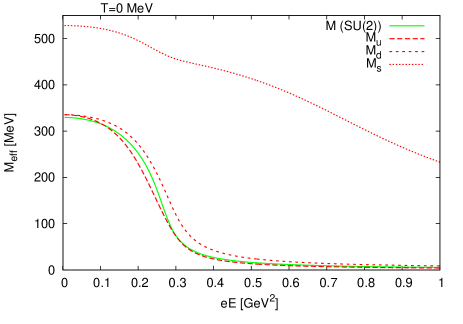
Figure 1: Effective quark masses as a function of the electric field for $T=0$.

We next consider the effect of the temperature on the effective quark masses. In Fig.2 the effective masses are plotted as a function of $eE$ at $T=130$MeV. One can see that the temperature has the effect to break the chiral condensates and just like electric field to weaken the constituent dynamical quark masses. In this way, we can see that when the temperature grows the pseudocritical electric field $eE_{c}$ decreases. The same analysis can be done in Fig.3 where we fix $T=200$MeV. Here we notice that just due to the effect of the temperature the chiral symmetry is almost completely restored and we can see a noticeable decrease of the pseudocritical electric field by the order $eE_{c}\sim 0.15$GeV².

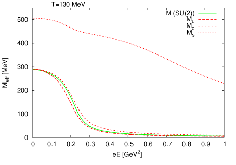
Figure 2: Effective quark masses as a function of the electric field for $T=130MeV$.

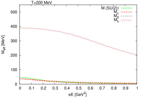
Figure 3: Effective quark masses as a function of the electric field for $T=200MeV$.

In Fig.4 we show the effect of finite chemical potential in the electrized quark matter for the SU(2) and SU(3) NJL models. In general, the chemical potential has the effect of partially restore the chiral symmetry, weakening the effective masses in both models at $eE=0$. Hence, we can expect the lowering of the critical electric field when the chemical potential increases. The effective masses of the lightest quarks have a similar behavior in both models, with a natural displacement in the SU(3) effective masses at $eE>0.1$GeV² due to the difference of the $u$ and $d$ quark electric charges and the strange quark effective mass is weakened as an effect of finite $\mu$.

In Fig.5, where the effective quark masses at $eE=0$ are plotted as a function of the temperature , the chiral symmetry restoration at finite temperature and zero electric field can be analyzed. One can see that the restoration occurs around $T_{c}\sim 200$MeV and the behavior of the SU(2) and SU(3) light masses are qualitatively the same.

The strange quark mass decreases more slowly, presenting a smooth bump at $T\sim 170$ MeV. In Fig.6 one can see that the effect of the inclusion of a electric field $eE=0.1$GeV² is to decrease the effective mass of the strange quark and cause a shift of the effective $u$ and $d$ quark masses with the $u$ quark mass becoming larger than the $d$ quark mass. One can observe that both the electric field and the temperature weaken the quark condensates, however, at sufficiently high temperatures the behavior of the lightest quark masses is qualitatively the same. In Fig.7, as an effect of a stronger electric field, one can see a larger shift of the lightest effective quark masses and a slightly smaller effective strange quark mass.

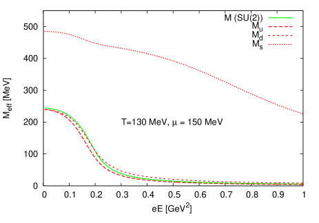
Figure 4: Effective quark masses as a function of the Electric Field for $T=130$MeV and $\mu=150$MeV.

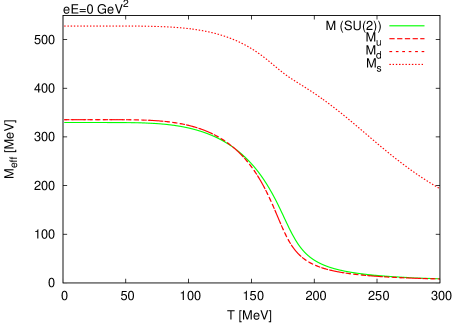
Figure 5: Effective quark masses as a function of the temperature for the electric field $eE=0$.

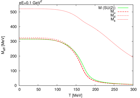
Figure 6: Effective quark masses as a function of the temperature for the electric field $eE=0.1$GeV².

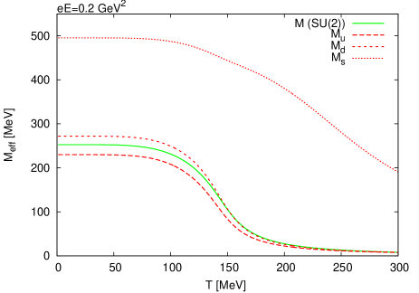
Figure 7: Effective quark masses as a function of the temperature for the electric field $eE=0.2$GeV².

From the figures 5,6,7 it is interesting to see that the (pseudocritical) temperature of the second order phase transition decreases with the increase of the electric field, so the electric field enhances the chiral symmetry restoration. As mentioned earlier, if we increase the electric field, the imaginary part of the effective potential becomes different of zero and we can associate this imaginary component to the creation of quark-antiquark pairs.

The Schwinger pair-production rate $\Gamma$ is shown in Fig.8 as a function of the electric field for the two versions of the NJL model at $T=0$ and $T=200$MeV. The results shows very little difference between both models at $T=0$ and after $eE\sim 0.2$GeV² the production rate grows more quickly due to the weakening of the chiral condensates and the QCD vacuum becomes more and more unstable and the pair of particle-antiparticle becomes more likely to happen. If we rises the temperature to $T=200$MeV, we can see almost no difference between the two models and the production rate increases considerably for electric fields $eE<0.3$GeV² when compared to the case $T=0$. The effect of finite chemical potential is shown in Fig.9, where we compare the production rate in both models with $\mu=0$ and $\mu=150$MeV at $T=130$MeV. The two versions of the NJL model agree in their general aspects, with quantitative differences in the transition region. As we can see the effect of finite chemical potential is to increase slightly the production rate at lower electric field.

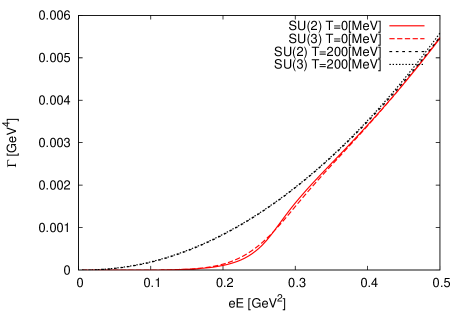
Figure 8: Schwinger Pair-Production as a function of the electric field for temperatures T=0 MeV and T=200 MeV.

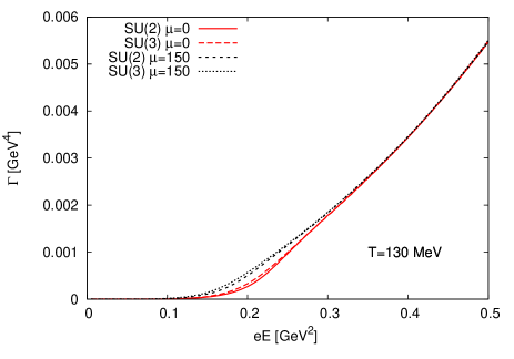
Figure 9: Schwinger Pair-Production as a function of the electric field at $T=130$ MeV and $\mu=0$ MeV and $\mu=150$ MeV.

In Fig.10 we show the Schwinger pair production as a function of the temperature at fixed electric fields $eE=0.1$GeV², $eE=0.2$GeV² and $eE=0.4$GeV². At $eE=0.1$GeV² we can see that the production rate grows quickly when a phase transition becomes more apparent at $T\sim 150$MeV, with a more prominent production rate for the SU(3) model in comparison to the SU(2) and stabilizes at $T\sim 200$MeV. This happens because the phase transition in this case is driven entirely by the temperature and when the chiral symmetry is partially restored we can expect the Schwinger pair production to become almost stable. If we increase the electric field to $eE=0.2$GeV², the production rate is more significant in the SU(3) model and when we reach $T\sim 100$MeV the production rate starts to increase more quickly and stabilize again, when for the two NJL models the Schwinger rate almost coincides. However, the production rate is more than four times greater than the production rate of $eE=0.1$GeV² case.

We also show our results for $eE=0.4$ GeV² since this value is approximately the electric field predicted in the simulationsdeng . For this electric field the chiral symmetry has already been partially restored and almost no quantitative difference is seen for $T<200$MeV in both models, but the effects of high temperatures are prominent in the SU(3) model where the production rate grows while in the SU(2) the production rate stabilizes.

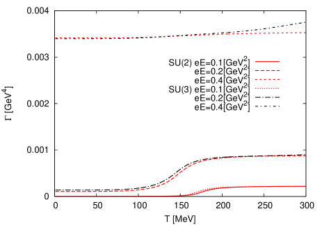
Figure 10: Schwinger Pair-Production rate as a function of the temperatures for the electric fields $eE=0.1$GeV², $eE=0.2$GeV² and $eE=0.4$GeV².

VI Conclusions

In this work we use the SU(2) and SU(3) versions of Nambu–Jona-Lasinio model at finite temperature and densities to study how a constant electric field in the $z$ direction can affect the chiral symmetry restoration. To this end, in the the SU(3) version we improve the calculations by including the ’t Hooft determinant in comparison withtatsumi and also assuming, differently from ref.(Cao ), non-zero current quark masses in both SU(2) and SU(3) models in order to calculate the effective quark masses and the Schwinger pair production.

The real part of the gap equation and of the effective potential should be properly regularized, since their $T=0$ contributions are divergent. We derive a set of regularized expressions obtained by analytical continuation in the Appendices of this work. These expressions are much more convenient to be used in numerical calculations, since avoids the highly-oscillatory integrals of eq.(5) and eq.(8)Cao ; ruggieri1 ; ruggieri2 ; tatsumi and as usual for the expressions at finite $T$ and $\mu$ we do not use any regularization since these integrals are finiteayala .

Firstly, we explore how the electric field restores the chiral symmetry. The general feature of the electric field is to the break the chiral condensates and in comparison to the SU(2) case, we can see a splitting of the dynamically generated masses of the $u$ and $d$ quarks $M_{u}$ and $M_{d}$ at relatively weak electric fields $eE\sim 0.1$GeV². For the strange quark, its effective mass $M_{s}$ decreases more slowly and the current quark mass $m_{s}$ is reached only at a very strong electric fields. The net effect is that the higher is the electric field the lower is the (pseudocritical) temperature of chiral restoration.

Analogously, the effect of the temperature is to enhance the chiral symmetry restoration and the higher the temperature the lower the corresponding electric field where the chiral symmetry is restored. The results for the Schwinger pair production evaluated in the SU(2) and SU(3) versions of the NJL model show similar behavior, at low temperatures and with the electric field rising, the production tends to increase when we cross a pseudocritical electric field and if we increase the temperature, the Schwinger pair production tends to initiates at lower electric fields. Besides, the inclusion of strange quark matter in this work indicates that the production of quark-antiquark pairs should be more pronounced when compared with the results of the SU(2) model.

Appendix A The Principal Value of $\overline{\theta}^{\mathcal{E}}_{f}$

To evaluate the Principal Value of $\overline{\theta}^{\mathcal{E}}_{f}$ as given in eq.(11), we will perform an analytical continuation from the closely related expression obtained in the framework of magnetized quark matter subjected to a constant magnetic field in the $z$ direction in the context of NJL model. In this way, we just start writing the well-known resultavancini2 ; andersen ; dunne

$$\overline{\theta}^{\beta}_{f}=-\frac{N_{c}}{8\pi^{2}}\int_{0}^{\infty}ds\frac{e^{-sM_{f}^{2}}}{s^{3}}\left[\beta_{f}s\coth(\beta_{f}s)-1-\frac{\beta_{f}^{2}}{3}\right]$$ (25)

$$= \frac{N_{c}\beta_{f}^{2}}{2\pi^{2}}\left[\zeta^{\prime}(-1,x_{f})-\frac{1}{2}(x_{f}^{2}-x_{f})\ln x_{f}+\right.$$

$$\left.\frac{x_{f}^{2}}{4}-\frac{1}{12}(1+\ln x_{f})\right]~{},$$

where $x_{f}=\frac{M_{f}^{2}}{2\beta_{f}}$ and $\beta_{f}=|q_{f}|B$. The duality between magnetic and electric fields can be seen through the replacement $eB\rightarrow-ieE$Cao ; kleva . Therefore, we perform this duality in eq.(25) through the prescription $x_{f}\rightarrow iy_{f}$

$$\overline{\theta}^{\mathcal{E}}_{f}=-\frac{N_{c}\mathcal{E}_{f}^{2}}{2\pi^{2}}\left[\zeta^{\prime}(-1,iy_{f})-\frac{1}{2}(-y_{f}^{2}-iy_{f})\ln(iy_{f})\right.$$

$$\left.-\frac{y_{f}^{2}}{4}-\frac{1}{12}(1+\ln(iy_{f}))\right]~{}.$$ (26)

Now the main difficulty is to evaluate $\zeta^{\prime}(-1,iy_{f})$, since the remaining terms are almost trivial to obtain. To proceed we use a convenient relation between the derivative of the Riemann zeta function and the logarithm of the gamma function, $\ln\Gamma$, quoted without proof in ref.dunne .

$$\zeta^{\prime}(-1,x)=\zeta^{\prime}(-1)-\frac{x}{2}(1-x)-\frac{x}{2}\ln 2\pi+\int_{0}^{x}dx^{\prime}\ln\Gamma(x^{\prime})~{}.$$ (27)

Next we sketch a proof of the latter expression. Firstly, we write

$$\frac{\partial\zeta^{\prime}(-1,x)}{\partial x}\equiv\left.\frac{\partial}{\partial x}\frac{\partial}{\partial z}\zeta(z,x)\right|_{z=-1}=\left.-\frac{\partial}{\partial z}z\zeta(z+1,x)\right|_{z=-1}~{},$$ (28)

where the last equality follows from the relationapostol

$$\frac{\partial}{\partial x}\zeta(z,x)=-z\zeta(z+1,x)~{}.$$

We now calculate the last derivative in eq.(28) and use the following equalitiesapostol

$$\zeta(0,x)=\frac{1}{2}-x~{}~{},~{}~{}\zeta^{\prime}(0,x)=\ln\Gamma(x)-\frac{1}{2}\ln(2\pi)~{},$$

thus obtaining the expression:

$$\frac{\partial\zeta^{\prime}(-1,x)}{\partial x}=\left(\frac{1}{2}-x\right)+\left[\ln\Gamma(x)-\frac{1}{2}\ln(2\pi)\right]~{}.$$

A simple integration of the latter equation yields

$$\zeta^{\prime}(-1,x)=\zeta^{\prime}(-1)-\frac{x}{2}(1-x)-\frac{x}{2}\ln 2\pi+\int_{0}^{x}dx^{\prime}\ln\Gamma(x^{\prime})~{},$$ (29)

with $\zeta^{\prime}(-1)=\frac{1}{12}-\ln(A)$, where $A=1.2814271291...$, the Glaisher–Kinkelin constantglaisher . To evaluate the integral that has been left in the last equation we need to invoke a representation of $\ln\Gamma(x)$boros

$$\ln\Gamma(x)=-\gamma_{E}x-\ln(x)+\sum_{k=1}^{\infty}\left[\frac{x}{k}-\ln(1+\frac{x}{k})\right],$$ (30)

where $\gamma_{E}$ is the Euler-Mascheroni constant. Integrating the latter equation over the variable $x$ from $0$ to $iy_{f}$, one obtains the analytical continued expression

$$\int_{0}^{iy_{f}}dx\ln\Gamma(x)=\frac{\gamma_{E}y_{f}^{2}}{2}+y_{f}\frac{\pi}{2}+\sum_{k=1}^{\infty}\left[-\frac{y_{f}^{2}}{2k}-\right.$$

$$\left.k\left(\frac{1}{2}\ln\left(1+\frac{y_{f}^{2}}{k^{2}}\right)-\frac{y_{f}}{k}\tan^{-1}\frac{y_{f}}{k}\right)\right]+$$

$$i\left\{-y_{f}\ln y_{f}+y_{f}\right.$$

$$\left.-\sum_{k=1}^{\infty}\left[k\left(\frac{y_{f}}{2k}\ln\left(1+\frac{y_{f}^{2}}{k^{2}}\right)+\tan^{-1}\frac{y_{f}}{k}\right)-y_{f}\right]\right\}.$$ (31)

From eqs.(26,29,31) the analytically continued expression as given in eq.(18) can be straightforwardly obtained.

Appendix B The Principal Value of $\overline{\phi}_{f}^{\mathcal{E}}$

Next, we apply the same analytical continuation technique of the previous appendix in order to derive the principal value of the quark condensates. We use the SU(3) NJL condensates in a magnetic field taken from the literaturenosso1 ; avancini2 . To this end, we start from the regularized part of the condensate in a magnetic field

$$\overline{\phi}^{\beta}_{f}=-\frac{N_{c}M_{f}}{4\pi^{2}}\beta_{f}\int_{0}^{\infty}ds\frac{e^{-sM_{f}^{2}}}{s}\left[\coth(\beta_{f}s)-1\right]$$

$$=-\frac{N_{c}M_{f}}{2\pi^{2}}\beta_{f}\left[\ln\Gamma(x_{f})-\frac{1}{2}\ln(2\pi)\right.$$

$$\left.+x_{f}-\frac{1}{2}\left(x_{f}-1\right)\ln(x_{f})\right].$$ (32)

So, performing the analytic continuation of the latter equation, we can write the dual expression for the condensate, $\overline{\phi}^{\mathcal{E}}_{f}$, in a constant electric field in the $z$ direction as

$$\overline{\phi}^{\mathcal{E}}_{f}=\frac{-iN_{c}M_{f}}{4\pi^{2}}\mathcal{E}_{f}\int_{0}^{\infty}ds\frac{e^{-sM_{f}^{2}}}{s}\left[\coth(-i\mathcal{E}_{f}s)-1\right]$$

$$=-\frac{M_{f}N_{c}}{2\pi^{2}}i\mathcal{E}_{f}\left[\ln\Gamma(iy_{f})-\frac{1}{2}\ln(2\pi)\right.$$

$$\left.+iy_{f}-\frac{1}{2}\left(iy_{f}-1\right)\ln(iy_{f})\right].$$ (33)

We are interested in the real part of the eq.(B). Since $\coth(-ix)=i\cot(x)$, we have

$$\Re(\overline{\phi}^{\beta}_{f})=\Re\left\{\frac{N_{c}M_{f}}{4\pi^{2}}\mathcal{E}_{f}\int_{0}^{\infty}ds\frac{e^{-sM_{f}^{2}}}{s}\left[\cot(\mathcal{E}_{f}s)-1\right]\right\}$$

$$=-\frac{N_{c}M_{f}}{2\pi^{2}}\mathcal{E}_{f}\Re\left[i\ln\Gamma(iy_{f})-i\frac{1}{2}\ln(2\pi)+\right.$$

$$\left.-y_{f}-i\frac{1}{2}\left(iy_{f}-1\right)\ln(iy_{f})\right]~{}.$$ (34)

The imaginary part of $\ln\Gamma(x)$ can be extracted from its series representation given by eq.(30). If $z=|z|e^{i\theta}$ is an arbitrary complex number, its logarithm is given by $\ln z=\ln|z|+i\theta$. Using this expression one easily obtains:

$$\ln(1+i\frac{x}{k})=\frac{1}{2}\ln\left(1+\frac{x^{2}}{k^{2}}\right)+i\tan^{-1}\frac{x}{k}~{},$$ (35)

from the latter equation it follows that:

$$\Im\left[\ln(1+i\frac{y_{f}}{k})\right]=\tan^{-1}\frac{y_{f}}{k}~{}.$$

After substituting the last equation in eq.(30), it is straightforward to show that:

$$\Im\left(\ln\Gamma(iy_{f})\right)=-\gamma_{E}y_{f}-\frac{\pi}{2}+\sum_{k=1}^{\infty}\left[\frac{y_{f}}{k}-\tan^{-1}(\frac{x}{k})\right]~{},$$ (36)

The imaginary part of the eq.(B) can now easily be obtained, hence, the desired eq.(19) can be derived.

Appendix C Derivation of the Schwinger pair production rate $\Gamma$

We have to extract the imaginary part of the effective potential in order to obtain the Schwinger pair production rate, eq.(10).Since we wish to evaluate the imaginary part of $\theta^{\mathcal{E}}_{f}$, the term proportional to $\mathcal{E}^{2}$ can be discarded, and the eq.(8) should be given by

$$\overline{\theta}_{f}^{\mathcal{E}}=-\frac{N_{c}}{8\pi^{2}}\int_{0}^{\infty}ds\frac{e^{-sM_{f}^{2}}}{s^{3}}\left[\mathcal{E}_{f}s\cot(\mathcal{E}_{f}s)-1\right].$$ (37)

We now use the following trigonometric relation remment

$$\pi\cot(\pi x)=\frac{1}{x}+\sum_{k=1}^{\infty}\frac{2x}{x^{2}-k^{2}},$$ (38)

in eq.(37). After an appropriate change of variable, one obtains

$$\overline{\theta}_{f}^{\mathcal{E}}=-\frac{N_{c}}{8\pi^{4}}\mathcal{E}_{f}^{2}\int_{0}^{\infty}ds\frac{e^{-s\frac{\pi M_{f}^{2}}{\mathcal{E}_{f}}}}{s^{3}}\left(\sum_{k=1}^{\infty}\frac{2s^{2}}{s^{2}-k^{2}}\right).$$ (39)

Next, performing a simple partial fraction decomposition and using the identity $\lim_{\epsilon\rightarrow 0}\frac{1}{x\pm i\epsilon}=P.V\frac{1}{x}\mp i\pi\delta(x)$, we obtain

$$\Im({\overline{\theta}_{f}^{\mathcal{E}}})=\frac{N_{c}}{8\pi}\mathcal{E}_{f}^{2}\sum_{k=1}^{\infty}\frac{e^{-k\frac{\pi M_{f}^{2}}{\mathcal{E}_{f}}}}{(\pi k)^{2}},$$ (40)

plugging this result in the usual definition of the Schwinger pair-production rateSchwinger ; Cao , $\Gamma=-2\Im{(\Omega)}$, we obtain eq.(10).

Appendix D Equivalence between the imaginary part of eq.(26) and eq.(40)

Making use of eq.(26,29) and a change of variables $x^{\prime}=ix$ in the integration, the full imaginary part of the effective potential is given by

$$\Im{(\overline{\theta}^{\mathcal{E}}_{f})} = -\frac{N_{c}\mathcal{E}_{f}^{2}}{2\pi^{2}}\left[\Re\int_{0}^{y_{f}}dx\ln\Gamma(ix)-\frac{y_{f}}{2}-\frac{y_{f}}{2}\ln(2\pi)\right.$$ (41)

$$+ \frac{y_{f}}{2}\ln y_{f}\left.-\frac{y_{f}}{2}-\frac{y_{f}}{2}\ln(2\pi)+\frac{\pi}{4}y_{f}^{2}-\frac{\pi}{24}\right].$$

Now, to proceed we have to integrate $\ln\Gamma(x)$. First, we make use of the property $x\Gamma(x)=\Gamma(x+1)$, to obtain

$$\Re\int_{0}^{y_{f}}dx\ln\Gamma(ix)=\Re\left[\int_{0}^{y_{f}}dx\ln\Gamma(1+ix)-\int_{0}^{y_{f}}dx\ln(ix)\right],$$ (42)

the second integration is trivial, and is given by

$$\int_{0}^{y_{f}}dx\ln(ix)=y_{f}(\ln y_{f}-1)+\frac{i\pi}{2}y_{f}.$$ (43)

By using the formulas of referencesgrad ; dittrich

$$\Re\left[\ln\Gamma(1+ix)\right] =\frac{1}{2}\ln|\Gamma(1-ix)\Gamma(1+ix)|$$

$$=-\frac{1}{2}\ln\frac{\sinh(\pi x)}{\pi x},$$

and performing an integration by parts, the first integral in eq.(42) can be solved

$$\Re\left[\int_{0}^{y_{f}}dx\ln\Gamma(1+ix)\right]=-\frac{1}{2}\left\{y_{f}\ln\frac{\sinh(\pi y_{f})}{\pi y_{f}}\right.$$ (45)

$$\left.-\int_{0}^{y_{f}}dx\left[\pi x\coth(\pi x)-1\right]\right\},$$

performing of variables $\pi x=z$ and the following resultdittrich

$$\frac{1}{\pi}\int_{0}^{y_{f}\pi}dzz\coth(z)=\frac{1}{2\pi}\left[-(y_{f}\pi)^{2}+2y_{f}\pi\ln(2)\right.$$ (46)

$$\left.+2y_{f}\pi\ln\sinh(\pi y_{f})-Li_{2}(e^{-2y_{f}\pi})+Li_{2}(1)\right],$$

where $Li_{2}(x)=\sum_{k=1}^{\infty}\frac{x^{k}}{k^{2}}$ is the Polylogarithm function of order 2 and we also use the very famous result $Li_{2}(1)=\frac{\pi^{2}}{6}$. Using these results, all the remaining terms of eq.(41) cancel each other, remaining only

$$\Im{(\overline{\theta}^{\mathcal{E}}_{f})}=-\frac{N_{c}\mathcal{E}_{f}^{2}}{2\pi^{2}}\left[-\frac{1}{4\pi}Li_{2}(e^{-2y_{f}\pi})\right]$$ (47)

$$=\frac{N_{c}\mathcal{E}_{f}^{2}}{8\pi}\sum_{k=1}^{\infty}\frac{e^{-k\frac{M_{f}^{2}\pi}{\mathcal{E}_{f}}}}{(\pi k)^{2}}.$$ (48)

References

- (1) H. Heiselberg and M. Hjorth-Jensen,” Phys. Rept.328, 237 (2000), arXiv:nucl-th/9902033.
- (2) K. Yagi, T. Hatsuda and Y. Miake, Part. Phys. Nucl. Phys. Cosmol. 23, 1 (2005).
- (3) T. Vachaspati, Phys. Lett. B 265, 258 (1991).
- (4) S. Muroya, A. Nakamura, C. Nonaka, and T. Takaishi, Prog. Theor. Phys. 110, 615 (2003), arXiv:hep-lat/0306031.
- (5) K. Fukushima and T. Hatsuda, Rept. Prog. Phys. 74, 014001 (2011).
- (6) K. Fukushima, D. E. Kharzeev and H. J. Warringa, Phys. Rev. D 78, 074033, (2008); D. E. Kharzeev and H. J. Warringa, Phys. Rev. D 80, 034028 (2009); D. E. Kharzeev, Nucl. Phys. A 830, 543c (2009).
- (7) R. Duncan and C. Thompson, Astron. J., 32, L9 (1992);
- (8) C. Kouveliotou et al., Nature 393, 235 (1998).
- (9) V. A. Miransky and I. A. Shovkovy, arXiv:1503.00732 [hep-ph]; D. Ebert, K. G. Klimenko, M. A. Vdovichenko, and A. S. Vshivtsev, Phys. Rev. D 61, 025005 (1999), arXiv:hep-ph/9905253; K. G. Klimenko, Z. Phys. C 54, 323 (1992); K. G. Klimenko, arXiv:hep-ph/9809218.
- (10) T. Hatsuda and T. Kunihiro, Phys. Rep. 247, 221 (1994).
- (11) D. P. Menezes, M. Benghi Pinto, S. S. Avancini, A. Pérez Martínez, and C. Providência, Phys. Rev. C 79, 035807 (2009).
- (12) D. P. Menezes, M. Benghi Pinto, S. S. Avancini, and C. Providência, Phys. Rev. C 80, 065805 (2009).
- (13) G. Bali, F. Bruckmann, G. Endrodi, Z. Fodor, S. Katz, S. Krieg, A. Schäfer, and K. K. Szabó, J. High Energy Phys. 02 (2012) 044; G. Bali, F. Bruckmann, G. Endrodi, Z. Fodor, S. Katz, and A. Schäfer, Phys. Rev. D 86, 071502 (2012).
- (14) A. Bzdak and V. Skokov, Phys. Lett. B 710, 171 (2012).
- (15) W. T. Deng and X. G. Huang, Phys. Rev. C 85, 044907 (2012)
- (16) J. Bloczynski, X. G. Huang, X. Zhang, and J. Liao, Phys. Lett. B 718, 1529 (2013).
- (17) J. Bloczynski, X. G. Huang, X. Zhang, and J. Liao, Nucl. Phys. A 939, 85 (2015).
- (18) Y. Hirono, M. Hongo, and T. Hirano, Phys. Rev. C 90, 021903(R) (2014).
- (19) V. Voronyuk, V. D. Toneev, S. A. Voloshin, and W. Cassing, Phys. Rev. C 90, 064903 (2014).
- (20) W. T. Deng and X. G. Huang, Phys. Lett. B 742, 296 (2015), arXiv:1411.2733 [nucl-th].
- (21) G. Cao and X. G. Huang, Phys. Rev. D 93, 016007 (2016).
- (22) M. Ruggieri, Z.Y. Lu, and G.X.Peng, Phys. Rev. D 94, 116003 (2016).
- (23) M. Ruggieri and G.X. Peng, Phys. Rev. D 93, 094021 (2016).
- (24) S. P. Klevansky, Rev. Mod. Phys. 64, 649 (1992); S. P. Klevansky and R. H. Lemmer, Phys. Rev. D 39, 3478 (1989).
- (25) B. C. Tiburzi, Nucl. Phys. A 814, 74 (2008), arXiv:0808.3965 [hep-ph].
- (26) A. Yamamoto, Phys. Rev. Lett. 110, 112001 (2013).
- (27) A. Y. Babansky, E. V. Gorbar, and G. V. Shchepanyuk, Phys. Lett. B 419, 272 (1998).
- (28) T. D. Cohen, D. A. McGady, and E. S. Werbos, Phys. Rev. C 76, 055201 (2007).
- (29) G. Cao and X. G. Huang, Phys. Lett. B 757, 1 (2016).
- (30) H. Suganuma, T. Tatsumi, Chiral Symmetry and Quark-Antiquark Pair Creation in a Strong Color-Electromagnetic Field, Progress of Theoretical Physics, Volume 90, Issue 2, 1 August 1993, Pages 379–404.
- (31) X. G. Huang and J. Liao, Phys. Rev. Lett. 110, 232302 (2013).
- (32) Y. Jiang, X. G. Huang, and J. Liao, Phys. Rev. D 91, 045001 (2015).
- (33) J. S. Schwinger, Phys. Rev. 82, 664 (1951).
- (34) W. Heisenberg and H. Euler, Z. Phys. 98, 714 (1936).
- (35) Y. Nambu and G. Jona-Lasinio, Phys. Rev. 122, 345 (1961); 124, 246 (1961).
- (36) M. Buballa, Phys. Rep. 407, 205 (2005).
- (37) A. Ayala, C. A Dominguez, L. A. Hernández, M. Loewe, A. Raya, J. C. Rojas, and C. Villavicencio, Phys. Rev. D 94, 054019 (2016).
- (38) I. S. Gradshteyn and I. M. Ryzhik, Tables of Integrals, series and Products,Academic Press, USA, 1980.
- (39) J. O. Andersen, W. R. Naylor and A. Tranberg , Rev. Mod. Phys. 88, 025001 (2016), arXiv:hep-ph/1411.7176.
- (40) G. V. Dunne,“ From Fields to Strings: Circumnavigating Theoretical Physics, Ian Kogan Memorial Collection”, Eds. M. Shifman, A. Vainshtein and J. Wheater, World Scientific, 2004, arXiv:hep-th/0406216.
- (41) T. M. Apostol, in “NIST Handbook of Mathematical Functions”, Cambridge University Press, New York, 2010.
- (42) Glaisher, J. W. L. Messenger Math. 7, 43 (1878).
- (43) Boros, G. and Moll, V. ”The Expansion of the Loggamma Function.” §10.6 in Irresistible Integrals: Symbolics, Analysis and Experiments in the Evaluation of Integrals. Cambridge, England: Cambridge University Press, pp. 201-203, 2004.
- (44) Remmert, Reinhold (1991). Theory of complex functions. Springer. p. 327. ISBN 0-387-97195-5. Extract of page 327.
- (45) W. Dittrich, Int. J. Mod. Phys. A, 29, 1430033 (2014).