A Distribution-Free Test of Independence and Its Application to Variable Selection

Abstract

Motivated by the importance of measuring the association between the response and predictors in high dimensional data, we propose a new distribution-free test of independence between a categorical response variable $Y$ and a continuous predictor $X$ based on mean variance (MV) index. The mean variance index can be considered as the weighted average of Cramér-von Mises distances between the conditional distribution functions of $X$ given each class of $Y$ and the unconditional distribution function of $X$. The mean variance index is zero if and only if $X$ and $Y$ are independent. In this paper, we propose a new MV test between $X$ and $Y$ and it enjoys several appealing merits. First, under the independence between $X$ and $Y$, we derive an explicit form of the asymptotic null distribution, $\sum_{j=1}^{+\infty}{\chi_{j}^{2}(R-1)}/{\pi^{2}j^{2}}$, where $\chi_{j}^{2}(R-1),j=1,2,\ldots$, are independent $\chi^{2}$ random variables with $R-1$ degrees of freedom and $R$ is the fixed number of classes of $Y$. It provides us with an efficient and fast way to compute the empirical p-value in practice. Second, we can allow $R$ diverge slowly to the infinity as the sample size increases and the limiting null distribution of the standardized test statistic is a standard normal distribution. Third, it is essentially a rank test and thus distribution-free. No assumption on the distributions of two random variables is required and the test statistic is invariant under one-to-one transformations. It is resistant to heavy-tailed distributions and extreme values in practice. We assess its excellent performance by Monte Carlo simulations. As its important application, we apply the MV test to high dimensional colon cancer gene expression data to detect the significant genes associated with the tissue syndrome.

Running Head: A Distribution-Free Test of Independence

Key words: Asymptotic null distribution, conditional distribution function, mean variance index, high dimensional data, test of independence, variable selection.

1 Introduction

One of the fundamental goals of data analysis and statistical inference is to understand the relationship among random variables. In many scientific researches, it is of importance and interest to test whether two random variables are statistically independent of one another. Many real-life examples can be found in finance, physics, biology and medical science, etc. For instance, the genetics researchers may be interested in testing the independence between some inherited disease and a single-nucleotide polymorphism (SNP) or whether two groups of genes are associated in high dimensional genetic data. The medical researchers may want to understand the relationship between the lung cancer and the smoking status.

As a fundamental statistical problem, testing whether two random variables are independent or not has received much attention in the literature. When two random variables are both categorical, the classic Pearson’s chi-square test is applied to test their statistical independence. Note that the independence of two random variables $X$ and $Y$ is equivalent to $H_{0}:F_{XY}=F_{X}F_{Y}$, where $F_{XY}$ denotes the joint distribution function of $(X,Y)$ and $F_{X}$ and $F_{Y}$ denote the marginal distributions of $X$ and $Y$, respectively. Hoeffding (1948) proposed a test of independence based on the difference between the joint distribution function and the product of marginals. The Hoeffding’s test statistic is

$$H_{n}=n\int\int\left[\hat{F}_{XY}(x,y)-\hat{F}_{X}(x)\hat{F}_{Y}(y)\right]^{2}d\hat{F}_{XY}(x,y),$$ (1.1)

where $\hat{F}$ denotes the empirical distribution function. This is also the well-known Cramér-von Mises criterion between the joint distribution function and the product of marginals. Rosenblatt (1975) considered a measure of dependence based on the difference between the joint density function and the product of marginal densities. To consider the quadratic distance between the joint characteristic function and the product of the marginal characteristic functions, Szekely, Rizzo and Bakirov (2007) and Szekely and Rizzo (2009) defined a distance covariance (DC) between two random vectors $X\in\mathbb{R}^{p}$ and $Y\in\mathbb{R}^{q}$ by

$$V^{2}(X,Y)=\int_{\mathbb{R}^{p+q}}\left|\phi_{XY}(t,s)-\phi_{X}(t)\phi_{Y}(s)\right|^{2}\omega(t,s)dtds,$$ (1.2)

where $\phi_{XY}(t,s),\phi_{X}(t),\phi_{Y}(s)$ denote the joint characteristic function, the marginal characteristic functions of $X$ and $Y$, respectively, and $\omega(t,s)$ is a positive weight function. $V^{2}(X,Y)=0$ if and only if $X$ and $Y$ are independent. They further proposed a test of independence based on the statistic $nV^{2}_{n}(X,Y)/S_{2}$, where $V^{2}_{n}(X,Y)$ is the estimator for $V^{2}(X,Y)$ by using the corresponding empirical characteristic functions and $S_{2}=n^{-4}\sum_{k,l=1}^{n}|X_{k}-X_{l}|_{p}\sum_{k,l=1}^{n}|Y_{k}-Y_{l}|_{q}$ in which $\{(X_{i},Y_{i}),i=1,2,\ldots,n\}$ is a random sample of $(X,Y)$. Under the existence of moments, it was proved that $nV^{2}_{n}(X,Y)/S_{2}$ converges in distribution to a quadratic form $\sum_{j=1}^{+\infty}\lambda_{j}Z_{j}^{2}$, where $Z_{j}$ are independent standard normal random variables and the values of $\lambda_{j}$ depend on the distribution of $(X,Y)$. Recently, Heller, Heller and Corfine (2013) developed a consistent multivariate test of association based on ranks of distances. Bergsma and Dassios (2014) proposed another consistent test of independence based on a sign covariance related to Kendall’s tau.

In this paper, we propose a novel distribution-free test for the independence between a categorical random variable and a continuous one based on mean variance (MV) index. It is important to understand the relationship between a categorical variable and a continuous one in practice, such as the relationship between the SNP and a continuous genetic trait, the tumor class and gene expression levels (continuous), or the social status and the family income, etc. Let $Y$ be a categorical variable with $R$ classes $\{y_{1},y_{2},\ldots,y_{R}\}$, and $X$ be a continuous variable. The MV index can be considered as the weighted average of Cramér-von Mises distances between the conditional distribution functions of $X$ given each $Y=y_{r}$ and the unconditional distribution function of $X$. Note that the MV index equals to 0 if and only if $X$ and $Y$ are statistically independent. Thus, the MV index can be used to construct a test statistic for independence. The proposed MV test enjoys several advantages. (1) Under the null hypothesis of independence between two variables, the asymptotic null distribution has an explicit form when $R$ is fixed. That is, $\sum_{j=1}^{+\infty}{\chi_{j}^{2}(R-1)}/{\pi^{2}j^{2}}$, where $\chi_{j}^{2}(R-1),j=1,2,\ldots$, are independent $\chi^{2}$ random variables with $R-1$ degrees of freedom. It provides us with an efficient and fast way to compute the critical value and make a test decision quickly in practice. (2) The number of classes $R$ can be allowed to approach infinity with the sample size $n$ at a relatively slow rate. The limiting null distribution of the standardized MV statistic is a standard normal distribution. It is convenient to obtain any critical value in practice using an approximated normal distribution when $R$ is large. (3) The proposed test is essentially a rank test and thus distribution-free. Thus, the MV test statistic is invariant for any fixed $n$ under one-to-one transformations and resistent to heavy-tailed distributions and extreme values in practice. Numerical studies show that the MV test has a higher or comparable power performance compared with the existing methods even when $X$ is generated from a standard Cauchy distribution. Furthermore, there is no distribution assumption required to derive the asymptotic null distributions. This merit is not shared by the distance covariance test (Szekely, Rizzo and Bakirov, 2007) whose asymptotic null distribution depends on the distribution of $(X,Y)$ and has no explicit form.

The rest of this paper is organized as follows. In Section 2, we introduce the mean variance index and its properties. Main results are included in Section 3, where we will propose a new distribution-free MV test and derive its asymptotic distributions. In Section 4, we study the power performance of the new test compared with the existing alternative methods using Monte Carlo simulations and a real-data application. Section 5 discusses some extensions. Technical proofs are given in the Appendix.

2 Mean Variance Index

In this section, we briefly introduce the mean variance index defined for a continuous random variable and a categorical one. Let $X$ be a continuous random variable with a support $\mathbb{R}_{X}$ and $Y$ be a categorical random variable with $R$ classes $\{y_{1},y_{2},\ldots,y_{R}\}$. The mean variance (MV) index of $X$ given $Y$ defined in Cui, Li and Zhong (2015) by

$$MV(X|Y)=E_{X}[Var_{Y}(F(X|Y))],$$ (2.1)

where $F(x|Y)=\mathbb{P}(X\leq x|Y)$ denotes the conditional distribution function of $X$ given $Y$. We further let $F(x)=\mathbb{P}(X\leq x)$ denote the unconditional distribution function of $X$, and $F_{r}(x)=\mathbb{P}(X\leq x|Y=y_{r})$ be the conditional distribution function of $X$ given $Y=y_{r}$. Cui, Li and Zhong (2015) showed that $MV(X|Y)$ can be represented as the following quadratic form between $F(x)$ and $F_{r}(x)$,

$$MV(X|Y)=\sum_{r=1}^{R}p_{r}\int\left[F_{r}(x)-F(x)\right]^{2}dF(x),$$ (2.2)

where $p_{r}=\mathbb{P}(Y=y_{r})>0$ for all $r=1,\ldots,R$. It is worth noting that $MV(X|Y)$ can be considered as the weighted average of Cramér-von Mises distances between the conditional distribution functions of $X$ given each $Y=y_{r}$ and the unconditional distribution function of $X$. This observation further implies the following Lemma.

Lemma 2.1.

$MV(X|Y)=0$ if and only if $X$ and $Y$ are statistically independent.

Lemma 2.1 indicates that the MV index $MV(X|Y)$ can measure any dependence between a continuous random variable and a categorical one. Due to this property, we will propose a test of independence between $X$ and $Y$ based on their MV index and develop the associated asymptotic distributions in the later section.

Next, we provide a consistent estimator for $MV(X|Y)$. Suppose that $\{(X_{i},Y_{i}):i=1,\ldots,n\}$ with the sample size $n$ is randomly drawn from the population distribution of $(X,Y)$. Using the idea of method of moments, $MV(X|Y)$ can be estimated by the following statistic

$$\widehat{MV}(X|Y)=\frac{1}{n}\sum_{r=1}^{R}\sum_{i=1}^{n}\hat{p}_{r}\left[\hat{F}_{r}(X_{i})-\hat{F}(X_{i})\right]^{2},$$ (2.3)

where $\hat{F}(x)=n^{-1}\sum_{i=1}^{n}I\{X_{i}\leq x\}$ is the empirical unconditional distribution function of $X$, $\hat{F}_{r}(x)=\sum_{i=1}^{n}I\{X_{i}\leq x,Y_{i}=y_{r}\}/\sum_{i=1}^{n}I\{Y_{i}=y_{r}\}$ is the empirical conditional distribution function of $X$ given $Y=y_{r}$, and $\hat{p}_{r}=n^{-1}\sum_{i=1}^{n}I\{Y_{i}=y_{r}\}$ denotes the sample proportion of the $r$th class, where $I\{\cdot\}$ represents the indicator function. The following lemma demonstrates the consistency of the proposed estimator for $MV(X|Y)$, which is the direct corollary of Theorem 2.1 in Cui, Li and Zhong (2015).

Lemma 2.2.

Suppose $R=R(n)=O(n^{\kappa})$ for some $0\leq\kappa<1$ and there exist two positive constants $c_{1}$ and $c_{2}$ such that $\displaystyle c_{1}/R\leq\underset{1\leq r\leq R}{\min}p_{r}\leq\underset{1\leq r\leq R}{\max}p_{r}\leq c_{2}/R$. Then, for any $\epsilon\in(0,1/2)$, there exists a positive constant $c>0$ such that

$$~{}~{}~{}~{}\mathbb{P}\left\{\left|\widehat{MV}(X|Y)-MV(X|Y)\right|\geq\epsilon\right\}\leq O(n)R\exp\left\{-\frac{cn}{R}\epsilon^{2}\right\}\rightarrow 0,$$ (2.4)

as $n\rightarrow\infty$. That is, $\widehat{MV}(X|Y)\overset{p}{\rightarrow}MV(X|Y)$, as $n\rightarrow\infty$. Hence, $\widehat{MV}(X|Y)$ is consistent to the mean variance index $MV(X|Y)$.

Remark: The condition $\displaystyle c_{1}/R\leq\underset{1\leq r\leq R}{\min}p_{r}\leq\underset{1\leq r\leq R}{\max}p_{r}\leq c_{2}/R$ requires that the proportion of each class of $Y$ cannot be either too small or too large as $n$ increases. Here, $R=O(n^{\kappa})$ is allowed to be diverging at a relatively slow rate of the sample size $n$. If $R$ is fixed when $\kappa=0$, the condition $\displaystyle c_{1}/R\leq\underset{1\leq r\leq R}{\min}p_{r}\leq\underset{1\leq r\leq R}{\max}p_{r}\leq c_{2}/R$ is automatically satisfied and the result also holds.

3 Main Results

3.1 Mean Variance Test of Independence

In this section, we will present a distribution-free test of independence between a continuous random variable $X$ and a categorical one $Y$ based on their mean variance index. We consider the following testing hypothesis:

$$H_{0}:\mbox{$X$ and $Y$ are statistically independent.}$$

versus $$H_{1}:\mbox{$X$ and $Y$ are not statistically independent.}$$

Note that the null hypothesis is equivalent to that the conditional distribution function of $X$ given $Y=y_{r}$ is always equal to the unconditional distribution function $X$ for any $r=1,\ldots,R$. That is, $F_{r}(x)=F(x)$. Thus, the previous hypothesis can be rewritten as

$$H_{0}:F_{r}(x)=F(x)\mbox{~{}for any~{}}x\mbox{~{}and~{}}r=1,\ldots,R.$$

versus $$H_{1}:F_{r}(x)\neq F(x)\mbox{~{}for some~{}}x\mbox{~{}and~{}}r=1,\ldots,R.$$

To test $H_{0}$, we naturally consider the difference between each $F_{r}(x)$ and $F(x)$. Note that the proposed MV index (2.2) is the weighted quadratic distance between $F_{r}(x)$’s and $F(x)$ with the proportion of each class as weights. Therefore, we propose a new test statistic based on the sample-level MV index

$$T_{n}=n\widehat{MV}(X|Y)=\sum_{r=1}^{R}\sum_{i=1}^{n}\hat{p}_{r}\left[\hat{F}_{r}(X_{i})-\hat{F}(X_{i})\right]^{2}.$$ (3.1)

The larger value of $T_{n}$ provides a stronger evidence against the null hypothesis $H_{0}$. We name the new test as the Mean Variance (MV) Test of independence.

Before studying its theoretical properties of the MV test, we run a simple simulation example to get a first insight into how it performs. Let us generate a random variable $X$ from a standard normal distribution and random variables $Z_{k}$ with $k=0,1,2$ by $Z_{0}=\varepsilon$, $Z_{1}=X+\varepsilon$ and $Z_{2}=2X^{2}+\varepsilon,$ where $\varepsilon\sim N(0,1)$ independent of $X$. For each $k=0,1,2$, let $Y_{k}=I(Z_{k}\leq q_{k1})+2I(q_{k1}<Z_{k}\leq q_{k2})+3I(q_{k2}<Z_{k}\leq q_{k3})+4I(Z_{k}>q_{k3}),$ where $\{q_{k1},q_{k2},q_{k3}\}$ are the first, second and third quartiles of $Z_{k}$, respectively. Thus, $Y_{0}$ is statistically independent of $X$ while $Y_{1}$ and $Y_{2}$ respectively depend on $X$ through a linear term and a quadratic term, respectively. We consider the sample sizes $n$ from 20 to 150. For a given sample size, $T_{n}$ is computed for each pair of $(X,Y_{k})$ and the associated p-value is also calculated using its limiting null distribution which will be given in (3.2). We conduct this simulation 100 times to compute the empirical powers or type-I error rates (if $H_{0}$ is true) at the nominal significance level 0.05. The left panel of Figure 1 depicts the mean of MV test statistic values against the sample sizes. When $X$ and $Y_{0}$ are independent, the values of $T_{n}$ are close to zero for all of the sample sizes. However, the values of $T_{n}$ increase substantially as the sample sizes increase when $Y_{k}$ is dependent on $X$, for $k=1,2$. The right panel displays the empirical powers of MV test of independence against the sample sizes. When $H_{0}$ is true, i.e. $X$ and $Y_{0}$ are independent, the dotted line shows the empirical type-I error rates for different samples sizes. The MV test performs well because the empirical type-I error rates are close to $0.05$ and have mean 0.048 and standard deviation 0.016. When $H_{0}$ is false, the empirical powers increase quickly to 1 as the sample size increases. It indicates that the MV test is useful against both linear and quadratic dependence alternatives between a categorical random variable and a continuous one. More numerical studies can be seen in Section 4.

Figure 1: The left panel depicts the MV test statistic values against the sample sizes and the right panel displays the empirical powers of MV test of independence against the sample sizes. In the both panels, the dotted line, the dashed line and the solid line denote the tests of independence between $(X,Y_{0})$, $(X,Y_{1})$ and $(X,Y_{2})$, respectively.

3.2 Asymptotic Distributions of MV Test Statistic

As aforementioned, the MV test statistic $T_{n}$ has a simple form and is easy to calculate and interpret. However, it is by no means straightforward to derive its asymptotic distributions. In this subsection, we will study the asymptotic distributions of $T_{n}$ with the aid of the empirical processes theory.

First of all, we derive the asymptotic null distribution of $T_{n}$ when the class number $R$ is fixed. The proof is given in the Appendix.

Theorem 3.1.

Suppose $X$ is a continuous random variable and $Y$ is a categorical random variable with a fixed number $R$ of classes. Under $H_{0}$,

$$T_{n}=n\widehat{MV}(X|Y)\overset{d}{\longrightarrow}\sum_{j=1}^{+\infty}\frac{\chi_{j}^{2}(R-1)}{\pi^{2}j^{2}},$$ (3.2)

where $\chi_{j}^{2}(R-1)$’s, $j=1,2,\cdots$, are independently and identically distributed (i.i.d.) $\chi^{2}$ random variables with $R-1$ degrees of freedom, and $\overset{d}{\longrightarrow}$ denotes the convergence in distribution.

Theorem 3.1 demonstrates the appealing advantages of the proposed MV test. First of all, under the independence between $X$ and $Y$, the asymptotic null distribution has an explicit quadratic form $\sum_{j=1}^{+\infty}{\chi_{j}^{2}(R-1)}/{\pi^{2}j^{2}},$ which provides us with an efficient way to compute the empirical p-value and draw a test conclusion in practice. It is very helpful especially when both the number of tests to conduct and the sample size are very large. Second, the MV test is essentially a rank test and thus distribution-free because the test statistic is only based on the empirical distribution functions. There is no assumption on the distribution of $X$ or $Y$ required to prove Theorem 3.1 and the MV test statistic is invariant under any one-to-one transformation. This merit makes the MV test have a wide range of applications. The distance covariance test does not share this feature because its asymptotic null distribution depends on the distribution of $(X,Y)$.

Remark: This theoretical result is related to the asymptotic null distributions of some tests in the literature. Szekely, Rizzo and Bakirov (2007) proved that the asymptotic null distribution of their distance covariance test statistic also has a quadratic form $\sum_{j=1}^{+\infty}\lambda_{j}Z_{j}^{2}$ where $Z_{j}$’s are independent standard normal random variables, but the values of $\lambda_{j}$ are unknown. Remark that, without the explicit null distribution, one has to use the permutation test to find p-value in practice, which is computationally inefficient when the sample size or the number of tests is very large.

To check the validity of the asymptotic null distribution of $T_{n}$ obtained in Theorem 3.1, we compare the empirical null distribution with the asymptotic null distribution using simple simulation examples. We generate $Y$ from a discrete uniform distribution with $R$ categories and $X$ independently from $N(0,1)$ or $t(1)$. Note that $t(1)$ is heavily-tailed and easy to generate extreme values. We consider four different scenarios: (a) $R=2,n=20,X\sim N(0,1)$; (b) $R=2,n=20,X\sim t(1)$; (c) $R=6,n=60,X\sim N(0,1)$; (d) $R=6,n=60,X\sim t(1)$. For each scenario, we run the simulation 1000 times to obtain 1000 values of the MV test statistic $T_{n}$ and then compare the empirical distributions of $T_{n}$ with its asymptotic null distributions (see Figure 2). Remark that we will elaborate how to plot the asymptotic null distribution in the next subsection. In each panel, the two density curves are very consistent with each other, which strongly suggests that the asymptotic null distribution in Theorem 3.1 provides a satisfactory approximation of the null distribution even when the sample size is relatively small. It is worth noting that Panel (b) and (d) further show that the MV test is robust and has a reliable performance when the distribution of $X$ is heavy-tailed and the data contain extreme values.

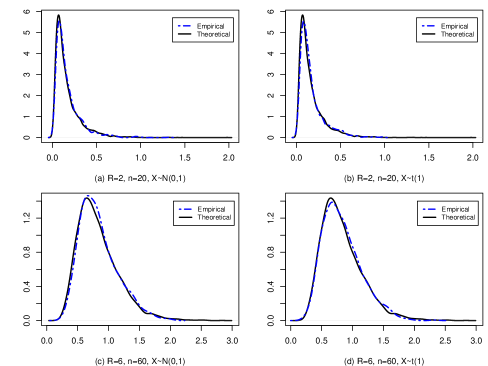
Figure 2: Comparing the empirical distribution of the MV test statistic with the asymptotic theoretical distribution under the null hypothesis. The empirical null distribution (broken) is a kernel density estimate using gaussian kernels based on 1000 values of $T_{n}$ and the asymptotic null distribution (solid) is obtained in (3.2).

The next theorem shows that under the alternative hypothesis, the MV test statistic diverges to infinity as $n\rightarrow\infty$. In other words, if $X$ and $Y$ are dependent, i.e. $MV(X|Y)>0$, the power of the MV test to reject the false null hypothesis converges to one as $n$ approaches the infinity. Thus, the MV test is a consistent test.

Theorem 3.2.

Suppose that the conditions assumed in Lemma 2.2 hold. Under the alternative hypothesis $H_{1}$, we have

$$T_{n}=n\widehat{MV}(X|Y)\overset{p}{\longrightarrow}\infty,\mbox{~{}~{}as~{}~{}}n\to\infty,$$ (3.3)

where $\overset{p}{\longrightarrow}$ denotes the convergence in probability.

Then, we study the asymptotic normality of $\widehat{MV}(X|Y)$ which helps us to find an expression of the asymptotic power function of the MV test.

Theorem 3.3.

Under the alternative hypothesis $H_{1}$, i.e. $MV(X|Y)>0$, we have

$$\sqrt{n}(\widehat{MV}(X|Y)-MV(X|Y))\overset{d}{\longrightarrow}N(0,\sigma^{2}),$$ (3.4)

where $\sigma^{2}=Var[\sum_{r=1}^{R}I_{4r}(X,Y)]$, where $I_{4r}(X,Y)$ is given in the Appendix.

Based on Theorem 3.3, we can derive the following asymptotic power function of the MV test.

$$\beta_{n}(\Delta) = P\left(T_{n}>c_{\alpha}|MV(X|Y)=\Delta>0\right)$$ (3.5)

$$= P\left(\frac{\sqrt{n}(\widehat{MV}(X|Y)-\Delta)}{\sigma}>\frac{c_{\alpha}-n\Delta}{\sqrt{n}\sigma}\Big{|}MV(X|Y)=\Delta>0\right)$$

$$\approx 1-\Phi\left(\frac{c_{\alpha}-n\Delta}{\sqrt{n}\sigma}\right),$$

where $\Phi(\cdot)$ is the cumulative distribution function of the standard normal distribution and $c_{\alpha}$ denotes the $\alpha$ upper-tailed value of the asymptotic null distribution of the MV test statistic under $H_{0}$. It can be observed that the power $\beta_{n}(\Delta)$ increases for fixed $\Delta$ and $\alpha$ as the sample size increases. This result will also be confirmed by Monte Carlo studies in Section 4.

3.3 Implementation of MV Test

In this subsection, we discuss the implementation of the MV test in practice. The appealing feature of the MV test is that Theorem 3.1 provides the explicit asymptotic null distribution of $T_{n}$ when $R$ is fixed. Note that ${\chi_{j}^{2}(R-1)}/{\pi^{2}j^{2}}$ is ignorable when $j$ is very large. We approximate the asymptotic null distribution $\sum_{j=1}^{+\infty}{\chi_{j}^{2}(R-1)}/{\pi^{2}j^{2}}$ by $\sum_{j=1}^{N}{\chi_{j}^{2}(R-1)}/{\pi^{2}j^{2}}$ for $N$ sufficiently large in practice. We display the asymptotic null distributions of $R-1$ degrees of freedom, $R=2,3,\ldots,10$, in Figure 3. The density curves show that the asymptotic null distribution for each $R$ is right-skewed like a $\chi^{2}$ distribution and approaches to a normal distribution as $R$ increases.

Figure 3: The asymptotic null distributions of the MV test statistic.

Our empirical studies show that the asymptotic null distribution performs well even when the sample size is not large. However, if the sample size is very small, the permutation test can be used to find the p-value for the MV test. The permutation test is computationally efficient when the sample size is small. For example, Szekely, Rizzo and Bakirov (2007) applied the permutation test to their distance covariance test of independence. Heller, Heller and Corfine (2013) also used the permutation samples to compute the p-value for their test of association based on ranks of distances. However, the permutation test is not computationally efficient especially when there are many pairs of random variables needed to test. In this case, it is appealing to use our MV test based on the explicit asymptotic null distribution to save computational complexity.

3.4 Asymptotic Distribution when $R$ is Diverging

The asymptotic distributions of MV test statistic have been studied before when the number of classes is fixed. Next, we will derive its asymptotic null distribution when $R$ tends to the infinity.

Theorem 3.4.

If $\sqrt{R}/\underset{1\leq r\leq R}{\min}p_{r}=o(\sqrt{n})$ and $R\to+\infty$ as $n\to\infty$, then under $H_{0}$, we have

$$\frac{T_{n}-(R-1)/6}{\sqrt{(R-1)/45}}\overset{d}{\longrightarrow}N(0,1),\mbox{~{}as~{}}n\to\infty.$$ (3.6)

If $\underset{1\leq r\leq R}{\min}p_{r}=O(n^{-\gamma})$ where $0<\gamma<1/2$, then we can derive that $R=O(n^{\kappa})$ for some $0<\kappa<1-2\gamma$. That is, we can allow the number of subgroups go to the infinity with the sample size $n$ at a relatively slow rate. This result is another distinguished merit of our test from the existing methods. Theorem 3.4 shows that the limiting null distribution of the MV test can be approximated by a normal distribution with mean $(R-1)/6$ and variance $(R-1)/45$ when $R$ is large. To connect it to the asymptotic null distribution when $R$ is fixed in Theorem 3.1, one can note that the mean and variance of $\sum_{j=1}^{+\infty}{\chi_{j}^{2}(R-1)}/{\pi^{2}j^{2}}$ are given by

$$~{}~{}~{}~{}~{}~{}~{}~{}~{}~{}E\left(\sum_{j=1}^{+\infty}\frac{\chi_{j}^{2}(R-1)}{\pi^{2}j^{2}}\right)=\frac{R-1}{6},~{}~{}Var\left(\sum_{j=1}^{+\infty}\frac{\chi_{j}^{2}(R-1)}{\pi^{2}j^{2}}\right)=\frac{R-1}{45}.$$ (3.7)

4 Numerical Studies

4.1 Monte Carlo Simulations

In this section, we assess the finite-sample performance of the MV test (MV) of independence by comparing with other existing tests: the classic Pearson’s chi-square test (CS), the distance covariance test (DC) in Szekely, Rizzo and Bakirov (2007), and the test based on ranks of distances (HHG) in Heller, Heller and Corfine (2013) in various simulation examples. Because the Pearson’s chi-square test of independence is only applicable for two discrete/categorical random variables, we discretize equally the continuous variable into a discrete one with the same number of classes as the categorical one. The permutation test with the permutated times $K=200$ is used for the DC and HHG tests since their explicit asymptotic null distributions are not available. The DC and HHG tests are applied by calling the functions dcov.test in the R package energy (Rizzo and Szekely, 2014) and hhg.test in the R package HHG (Kaufman, 2014), respectively. Note that it is meaningless to directly apply the DC test to a categorical variable. Thus, we transfer the categorical variable with $R$ classes to a vector of $R-1$ dummy binary variables and apply dcov.test to this random vector instead of the original variable. For the MV test, we consider two ways to compute the p-value: the permutation test with $K=200$ (denoted by MV1) and the asymptotic null distribution in (3.2) (denoted by MV2) for the first three examples. In Example 4, the p-value for the MV test is obtained using an approximated normal distribution based on the asymptotic results in Theorem 3.4. All numerical studies are conducted using R code.

Example 1. We randomly generate a continuous random variable $X$ from $N(0,1)$ or t(1) and independently generate a categorical random variable $Y$ from a discrete uniform distribution with $R$ classes. Then, we test the independence between two random variables when $R=2$ or $6$. The sample sizes $n$ are chosen to be 50, 75, 100, 125 and 150. We run each simulation 1000 times to compute the empirical type-I error rates at the nominal significance level $\alpha=0.1$ and summarize the results in Table 1. Most of tests perform well since the empirical type-I error rates are close to the nominal significance level. However, when $R=2$, the Pearson’s chi-square test (CS) is relatively conservative because the information of $X$ may loss substantially after discretized into a binary variable. When $X\sim t(1)$, the distance covariance test (DC) seems conservative due to extreme values.

Table 1: Empirical type-I error rates at the significance level 0.1 in Example 1.

		$X\sim N(0,1)$					$X\sim t(1)$
$R$	$n$	MV1	MV2	DC	CS	HHG	MV1	MV2	DC	CS	HHG
	50	0.091	0.091	0.080	0.055	0.086	0.091	0.093	0.079	0.061	0.089
	75	0.115	0.118	0.105	0.065	0.103	0.100	0.106	0.095	0.075	0.102
$2$	100	0.099	0.098	0.095	0.053	0.075	0.098	0.101	0.106	0.054	0.086
	125	0.116	0.123	0.113	0.078	0.111	0.096	0.098	0.092	0.076	0.097
	150	0.095	0.097	0.099	0.061	0.090	0.097	0.098	0.100	0.068	0.109
	50	0.115	0.109	0.106	0.094	0.104	0.105	0.106	0.079	0.096	0.102
	75	0.100	0.106	0.104	0.102	0.103	0.115	0.113	0.108	0.096	0.097
$6$	100	0.093	0.093	0.094	0.107	0.083	0.083	0.091	0.084	0.092	0.089
	125	0.109	0.100	0.100	0.102	0.097	0.099	0.105	0.095	0.112	0.101
	150	0.105	0.109	0.098	0.107	0.104	0.105	0.107	0.104	0.103	0.112

Example 2. We first randomly generate a categorical random variable $Y$ from $R$ classes $\{1,2,\ldots,R\}$ with the unbalanced proportions $p_{r}=P(Y=r)=2[1+(r-1)/(R-1)]/3R$, $r=1,2,\ldots,R$, where $\{p_{1},\ldots,p_{r}\}$ is an arithmetic progression with $\underset{1\leq r\leq R}{\max}p_{r}=2\underset{1\leq r\leq R}{\min}p_{r}$. For instance, when $Y$ is binary, $p_{1}=1/3$ and $p_{2}=2/3$. Given $Y_{i}=r$, the $i$th predictor $X_{i}$ is then generated by letting $X_{i}=\mu_{r}+\varepsilon_{i}$, where $r=1,2,\ldots,R$. We consider the following two choices of $R$: (1) $R=2$, $\mu=(\mu_{1},\mu_{2})=(1,2)$ and $\varepsilon\sim N(0,1)$ or $t(1)$. (2) $R=6$, $\mu=(\mu_{1},\mu_{2},\ldots,\mu_{6})=(6,3,4,1,5,2)/3$ and $\varepsilon\sim N(0,1)$ or $t(1)$. In both cases, $X$ is dependent on the categories of $Y$, so the null hypothesis is false. Table 2 shows the empirical powers of each test for different sample sizes based on 500 simulations at $\alpha=0.05$. When $X$ is normal, all tests perform well and the MV test is slightly better than others. When the data contain extreme values, the empirical powers of the DC, CS and HHG tests deteriorate quickly while the MV test reasonably well.

Table 2: Empirical powers at $\alpha=0.05$ against the sample sizes in Example 2.

		$X\sim N(0,1)$					$X\sim t(1)$
$R$	$n$	MV1	MV2	DC	CS	HHG	MV1	MV2	DC	CS	HHG
	50	0.850	0.822	0.848	0.580	0.718	0.474	0.484	0.224	0.372	0.396
	75	0.960	0.966	0.966	0.822	0.906	0.630	0.618	0.286	0.550	0.594
$2$	100	0.986	0.988	0.988	0.942	0.970	0.758	0.758	0.406	0.704	0.708
	125	1.000	1.000	1.000	0.978	0.998	0.860	0.864	0.474	0.818	0.816
	150	1.000	1.000	1.000	0.992	0.998	0.922	0.924	0.556	0.896	0.882
	50	0.746	0.742	0.708	0.376	0.348	0.348	0.254	0.168	0.218	0.190
	75	0.958	0.930	0.936	0.780	0.700	0.542	0.402	0.264	0.384	0.296
$6$	100	0.992	0.982	0.982	0.934	0.878	0.700	0.576	0.322	0.498	0.386
	125	0.998	0.998	0.998	0.976	0.944	0.830	0.714	0.382	0.596	0.524
	150	1.000	0.998	1.000	0.994	0.988	0.892	0.816	0.456	0.736	0.652

Then, we consider local power analysis of all tests under contiguous sequence of alternative hypotheses. We fix $n=100$ and consider two cases: (1) $R=2$, $\mu=(\mu_{1},\mu_{2})=c(1,2)$, $\varepsilon\sim N(0,1)$ or $t(1)$; (2) $R=6$, $\mu=(\mu_{1},\mu_{2},\ldots,\mu_{6})=c(6,3,4,1,5,2)$ and $\varepsilon\sim N(0,1)$ or $t(1)$. The values of $c$ vary from 0 to 1, which control the signal strength against alternatives. When $c=0$, $X$ and $Y$ are statistically independent and $H_{0}$ is true; otherwise, $H_{0}$ is false. We display the empirical powers of all tests against the values of $c$ in Table 3. The MV test has the excellent power performance in most settings especially when $X$ follows $t(1)$.

Table 3: Empirical powers at $\alpha=0.05$ against the signal strength in Example 2.

		$X\sim N(0,1)$					$X\sim t(1)$
$R$	c	MV1	MV2	DC	CS	HHG	MV1	MV2	DC	CS	HHG
	0.0	0.054	0.056	0.040	0.022	0.046	0.060	0.054	0.050	0.040	0.044
	0.2	0.156	0.164	0.154	0.092	0.116	0.072	0.080	0.044	0.062	0.068
$2$	0.4	0.426	0.424	0.416	0.256	0.294	0.186	0.186	0.074	0.148	0.124
	0.6	0.722	0.736	0.732	0.508	0.590	0.354	0.354	0.128	0.312	0.316
	0.8	0.924	0.922	0.932	0.792	0.852	0.592	0.586	0.230	0.516	0.514
	1.0	0.988	0.988	0.986	0.902	0.964	0.754	0.766	0.388	0.716	0.716
	0.0	0.052	0.060	0.040	0.038	0.062	0.020	0.030	0.048	0.020	0.050
	0.2	0.642	0.656	0.600	0.318	0.272	0.680	0.690	0.194	0.400	0.290
$6$	0.4	0.998	1.000	0.996	0.946	0.896	1.000	1.000	0.708	0.970	0.900
	0.6	1.000	1.000	1.000	1.000	1.000	1.000	1.000	0.966	1.000	1.000
	0.8	1.000	1.000	1.000	1.000	1.000	1.000	1.000	1.000	1.000	1.000
	1.0	1.000	1.000	1.000	1.000	1.000	1.000	1.000	1.000	1.000	1.000

Example 3. We generate $X_{1}$ and $X_{2}$ independently from a uniform discrete distribution with 3 categories $\{-1,0,1\}$, and let $Y=X_{1}+1.5|X_{2}|+\varepsilon,$ where the random error $\varepsilon\sim N(0,1)$ or $t(1)$. This simple example mimics a genetic association model where the SNPs are regressors and some continuous trait such as the body mass index is the response. Note that the SNPs are categorical with three classes. We apply the aforementioned methods to test the independence between $Y$ and $X_{1}$, $Y$ and $X_{2}$, respectively. Table 4 summarizes the empirical powers of each test based on 500 simulations at $\alpha=0.05$. The DC test performs well when the random error is normal but the performance drops quickly when the extreme values are present. The HHG test works well for testing the independence between $Y$ and $X_{1}$ but not for the pair of $Y$ and $X_{2}$. The MV test performs well in all settings. It is also observed that the MV test based on the asymptotic null distribution (MV2) performs as well as the permutation-based MV test (MV1).

Table 4: Empirical powers at $\alpha=0.05$ against the sample sizes in Example 3.

		$\varepsilon\sim N(0,1)$					$\varepsilon\sim t(1)$
$X_{i}$	$n$	MV1	MV2	DC	CS	HHG	MV1	MV2	DC	CS	HHG
	30	0.814	0.832	0.744	0.648	0.754	0.370	0.370	0.238	0.274	0.384
	60	0.992	0.994	0.976	0.952	0.962	0.668	0.682	0.394	0.554	0.656
$X_{1}$	90	1.000	1.000	0.998	0.998	0.994	0.870	0.878	0.594	0.782	0.872
	120	1.000	1.000	1.000	1.000	1.000	0.964	0.974	0.704	0.926	0.970
	150	1.000	1.000	1.000	1.000	1.000	0.988	0.986	0.800	0.966	0.988
	30	0.616	0.624	0.640	0.388	0.316	0.286	0.276	0.190	0.208	0.142
	60	0.916	0.932	0.926	0.784	0.684	0.550	0.552	0.358	0.418	0.348
$X_{2}$	90	0.990	0.992	0.992	0.958	0.910	0.728	0.744	0.498	0.636	0.512
	120	1.000	1.000	1.000	0.990	0.966	0.850	0.864	0.636	0.786	0.670
	150	1.000	1.000	1.000	1.000	0.996	0.944	0.944	0.720	0.890	0.800

Example 4. In this example, we follow Example 2 to generate data and let the number of classes $R=20$ and the sample size $n=200$. Here, the signal vector $\mu=c(\mu_{1},\mu_{2},\ldots,\mu_{20}),$ where the values of $c$ vary from 0 to 1, each $\mu_{j}$ is randomly set to be one of $(1,2,3,4)$. Note that the p-value for the MV test is computed using the approximated normal distribution with mean $(R-1)/6$ and variance $(R-1)/45$ based on Theorem 3.4 and others are based on the permutation tests. It shows that the approximated normal null distribution of the MV statistic performs well for the large-$R$ case and further supports Theorem 3.4.

Table 5: Empirical powers at $\alpha=0.05$ against the signal strength for the large-$R$ case.

	$X\sim N(0,1)$				$X\sim t(1)$
c	MV	DC	CS	HHG	MV	DC	CS	HHG
0.0	0.052	0.056	0.042	0.068	0.050	0.042	0.042	0.056
0.2	0.366	0.382	0.182	0.166	0.118	0.110	0.062	0.068
0.4	0.974	0.982	0.284	0.722	0.502	0.152	0.130	0.126
0.6	1.000	1.000	0.818	0.966	0.896	0.414	0.296	0.246
0.8	1.000	1.000	0.990	1.000	0.982	0.672	0.542	0.432
1.0	1.000	1.000	1.000	1.000	1.000	0.892	0.814	0.578

4.2 A Real-Data Application

The colon cancer gene expression data set contains 62 tissue samples, which include 40 tumor biopsies from colorectal tumors (labelled as “negative”) and 22 normal biopsies from healthy parts of the colons (labelled as “positive”). There are 2,000 genes which were selected out of more than 6,500 human genes based on the confidence in the measured expression levels. The data have been analyzed by Alon (1999) to reveal broad coherent patterns of correlated genes that suggested a high degree of organization underlying gene expression in these tissues. It is of interest to detect the significant genes associated with the tissue syndrome.

We first applied the MV test to test for dependence between genes and the tissue groups at the significance level $\alpha=0.05$. Since 2,000 hypotheses were simultaneously tested, the Bonferroni correction was used to control the familywise error rate at 0.05. Thus, we would test each individual hypothesis at the significance level $\alpha/2000=2.5\times 10^{-5}$. The asymptotic null distribution in (3.2) was used to compute the p-value for each MV test and 8 genes were identified as significance. Figure 4 displays the MV indices of all 2000 genes with the 8 significant genes.

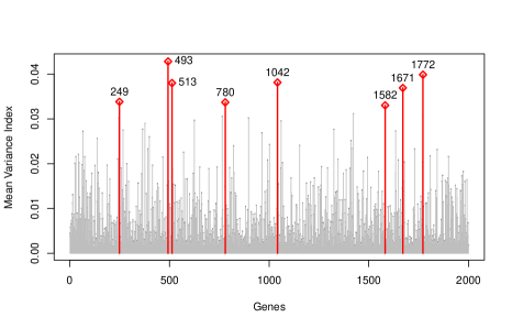
Figure 4: The MV indices of 2000 genes with the significant genes based on MV test.

Next, we applied the DC test for the gene expression data. Note that the smallest p-value obtained by the function dcov.test using $K$ permutation times is $1/(K+1)$. Thus, we chose $K=40000$ to make the DC test applicable to identify the significant genes. For the DC test, 12 genes were selected as significance. Table 6 summarizes the computation time and the significant genes. We conclude that it is very computationally efficient to conduct many simultaneous tests using the explicit asymptotic null distribution compared with the permutation test, since 2000 MV tests only took about 3 seconds.

To further check the significance of the selected genes, we randomly partitioned the data into two parts: 80% as the training data and the rest 20% as the testing samples. Then, the linear discriminant analysis was applied to the training data based on the selected significant genes. The classification accuracy (CA), i.e. the percentage of classifying test samples into the correct groups, for the testing data was computed for each test and summarized in Table 6. All models had similar predication performance. However, the MV tests had the better prediction performance based on the smaller set of significant genes. This result further demonstrated the MV test would be useful to test the significance of many genes simultaneously in high dimensional data analysis.

Table 6: Comparison among different tests in the real-data application.

Tests	Time(s)	CA	# of Genes	Indices of Significant Genes
MV	2.8	85.56%	8	$\left\{{249~{}~{}493~{}~{}513~{}~{}780~{}~{}1042~{}~{}1582~{}~{}1671~{}~{}1772}\right\}$
DC	603.4	85.01%	12	$\left\{\begin{array}[]{cccccc}245&249&267&377&493&765\\ 822&1042&1325&1423&1582&1772\end{array}\right\}$

5 Discussions

In this paper, we proposed the new distribution-free mean variance (MV) test of independence between a categorical random variable and a continuous one. We derived an explicit form of its asymptotic null distribution, $\sum_{j=1}^{+\infty}{\chi_{j}^{2}(R-1)}/{\pi^{2}j^{2}}$, where $\chi_{j}^{2}(R-1),j=1,2,\ldots$, are independent $\chi^{2}$ random variables with $R-1$ degrees of freedom. It helps us to compute the empirical p-value efficiently in practice. It is also worth noting that this result does not depend on the distributions of two random variables $X$ and $Y$. Simulations and real data analysis showed its usefulness for detecting significant variables in high dimensional data.

Two extensions of the MV test can be considered. First, the MV test is also applicable in practice to test the independence between two continuous random variables by discretizing one continuous one into a categorical one. We can discretize a random variable $X$ using its percentiles $\{\tau_{1},\ldots,\tau_{K_{n}}\}$ by defining $X_{i}^{*}=kI(\tau_{k}\leq X_{i}<\tau_{k+1}),$ where $I(\cdot)$ is an indicator function, $i=1,\ldots,n$, $k=1,\ldots,K_{n}$. If $K_{n}$ is too large, then the sample size in each class is too small and the estimation of mean variance index is inaccurate. By contrast, if $K_{n}$ is too small, then much information of the continuous variable may lose and the test power is unsatisfactory. We can choose $K_{n}=O(n^{1/3})$ as Huang and Cui (2015) suggested. In practice, we suggest to choose $K_{n}=[n/20]$, where $[a]$ means the integer part of $a$, so that the sample size in each category is around 20. How to choose an optimal $K_{n}$ and the associated power performance will be left for the future research. Second, another possible extension is to test the independent between a categorical response variable $Y$ and a random vector. Let ${\bf x}=(X_{1},\ldots,X_{J})$ be a random vector with the dimensionality $J$. We can consider an aggregating approach to defining a multivariate MV between $Y$ and ${\bf x}$ as $MV({\bf x}|Y)=J^{-1}\sum_{1\leq j\leq J}MV(X_{j}|Y)$. The theoretical properties will be left for the future research.  

6 Appendix: Proofs of Theorems

To prove Theorem 3.1, we first need to define

$$\widetilde{MV}(X|Y)=\sum_{r=1}^{R}\frac{1}{p_{r}}\int\left[\frac{1}{n}\sum_{i=1}^{n}f_{i}(x,r)\right]^{2}dF(x).$$ (A.1)

where $f_{i}(x,r)=I\{X_{i}\leq x,Y_{i}=y_{r}\}-I\{X_{i}\leq x\}p_{r}-F(x)(I\{Y_{i}=y_{r}\}-p_{r}),$ for $i=1,\ldots,n$. The following Lemma studies the difference between $\widetilde{MV}(X|Y)$ and $\widehat{MV}(X|Y)$ under the null hypothesis of independence.

Lemma A.1.

Under $H_{0}:$ $X$ and $Y$ are statistically independent, we have

$$\widehat{MV}(X|Y)-\widetilde{MV}(X|Y)=O_{p}\left(\frac{Rn^{-3/2}}{\underset{1\leq r\leq R}{\min}p_{r}}\right).$$ (A.2)

Proof of Lemma A.1: First, we let

$$\widetilde{MV}_{1}(X|Y)=\sum_{r=1}^{R}\frac{1}{p_{r}}\int\left[\frac{1}{n}\sum_{i=1}^{n}f_{i}(x,r)\right]^{2}d\hat{F}(x),$$ (A.3)

where $f_{i}(x,r)=I\{X_{i}\leq x,Y_{i}=y_{r}\}-I\{X_{i}\leq x\}p_{r}-F(x)(I\{Y_{i}=y_{r}\}-p_{r}),$ for $i=1,\ldots,n$. Next, we consider the difference between $\widehat{MV}(X|Y)$ and $\widetilde{MV}_{1}(X|Y)$. Note that

$$\widehat{MV}(X|Y) = \frac{1}{n}\sum_{r=1}^{R}\sum_{i=1}^{n}\hat{p}_{r}\left[\hat{F}_{r}(X_{i})-\hat{F}(X_{i})\right]^{2}$$

$$= \sum_{r=1}^{R}\frac{1}{\hat{p}_{r}}\int\left[\hat{F}_{r}(x)\hat{p}_{r}-\hat{F}(x)\hat{p}_{r}\right]^{2}d\hat{F}(x)$$

Thus, we have

$$\widehat{MV}(X|Y)-\widetilde{MV}_{1}(X|Y)$$

$$= \sum_{r=1}^{R}\frac{1}{\hat{p}_{r}}\int\left[\hat{F}_{r}(x)\hat{p}_{r}-\hat{F}(x)\hat{p}_{r}\right]^{2}d\hat{F}(x)-\sum_{r=1}^{R}\frac{1}{p_{r}}\int\left[\frac{1}{n}\sum_{i=1}^{n}f_{i}(x,r)\right]^{2}d\hat{F}(x)$$

$$= \sum_{r=1}^{R}\left[\frac{1}{\hat{p}_{r}}-\frac{1}{p_{r}}\right]\int\left[\hat{F}_{r}(x)\hat{p}_{r}-\hat{F}(x)\hat{p}_{r}\right]^{2}d\hat{F}(x)$$

$$+ \sum_{r=1}^{R}\frac{1}{p_{r}}\int\left\{\left[\hat{F}_{r}(x)\hat{p}_{r}-\hat{F}(x)\hat{p}_{r}\right]^{2}-\left[\frac{1}{n}\sum_{i=1}^{n}f_{i}(x,r)\right]^{2}\right\}d\hat{F}(x)$$

$$=: I_{1n}+I_{2n}$$

We deal with the first term $I_{1n}$. By the central limit theorem, we have $\hat{p}_{r}-p_{r}=O_{p}({n}^{-1/2})$. Then,

$$\frac{1}{\hat{p}_{r}}-\frac{1}{p_{r}}=\frac{\hat{p}_{r}-p_{r}}{\hat{p}_{r}p_{r}}\leq\frac{O_{p}({n}^{-1/2})}{\underset{1\leq r\leq R}{\min}p_{r}}.$$

Since

$$\hat{F}_{r}(x)\hat{p}_{r}-\hat{F}(x)\hat{p}_{r}$$

$$= \frac{1}{n}\sum_{i=1}^{n}[I\{X_{i}<x,Y_{i}=y_{r}\}-F(x)p_{r}]+F(x)p_{r}-\hat{F}(x)(\hat{p}_{r}-p_{r})-\hat{F}(x)p_{r}$$

$$= \frac{1}{n}\sum_{i=1}^{n}[I\{X_{i}<x,Y_{i}=y_{r}\}-F(x)p_{r}]-\hat{F}(x)(\hat{p}_{r}-p_{r})-[\hat{F}(x)-F(x)]p_{r},$$

by the theory of empirical process, we have that

$$\sup_{x}\left|\hat{F}_{r}(x)\hat{p}_{r}-\hat{F}(x)\hat{p}_{r}\right| \leq \sup_{x}\left|\frac{1}{n}\sum_{i=1}^{n}[I\{X_{i}<x,Y_{i}=y_{r}\}-F(x)p_{r}\right|$$

$$+ |\hat{p}_{r}-p_{r}|+\sup_{x}\left|\hat{F}(x)-F(x)\right|$$

$$= O_{p}({n}^{-1/2}),$$

where we note that $E(I\{X_{i}<x,Y_{i}=y_{r}\})=E(I\{X_{i}<x\})E(I\{Y_{i}=y_{r}\})=F(x)p_{r}$ under the null hypothesis $H_{0}$. It follows that

$$I_{1n} = \sum_{r=1}^{R}\left[\frac{1}{\hat{p}_{r}}-\frac{1}{p_{r}}\right]\int\left[\hat{F}_{r}(x)\hat{p}_{r}-\hat{F}(x)\hat{p}_{r}\right]^{2}d\hat{F}(x)$$ (A.4)

$$\leq \sum_{r=1}^{R}\left|\frac{1}{\hat{p}_{r}}-\frac{1}{p_{r}}\right|\sup_{x}\left[\hat{F}_{r}(x)\hat{p}_{r}-\hat{F}(x)\hat{p}_{r}\right]^{2}$$

$$= \frac{R}{\underset{1\leq r\leq R}{\min}p_{r}}O_{p}(n^{-3/2}).$$

Next, we deal with the second term $I_{2n}$. By the theory of empirical process, we have

$$\sup_{x}\left|\left[\hat{F}_{r}(x)\hat{p}_{r}-\hat{F}(x)\hat{p}_{r}\right]^{2}-\left[\frac{1}{n}\sum_{i=1}^{n}f_{i}(x,r)\right]^{2}\right|$$

$$= \sup_{x}\left|\hat{F}_{r}(x)\hat{p}_{r}-\hat{F}(x)\hat{p}_{r}-\frac{1}{n}\sum_{i=1}^{n}f_{i}(x,r)\right|\cdot\left|\hat{F}_{r}(x)\hat{p}_{r}-\hat{F}(x)\hat{p}_{r}+\frac{1}{n}\sum_{i=1}^{n}f_{i}(x,r)\right|$$

$$= {\sup_{x}\left|\hat{F}(x)-F(x)\right|\left|\hat{p}_{r}-p_{r}\right|}\cdot\left\{\sup_{x}\left|\hat{F}_{r}(x)\hat{p}_{r}-\hat{F}(x)\hat{p}_{r}\right|+\sup_{x}\left|\frac{1}{n}\sum_{i=1}^{n}f_{i}(x,r)\right|\right\}$$

$$= O_{p}(n^{-1/2})O_{p}(n^{-1/2})O_{p}(n^{-1/2})=O_{p}(n^{-3/2}).$$

where the second equality follows by

$$\hat{F}_{r}(x)\hat{p}_{r}-\hat{F}(x)\hat{p}_{r}-\frac{1}{n}\sum_{i=1}^{n}f_{i}(x,r)$$

$$= \left\{\frac{1}{n}\sum_{i=1}^{n}I\{X_{i}<x,Y_{i}=y_{r}\}-\hat{F}(x)\hat{p}_{r}\right\}$$

$$- \left\{\frac{1}{n}\sum_{i=1}^{n}I\{X_{i}<x,Y_{i}=y_{r}\}-\hat{F}(x)p_{r}-F(x)(\hat{p}_{r}-p_{r})\right\}$$

$$= \left[\hat{F}(x)-F(x)\right]\left(\hat{p}_{r}-p_{r}\right).$$

It follows that

$$I_{2n} = \sum_{r=1}^{R}\frac{1}{p_{r}}\int\left\{\left[\hat{F}_{r}(x)\hat{p}_{r}-\hat{F}(x)\hat{p}_{r}\right]^{2}-\left[\frac{1}{n}\sum_{i=1}^{n}f_{i}(x,r)\right]^{2}\right\}d\hat{F}(x)$$ (A.5)

$$= \frac{R}{\underset{1\leq r\leq R}{\min}p_{r}}O_{p}(n^{-3/2}).$$

Thus, (A.4) and (A.5) together imply that

$$\widehat{MV}(X|Y)-\widetilde{MV}_{1}(X|Y)=\frac{R}{\underset{1\leq r\leq R}{\min}p_{r}}O_{p}(n^{-3/2}).$$ (A.6)

To complete the proof of Lemma A.1, it is sufficient to prove that the difference between $\widetilde{MV}_{1}(X|Y)$ and $\widetilde{MV}(X|Y)$ satisfies that

$$\widetilde{MV}_{1}(X|Y)-\widetilde{MV}(X|Y) = \sum_{r=1}^{R}\frac{1}{p_{r}}\int\left[\frac{1}{n}\sum_{i=1}^{n}f_{i}(x,r)\right]^{2}d\left[\hat{F}(x)-F(x)\right]$$ (A.7)

$$= \frac{R}{\underset{1\leq r\leq R}{\min}p_{r}}O_{p}(n^{-3/2}).$$

It is enough to show

$$I_{3n}(r)=:\int\left[\frac{1}{n}\sum_{i=1}^{n}f_{i}(x,r)\right]^{2}d\left[\hat{F}(x)-F(x)\right]=O_{p}(n^{-3/2}).$$ (A.8)

Without loss of generality, we let $F(x)$ be the uniform distribution function, since we can make the transformation $X^{\prime}=F(X)$ for the continuous random variable $X$. Therefore,

$$I_{3n}(r)=\frac{1}{n}\sum_{j=1}^{n}\left[\frac{1}{n}\sum_{i=1}^{n}f_{i}(X_{j},r)\right]^{2}-\int_{0}^{1}\left[\frac{1}{n}\sum_{i=1}^{n}f_{i}(x,r)\right]^{2}dx.$$

For any $x,y\in(0,1)$, we can easily prove that

$$E[f_{i}(x,r)f_{j}(y,r)]=(x\wedge y-xy)(p_{r}-p_{r}^{2})I\{i=j\},$$

where $x\wedge y$ denotes the smaller value of $x$ and $y$.

$$E[I^{2}_{3n}(r)] = E\left\{\int_{0}^{1}\left[\frac{1}{n}\sum_{j=1}^{n}[\bar{f}(X_{j})^{2}-\bar{f}(x)^{2}]\right]dx\right\}^{2}$$

$$= E\left\{\int_{0}^{1}\int_{0}^{1}\left[\frac{1}{n}\sum_{j=1}^{n}[\bar{f}(X_{j})^{2}-\bar{f}(x)^{2}]\right]\left[\frac{1}{n}\sum_{j=1}^{n}[\bar{f}(X_{j})^{2}-\bar{f}(y)^{2}]\right]dxdy\right\}$$

$$= \int_{0}^{1}\int_{0}^{1}E\left\{[\bar{f}(X_{1})^{2}-\bar{f}(x)^{2}][\bar{f}(X_{2})^{2}-\bar{f}(y)^{2}]\right\}dxdy$$

where $\bar{f}(x)=n^{-1}\sum_{i=1}^{n}f_{i}(x,r).$

Because $E(f_{i}(x,r))=0$ under $H_{0}$, $E[f_{i}(x,r)f_{j}(x,r)f_{k}(y,r)f_{l}(y,r)]=0$ under $H_{0}$ if one of $\{i,j,k,l\}$ is different from the other three. Then, we can prove that

$$E[\bar{f}(x)^{2}\bar{f}(y)^{2}] = \frac{1}{n^{4}}\sum_{i,j}\sum_{k,l}E[f_{i}(x,r)f_{j}(x,r)f_{k}(y,r)f_{l}(y,r)]$$

$$= \frac{1}{n^{3}}E[f_{1}(x,r)^{2}f_{1}(y,r)^{2}]+\frac{n-1}{n^{3}}E[f_{1}^{2}(x,r)]E[f_{2}^{2}(y,r)]$$

$$+\frac{2(n-1)}{n^{3}}\left\{E[f_{1}(x,r)f_{1}(y,r)]\right\}^{2}$$

$$= O(n^{-3})+\frac{(p_{r}-p_{r}^{2})^{2}}{n^{2}}[xy(1-x)(1-y)+2(x\wedge y-xy)^{2}].$$

Similarly, we have

$$E[\bar{f}(X_{1})^{2}\bar{f}(y)^{2}] = \frac{1}{n^{4}}\sum_{i,j}\sum_{k,l}E[f_{i}(X_{1},r)f_{j}(X_{1},r)f_{k}(y,r)f_{l}(y,r)]$$

$$= O(n^{-3})+\frac{(p_{r}-p_{r}^{2})^{2}}{n^{2}}E[X_{1}y(1-X_{1})(1-y)+2(X_{1}\wedge y-X_{1}y)^{2}]$$

$$= O(n^{-3})+\frac{(p_{r}-p_{r}^{2})^{2}}{n^{2}}\int_{0}^{1}[xy(1-x)(1-y)+2(x\wedge y-xy)^{2}]dx.$$

$$E[\bar{f}(x)^{2}\bar{f}(X_{2})^{2}] = \frac{1}{n^{4}}\sum_{i,j}\sum_{k,l}E[f_{i}(x,r)f_{j}(x,r)f_{k}(X_{2},r)f_{l}(X_{2},r)]$$

$$= O(n^{-3})+\frac{(p_{r}-p_{r}^{2})^{2}}{n^{2}}\int_{0}^{1}[xy(1-x)(1-y)+2(x\wedge y-xy)^{2}]dy.$$

$$E[\bar{f}(X_{1})^{2}\bar{f}(X_{2})^{2}] = \frac{1}{n^{4}}\sum_{i,j}\sum_{k,l}E[f_{i}(X_{1},r)f_{j}(X_{1},r)f_{k}(X_{2},r)f_{l}(X_{2},r)]$$

$$= O(n^{-3})+\frac{(p_{r}-p_{r}^{2})^{2}}{n^{2}}\int_{0}^{1}\int_{0}^{1}[xy(1-x)(1-y)+2(x\wedge y-xy)^{2}]dxdy.$$

Therefore, we have

$$E[I^{2}_{3n}(r)] = \int_{0}^{1}\int_{0}^{1}E[\bar{f}(X_{1})^{2}\bar{f}(X_{2})^{2}]dxdy-\int_{0}^{1}\int_{0}^{1}E[\bar{f}(X_{1})^{2}\bar{f}(y)^{2}]dxdy$$ (A.9)

$$- \int_{0}^{1}\int_{0}^{1}E[\bar{f}(x)^{2}\bar{f}(X_{2})^{2}]dxdy+\int_{0}^{1}\int_{0}^{1}E[\bar{f}(x)^{2}\bar{f}(y)^{2}]dxdy$$

$$= O(n^{-3}).$$

Because $E[I_{3n}(r)]=0$ for any $r$, we have $I_{3n}(r)=O_{p}(n^{-3/2}).$ This completes the proof of Lemma A.1.

Lemma A.1 further implies that the difference between $T_{n}=n\widehat{MV}(X|Y)$ and $\widetilde{T}_{n}=n\widetilde{MV}(X|Y)$ is the order of $n^{-1/2}/\underset{1\leq r\leq R}{\min}p_{r}$ in probability. That is,

$$T_{n}-\widetilde{T}_{n}=O_{p}\left(\frac{Rn^{-1/2}}{\underset{1\leq r\leq R}{\min}p_{r}}\right),$$

This lemma paves a road to derive the asymptotic null distribution of $T_{n}$ in Theorem 3.1.

Proof of Theorem 3.1: Based on the result of Lemma A.1, it is sufficient to prove that

$$n\widetilde{MV}(X|Y) = \sum_{r=1}^{R}\frac{1}{p_{r}}\int\left[\frac{1}{\sqrt{n}}\sum_{i=1}^{n}f_{i}(x,r)\right]^{2}dF(x)$$ (A.10)

$$\overset{d}{\longrightarrow} \sum_{j=1}^{+\infty}\frac{\chi_{j}^{2}(R-1)}{\pi^{2}j^{2}}$$

Denote $b_{R}=(\sqrt{p_{1}},\sqrt{p_{2}},\cdots,\sqrt{p_{R}})^{\prime}$ and $B=(b_{1},b_{2},\cdots,b_{R})^{\prime}$, where $b_{1},b_{2},\ldots,b_{R-1}\in{\bf R}^{R}$ are $R-1$ unit and orthogonal vectors such that $B$ is an orthogonal matrix.

$${\bf g}(x) = B\left(\frac{f(x,1)}{\sqrt{p_{1}}},\frac{f(x,2)}{\sqrt{p_{2}}},\cdots,\frac{f(x,R)}{\sqrt{p_{R}}}\right)^{\prime},$$

$$\hat{\bf g}_{i}(x) = B\left(\frac{f_{i}(x,1)}{\sqrt{p_{1}}},\frac{f_{i}(x,2)}{\sqrt{p_{2}}},\cdots,\frac{f_{i}(x,R)}{\sqrt{p_{R}}}\right)^{\prime},$$

where $f(x,r)=I\{X\leq x,Y=y_{r}\}-I\{X\leq x\}p_{r}-F(x)(I\{Y=y_{r}\}-p_{r})$.

Let ${\cal G}=\{{\bf g}(x):x\in{\bf R},r=1,2,\cdots,R\}$. Since the graphical sets of $I\{X\leq x\},I\{X\leq x,Y=y_{r}\},F(x)I\{Y=y_{r}\}$ and $F(x)$ form a Vapnik-Chervonenkis($VC$) class respectively, then we have that $\cal G$ forms a polynomial $VC$ class by the Lemma in Pollard (1984), and

$$\left\{\frac{1}{\sqrt{n}}\sum_{i=1}^{n}\hat{\bf g}_{i}(x):x\in{\bf R}\right\}\rightsquigarrow\left\{Z(x)=(Z(x,1),Z(x,2),\cdots,Z(x,R))^{\prime}:x\in{\bf R}\right\}$$

by the Gaussian process convergence theorem in Pollard (1984) and Shorack and Wellner (1986), where $\rightsquigarrow$ denotes the convergence in distribution for any $x\in{\bf R}$, $\{Z(x):x\in{\bf R}\}$ is a Gaussian process with $EZ(x)=0$.

Let $C=(c_{rs})_{R\times R}$ be a $R\times R$ matrix with each element $c_{rs}$ defined by $c_{rs}=E\left\{\frac{f(x,r)}{\sqrt{p_{r}}}\frac{f(y,s)}{\sqrt{p_{s}}}\right\}$. Since $f(x,r)=[I(X\leq x)-F(x)][I(Y=y_{r})-p_{r}]$ under $H_{0}$, then

$$c_{rs}=\frac{1}{\sqrt{p_{r}p_{s}}}E\left\{f(x,r)f(y,s)\right\}$$

$$= \frac{1}{\sqrt{p_{r}p_{s}}}E\Big{\{}[I(X\leq x)-F(x)][I(Y=y_{r})-p_{r}][I(X\leq y)-F(y)][I(Y=y_{s})-p_{s}]\Big{\}}$$

$$= \frac{1}{\sqrt{p_{r}p_{s}}}E\Big{\{}[I(X\leq x)-F(x)][I(X\leq y)-F(y)]\Big{\}}E\Big{\{}[I(Y=y_{r})-p_{r}][I(Y=y_{s})-p_{s}]\Big{\}}$$

Note that $E\Big{\{}[I(X\leq x)-F(x)][I(X\leq y)-F(y)]\Big{\}}=F(x)\wedge F(y)-F(x)F(y).$ If $s=r$, $E\Big{\{}[I(Y=y_{r})-p_{r}][I(Y=y_{s})-p_{s}]\Big{\}}=E\{[I(Y=y_{r})-p_{r}]\}^{2}=p_{r}(1-p_{r})$. If $s\neq r$, $E\Big{\{}[I(Y=y_{r})-p_{r}][I(Y=y_{s})-p_{s}]\Big{\}}=-p_{r}p_{s}.$ Then

$$C=[F(x)\wedge F(y)-F(x)F(y)][I_{R}-b_{R}b_{R}^{\prime}],$$

where $I_{R}$ denotes the $R\times R$ identity matrix. Note that

$$B(I_{R}-b_{R}b_{R}^{\prime})B^{\prime}=BB^{\prime}-Bb_{R}(Bb_{R})^{\prime}=I_{R}-\mbox{diag}(0,\ldots,0,1)=\mbox{diag}(I_{R-1},0),$$

where $I_{R-1}$ denotes the $(R-1)\times(R-1)$ identity matrix. Thus, we have

$$E[Z(x,r)Z(y,s)] = E[{\bf g}(x){\bf g}(y)^{\prime}]_{r,s}=(BCB^{\prime})_{rs}$$ (A.13)

$$= [F(x)\wedge F(y)-F(x)F(y)](B(I-b_{R}b_{R}^{\prime})B^{\prime})_{rs}$$

$$= [F(x)\wedge F(y)-F(x)F(y)](\mbox{diag}(I_{R-1},0))_{rs}$$

$$= \left\{\begin{array}[]{lll}&F(x)\wedge F(y)-F(x)F(y),&\ \ s=r=1,2,\cdots,R-1,\\ &0,&\ \ \mbox{otherwise}.\end{array}\right.$$

It implies that $Z(x,r)$ and $Z(y,s)$ are independent if $s\neq r$. By applying the continuous mapping theorem, we have

$$\left\{\left\|\frac{1}{\sqrt{n}}\sum_{i=1}^{n}\hat{\bf g}_{i}(x)\right\|^{2}:x\in{\bf R}\right\}\rightsquigarrow\left\{\|Z(x)\|^{2}:x\in{\bf R}\right\}.$$ (A.14)

Therefore,

$$\sum_{r=1}^{R}\frac{1}{p_{r}}\int\left[\frac{1}{\sqrt{n}}\sum_{i=1}^{n}f_{i}(x,r)\right]^{2}dF(x)$$ (A.15)

$$= \int\left\|\frac{1}{\sqrt{n}}\sum_{i=1}^{n}\hat{\bf g}_{i}(x)\right\|^{2}dF(x)\overset{d}{\longrightarrow}\int\|Z(x)\|^{2}dF(x)$$

$$= \sum_{r=1}^{R-1}\int Z^{2}(x,r)dF(x)\overset{d}{=}\sum_{r=1}^{R-1}\sum_{j=1}^{+\infty}\frac{\chi_{rj}^{2}(1)}{\pi^{2}j^{2}}\overset{d}{=}\sum_{j=1}^{+\infty}\frac{\chi_{j}^{2}(R-1)}{\pi^{2}j^{2}},$$ (A.16)

where $\chi_{rj}^{2}(1)$’s denote the independently and identically distributed (i.i.d.) $\chi^{2}$ random variables with $1$ degrees of freedom and $\chi_{j}^{2}(R-1)$’s are i.i.d. $\chi^{2}$ random variables with $R-1$ degrees of freedom, the convergence in distribution $\overset{d}{\longrightarrow}$ follows the continuous mapping theorem, the second equality sign is based on that $Z(x,r)$ and $Z(y,s)$ are independent if $s\neq r$ and the result (A.13), the first $\overset{d}{=}$ is implied by Section 4.4 in Durbin (1973) or Section 6.3.4 in Hajek, Sidak and Sen (1999) . This completes the proof of Theorem 3.1.

Proof of Theorem 3.2: Under the conditions assumed in Lemma 2.2 hold, we have, under the alternative hypothesis $H_{1}$, $\widehat{MV}(X|Y)\overset{p}{\rightarrow}MV(X|Y)>0$, as $n\rightarrow\infty$. By Slutsky’s theorem, we have $T_{n}=n\widehat{MV}(X|Y)\overset{p}{\longrightarrow}\infty,\mbox{~{}~{}as~{}~{}}n\to\infty.$ This completes the proof of Theorem 3.2.

Proof of Theorem 3.3: For any $1\leq r\leq R$, we have $\int(\hat{F}_{r}-\hat{F})^{2}d\hat{F}(x)=\int(F_{r}-F)^{2}dF(x)+o_{p}(1)$ and

$$\int[(\hat{F}_{r}-\hat{F})^{2}-(F_{r}-F)^{2}]d\hat{F}(x)$$

$$= \int[\hat{F}_{r}-\hat{F}-(F_{r}-F)][\hat{F}_{r}-\hat{F}+(F_{r}-F)]d\hat{F}(x)$$

$$= 2\int(F_{r}-F)[\hat{F}_{r}-\hat{F}-(F_{r}-F)]dF(x)+o_{p}(n^{-1/2})$$

$$= \frac{2}{\hat{p}_{r}}\int(F_{r}-F)[\hat{F}_{r}\hat{p}_{r}-F_{r}\hat{p}_{r}]dF(x)-2\int(F_{r}-F)(\hat{F}-F)]dF(x)+o_{p}(n^{-1/2})$$

$$= \frac{2}{p_{r}}\int(F_{r}-F)[\hat{F}_{r}\hat{p}_{r}-F_{r}p_{r}-F_{r}(\hat{p}_{r}-p_{r})]dF(x)$$

$$-2\int(F_{r}-F)(\hat{F}-F)]dF(x)+o_{p}(n^{-1/2})$$

$$= -\frac{2}{p_{r}}\int(F_{r}-F)F_{r}dF(x)(\hat{p}_{r}-p_{r})+\frac{2}{p_{r}}\int(F_{r}-F)[\hat{F}_{r}\hat{p}_{r}-F_{r}p_{r}]dF(x)$$

$$-2\int(F_{r}-F)(\hat{F}-F)]dF(x)+o_{p}(n^{-1/2}).$$

Thus, we have

$$\widehat{MV}(X|Y)-MV(X|Y)=\sum_{r=1}^{R}\left\{\hat{p}_{r}\int(\hat{F}_{r}-\hat{F})^{2}d\hat{F}(x)-p_{r}\int(F_{r}-F)^{2}dF(x)\right\}$$

$$= \sum_{r=1}^{R}\left\{(\hat{p}_{r}-p_{r})\int(\hat{F}_{r}-\hat{F})^{2}d\hat{F}(x)+p_{r}\int[(\hat{F}_{r}-\hat{F})^{2}-(F_{r}-F)^{2}]d\hat{F}(x)\right.$$

$$\left.+p_{r}\int(F_{r}-F)^{2}d(\hat{F}(x)-F(x))\right\}$$

$$= \sum_{r=1}^{R}\left\{(\hat{p}_{r}-p_{r})\int(F_{r}-F)^{2}dF(x)+2p_{r}\int(F_{r}-F)[\hat{F}_{r}-\hat{F}-(F_{r}-F)]dF(x)\right.$$

$$+\left.p_{r}\int(F_{r}-F)^{2}d(\hat{F}(x)-F(x))\right\}+o_{p}(n^{-1/2})$$

$$= \sum_{r=1}^{R}\left\{\int(F^{2}-F_{r}^{2})dF(x)(\hat{p}_{r}-p_{r})+2\int(F_{r}-F)[\hat{F}_{r}\hat{p}_{r}-F_{r}p_{r}]dF(x)\right.$$

$$\left.-2p_{r}\int(F_{r}-F)(\hat{F}-F)]dF(x)+p_{r}\int(F_{r}-F)^{2}d(\hat{F}(x)-F(x))\right\}+o_{p}(n^{-1/2})$$

$$=: \frac{1}{n}\sum_{i=1}^{n}\sum_{r=1}^{R}I_{4r}(X_{i},Y_{i})+o_{p}(n^{-1/2}),$$

where

$$I_{4r}(X,Y) =: \int(F^{2}-F_{r}^{2})dF(x)(I\{Y=y_{r}\}-p_{r})$$

$$+ 2\int(F_{r}-F)(I\{X<x,Y=y_{r}\}-F_{r}p_{r})dF(x)$$

$$- 2p_{r}\int(F_{r}-F)(I\{X<x\}-F(x))dF(x)$$

$$+ p_{r}[(F_{r}(X)-F(X))^{2}-\int(F_{r}(x)-F(x))^{2}dF(x)],$$

and $EI_{4r}(X_{i},Y_{i})=0$. Then by the Limit Central Theorem, we have

$$\sqrt{n}[\widehat{MV}(X|Y)-MV(X|Y)]=\frac{1}{\sqrt{n}}\sum_{i=1}^{n}\sum_{r=1}^{R}I_{4r}(X_{i},Y_{i})+o_{p}(1)\overset{d}{\longrightarrow}N(0,\sigma^{2}).$$

This completes the proof of Theorem 3.3.  

Proof of Theorem 3.4: First, we can prove the following three results.

$$(i).\ \ E[f_{i}(x,r)f_{i}(y,s)] = (x\bigwedge y-xy)(p_{r}\delta_{rs}-p_{r}p_{s}),$$

$$(ii).\ E[f_{i}^{2}(x,r)f_{i}^{2}(y,s)] \leq C[p_{r}\delta_{rs}+p_{r}p_{s}(p_{r}+p_{s})],$$

for all $1\leq i\leq n,1\leq r,s\leq R$, where $C$ is a positive constant and $\delta_{rs}=1$ if $r=s$, $\delta_{rs}=0$ otherwise.

(iii).

$$\sum_{r,s,t,q=1}^{R}\frac{1}{p_{r}p_{s}p_{t}p_{q}}(p_{r}\delta_{rs}-p_{r}p_{s})(p_{r}\delta_{rt}-p_{r}p_{t})(p_{t}\delta_{tq}-p_{t}p_{q})(p_{s}\delta_{sq}-p_{s}p_{q})=O(R).$$

Then, with loss of generality, we assume that $X\sim Unif(0,1)$, then $F(x)=x$ for $0\leq x\leq 1$. According to Lemma A.1, we have

$$T_{n}-\widetilde{T}_{n}=O\left(\frac{Rn^{-1/2}}{\underset{1\leq r\leq R}{\min}p_{r}}\right),$$

where $\widetilde{T}_{n}=n\widetilde{MV}(X|Y)$. Then, under the condition $\sqrt{R}/\underset{1\leq r\leq R}{\min}p_{r}=o(\sqrt{n})$, we have that $T_{n}-\widetilde{T}_{n}=o(\sqrt{R}).$ Thus, it suffices to prove that

$$\frac{\widetilde{T}_{n}-(R-1)/6}{\sqrt{(R-1)/45}}\overset{d}{\longrightarrow}N(0,1).$$

Write

$$\widetilde{T}_{n}=\frac{1}{n}\sum_{r=1}^{R}\frac{1}{p_{r}}\int\left[\sum_{i=1}^{n}f_{i}(x,r)\right]^{2}dx=:J_{1n}+J_{2n},$$

where

$$J_{1n}=\frac{1}{n}\sum_{i=1}^{n}\sum_{r=1}^{R}\frac{1}{p_{r}}\int f_{i}^{2}(x,r)dx,\mbox{~{}~{}and~{}~{}}J_{2n}=\frac{1}{n}\sum_{i\neq j}^{n}\sum_{r=1}^{R}\frac{1}{p_{r}}\int f_{i}(x,r)f_{j}(x,r)dx.$$

Note that $f_{i}(x,r)=(I(X_{i}\leq x)-x)(I(Y_{i}=y_{r})-p_{r})$, then

$$E(J_{1n}) = \sum_{r=1}^{R}\frac{1}{p_{r}}E\left[\int(I(X_{1}\leq x)-x)^{2}(I(Y_{1}=y_{r})-p_{r})^{2}dx\right]$$

$$= \sum_{r=1}^{R}\frac{1}{p_{r}}E\left[(I(Y_{1}=y_{r})-p_{r})^{2}\int(I(X_{1}\leq x)-2xI(X_{1}\leq x)+x^{2})dx\right]$$

$$= \sum_{r=1}^{R}\frac{1}{p_{r}}E\left[(I(Y_{1}=y_{r})-p_{r})^{2}\times\frac{1}{6}\right]$$

$$= \sum_{r=1}^{R}\frac{1}{p_{r}}p_{r}(1-p_{r})/6=(R-1)/6,$$

and

$$Var(J_{1n}) = \frac{1}{n}Var\left[\sum_{r=1}^{R}\frac{1}{p_{r}}\int f_{1}^{2}(x,r)dx\right]\leq\frac{1}{n}E\left[\sum_{r=1}^{R}\frac{1}{p_{r}}\int f_{1}^{2}(x,r)dx\right]^{2}$$

$$= \frac{1}{n}\sum_{r,s}^{R}\frac{1}{p_{r}p_{s}}\int\int E[f_{1}^{2}(x,r)f_{1}^{2}(y,s)]dxdy$$

$$\leq \frac{C}{n}\sum_{r,s}^{R}\frac{1}{p_{r}p_{s}}(p_{r}\delta_{rs}+p_{r}p_{s}(p_{r}+p_{s}))$$

$$= \frac{C}{n}\left(\frac{R}{\min p_{r}}+R\right)=o(1).$$

Next, we then only show that

$$\frac{J_{2n}}{\sqrt{(R-1)/45}}\overset{d}{\longrightarrow}N(0,1).$$

Note that $E(J_{2n})=0$ and

$$Var(J_{2n}) = E(J_{2n}^{2})=\frac{1}{n^{2}}\sum_{i\neq j,k\neq l}^{n}\sum_{r,s}^{R}\frac{1}{p_{r}p_{s}}\int\int E[f_{i}(x,r)f_{j}(x,r)f_{k}(y,s)f_{l}(y,s)]dxdy$$

$$= \frac{2n(n-1)}{n^{2}}\sum_{r,s}^{R}\frac{1}{p_{r}p_{s}}\int\int\{E[f_{1}(x,r)f_{2}(y,s)]\}^{2}dxdy$$

$$= (1-\frac{1}{n})\frac{R-1}{45}.$$

Let ${\cal F}_{i}=\sigma\{(X_{1},Y_{1}),\cdots,(X_{i},Y_{i})\}$. We also see that

$$\frac{J_{2n}}{\sqrt{(R-1)/45}}=\frac{\sum_{i=2}^{n}\big{[}\frac{2}{n}\sum_{j=1}^{i-1}\sum_{r=1}^{R}\frac{1}{p_{r}}\int f_{i}(x,r)f_{j}(x,r)dx\big{]}}{\sqrt{(R-1)/45}}=:\sum_{i=2}^{n}Z_{ni}$$

is the summation of a Martingale difference sequence with $E(Z_{ni})=0$ and $Var[\sum_{i=2}^{n}Z_{ni}]=1-\frac{1}{n}\to 1.$ We need to prove $\sum_{i=2}^{n}E(Z_{ni}^{2}|{\cal F}_{i-1})\overset{p}{\rightarrow}1$. Since $E[\sum_{i=2}^{n}E(Z_{ni}^{2}|{\cal F}_{i-1})]\to 1$ and

$$E(Z_{ni}^{2}|{\cal F}_{i-1}) = \frac{45}{R-1}(\frac{2}{n})^{2}\sum_{j,k}^{i-1}\sum_{r,s}^{R}\frac{1}{p_{r}p_{s}}\int\int E[f_{i}(x,r)f_{i}(y,s)]f_{j}(x,r)f_{k}(y,s)dxdy$$

$$= \frac{45}{R-1}(\frac{2}{n})^{2}\sum_{j,k}^{i-1}\sum_{r,s}^{R}\frac{p_{r}\delta_{rs}-p_{r}p_{s}}{p_{r}p_{s}}\int\int(x\bigwedge y-xy)f_{j}(x,r)f_{k}(y,s)dxdy.$$

Thus, we have

$$\sum_{i=2}^{n}E(Z_{ni}^{2}|{\cal F}_{i-1}) = \frac{45}{R-1}(\frac{2}{n})^{2}\sum_{j=1}^{n-1}(n-j)\sum_{r,s}^{R}\frac{1}{p_{r}p_{s}}\int\int E[f_{i}(x,r)f_{i}(y,s)]f_{j}(x,r)f_{j}(y,s)dxdy$$

$$+ \frac{45}{R-1}(\frac{2}{n})^{2}\sum_{j<k\leq n}(n-k)\sum_{r,s}^{R}\frac{1}{p_{r}p_{s}}\int\int E[f_{i}(x,r)f_{i}(y,s)]f_{j}(x,r)f_{k}(y,s)dxdy$$

$$=: J_{3n}+J_{4n}.$$

Since $E(J_{3n})\to 1$, $E(J_{4n})=0$ and $Var(J_{3n})\leq\frac{CR^{2}\sum_{j=1}^{n-1}(n-j)^{2}}{(R-1)^{2}n^{4}}=O(1/n)$, then $J_{3n}\overset{p}{\rightarrow}1$.

$$Var(J_{4n}) = (\frac{45}{R-1})^{2}(\frac{2}{n})^{4}\sum_{j<k,l<m}(n-k)(n-m)$$

$$E\Big{(}\sum_{r,s}^{R}\frac{1}{p_{r}p_{s}}\int\int E[f_{i}(x,r)f_{i}(y,s)]f_{j}(x,r)f_{k}(y,s)dxdy$$

$$\sum_{r,s}^{R}\frac{1}{p_{r}p_{s}}\int\int E[f_{i}(x,r)f_{i}(y,s)]f_{l}(x,r)f_{m}(y,s)dxdy\Big{)}$$

$$= (\frac{45}{R-1})^{2}(\frac{2}{n})^{4}\sum_{j<k,l<m}(n-k)(n-m)O(R)=O(1/R).$$

Therefore, $J_{4n}\overset{p}{\rightarrow}0$. On the other hand,

$$\sum_{i=2}^{n}E(Z_{ni}^{4}) \leq \frac{C}{nR^{2}}E\Big{(}\sum_{r=1}^{R}\frac{1}{p_{r}}\int f_{1}(x,r)f_{2}(x,r)dx\Big{)}^{4}$$

$$\leq \frac{C}{nR^{2}}\Big{(}\sum_{r,s}^{R}\frac{1}{p_{r}p_{s}}\int\int E[f_{1}^{2}(x,r)f^{2}(y,s)]dxdy\Big{)}^{2}$$

$$\leq \frac{C}{nR^{2}}\Big{(}\sum_{r,s}^{R}\frac{1}{p_{r}p_{s}}[p_{r}\delta_{rs}+p_{r}p_{s}(p_{r}+p_{s})]\Big{)}^{2}=O\left(\frac{1}{n(\underset{1\leq r\leq R}{\min}{p_{r}})^{2}}\right)=o(1/R)$$

By the central limit theorem of the Martingale difference, we have

$$\frac{\tilde{T}_{n}-(R-1)/6}{\sqrt{(R-1)/45}}\overset{d}{\longrightarrow}N(0,1),~{}~{}\mbox{as}~{}n\rightarrow\infty.$$

This completes the proof of Theorem 3.4.

References

12007AgrestiAgresti (2007)Agresti:2007 Agresti, A. (2007). An introduction to categorical data analysis, 2nd ed. New York: John Wiley & Sons. 21999AlonAlon (1999)Alon:1999 Alon, U., Barkai, N., Notterman, D. A., Gish, K., Ybarra, S., Mack, D., and Levine, A. J. (1999). Broad patterns of gene expression revealed by clustering analysis of tumor and normal colon tissues probed by oligonucleotide arrays. Proc. Natl. Acad. Sci. 96 6745-6750. 31952Anderson and DarlingAnderson and Darling (1952)AD:1952 Anderson, T. W., and Darling, D. A. (1952). Asymptotic theory of certain ‘goodness-of-fit’ criteria based on stochastic processes. Ann. Math. Statist. 23 193-212. 42014Bergsma and DassiosBergsma and Dassios (2014)Bergsma:Dassios:2014 Bergsma, W. and Dassios, A. (2014). A consistent test of independence based on a sign covariance related to Kendall’s tau. Bernoulli 20 1006–1028. 52015Cui, Li and ZhongCui, Li and Zhong (2015)Cui:Li:Zhong:2014 Cui, H., Li, R. and Zhong, W. (2015). Model-free feature screening for ultrahigh dimensional discriminant analysis. J. Amer. Statist. Assoc. 110 630–641. 61973DurbinDurbin (1973)Durbin:1973 Durbin, J. (1973). Distribution theory for tests based on the sample distribution function. SIAM, Philadelphia, PA. 71999Hajek, Sidak and SenHajek, Sidak and Sen (1999)Hajek:1999 Hajek, J., Sidak, Z. and Sen, P. (1999). Theory of rank tests, 2nd ed. Academic Press, San Diego, CA. 82013Heller, Heller and CorfineHeller, Heller and Corfine (2013)HHG:2013 Heller, R., Heller, Y. and Corfine, M. (2013). A consistent multivariate test of association based on ranks of distances. Biometrika 100 503–510. 91948HoeffdingHoeffding (1948)Hoeffding:1948 Hoeffding, W. (1948). A non-parametric test of independence. Ann. Math. Statist. 19 546–557. 102015Huang and CuiHuang and Cui (2015)Huang:Cui:2015 Huang, R. and Cui, H. (2015). Consistency of chi-squared test with varying number of classes. J. Sys. Sci. Complex. 28 1–12. 112014KaufmanKaufman (2014)Kaufman:2014 Kaufman, S. and based in part on an earlier implementation by Ruth Heller and Yair Heller. (2014). HHG: Heller-Heller-Gorfine Tests of Independence. R package version 1.4. http://CRAN.R-project.org/package=HHG 121984PollardPollard (1984)Pollard:1984 Pollard, D. (1984). Convergence of stochastic processes. Springer-Verlag, New York Inc. 131976PettittPettitt (1976)Pettitt:1976 Pettitt, A. N. (1976). A two-sample Anderson-Darling rank statistic. Biometrika. 63 161-168. 142014Rizzo and SzekelyRizzo and Szekely (2014)Rizzo:Szekely:2014 Rizzo, M. L. and Székely, G. J. (2014). energy: E-statistics (energy statistics). R package version 1.6.1. http://CRAN.R-project.org/package=energy 151975RosenblattRosenblatt (1975)Rosenblatt:1975 Rosenblatt, M. (1975). A quadratic measure of deviation of two-dimensional density estimates and a test of independence. Ann. Statist. 3 1–14. 161986Shorack and WellnerShorack and Wellner (1986)Shorack:Wellner:1986 Shorack, G. and Wellner J. (1986). Empirical Processes with Applications in Statistics. Wiley, New York, Inc. 172007Szekely, Rizzo and BakirovSzekely, Rizzo and Bakirov (2007)Szekely:Rizzo:Bakirov:2007 Székely, G. J., Rizzo, M. L. and Bakirov, N. K. (2007), Measuring and testing dependence by correlation of distances. Ann. Statist. 35 2769–2794. 182009Szekely and RizzoSzekely and Rizzo (2009)Szekely:Rizzo:2009 Székely, G. J. and Rizzo, M. L. (2009). Brownian distance covariance. Ann. Appl. Statist. 3 1236–1265.