Strong Coordination of Signals and Actions over Noisy Channels with two-sided State Information

Abstract

We consider a network of two nodes separated by a noisy channel with two-sided state information, in which the input and output signals have to be coordinated with the source and its reconstruction. In the case of non-causal encoding and decoding, we propose a joint source-channel coding scheme and develop inner and outer bounds for the strong coordination region. While the inner and outer bounds do not match in general, we provide a complete characterization of the strong coordination region in three particular cases: i) when the channel is perfect; ii) when the decoder is lossless; and iii) when the random variables of the channel are independent from the random variables of the source. Through the study of these special cases, we prove that the separation principle does not hold for joint source-channel strong coordination. Finally, in the absence of state information, we show that polar codes achieve the best known inner bound for the strong coordination region, which therefore offers a constructive alternative to random binning and coding proofs.

I Introduction

While communication networks have traditionally been designed as “bit pipes” meant to reliably convey information, the anticipated explosion of device-to-device communications, e.g., as part of the Internet of Things, is creating new challenges. In fact, more than communication by itself, what is crucial for the next generation of networks is to ensure the cooperation and coordination of the constituent devices, viewed as autonomous decision makers. In the present work, coordination is meant in the broad sense of enforcing a joint behavior of the devices through communication. More specifically, we shall quantify this joint behavior in terms of how well we can approximate a target joint distribution between the actions and signals of the devices. Our main objective in the present work is to characterize the amount of communication that is required to achieve coordination for several networks.

A general information-theoretic framework to study coordination in networks was put forward in [3], related to earlier work on “Shannon’s reverse coding theorem” [4] and the compression of probability distribution sources and mixed quantum states [5, 6, 7]. This framework also relates to the game-theoretic perspective on coordination [8] with applications, for instance, power control [9]. Recent extensions of the framework have included the possibility of coordination through interactive communication [10, 11]. Two information-theoretic metrics have been proposed to measure the level of coordination: empirical coordination, which requires the joint histogram of the devices’ actions to approach a target distribution, and strong coordination, which requires the joint distribution of sequences of actions to converge to an i.i.d. target distribution, e.g., in variational distance [3, 12]. Empirical coordination captures an “average behavior” over multiple repeated actions of the devices; in contrast, strong coordination captures the behavior of sequences. A byproduct of strong coordination is that it enforces some level of “security,” in the sense of guaranteeing that sequence of actions will be unpredictable to an outside observer beyond what is known about the target joint distribution of sequences.

Strong coordination in networks was first studied over error free links [3] and later extended to noisy communication links [11]. In the latter setting, the signals that are transmitted and received over the physical channel become a part of what can be observed, and one can therefore coordinate the actions of the devices with their communication signals [13, 14]. From a security standpoint, this joint coordination of actions and signals allows one to control the information about the devices’ actions that may be inferred from the observations of the communication signals. This “secure coordination” was investigated for error-free links in [15].

In the present paper, we address the problem of strong coordination in a two-node network comprised of an information source and a noisy channel, in which both nodes have access to a common source of randomness. This scenario presents two conflicting goals: the encoder needs to convey a message to the decoder to coordinate the actions, while simultaneously coordinating the signals coding the message. As in [16, 17, 18] we introduce a random state capturing the effect of the environment, to model actions and channels that change with external factors, and we consider a general setting in which state information and side information about the source may or may not be available at the decoder. We derive an inner and an outer bound for the strong coordination region by developing a joint source-channel scheme in which an auxiliary codebook allows us to satisfy both goals. Since the two bounds do not match, the optimality of our general achievability scheme remains an open question. We, however, succeeded to characterize the strong coordination region exactly in some special cases: i) when the channel is noiseless; ii) when the decoder is lossless; and iii) when the random variables of the channel are independent from the random variables of the source. In all these cases, the set of achievable target distributions is the same as for empirical coordination [17], but we show that a positive rate of common randomness is required for strong coordination. We conclude the paper by considering the design of an explicit coordination scheme in this setting. Coding schemes for coordination based on polar codes have already been designed in [19, 20, 21, 22]. Inspired by the binning technique using polar codes in [23], we propose an explicit polar coding scheme that achieves the inner bound for the coordination capacity region in [1] by extending our coding scheme in [2] to strong coordination. We use a chaining construction as in [24, 25] to ensure proper alignment of the polarized sets.

The remainder of the paper is organized as follows. Section II introduces the notation and some preliminary results. Section III describes a simple model in which there is no state and no side information and derives an inner and an outer bound for the strong coordination region. The information-theoretic modeling of coordination problems relevant to this work is best illustrated in this simplified scenario. Section IV extends the inner and outer bounds to the general case of a noisy channel with state and side information at the decoder. In particular, the inner bound is proved by proposing a random binning scheme and a random coding scheme that have the same statistics. Section V characterizes the strong coordination region for three special cases and shows that the separation principle does not hold for strong coordination. Section VI presents an explicit polar coding scheme for the simpler setting where there is no state and no side information. Finally, Section VII presents some conclusions and open problems.

II Preliminaries

We define the integer interval $\llbracket a,b\rrbracket$ as the set of integers between $a$ and $b$. Given a random vector $X^{n}:=$ $(X_{1},\ldots,X_{n})$, we note $X^{i}$ the first $i$ components of $X^{n}$, $X_{\sim i}$ the vector $(X_{j})_{j\neq i}$, $j\in\llbracket 1,n\rrbracket$, where the component $X_{i}$ has been removed and $X[A]$ the vector $(X_{j})_{j\in A}$, $A\subseteq\llbracket 1,n\rrbracket$. The total variation between two probability mass functions $P$ and $Q$ on $\mathcal{A}$ is given by

$$\mathbb{V}(P,Q):=\frac{1}{2}\sum_{a\in\mathcal{A}}\lvert P(a)-Q(a)\rvert.$$

The Kullback-Leibler divergence between two discrete distributions $P$ and $Q$ is

$$\mathbb{D}(P\Arrowvert Q):=\sum_{a}P(a)\log{\frac{P(a)}{Q(a)}}.$$

We use the notation $f(\varepsilon)$ to denote a function which tends to zero as $\varepsilon$ does, and the notation $\delta(n)$ to denote a function which tends to zero exponentially as $n$ goes to infinity.

We now state some useful results. First, we recall well-known properties of the variational distance and Kullback-Leibler divergence.

Lemma 1 ([26, Lemma 1])

Given a pair of random variables $(A,B)$ with joint distribution $P_{AB}$, marginals $P_{A}$ and $P_{B}$ and $\lvert\mathcal{A}\rvert\geq 4$, we have

$$\frac{1}{2\log 2}{\mathbb{V}(P_{AB},P_{A}P_{B})}^{2}\leq I(A;B)\leq\mathbb{V}(P_{AB},P_{A}P_{B})\log{\frac{\lvert\mathcal{A}\rvert}{\mathbb{V}(P_{AB},P_{A}P_{B})}}.$$

Lemma 2 ([27, Lemma 16])

For any two joint distributions $P_{AB}$ and $\widehat{P}_{AB}$, the total variation distance between them can only be reduced when attention is restricted to $P_{A}$ and $\widehat{P}_{A}$. That is,

$$\operatorname{\mathbb{V}}(P_{A},\widehat{P}_{A})\leq\operatorname{\mathbb{V}}(P_{AB},\widehat{P}_{AB}).$$

Lemma 3 ([27, Lemma 17])

When two random variables are passed through the same channel, the total variation between the resulting input-output joint distributions is the same as the total variation between the input distributions. Specifically,

$$\operatorname{\mathbb{V}}(P_{A},\widehat{P}_{A})=\operatorname{\mathbb{V}}(P_{A}P_{B|A},\widehat{P}_{A}P_{B|A}).$$

Lemma 4

When two random variables are passed through the same channel, the Kullback-Leibler divergence between the resulting input-output joint distributions is the same as the Kullback-Leibler divergence between the input distributions. Specifically,

$$\operatorname{\mathbb{D}}\left(P_{A}\Arrowvert\widehat{P}_{A}\right)=\operatorname{\mathbb{D}}\left(P_{A}P_{B|A}\Arrowvert\widehat{P}_{A}P_{B|A}\right).$$

Lemma 5 ([28, Lemma 4])

If $\operatorname{\mathbb{V}}\left(P_{Y^{n}}P_{X^{n}|Y^{n}},P^{\prime}_{Y^{n}}P^{\prime}_{X^{n}|Y^{n}}\right)=\varepsilon$ then there exists $\mathbf{y}\in\mathcal{Y}^{n}$ such that

$$\operatorname{\mathbb{V}}\left(P_{X^{n}|Y^{n}=\mathbf{y}},P^{\prime}_{X^{n}|Y^{n}=\mathbf{y}}\right)=2\varepsilon.$$

The proofs of the following results are in Appendix A. The following lemma is in the same spirit as [12, Lemma VI.3]. We state a slightly different version which is more convenient for our proofs.

Lemma 6

Let $P_{A^{n}}$ such that $\operatorname{\mathbb{V}}\left(P_{A^{n}},\bar{P}_{A}^{\otimes n}\right)\leq\varepsilon,$ then we have

$$\sum_{t=1}^{n}I(A_{t};A_{\sim t})\leq nf(\varepsilon).$$

In particular, if $P_{AB}$ is such that $\operatorname{\mathbb{V}}\left(P_{AB},\bar{P}_{A}\bar{P}_{B}\right)\leq\varepsilon$, then $I(A;B)\leq f(\varepsilon)$.

Lemma 7

Let $P_{A^{n}B^{n}}$ such that $\operatorname{\mathbb{V}}\left(P_{A^{n}B^{n}},\bar{P}_{AB}^{\otimes n}\right)\leq\varepsilon$. Then we have

$$\sum_{t=1}^{n}I(A_{t};A^{t-1}B_{\sim t}|B_{t})\leq nf(\varepsilon).$$ (1)

Let the variable $T$ serve as a random time index, for any random variable $C$ we have

$$H(C|B^{n})\geq nI(A_{T};CB_{\sim T}T|B_{T})-nI(A_{T}B_{T};T)-nf(\varepsilon).$$ (2)

III Inner and outer bounds for the strong coordination region

III-A System model

Figure 1: Coordination of signals and actions for a two-node network with a noisy channel with non-causal encoder and decoder.

Before we study the general model with a state in detail, it is helpful to consider a simpler model depicted in Figure 1 to understand the nature of the problem. Two agents, the encoder and the decoder, wish to coordinate their behaviors: the stochastic actions of the agents should follow a known and fixed joint distribution.

We suppose that the encoder and the decoder have access to a shared source of uniform randomness $C\in\llbracket 1,2^{nR_{0}}\rrbracket$. Let $U^{n}\in\mathcal{U}^{n}$ be an i.i.d. source with distribution $\bar{P}_{U}$. The encoder observes the sequence $U^{n}\in\mathcal{U}^{n}$ and selects a signal $X^{n}=f_{n}(U^{n},C)$, $f_{n}:\mathcal{U}^{n}\times\llbracket 1,2^{nR_{0}}\rrbracket\rightarrow\mathcal{X}^{n}$. The signal $X^{n}$ is transmitted over a discrete memoryless channel parametrized by the conditional distribution $\bar{P}_{Y|X}$. Upon observing $Y^{n}$ and common randomness $C$, the decoder selects an action $V^{n}=g_{n}(Y^{n},C)$, where $g_{n}:\mathcal{Y}^{n}\times\llbracket 1,2^{nR_{0}}\rrbracket\rightarrow\mathcal{V}^{n}$ is a stochastic map. For block length $n$, the pair $(f_{n},g_{n})$ constitutes a code.

We recall the definitions of achievability and of the coordination region for empirical and strong coordination [3, 27].

Definition 1

A distribution $\bar{P}_{UXYV}$ is achievable for empirical coordination if for all $\varepsilon>0$ there exists a sequence $(f_{n},g_{n})$ of encoders-decoders such that

$$\mathbb{P}\left\{\operatorname{\mathbb{V}}\left(T_{U^{n}X^{n}Y^{n}V^{n}},\bar{P}_{UXYV}\right)>\varepsilon\right\}<\varepsilon$$

where $T_{U^{n}X^{n}Y^{n}V^{n}}$ is the joint histogram of the actions induced by the code. The empirical coordination region $\mathcal{R}_{e}$ is the closure of the set of achievable distributions $\bar{P}_{UXYV}$.

Definition 2

A pair $(\bar{P}_{UXYV},R_{0})$ is achievable for strong coordination if there exists a sequence $(f_{n},g_{n})$ of encoders-decoders with rate of common randomness $R_{0}$, such that

$$\lim_{n\to\infty}\operatorname{\mathbb{V}}\left(P_{U^{n}X^{n}Y^{n}V^{n}},\bar{P}_{UXYV}^{\otimes n}\right)=0$$

where $P_{U^{n}X^{n}Y^{n}V^{n}}$ is the joint distribution induced by the code. The strong coordination region $\mathcal{R}$ is the closure of the set of achievable pairs $(\bar{P}_{UXYV},R_{0})$.

Our first result is an inner and outer bound for the strong coordination region $\mathcal{R}$ [1].

Theorem 1

Let $\bar{P}_{U}$ and $\bar{P}_{Y|X}$ be the given source and channel parameters, then $\mathcal{R}^{\prime}_{\text{in}}\subseteq\mathcal{R}\subseteq\mathcal{R}^{\prime}_{\text{out}}$ where:

$$\mathcal{R}^{\prime}_{\text{in}} :=\begin{Bmatrix}[c|l]&\bar{P}_{UXYV}=\bar{P}_{U}\bar{P}_{X|U}\bar{P}_{Y|X}\bar{P}_{V|UXY}\\ &\exists\mbox{ }W\mbox{ taking values in $\mathcal{W}$}\\ (\bar{P}_{UXYV},R_{0})&\bar{P}_{UXYWV}=\bar{P}_{U}\bar{P}_{W|U}\bar{P}_{X|UW}\bar{P}_{Y|X}\bar{P}_{V|WY}\\ &I(W;U)\leq I(W;Y)\\ &R_{0}\geq I(W;UXV|Y)\\ \end{Bmatrix}$$ (3)

$$\quad\mathcal{R}^{\prime}_{\text{out}} :=\begin{Bmatrix}[c|l]&\bar{P}_{UXYV}=\bar{P}_{U}\bar{P}_{X|U}\bar{P}_{Y|X}\bar{P}_{V|UXY}\\ &\exists\mbox{ }W\mbox{ taking values in $\mathcal{W}$}\\ (\bar{P}_{UXYV},R_{0})&\bar{P}_{UXYWV}=\bar{P}_{U}\bar{P}_{W|U}\bar{P}_{X|UW}\bar{P}_{Y|X}\bar{P}_{V|WY}\\ &I(W;U)\leq I(X;Y)\\ &R_{0}\geq I(W;UXV|Y)\\ &\lvert\mathcal{W}\rvert\leq\lvert\mathcal{U}\times\mathcal{X}\times\mathcal{Y}\times{\mathcal{V}}\rvert+4\\ \end{Bmatrix}.$$ (4)

Remark 1

Observe that the decomposition of the joint distributions $\bar{P}_{UXYV}$ and $\bar{P}_{UWXYV}$ is equivalently characterized in terms of Markov chains:

$$Y-X-U,\quad\quad\begin{cases}Y-X-(U,W)\\ V-(Y,W)-(X,U)\end{cases}.$$ (5)

Remark 2

The empirical coordination region for the setting of Figure 1 was investigated in [13], in which the authors derived an inner and outer bound. Note that the information constraint $I(W;U)\leq$ $I(W;Y)$ and the decomposition of the joint probability distribution $\bar{P}_{U}\bar{P}_{W|U}\bar{P}_{X|UW}\bar{P}_{Y|X}\bar{P}_{V|WY}$ are the same for empirical coordination [13, Theorem 1]. The main difference is that strong coordination requires a positive rate of common randomness $R_{0}>I(W;UXV|Y)$.

III-B Proof of Theorem 1: inner bound

We postpone the achievability proof because it is a corollary of the inner bound in the general setting of Theorem 2 proven in Section IV-A. A stand-alone proof can be found in the conference version of the present paper [1].

Remark 3

With the same random binning techniques, [11] characterizes an inner bound for the strong coordination region in the slightly different scenario in which only $U^{n}$ and $V^{n}$ need to be coordinated. Given the source and channel parameters $\bar{P}_{U}$ and $\bar{P}_{Y|X}$ respectively, the inner bound in [11] is:

$$\mathcal{R}_{\text{Hadd,in}}:=\begin{Bmatrix}[c|l]&\bar{P}_{UXYV}=\bar{P}_{U}\bar{P}_{X|U}\bar{P}_{Y|X}\bar{P}_{V|UXY}\\ &\exists\mbox{ }W\mbox{ taking values in $\mathcal{W}$}\\ (\bar{P}_{UV},R_{0})&\bar{P}_{UXYWV}=\bar{P}_{U}\bar{P}_{WX|U}\bar{P}_{Y|X}\bar{P}_{V|WY}\\ &I(W;U)\leq I(W;Y)\\ &R_{0}\geq I(W;UV)-I(W;Y)\\ \end{Bmatrix}.$$ (6)

Note that the joint distribution and the information constraints are the same as in (3) but in (3) the rate of common randomness is larger since

$$I(W;UXV|Y)=I(W;UXYV)-I(W;Y)\geq I(W;UV)-I(W;Y).$$

The difference in common randomness rate $I(W;XY|UV)$ stems from the requirement in [11], which coordinates $U^{n}$ and $V^{n}$ but not necessarly $(U^{n},X^{n},Y^{n},V^{n})$.

III-C Proof of Theorem 1: outer bound

Consider a code $(f_{n},g_{n})$ that induces a distribution $P_{U^{n}X^{n}Y^{n}V^{n}}$ that is $\varepsilon$-close in total variational distance to the i.i.d. distribution $\bar{P}_{UXYV}^{\otimes n}$. Let the random variable $T$ be uniformly distributed over the set $\llbracket 1,n\rrbracket$ and independent of sequence $(U^{n},X^{n},Y^{n},V^{n},C)$. The variable $T$ will serve as a random time index. The variable $U_{T}$ is independent of $T$ because $U^{n}$ is an i.i.d. source sequence [3].

III-C1 Bound on $R_{0}$

We apply Lemma 7 to $A^{n}:=U^{n}X^{n}V^{n}$, $B^{n}:=Y^{n}$ and $C$ and, using (2), we have

$$nR_{0}\geq H(C)\geq H(C|B^{n})$$

$$\overset{(a)}{\geq}nI(A_{T};CB_{\sim T}T|B_{T})-nI(A_{T}B_{T};T)-nf(\varepsilon)$$ (7)

$$\overset{(b)}{\geq}nI(A_{T};CB_{\sim T}T|B_{T})-2nf(\varepsilon)=nI(U_{T}X_{T}V_{T};CY_{\sim T}T|Y_{T})-2nf(\varepsilon)$$

where $(a)$ follows from Lemma 7 and $(b)$ comes from [12, Lemma VI.3].

III-C2 Information constraint

We have

$$0\overset{(a)}{\leq}I(X^{n};Y^{n})-I(C,U^{n};Y^{n})$$

$$\leq I(X^{n};Y^{n})-I(U^{n};Y^{n}|C)$$

$$=H(Y^{n})-H(Y^{n}|X^{n})+H(U^{n}|Y^{n}C)-H(U^{n}|C)$$

$$\overset{(b)}{\leq}\sum_{t=1}^{n}H(Y_{t})\!-\!\sum_{t=1}^{n}H(Y_{t}|X_{t})+\!\sum_{t=1}^{n}H(U_{t}|U^{t-1}Y_{t}Y_{\sim t}C)\!-\!\sum_{t=1}^{n}H(U_{t})$$

$$\overset{(c)}{\leq}\sum_{t=1}^{n}\left(H(Y_{t})-H(Y_{t}|X_{t})+H(U_{t}|Y_{\sim t}C)-H(U_{t})\right)$$

$$\overset{(d)}{\leq}nH(Y_{T})-nH(Y_{T}|X_{T}T)+nH(U_{T}|Y_{\sim T}CT)-nH(U_{T}|T)$$

$$\overset{(e)}{=}nH(Y_{T})-nH(Y_{T}|X_{T})+nH(U_{T}|Y_{\sim T}CT)-nH(U_{T})$$

$$=nI(X_{T};Y_{T})-nI(U_{T};Y_{\sim T},C,T)$$

where $(a)$ comes from the Markov chain $Y^{n}-X^{n}-(C,U^{n})$ and $(b)$ comes from the chain rule for the conditional entropy and the fact that $U^{n}$ is an i.i.d. source independent of $C$. The inequalities $(c)$ and $(d)$ come from the fact that conditioning does not increase entropy and $(e)$ from the memoryless nature of the channel $\bar{P}_{Y|X}$ and the i.i.d. nature of the source $\bar{P}_{U}$.

III-C3 Identification of the auxiliary random variable

We identify the auxiliary random variables $W_{t}$ with $(C,Y_{\sim t})$ for each $t\in\llbracket 1,n\rrbracket$ and $W$ with $(W_{T},T)=(C,Y_{\sim T},T)$. For each $t\in\llbracket 1,n\rrbracket$ the following two Markov chains hold:

$$Y_{t}-X_{t}-(C,Y_{\sim t},U_{t})\quad \Longleftrightarrow\quad Y_{t}-X_{t}-(W_{t},U_{t})$$ (8)

$$V_{t}-(C,Y_{\sim t},Y_{t})-(U_{t},X_{t})\quad \Longleftrightarrow\quad V_{t}-(W_{t},Y_{t})-(U_{t},X_{t})$$ (9)

where (8) comes from the fact that the channel is memoryless and (9) from the fact that the decoder is non-causal and for each $t\in\llbracket 1,n\rrbracket$ the decoder generates $V_{t}$ from $Y^{n}$ and common randomness $C$. Then, we have

$$Y_{T}-X_{T}-(C,Y_{\sim T},U_{T},T)\quad \Longleftrightarrow\quad Y_{T}-X_{T}-(W_{T},U_{T},T)$$ (10)

$$V_{T}-(C,Y_{\sim T},Y_{T},T)-(U_{T},X_{T})\quad \Longleftrightarrow\quad V_{T}-(W_{T},Y_{T},T)-(U_{T},X_{T})$$ (11)

where (10) holds because

$$\mathbb{P}\{Y_{T}=y|X_{T}=x,Y_{\sim T}=\tilde{\mathbf{y}},U_{T}=u,T=t,C\}=\mathbb{P}\{Y_{T}=y|X_{T}=x\}$$

since the channel is memoryless. Then by (9), (11) holds because

$$I(V_{T};U_{T}X_{T}|CY^{n}T)=\sum_{i=1}^{n}\frac{1}{n}I(V_{t};U_{t}X_{t}|CY^{n}T=t)=0.$$

Since $W=W_{t}$ when $T=t$, we also have $(U,X)-(W,Y)-V$ and $Y-X-(U,W)$. The cardinality bound is proved in Appendix G.

IV Inner and outer bounds for the strong coordination region with state and side information

Figure 2: Coordination of signals and actions for a two-node network with a noisy channel with state and side information at the decoder.

In this section we consider the model depicted in Figure 2. It is a generalization of the simpler setting of Figure 1, where the noisy channel depends on a state $S^{n}$, and the decoder has access to non-causal side information $Z^{n}$. The encoder selects a signal $X^{n}=f_{n}(U^{n},C)$, with $f_{n}:\mathcal{U}^{n}\times\llbracket 1,2^{nR_{0}}\rrbracket\rightarrow\mathcal{X}^{n}$ and transmits it over the discrete memoryless channel $\bar{P}_{Y|XS}$ where $S$ represents the state. The decoder then selects an action $V^{n}=g_{n}(Y^{n},Z^{n},C)$, where $g_{n}:\mathcal{Y}^{n}\times\mathcal{Z}^{n}\times\llbracket 1,2^{nR_{0}}\rrbracket\rightarrow\mathcal{V}^{n}$ is a stochastic map and $Z^{n}$ represents the side information available at the decoder.

Remark 4

Note that the channel state information and side information at the decoder are represented explicitly by the random variables $S^{n}$ and $Z^{n}$ respectively, but the model is quite general and includes scenarios where partial or perfect channel state information is available at the encoder as well, since the variables $U^{n}$ and $S^{n}$ are possibly correlated.

We recall the notions of achievability and of the coordination region for empirical and strong coordination [3, 27] in this setting.

Definition 3

A distribution $\bar{P}_{USZXYV}$ is achievable for empirical coordination if for all $\varepsilon>0$ there exists a sequence $(f_{n},g_{n})$ of encoders-decoders such that

$$\mathbb{P}\left\{\operatorname{\mathbb{V}}\left(T_{U^{n}S^{n}Z^{n}X^{n}Y^{n}V^{n}},\bar{P}_{USZXYV}\right)>\varepsilon\right\}<\varepsilon$$

where $T_{U^{n}S^{n}Z^{n}X^{n}Y^{n}V^{n}}$ is the joint histogram of the actions induced by the code. The empirical coordination region $\mathcal{R}_{e}$ is the closure of the set of achievable distributions $\bar{P}_{USZXYV}$.
A pair $(\bar{P}_{USZXYV},R_{0})$ is achievable for strong coordination if there exists a sequence $(f_{n},g_{n})$ of encoders-decoders with rate of common randomness $R_{0}$, such that

$$\lim_{n\to\infty}\operatorname{\mathbb{V}}\left(P_{U^{n}S^{n}Z^{n}X^{n}Y^{n}V^{n}},\bar{P}_{USZXYV}^{\otimes n}\right)=0$$

where $P_{U^{n}S^{n}Z^{n}X^{n}Y^{n}V^{n}}$ is the joint distribution induced by the code. The strong coordination region $\mathcal{R}$ is the closure of the set of achievable pairs $(\bar{P}_{USZXYV},R_{0})$.

In the case of non-causal encoder and decoder, the problem of characterizing the strong coordination region for the system model in Figure 2 is still open, but we establish the following inner and outer bounds.

Theorem 2

Let $\bar{P}_{USZ}$ and $\bar{P}_{Y|XS}$ be the given source and channel parameters, then $\mathcal{R}_{\text{in}}\subseteq\mathcal{R}\subseteq\mathcal{R}_{\text{out}}$ where:

$$\mathcal{R}_{\text{in}} :=\begin{Bmatrix}[c|l]&\bar{P}_{USZXYV}=\bar{P}_{USZ}\bar{P}_{X|U}\bar{P}_{Y|XS}\bar{P}_{V|UXYSZ}\\ &\exists\mbox{ }W\mbox{ taking values in $\mathcal{W}$}\\ (\bar{P}_{USZXYV},R_{0})&\bar{P}_{USZWXYV}=\bar{P}_{USZ}\bar{P}_{W|U}\bar{P}_{X|UW}\bar{P}_{Y|XS}\bar{P}_{V|WYZ}\\ &I(W;U)\leq I(W;YZ)\\ &R_{0}\geq I(W;USXV|YZ)\\ \end{Bmatrix}$$ (12)

$$\mathcal{R}_{\text{out}} :=\begin{Bmatrix}[c|l]&\bar{P}_{USZXYV}=\bar{P}_{USZ}\bar{P}_{X|U}\bar{P}_{Y|XS}\bar{P}_{V|UXYSZ}\\ &\exists\mbox{ }W\mbox{ taking values in $\mathcal{W}$}\\ (\bar{P}_{USZXYV},R_{0})&\bar{P}_{USZWXYV}=\bar{P}_{USZ}\bar{P}_{W|U}\bar{P}_{X|UW}\bar{P}_{Y|XS}\bar{P}_{V|WYZ}\\ &I(W;U)\leq\min\{I(XUS;YZ),I(XS;Y)+I(U;Z)\}\\ &R_{0}\geq I(W;USXV|YZ)\\ &\lvert\mathcal{W}\rvert\leq\lvert\mathcal{U}\times\mathcal{S}\times\mathcal{Z}\times\mathcal{X}\times\mathcal{Y}\times{\mathcal{V}}\rvert+5\\ \end{Bmatrix}$$ (13)

Remark 5

As in Theorem 1, even if inner and outer bound do not match, they only differ on the upper bound on $I(W;U)$. Note that we cannot compare $I(XUS;YZ)$ and $I(XS;Y)+I(U;Z)$ (for more details, see the discussion in Appendix C). Hence, in $\mathcal{R}_{\text{out}}$ the upper bound on the mutual information $I(W;U)$ is the minimum of the two.

Remark 6

Observe that the decomposition of the joint distributions $\bar{P}_{USZXYV}$ and $\bar{P}_{USZWXYV}$ is equivalently characterized in terms of Markov chains:

$$\begin{cases}Z-(U,S)-(X,Y)\\ Y-(X,S)-U\end{cases},\quad\begin{cases}Z-(U,S)-(X,Y,W)\\ Y-(X,S)-(U,W)\\ V-(Y,Z,W)-(X,S,U)\end{cases}.$$ (14)

IV-A Proof of Theorem 2: inner bound

The achievability proof uses the same techniques as in [11] inspired by [28]. The key idea of the proof is to define a random binning and a random coding scheme, each of which induces a joint distribution, and to prove that the two schemes have the same statistics.

Before defining the coding schemes, we state the results that we will use to prove the inner bound.

The following lemma is a consequence of the Slepian-Wolf Theorem .

Lemma 8 (Source coding with side information at the decoder [29, Theorem 10.1] )

Given a discrete memoryless source $(A^{n},B^{n})$, where $B^{n}$ is side information available at the decoder, we define a stochastic encoder $\psi_{n}:\mathcal{A}^{n}\to\llbracket 1,2^{nR}\rrbracket$, where $C:=\varphi_{n}(A^{n})$ is a binning of $A^{n}$. If $R>H(A|B)$, the decoder recovers $A^{n}$ from $C$ and $B^{n}$ with arbitrarily small error probability.

Lemma 9 (Channel randomness extraction [30, Lemma 3.1] and [28, Theorem 1])

Given a discrete memoryless source $(A^{n},B^{n})$, we define a stochastic encoder $\varphi_{n}:\mathcal{B}^{n}\to\llbracket 1,J_{n}\rrbracket$, where $K:=\varphi_{n}(B^{n})$ is a binning of $B^{n}$ with $J_{n}$ values chosen independently and uniformly at random. if $R<H(B|A)$, then we have

$$\lim_{n\to\infty}\mathbb{E}_{\varphi_{n}}\left[\mathbb{V}\left(P_{A^{n}K}^{\varphi},Q_{K}P_{A^{n}}\right)\right]=0,$$

where $\mathbb{E}_{\varphi_{n}}$ denotes the average over the random binnings and $Q_{K}$ is the uniform distribution on $\llbracket 1,J_{n}\rrbracket$.

Although Lemma 9 ensures the convergence in total variational distance and is therefore enough to prove strong coordination, it does not bring any insight on the speed of convergence. For this reason, throughout the proof we will use the following lemma instead. We omit the proof as it follows directly from the discussion in [31, Section III.A].

Lemma 10 (Channel randomness extraction for discrete memoryless sources and channels)

Let $A^{n}$ with distribution $P_{A^{n}}$ be a discrete memoryless source and $P_{B^{n}|A^{n}}$ a discrete memoryless channel. Then for every $\varepsilon>0$, there exists a sequence of $(J_{n},n)$ codes $\varphi_{n}:\mathcal{B}^{n}\to\llbracket 1,J_{n}\rrbracket$ and a constant $\alpha>0$ such that for $K:=\varphi_{n}(B^{n})$ we have

$$\liminf_{n\to\infty}\frac{\log{J_{n}}}{n}\leq(1-\varepsilon)H(B|A)\quad\mbox{and}\quad\mathbb{D}\left(P_{A^{n}K}\Arrowvert P_{A^{n}}Q_{K}\right)\leq 2^{-\alpha n}.$$ (15)

IV-A1 Random binning scheme

Assume that the sequences $U^{n}$, $S^{n}$, $Z^{n}$, $X^{n}$, $W^{n}$, $Y^{n}$ and $V^{n}$ are jointly i.i.d. with distribution

$$\bar{P}_{U^{n}S^{n}Z^{n}}\bar{P}_{W^{n}|U^{n}}\bar{P}_{X^{n}|W^{n}U^{n}}\bar{P}_{Y^{n}|X^{n}S^{n}}\bar{P}_{V^{n}|W^{n}Y^{n}Z^{n}}.$$

We consider two uniform random binnings for $W^{n}$:

• first binning $C=\varphi_{1}(W^{n})$, where $\varphi_{1}:\mathcal{W}^{n}\to\llbracket 1,2^{nR_{0}}\rrbracket$ is an encoder which maps each sequence of $\mathcal{W}^{n}$ uniformly and independently to the set $\llbracket 1,2^{nR_{0}}\rrbracket$;

• second binning $F=\varphi_{2}(W^{n})$, where $\varphi_{2}:\mathcal{W}^{n}\to\llbracket 1,2^{n\tilde{R}}\rrbracket$ is an encoder.

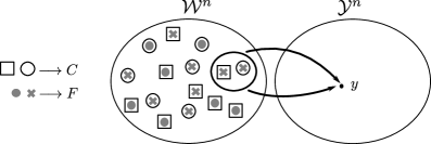
Figure 3: The square and the circle represent the possible outputs $C$ of the first binning and the dot and the cross the outputs $F$ of the second binning. Given $\mathbf{y}$ and the realizations of $C$ and $F$, it is possible to recover $\mathbf{w}$.

Note that if $\tilde{R}+R_{0}>H(W|YZ)$, by Lemma 8, it is possible to recover $W^{n}$ from $Y^{n}$, $Z^{n}$ and $(C,F)$ with high probability using a Slepian-Wolf decoder via the conditional distribution $P^{\text{SW}}_{\widehat{W}^{n}|CFY^{n}Z^{n}}$. This defines a joint distribution:

$$\bar{P}_{U^{n}S^{n}Z^{n}W^{n}\widehat{W}^{n}X^{n}Y^{n}CFV^{n}}=\bar{P}_{U^{n}S^{n}Z^{n}}\bar{P}_{W^{n}|U^{n}}\bar{P}_{X^{n}|W^{n}U^{n}}\bar{P}_{C|W^{n}}\bar{P}_{F|W^{n}}\bar{P}_{Y^{n}|X^{n}S^{n}}\bar{P}_{V^{n}|W^{n}Y^{n}Z^{n}}P^{\text{SW}}_{\widehat{W}^{n}|CFY^{n}Z^{n}}.$$

In particular, $\bar{P}_{W^{n}|CFU^{n}}$ is well defined.

IV-A2 Random coding scheme

In this section we follow the approach in [28, Section IV.E]. Suppose that in the setting of Figure 2, encoder and decoder have access not only to common randomness $C$ but also to extra randomness $F$, where $C$ is generated uniformly at random in $\llbracket 1,2^{nR_{0}}\rrbracket$ with distribution $Q_{C}$ and $F$ is generated uniformly at random in $\llbracket 1,2^{n\tilde{R}}\rrbracket$ with distribution $Q_{F}$ independently of $C$. Then, the encoder generates $W^{n}$ according to $\bar{P}_{W^{n}|CFU^{n}}$ defined above and $X^{n}$ according to $\bar{P}_{X^{n}|U^{n}W^{n}}$. The encoder sends $X^{n}$ through the channel. The decoder obtains $(Y^{n},Z^{n})$ and $(C,F)$ and reconstructs $W^{n}$ via the conditional distribution $P^{\text{SW}}_{\widehat{W}^{n}|CFY^{n}Z^{n}}$. The decoder then generates $V^{n}$ letter by letter according to the distribution $P_{V^{n}|\widehat{W}^{n}Y^{n}Z^{n}}$ (more precisely $\bar{P}_{V^{n}|W^{n}Y^{n}Z^{n}}(\widehat{\mathbf{u}}|\widehat{\mathbf{w}},\mathbf{y},\mathbf{z})$, where $\widehat{\mathbf{w}}$ is the output of the Slepian-Wolf decoder). This defines a joint distribution:

$$P_{U^{n}S^{n}Z^{n}W^{n}\widehat{W}^{n}X^{n}Y^{n}CFV^{n}}=Q_{C}Q_{F}P_{U^{n}S^{n}Z^{n}}\bar{P}_{W^{n}|CFU^{n}}\bar{P}_{X^{n}|W^{n}U^{n}}\bar{P}_{Y^{n}|X^{n}S^{n}}P^{\text{SW}}_{\widehat{W}^{n}|CFY^{n}Z^{n}}P_{V^{n}|\widehat{W}^{n}Y^{n}Z^{n}}.$$

We want to show that the distribution $\bar{P}$ is achievable for strong coordination:

$$\lim_{n\to\infty}\operatorname{\mathbb{V}}(\bar{P}_{U^{n}S^{n}Z^{n}X^{n}W^{n}\widehat{W}^{n}Y^{n}V^{n}},P_{U^{n}S^{n}Z^{n}X^{n}W^{n}\widehat{W}^{n}Y^{n}V^{n}})=0.$$ (16)

We prove that the random coding scheme possesses all the properties of the initial source coding scheme stated in Section IV-A1. Note that

$$\mathbb{D}(\bar{P}_{U^{n}S^{n}Z^{n}W^{n}\widehat{W}^{n}X^{n}Y^{n}CF}\Arrowvert P_{U^{n}S^{n}Z^{n}W^{n}\widehat{W}^{n}X^{n}Y^{n}CF})$$

$$=\mathbb{D}(\bar{P}_{U^{n}S^{n}Z^{n}}\bar{P}_{W^{n}|U^{n}}\bar{P}_{X^{n}|W^{n}U^{n}}\bar{P}_{C|W^{n}}\bar{P}_{F|W^{n}}\bar{P}_{Y^{n}|X^{n}S^{n}}P^{\text{SW}}_{\widehat{W}^{n}|CFY^{n}Z^{n}}$$

$$\phantom{=\mathbb{D}|}\Arrowvert Q_{C}Q_{F}P_{U^{n}S^{n}Z^{n}}\bar{P}_{W^{n}|CFU^{n}}\bar{P}_{X^{n}|W^{n}U^{n}}\bar{P}_{Y^{n}|X^{n}S^{n}}P^{\text{SW}}_{\widehat{W}^{n}|CFY^{n}Z^{n}})$$ (17)

$${\overset{{(a)}}{=}}\mathbb{D}(\bar{P}_{U^{n}S^{n}Z^{n}}\bar{P}_{W^{n}|U^{n}}\bar{P}_{C|W^{n}}\bar{P}_{F|W^{n}}\Arrowvert Q_{C}Q_{F}P_{U^{n}S^{n}Z^{n}}\bar{P}_{W^{n}|CFU^{n}})$$

$${\overset{{(b)}}{=}}\mathbb{D}(\bar{P}_{U^{n}S^{n}Z^{n}CF}\Arrowvert P_{U^{n}S^{n}Z^{n}}Q_{C}Q_{F})$$

where $(a)$ comes from Lemma 4. Note that $(b)$ follows from Lemma 4 as well, since $W^{n}$ is generated according to $\bar{P}_{W^{n}|CFU^{n}}$ and because of the Markov chain $W-U-ZS$, $W^{n}$ is conditionally independent of $(Z^{n},S^{n})$ given $U^{n}$. Then if $R_{0}+\widetilde{R}<H(W|USZ)=H(W|U)$, we apply Lemma 10 where $B^{n}=W^{n}$, $K=(C,F)$, and claim that there exists a fixed binning $\varphi^{\prime}:=(\varphi^{\prime}_{1},\varphi^{\prime}_{2})$ such that, if we denote with $\bar{P}^{\varphi^{\prime}}$ and $P^{\varphi^{\prime}}$ the distributions $\bar{P}$ and $P$ with respect to the choice of a binning $\varphi^{\prime}$, we have

$$\mathbb{D}\left(\bar{P}_{U^{n}S^{n}Z^{n}CF}^{\varphi^{\prime}}\Arrowvert P_{U^{n}S^{n}Z^{n}}Q_{C}Q_{F}\right)=\delta(n),$$

which by (17) implies

$$\mathbb{D}\left(\bar{P}^{\varphi^{\prime}}_{U^{n}S^{n}Z^{n}W^{n}\widehat{W}^{n}X^{n}Y^{n}CF}\Arrowvert P^{\varphi^{\prime}}_{U^{n}S^{n}Z^{n}W^{n}\widehat{W}^{n}X^{n}Y^{n}CF}\right)=\delta(n).$$

Then, by Lemma 1 we have

$$\mathbb{V}\left(\bar{P}^{\varphi^{\prime}}_{U^{n}S^{n}Z^{n}W^{n}\widehat{W}^{n}X^{n}Y^{n}CF},P^{\varphi^{\prime}}_{U^{n}S^{n}Z^{n}W^{n}\widehat{W}^{n}X^{n}Y^{n}CF}\right)=\delta(n).$$ (18)

From now on, we will omit ${\varphi^{\prime}}$ to simplify the notation.

Now we would like to show that we have strong coordination for $V^{n}$ as well, but in the second coding scheme $V^{n}$ is generated using the output of the Slepian-Wolf decoder $\widehat{W}^{n}$ and not $W^{n}$ as in the first scheme. Because of Lemma 8, the inequality $\widetilde{R}+R_{0}>H(W|YZ)$ implies that $\widehat{W}^{n}$ is equal to $W^{n}$ with high probability and we will use this fact to show that the distributions are close in total variational distance.

First, we recall the definition of coupling and the basic coupling inequality for two random variables [32].

Definition 4

A coupling of two probability distributions $P_{A}$ and $P_{A^{\prime}}$ on the same measurable space $\mathcal{A}$ is any probability distribution $\widehat{P}_{AA^{\prime}}$ on the product measurable space $\mathcal{A}\times\mathcal{A}$ whose marginals are $P_{A}$ and $P_{A^{\prime}}$.

Proposition 1 ([32, I.2.6])

Given two random variables $A$, $A^{\prime}$ with probability distributions $P_{A}$, $P_{A^{\prime}}$, any coupling $\widehat{P}_{AA^{\prime}}$ of $P_{A}$, $P_{A^{\prime}}$ satisfies

$$\operatorname{\mathbb{V}}(P_{A},P_{A^{\prime}})\leq 2\mathbb{P}_{\widehat{P}_{AA^{\prime}}}\{A\neq A^{\prime}\}$$

Then, we apply Proposition 1 to

$$\begin{matrix}[ll]A=U^{n}S^{n}Z^{n}W^{n}X^{n}Y^{n}CF&A^{\prime}=U^{n}S^{n}Z^{n}\widehat{W}^{n}X^{n}Y^{n}CF\\ P_{A}=\bar{P}_{U^{n}S^{n}Z^{n}W^{n}X^{n}Y^{n}CF}&P_{A^{\prime}}=\bar{P}_{U^{n}S^{n}Z^{n}\widehat{W}^{n}X^{n}Y^{n}CF}\\ \end{matrix}$$

$$\mathcal{A}=\mathcal{U}\times\mathcal{S}\times\mathcal{Z}\times\mathcal{W}\times\mathcal{X}\times\mathcal{Y}\times\llbracket 1,2^{nR_{0}}\rrbracket\times\llbracket 1,2^{n\tilde{R}}\rrbracket.$$

Since $\widehat{W}^{n}$ is equal to $W^{n}$ with high probability by Lemma 8, and the probability of error goes to zero exponentially in the Slepian-Wolf Theorem [29, Theorem 10.1], we find that for the random binning scheme

$$\operatorname{\mathbb{V}}(\bar{P}_{U^{n}S^{n}Z^{n}W^{n}X^{n}Y^{n}CF},\bar{P}_{U^{n}S^{n}Z^{n}\widehat{W}^{n}X^{n}Y^{n}CF})=\delta(n).$$

This implies that:

$$\operatorname{\mathbb{V}}(\bar{P}_{U^{n}S^{n}Z^{n}W^{n}\widehat{W}^{n}X^{n}Y^{n}CF},\bar{P}_{U^{n}S^{n}Z^{n}W^{n}X^{n}Y^{n}CF}\mathds{1}_{\widehat{W}^{n}|W^{n}})=\delta(n).$$ (19)

Similarly, we apply Proposition 1 again to the random coding scheme and we have

$$\operatorname{\mathbb{V}}(P_{U^{n}S^{n}Z^{n}W^{n}\widehat{W}^{n}X^{n}Y^{n}CF},P_{U^{n}S^{n}Z^{n}W^{n}X^{n}Y^{n}CF}\mathds{1}_{\widehat{W}^{n}|W^{n}})=\delta(n).$$ (20)

Then using the triangle inequality, we find that

$$\operatorname{\mathbb{V}}(\bar{P}_{U^{n}S^{n}Z^{n}W^{n}\widehat{W}^{n}X^{n}Y^{n}CFV^{n}},P_{U^{n}S^{n}Z^{n}W^{n}\widehat{W}^{n}X^{n}Y^{n}CFV^{n}})$$

$$=\operatorname{\mathbb{V}}(\bar{P}_{U^{n}S^{n}Z^{n}W^{n}\widehat{W}^{n}X^{n}Y^{n}CF}\bar{P}_{V^{n}|W^{n}Y^{n}Z^{n}},P_{U^{n}S^{n}Z^{n}W^{n}\widehat{W}^{n}X^{n}Y^{n}CF}P_{V^{n}|\widehat{W}^{n}Y^{n}Z^{n}})$$ (21)

$$\leq\operatorname{\mathbb{V}}(\bar{P}_{U^{n}S^{n}Z^{n}W^{n}\widehat{W}^{n}X^{n}Y^{n}CF}\bar{P}_{V^{n}|W^{n}Y^{n}Z^{n}},\bar{P}_{U^{n}S^{n}Z^{n}W^{n}X^{n}Y^{n}CF}\mathds{1}_{\widehat{W}^{n}|W^{n}}\bar{P}_{V^{n}|W^{n}Y^{n}Z^{n}})$$

$$\quad+\operatorname{\mathbb{V}}(\bar{P}_{U^{n}S^{n}Z^{n}W^{n}X^{n}Y^{n}CF}\mathds{1}_{\widehat{W}^{n}|W^{n}}\bar{P}_{V^{n}|W^{n}Y^{n}Z^{n}},P_{U^{n}S^{n}Z^{n}W^{n}X^{n}Y^{n}CF}\mathds{1}_{\widehat{W}^{n}|W^{n}}P_{V^{n}|\widehat{W}^{n}Y^{n}Z^{n}})$$

$$\quad+\operatorname{\mathbb{V}}(P_{U^{n}S^{n}Z^{n}W^{n}X^{n}Y^{n}CF}\mathds{1}_{\widehat{W}^{n}|W^{n}}P_{V^{n}|W^{n}Y^{n}Z^{n}},P_{U^{n}S^{n}Z^{n}W^{n}\widehat{W}^{n}X^{n}Y^{n}CF}P_{V^{n}|\widehat{W}^{n}Y^{n}Z^{n}}).$$

The first and the third term go to zero exponentially by applying Lemma 3 to (19) and (20) respectively. Now observe that

$$\mathds{1}_{\widehat{W}^{n}|W^{n}}\bar{P}_{V^{n}|W^{n}Y^{n}Z^{n}}\!\!=\mathds{1}_{\widehat{W}^{n}|W^{n}}P_{V^{n}|\widehat{W}^{n}Y^{n}Z^{n}}$$

by definition of $P_{V^{n}|\widehat{W}^{n}Y^{n}Z^{n}}$. Then by using Lemma 3 again the second term is equal to

$$\operatorname{\mathbb{V}}\left(\bar{P}_{U^{n}S^{n}Z^{n}W^{n}X^{n}Y^{n}CF},P_{U^{n}S^{n}Z^{n}W^{n}X^{n}Y^{n}CF}\right)$$

and goes to zero by (18) and Lemma 2. Hence, we have

$$\mathbb{V}(\bar{P}_{U^{n}S^{n}Z^{n}W^{n}\widehat{W}^{n}X^{n}Y^{n}CFV^{n}},P_{U^{n}S^{n}Z^{n}W^{n}\widehat{W}^{n}X^{n}Y^{n}CFV^{n}})=\delta(n).$$ (22)

Using Lemma 2, we conclude that

$$\operatorname{\mathbb{V}}(\bar{P}_{U^{n}S^{n}Z^{n}X^{n}W^{n}\widehat{W}^{n}Y^{n}V^{n}},P_{U^{n}S^{n}Z^{n}X^{n}W^{n}\widehat{W}^{n}Y^{n}V^{n}})=\delta(n).$$

IV-A3 Remove the extra randomness F

Even though the extra common randomness $F$ is required to coordinate $\left(U^{n}\right.$, $S^{n}$, $Z^{n}$, ${X}^{n}$, $Y^{n}$, $V^{n}$, $\left.W^{n}\right)$ we will show that we do not need it in order to coordinate only $(U^{n},S^{n},Z^{n},{X}^{n},Y^{n},V^{n})$. Observe that by Lemma 2, equation (22) implies that

$$\mathbb{V}(\bar{P}_{U^{n}S^{n}Z^{n}X^{n}Y^{n}V^{n}F},P_{U^{n}S^{n}Z^{n}X^{n}Y^{n}V^{n}F})=\delta(n).$$ (23)

As in [28], we would like to reduce the amount of common randomness by having the two nodes agree on an instance $F=f$. To do so, we apply Lemma 10 again where $B^{n}=W^{n}$, $K=F$, $\varphi=\varphi^{\prime\prime}_{2}$ and $A^{n}=U^{n}S^{n}Z^{n}X^{n}Y^{n}V^{n}$. If $\tilde{R}<H(W|SUZXYV)$, there exists a fixed binning such that

$$\operatorname{\mathbb{V}}(\bar{P}_{U^{n}S^{n}Z^{n}X^{n}Y^{n}V^{n}F},Q_{F}\bar{P}_{U^{n}S^{n}Z^{n}X^{n}Y^{n}V^{n}})=\delta(n).$$ (24)

Remark 7

Note that in Section IV-A2 we had already chosen a specific binning $\varphi^{\prime}_{2}$. In Appendix B we prove that there exists a binning which works for both conditions.

Because of (23), (24) implies

$$\operatorname{\mathbb{V}}(P_{U^{n}S^{n}Z^{n}X^{n}Y^{n}V^{n}F},Q_{F}\bar{P}_{U^{n}S^{n}Z^{n}X^{n}Y^{n}V^{n}})=\delta(n).$$ (25)

Hence, we can fix $f\in F$ such that $(U^{n},S^{n},Z^{n},X^{n},Y^{n},\hat{U}^{n})$ is almost independent of $F$ according to $P$. To conclude, if $f\in F$ is fixed, the distribution $P_{U^{n}S^{n}Z^{n}X^{n}Y^{n}V^{n}}$ changes to $P_{U^{n}S^{n}Z^{n}X^{n}Y^{n}V^{n}|F=f}$ and by Lemma 5 we have

$$\mathbb{V}(\bar{P}_{U^{n}S^{n}Z^{n}X^{n}Y^{n}V^{n}|F=f},P_{U^{n}S^{n}Z^{n}X^{n}Y^{n}V^{n}|F=f})=\delta(n).$$

Since $\bar{P}_{U^{n}S^{n}Z^{n}X^{n}Y^{n}V^{n}|F=f}$ is close to $\bar{P}_{U^{n}S^{n}Z^{n}X^{n}Y^{n}V^{n}}$ because of (24), we have

$$\mathbb{V}(\bar{P}_{U^{n}S^{n}Z^{n}X^{n}Y^{n}V^{n}},P_{U^{n}S^{n}Z^{n}X^{n}Y^{n}V^{n}})=\delta(n).$$ (26)

IV-A4 Rate constraints

We have imposed the following rate constraints:

$$H(W|YZ) <\widetilde{R}+R_{0}<H(W|U),$$

$$\widetilde{R} <H(W|USZXYV).$$

Therefore we obtain:

$$R_{0}>H(W|YZ)-H(W|USZXYV)=I(W;USXV|YZ),$$

$$I(W;U)<I(W;YZ).$$

IV-B Proof of Theorem 2: outer bound

Consider a code $(f_{n},g_{n})$ that induces a distribution $P_{U^{n}S^{n}Z^{n}X^{n}Y^{n}V^{n}}$ that is $\varepsilon$-close in total variational distance to the i.i.d. distribution $\bar{P}_{USZXYV}^{\otimes n}$. Let the random variable $T$ be uniformly distributed over the set $\llbracket 1,n\rrbracket$ and independent of the sequence $(U^{n},S^{n},Z^{n},X^{n},Y^{n},V^{n},C)$. The variable $(U_{T},S_{T},{Z}_{T})$ is independent of $T$ because $(U^{n},S^{n},Z^{n})$ is an i.i.d. source sequence [3].

IV-B1 Bound on $R_{0}$

The proof is the same as in Section III-C2, using $A^{n}:=U^{n}S^{n}X^{n}V^{n}$ and $B^{n}:=Y^{n}Z^{n}$ in (7). Then, we obtain $R_{0}\geq I(W;USXV|YZ)$.

IV-B2 Information constraint

As proved in Appendix C, in the general case we are not able to compare $I(XUS;YZ)$ and $I(XS;Y)+I(U;Z)$. Then, we show separately that:

$$I(W;U)\leq I(XUS;YZ),$$ (27)

$$I(W;U)\leq I(XS;Y)+I(U;Z).$$ (28)

Proof of (27)

We have

$$0\overset{(a)}{\leq}I(X^{n}S^{n};Y^{n})-I(CU^{n};Y^{n})=H(Y^{n}|CU^{n})-H(Y^{n}|X^{n}S^{n})$$

$$\overset{(b)}{=}H(Y^{n}|CU^{n})-H(Y^{n}|CU^{n}X^{n}S^{n})=I(Y^{n};X^{n}S^{n}|CU^{n})\leq I(Y^{n}Z^{n};X^{n}S^{n}|CU^{n})$$ (29)

$$=I(Y^{n}Z^{n};X^{n}S^{n}U^{n}|C)-I(Y^{n}Z^{n};U^{n}|C)\overset{(c)}{\leq}nI(Y_{T}{Z}_{T};X_{T}S_{T}U_{T}|T)-nI(U_{T};Y_{\sim T}{Z}_{\sim T}CT)$$

where $(a)$ and $(b)$ come from the Markov chain $Y^{n}-(X^{n},S^{n})-(C,U^{n})$. To prove $(c)$, we show separately that:

• $I(Y^{n}Z^{n};U^{n}|C)\geq nI(U_{T};Y_{\sim T}{Z}_{\sim T}CT)$,

• $I(Y^{n}Z^{n};X^{n}S^{n}U^{n}|C)\leq nI(Y_{T}{Z}_{T};X_{T}S_{T}U_{T}|T)$.

Proof of (i)

Observe that

$$I(Y^{n}Z^{n};U^{n}|C) =H(U^{n}|C)-H(U^{n}|Y^{n}Z^{n}C)\overset{(d)}{=}H(U^{n})-H(U^{n}|Y^{n}Z^{n}C)$$

$$\overset{(e)}{=}\sum_{t=1}^{n}\left(H(U_{t})-H(U_{t}|U^{t-1}Y_{t}{Z}_{t}Y_{\sim t}{Z}_{\sim t}C)\right)\geq\sum_{t=1}^{n}\left(H(U_{t})-H(U_{t}|Y_{\sim t}{Z}_{\sim t}C)\right)$$

$$=nH(U_{T}|T)-nH(U_{T}|Y_{\sim T}{Z}_{\sim T}CT)\overset{(f)}{=}nH(U_{T})-nH(U_{T}|Y_{\sim T}{Z}_{\sim T}CT)$$

$$=nI(U_{T};Y_{\sim T}{Z}_{\sim T}CT)$$

where $(d)$ comes from the independence between $U^{n}$ and $C$ and $(e)$ and $(f)$ follow from the i.i.d. nature of $U^{n}$.

Proof of (ii)

First, we need the following result (proved in Appendix D.

Lemma 11

For every $t\in\llbracket 1,n\rrbracket$ the following Markov chain holds:

$$(Y_{t},{Z}_{t})-(X_{t},U_{t},S_{t})-(C,X_{\sim t},U_{\sim t},S_{\sim t},Y_{\sim t},{Z}_{\sim t}).$$ (30)

Then, observe that

$$I(Y^{n}Z^{n};X^{n}S^{n}U^{n}|C) \leq I(Y^{n}Z^{n};X^{n}S^{n}U^{n}C)$$

$$=\sum_{t=1}^{n}I(Y_{t}{Z}_{t};X^{n}S^{n}U^{n}C|Y^{t-1}Z^{t-1})\leq\sum_{t=1}^{n}I(Y_{t}{Z}_{t};X^{n}S^{n}U^{n}CY^{t-1}Z^{t-1})$$

$$=\sum_{t=1}^{n}I(Y_{t}{Z}_{t};X_{t}S_{t}U_{t})+\sum_{t=1}^{n}I(Y_{t}{Z}_{t};X_{\sim t}S_{\sim t}U_{\sim t}CY^{t-1}Z^{t-1}|X_{t}S_{t}U_{t})$$

$$\overset{(g)}{=}\sum_{t=1}^{n}I(Y_{t}{Z}_{t};X_{t}S_{t}U_{t})=nI(Y_{T}{Z}_{T};X_{T}S_{T}U_{T}|T)$$

where $(g)$ follows from Lemma 11. Moreover, since the distributions are $\varepsilon$-close to i.i.d. by hypothesis, the last term is close to $nI(Y{Z};XSU)$. In fact, we have

$$I(Y_{T}{Z}_{T};X_{T}S_{T}U_{T}|T) =H(Y_{T}{Z}_{T}|T)+H(X_{T}S_{T}U_{T}|T)-H(Y_{T}{Z}_{T}X_{T}S_{T}U_{T}|T)$$

$$=\sum_{t=1}^{n}\frac{1}{n}H(Y_{t}{Z}_{t})+\sum_{t=1}^{n}\frac{1}{n}H(X_{t}S_{t}U_{t})-\sum_{t=1}^{n}\frac{1}{n}H(Y_{t}{Z}_{t}X_{t}S_{t}U_{t}).$$

Then, as in the proof of [12, Lemma VI.3],

$$\lvert H(Y_{t}{Z}_{t})-H(Y{Z})\rvert\leq 2\varepsilon\log{\left(\frac{\lvert\mathcal{Y}\times\mathcal{Z}\rvert}{\varepsilon}\right)}:=\varepsilon_{1},$$

$$\lvert H(X_{t}S_{t}U_{t})-H(XSU)\rvert\leq 2\varepsilon\log{\left(\frac{\lvert\mathcal{X}\times\mathcal{S}\times\mathcal{U}\rvert}{\varepsilon}\right)}:=\varepsilon_{2},$$

$$\lvert H(Y_{t}{Z}_{t}X_{t}S_{t}U_{t})-H(Y{Z}XSU)\rvert\leq 2\varepsilon\log{\left(\frac{\lvert\mathcal{Y}\times\mathcal{Z}\times\mathcal{X}\times\mathcal{S}\times\mathcal{U}\rvert}{\varepsilon}\right)}:=\varepsilon_{3}.$$

This implies that

$$\lvert I(Y_{T}{Z}_{T};X_{T}S_{T}U_{T}|T)-I(Y{Z};XSU)\rvert\leq g(\varepsilon),$$ (31)

where $g(\varepsilon):=(\varepsilon_{1}+\varepsilon_{2}+\varepsilon_{3})$. Then, (29) becomes $0\leq nI(Y{Z};XSU)-nI(U_{T};Y_{\sim T}{Z}_{\sim T}CT)+g(\varepsilon)$.

Proof of (28)

In this case, for the second part of the converse, we have

$$0 \overset{(a)}{\leq}I(X^{n}S^{n};Y^{n})-I(CZ^{n}U^{n};Y^{n})\overset{(b)}{\leq}I(X^{n}S^{n};Y^{n})-I(U^{n};Y^{n}C|Z^{n})$$

$$=H(Y^{n})-H(Y^{n}|X^{n}S^{n})-H(U^{n})+I(U^{n};Z^{n})+H(U^{n}|Y^{n}Z^{n}C)$$

$$\overset{(c)}{\leq}\sum_{t=1}^{n}H(Y_{t})-\sum_{t=1}^{n}H(Y_{t}|X_{t}S_{t})-\sum_{t=1}^{n}H(U_{t})+\sum_{t=1}^{n}I(U_{t};Z_{t})+\sum_{t=1}^{n}H(U_{t}|U^{t-1}Y_{t}{Z}_{t}Y_{\sim t}{Z}_{\sim t}C)$$

$$\overset{(d)}{\leq}nH(Y_{T})-nH(Y_{T}|X_{T}S_{T}T)-nH(U_{T}|T)+nI(U_{T};Z_{T}|T)+nH(U_{T}|Y_{\sim T}{Z}_{\sim T}CT)$$

$$\overset{(e)}{=}nH(Y_{T})-nH(Y_{T}|X_{T}S_{T})-nH(U_{T})+nI(U_{T};Z_{T})+nH(U_{T}|Y_{\sim T}{Z}_{\sim T}CT)$$

$$=nI(X_{T},S_{T};Y_{T})-nI(U_{T};Y_{\sim T}{Z}_{\sim T}CT)+nI(U_{T};Z_{T})$$

where $(a)$ comes from the Markov chain $Y^{n}-(X^{n},S^{n})-(C,Z^{n},U^{n})$, $(b)$ from the fact that

$$I(CZ^{n}U^{n};Y^{n})\geq I(Z^{n}U^{n};Y^{n}|C)=I(Z^{n}U^{n};Y^{n}C)\geq I(U^{n};Y^{n}C|Z^{n})$$

by the chain rule and the fact that $U^{n}$ and $Z^{n}$ are independent of $C$. Then $(c)$ comes from the chain rule for the conditional entropy. The inequalities $(d)$ comes from the fact that conditioning does not increase entropy (in particular $H(Y_{T}|T)\leq H(Y_{T})$) and $(e)$ from the memoryless channel $\bar{P}_{Y|XS}$ and the i.i.d. source $\bar{P}_{UZ}$. Finally, since the source is i.i.d. the last term is $nI(U;Z)$.

Remark 8

Note that if $U$ is independent of $Z$ the upper bound for $I(U;W)$ is $I(XS;Y)$.

IV-B3 Identification of the auxiliary random variable

For each $t\in\llbracket 1,n\rrbracket$ we identify the auxiliary random variables $W_{t}$ with $(C,Y_{\sim t},{Z}_{\sim t})$ and $W$ with $(W_{T},T)=(C,Y_{\sim T},{Z}_{\sim T},T)$.

The following Markov chains hold for each $t\in\llbracket 1,n\rrbracket$:

$${Z}_{t}-(U_{t},S_{t})-(C,X_{t},Y_{t},Y_{\sim t},Z_{\sim t})\quad \Longleftrightarrow\quad{Z}_{t}-(U_{t},S_{t})-(X_{t},Y_{t},W_{t}),$$ (32)

$$Y_{t}-(X_{t},S_{t})-(C,Y_{\sim t},{Z}_{\sim t},U_{t})\quad \Longleftrightarrow\quad Y_{t}-(X_{t},S_{t})-(W_{t},U_{t}),$$ (33)

$$V_{t}-(C,Y_{\sim t},{Z}_{\sim t},Y_{t},{Z}_{t})-(U_{t},{S}_{t},X_{t})\quad \Longleftrightarrow\quad V_{t}-(W_{t},Y_{t},{Z}_{t})-(U_{t},{S}_{t},X_{t}).$$ (34)

Then we have

$${Z}_{T}-(U_{T},S_{T})-(C,X_{T},Y_{T},Y_{\sim T},Z_{\sim T},T)\quad \Longleftrightarrow\quad{Z}_{T}-(U_{T},S_{T})-(X_{T},Y_{T},W_{T},T),$$ (35)

$$Y_{T}-(X_{T},S_{T})-(C,Y_{\sim T},{Z}_{\sim T},U_{T},T)\quad \Longleftrightarrow\quad Y_{T}-(X_{T},S_{T})-(W_{T},U_{T},T),$$ (36)

$$V_{T}-(C,Y_{\sim T},{Z}_{\sim T},Y_{T},{Z}_{T},T)-(U_{T},{S}_{T},X_{T})\quad \Longleftrightarrow\quad V_{T}-(W_{T},Y_{T},{Z}_{T},T)-(U_{T},{S}_{T},X_{T}).$$ (37)

where (35) and (36) come from the fact that

$$\mathbb{P}\{Z_{T}=z|S_{T}=s,U_{T}=u,X_{T}=x,Y_{T}=y,Y_{\sim T}=\tilde{\mathbf{y}},Z_{\sim T}=\tilde{\mathbf{z}},T=t,C\} =\mathbb{P}\{Z_{T}=z|S_{T}=s,U_{T}=u\},$$

$$\mathbb{P}\{Y_{T}=y|X_{T}=x,S_{T}=s,Y_{\sim T}=\tilde{\mathbf{y}},Z_{\sim T}=\tilde{\mathbf{z}},U_{T}=u,T=t,C\} =\mathbb{P}\{Y_{T}=y|X_{T}=x,S_{T}=s\}$$

since the source is i.i.d. and the channel is memoryless. Then by (34), (37) holds because

$$I(V_{T};U_{T}{S}_{T}X_{T}|CY^{n}Z^{n}T)=\sum_{i=1}^{n}\frac{1}{n}I(V_{t};U_{t}S_{t}X_{t}|CY^{n}Z^{n}T=t)=0.$$

Since $W=W_{t}$ when $T=t$, we also have $Z-(U,S)-(X,Y,W)$, $(U,S,X)-(W,Y,Z)-V$ and $Y-(X,S)-(W,U)$. The cardinality bound is proved in Appendix G.

V Strong coordination region for special cases

Although the inner and outer bounds in Theorem 2 do not match in general, we characterize the strong coordination region exactly in three special cases: perfect channel, lossless decoding and separation between the channel and the source.

The empirical coordination region for these three settings was derived in [17]. In this section we recover the same information constraints as in [17], but we show that for strong coordination a positive rate of common randomness is also necessary. This reinforces the conjecture, stated in [3], that with enough common randomness the strong coordination capacity region is the same as the empirical coordination capacity region for any specific network setting.

V-A Perfect channel

Figure 4: Coordination of signals and actions for a two-node network with a perfect channel.

Suppose we have a perfect channel as in Figure (4). In this case $X^{n}=Y^{n}$ and the variable $Z^{n}$ plays the role of side information at the decoder. We characterize the strong coordination region $\mathcal{R}_{\text{PC}}$.

Theorem 3

In the setting of Theorem 2, suppose that $\bar{P}_{Y|XS}(\mathbf{y}|\mathbf{x},\mathbf{s})={\mathds{1}}_{X=Y}\{\mathbf{x}=\mathbf{y}\}$. Then the strong coordination region is

$$\mathcal{R}_{\text{PC}}:=\begin{Bmatrix}[c|l]&\bar{P}_{UZXV}=\bar{P}_{UZ}\bar{P}_{X|U}\bar{P}_{V|UXZ}\\ &\exists\mbox{ }W\mbox{ taking values in $\mathcal{W}$}\\ (\bar{P}_{UZXV},R_{0})&\bar{P}_{UZWXV}=\bar{P}_{UZ}\bar{P}_{W|U}\bar{P}_{X|UW}\bar{P}_{V|WXZ}\\ &I(WX;U)\leq H(X)+I(W;Z|X)\\ &R_{0}\geq I(W;UV|XZ)\\ &\lvert\mathcal{W}\rvert\leq\lvert\mathcal{U}\times\mathcal{Z}\times\mathcal{X}\times{\mathcal{V}}\rvert+4\\ \end{Bmatrix}$$ (38)

Remark 9

Observe that the decomposition of the joint distributions $\bar{P}_{UZXV}$ and $\bar{P}_{UZWXV}$ is equivalently characterized in terms of Markov chains:

$$Z-U-X,\quad\quad\begin{cases}Z-U-(X,W)\\ V-(X,Z,W)-U\end{cases}.$$ (39)

V-A1 Achievability

We show that $\mathcal{R}_{\text{PC}}$ is contained in the region $\mathcal{R}_{\text{in}}$ defined in (12) and thus it is achievable. We note $\mathcal{R}_{\text{in}}(W)$ the subset of $\mathcal{R}_{\text{in}}$ for a fixed $W\in\mathcal{W}$ that satisfies:

$$\bar{P}_{USZWXYV}=\bar{P}_{USZ}\bar{P}_{W|U}\bar{P}_{X|UW}\bar{P}_{Y|XS}\bar{P}_{V|WYZ}$$

$$I(W;U)\leq I(W;YZ)$$ (40)

$$R_{0}\geq I(W;USXV|YZ)$$

Then the set $\mathcal{R}_{\text{in}}$ is the union over all the possible choices for $W$ that satisfy the (40). Similarly, $\mathcal{R}_{\text{PC}}$ is the union of all $\mathcal{R}_{\text{PC}}(W)$ with $W$ that satisfies

$$\bar{P}_{UZWXV}=\bar{P}_{UZ}\bar{P}_{W|U}\bar{P}_{X|UW}\bar{P}_{V|WXZ}$$

$$I(W,X;U)\leq H(X)+I(W;Z|X)$$ (41)

$$R_{0}\geq I(W;UV|XZ)$$

Let $(\bar{P}_{UZXV},R_{0})\in\mathcal{R}_{\text{PC}}(W)$ for some $W\in\mathcal{W}$. Then $W$ verifies the Markov chains $Z-U-(X,W)$ and $V-WXZ-U$ and the information constraints for $\mathcal{R}_{\text{PC}}$. Note that $(\bar{P}_{UZXV},R_{0})\in\mathcal{R}_{\text{in}}(W^{\prime})$, where $W^{\prime}=(W,X)$. The Markov chains are still valid and the information constraints in (41) imply the information constraints for $\mathcal{R}_{\text{in}}(W^{\prime})$ since:

$$I(W^{\prime};U) =I(W,X;U)\leq H(X)+I(W;Z|X)$$

$$=I(W,X;X)+I(W,X;Z|X)=I(W,X;XZ)=I(W^{\prime};XZ),$$ (42)

$$R_{0} \geq I(W;UV|XZ)=I(WX;UV|XZ).$$

Then $(\bar{P}_{UZXV},R_{0})\in\mathcal{R}_{\text{in}}(W^{\prime})$ and if we consider the union over all suitable $W$, we have

$$\bigcup_{W}\mathcal{R}_{\text{PC}}(W)\subseteq\bigcup_{(W,X)}\mathcal{R}_{\text{in}}(W,X)\subseteq\bigcup_{W}\mathcal{R}_{\text{in}}(W).$$

Finally, $\mathcal{R}_{\text{PC}}\subseteq\mathcal{R}_{\text{in}}$.

Remark 10

In the case of perfect channel, [17, Section IV.A] characterizes the empirical coordination region and the information constraint is $I(W,X;U)\leq H(X)+I(W;Z|X)$ as in (38).

V-A2 Converse

Consider a code $(f_{n},g_{n})$ that induces a distribution $P_{U^{n}S^{n}Z^{n}X^{n}V^{n}}$ that is $\varepsilon$-close in total variational distance to the i.i.d. distribution $\bar{P}_{USZXV}^{\otimes n}$. Let $T$ be the random variable defined in Section IV-B.

We would like to prove that

$$0\leq H(X)+I(W;Z|X)-I(W,X;U)=I(W,X;XZ)-I(W,X;U).$$

The following proof is inspired by [17]. We have

$$0=H(X^{n},Z^{n})-I(X^{n}Z^{n};U^{n}C)-H(X^{n}Z^{n}|U^{n}C)$$

$$\overset{(a)}{\leq}\sum_{t=1}^{n}H(X_{t},{Z}_{t})-\sum_{t=1}^{n}I(X^{n}Z^{n};U_{t}|U_{t+1}^{n}C)-H(X^{n}Z^{n}|U^{n}C)$$

$$\overset{(b)}{=}\sum_{t=1}^{n}I(X^{n}Z^{n}C;X_{t}{Z}_{t})-\sum_{t=1}^{n}I(X^{n}Z^{n}U_{t+1}^{n}C;U_{t})+\sum_{t=1}^{n}I(U_{t+1}^{n}C;U_{t})-H(X^{n}Z^{n}|U^{n}C)$$

$$\overset{(c)}{=}\sum_{t=1}^{n}I(X^{n}Z^{n}C;X_{t}{Z}_{t})-\sum_{t=1}^{n}I(X^{n}Z^{n}U_{t+1}^{n}C;U_{t})-H(X^{n}Z^{n}|U^{n}C)$$

$$\leq\sum_{t=1}^{n}I(X^{n}Z^{n}C;X_{t}{Z}_{t})-\sum_{t=1}^{n}I(X^{n}Z^{n}C;U_{t})-H(X^{n}Z^{n}|U^{n}C)$$

$$\overset{(d)}{=}\sum_{t=1}^{n}I(X^{n}{Z}_{\sim t}C;X_{t}{Z}_{t})+\sum_{t=1}^{n}I(Z_{t};X_{t}{Z}_{t}|X^{n}{Z}_{\sim t}C)-\sum_{t=1}^{n}I(X^{n}{Z}_{\sim t}C;U_{t})$$

$$\quad-\sum_{t=1}^{n}I(Z_{t};U_{t}|X^{n}{Z}_{\sim t}C)-H(X^{n}Z^{n}|U^{n}C)$$

$$=\sum_{t=1}^{n}I(X^{n}{Z}_{\sim t}C;X_{t}{Z}_{t})-\sum_{t=1}^{n}I(X^{n}{Z}_{\sim t}C;U_{t})-H(X^{n}Z^{n}|U^{n}C)+\sum_{t=1}^{n}H(Z_{t}|X^{n}{Z}_{\sim t}C)$$

$$\quad-\sum_{t=1}^{n}H(Z_{t}|X^{n}Z^{n}C)-\sum_{t=1}^{n}H(Z_{t}|X^{n}{Z}_{\sim t}C)+\sum_{t=1}^{n}H(Z_{t}|U_{t}X^{n}{Z}_{\sim t}C)$$

$$=\sum_{t=1}^{n}I(X^{n}{Z}_{\sim t}C;X_{t}{Z}_{t})-\sum_{t=1}^{n}I(X^{n}{Z}_{\sim t}C;U_{t})+\sum_{t=1}^{n}H(Z_{t}|U_{t}X^{n}{Z}_{\sim t}C)-H(X^{n}Z^{n}|U^{n}C)$$

$$\overset{(e)}{\leq}\sum_{t=1}^{n}I(X^{n}{Z}_{\sim t}C;X_{t}{Z}_{t})-\sum_{t=1}^{n}I(X^{n}{Z}_{\sim t}C;U_{t})+\sum_{t=1}^{n}H(Z_{t}|U_{t}C)-H(Z^{n}|U^{n}C)$$

$$\overset{(f)}{=}\sum_{t=1}^{n}\!I(X^{n}{Z}_{\sim t}C;X_{t}{Z}_{t})\!-\!\sum_{t=1}^{n}I(X^{n}{Z}_{\sim t}C;U_{t})$$

$$=nI(X^{n}{Z}_{\sim T}C;X_{T}{Z}_{T}|T)-nI(X^{n}{Z}_{\sim T}C;U_{T}|T)$$

$$\leq nI(X^{n}{Z}_{\sim T}CT;X_{T}{Z}_{T})-nI(X^{n}{Z}_{\sim T}CT;U_{T})+nI(T;U_{T})$$

$$\overset{(g)}{=}nI(X_{T}{X}_{\sim T}{Z}_{\sim T}CT;X_{T}{Z}_{T})-nI(X_{T}{X}_{\sim T}{Z}_{\sim T}CT;U_{T})$$

where $(a)$ and $(b)$ follow from the properties of the mutual information and $(c)$ comes from the independence between $U^{n}$ and $C$ and the i.i.d. nature of the source. Then $(d)$ comes from the chain rule, $(e)$ from the properties of conditional entropy, $(f)$ from the independence between $(U^{n},Z^{n})$ and $C$ and the i.i.d. nature of the source. Finally, $(g)$ comes from the fact that $I(T;U_{T})$ is zero due to the i.i.d. nature of the source.

We identify the auxiliary random variable $W_{t}$ with $(C,X_{\sim t},{Z}_{\sim t})$ for each $t\in\llbracket 1,n\rrbracket$ and $W$ with $(W_{T},T)=$ $(C,X_{\sim T},{Z}_{\sim T},T)$. Observe that with this identification of $W$ the bound for $R_{0}$ follows from Section IV-B1 with the substitution $Y=X$. Moreover, the following Markov chains are verified for each $t\in\llbracket 1,n\rrbracket$:

$${Z}_{t}-U_{t}-(W_{t},X_{t})$$

$$V_{t}-(W_{t},X_{t},{Z}_{t})-U_{t}$$

The first one holds because the source is i.i.d. and $Z_{t}$ does not belong to $W_{t}$. The second Markov chain follows from the fact that $V$ is generated using $C$, $X^{n}$ and $Z^{n}$ that are included in $(W_{t},X_{t},{Z}_{t})=(C,X_{\sim t},{Z}_{\sim t},X_{t},{Z}_{t})$. With a similar approach as in Section III-C3 and Section IV-B3, the Markov chains with $T$ hold. Then since $W=W_{t}$ when $T=t$, we also have ${Z}-U-(W,X)$ and $V-(W,X,{Z})-U$. The cardinality bound is proved in Appendix G.

V-B Lossless decoding

Figure 5: Coordination of signals and actions for a two-node network with a noisy channel and a lossless decoder.

Suppose that the decoder wants to reconstruct the source losslessly, i.e., $V=U$ as in Figure 5. Then, we characterize the strong coordination region $\mathcal{R}_{\text{LD}}$.

Theorem 4

Consider the setting of Theorem 2 and suppose that $\bar{P}_{V|USXYZ}(\mathbf{v}|\mathbf{u},\mathbf{s},\mathbf{x},\mathbf{y},\mathbf{z})=\mathds{1}_{V=U}\{\mathbf{u}=\mathbf{v}\}$. Then the strong coordination region is

$$\mathcal{R}_{\text{LD}}:=\begin{Bmatrix}[c|l]&\bar{P}_{USZXYV}=\bar{P}_{USZ}\bar{P}_{X|U}\bar{P}_{Y|XS}\mathds{1}_{V=U}\\ &\exists\mbox{ }W\mbox{ taking values in $\mathcal{W}$}\\ (\bar{P}_{USZXY},R_{0})&\bar{P}_{USZWXYV}=\bar{P}_{USZ}\bar{P}_{W|U}\bar{P}_{X|UW}\bar{P}_{Y|XS}\mathds{1}_{V=U}\\ &I(W;U)\leq I(W;YZ)\\ &R_{0}\geq I(W;USX|YZ)\\ &\lvert\mathcal{W}\rvert\leq\lvert\mathcal{U}\times\mathcal{S}\times\mathcal{Z}\times\mathcal{X}\times\mathcal{Y}\rvert+3\end{Bmatrix}$$ (43)

Remark 11

Observe that the decomposition of the joint distributions $\bar{P}_{USZXYV}$ and $\bar{P}_{USZWXYV}$ is equivalently characterized in terms of Markov chains:

$$\begin{cases}Z-(U,S)-(X,Y)\\ Y-(X,S)-U\end{cases},\quad\begin{cases}Z-(U,S)-(X,Y,W)\\ Y-(X,S)-(U,W)\end{cases}.$$ (44)

V-B1 Achievability

We show that $\mathcal{R}_{\text{LD}}\subseteq\mathcal{R}_{\text{in}}$ and thus it is achievable. Similarly to the achievability proof in Theorem 3 , let $(\bar{P}_{UZXV},R_{0})\in\mathcal{R}_{\text{LD}}(W)$ for some $W\in\mathcal{W}$. Then, $W$ verifies the Markov chains $Z-(U,S)-(X,Y,W)$ and $Y-(X,S)-(U,Z,W)$ and the information constraints for $\mathcal{R}_{\text{LD}}$. We want to show that $(\bar{P}_{UZXV},R_{0})\in\mathcal{R}_{\text{in}}(W)$. Observe that the Markov chains are still valid. Hence, the only difference is the bound on $R_{0}$, but $I(W;USXV|YZ)$ $=$ $I(W;USX|YZ)$ when $U=V$. Then, $(\bar{P}_{UZXV},R_{0})\in\mathcal{R}_{\text{in}}(W)$ and if we consider the union over all suitable $W$, we have

$$\bigcup_{W}\mathcal{R}_{\text{LD}}(W)\subseteq\bigcup_{W}\mathcal{R}_{\text{in}}(W).$$

Finally, $\mathcal{R}_{\text{LD}}\subseteq\mathcal{R}_{\text{in}}$.

V-B2 Converse

Consider a code $(f_{n},g_{n})$ that induces a distribution $P_{U^{n}S^{n}Z^{n}X^{n}Y^{n}V^{n}}$ that is $\varepsilon$-close in total variational distance to the i.i.d. distribution $\bar{P}_{USZXY}^{\otimes n}\mathds{1}_{V=U}^{\otimes n}$. Let $T$ be the random variable defined in Section IV-B.

We have

$$nR_{0} \geq H(C)\geq H(C|Y^{n}Z^{n})=H(CU^{n}|Y^{n}Z^{n})-H(U^{n}|CY^{n}Z^{n})$$

$$\overset{(a)}{\geq}H(CU^{n}|Y^{n}Z^{n})-nf(\varepsilon)\geq I(U^{n}S^{n}X^{n};CU^{n}|Y^{n}Z^{n})-nf(\varepsilon)$$

$$=\sum_{t=1}^{n}I(U_{t}S_{t}X_{t};CU^{n}\!|U^{t-1}S^{t-1}X^{t-1}Y_{\sim t}Z_{\sim t}Y_{t}Z_{t})-nf(\varepsilon)$$

$$\overset{(b)}{\geq}\!\sum_{t=1}^{n}I(U_{t}S_{t}X_{t};CU^{n}Y_{\sim t}Z_{\sim t}U^{t-1}S^{t-1}X^{t-1}|Y_{t}Z_{t})-2nf(\varepsilon)$$

$$\geq\sum_{t=1}^{n}I(U_{t}S_{t}X_{t};CU^{n}Y_{\sim t}Z_{\sim t}|Y_{t}Z_{t})-2nf(\varepsilon)=nI(U_{T}S_{T}X_{T};CU^{n}Y_{\sim T}Z_{\sim T}|Y_{T}Z_{T}T)-2nf(\varepsilon)$$

$$=nI(U_{T}S_{T}X_{T};CU^{n}Y_{\sim T}Z_{\sim T}T|Y_{T}Z_{T})-nI(U_{T}S_{T}X_{T};T|Y_{T}Z_{T})-2nf(\varepsilon)$$

$$=nI(U_{T}S_{T}X_{T};CU^{n}Y_{\sim T}Z_{\sim T}T|Y_{T}Z_{T})-nI(U_{T}S_{T}X_{T}Y_{T}Z_{T};T)+nI(Y_{T}Z_{T};T)-2nf(\varepsilon)$$

$$\overset{(c)}{\geq}nI(U_{T}S_{T}X_{T};CU^{n}Y_{\sim T}Z_{\sim T}T|Y_{T}Z_{T})-3nf(\varepsilon)$$

where $(a)$ follows Fano’s inequality which implies that

$$H(U^{n}|CY^{n}Z^{n})\leq nf(\varepsilon)$$ (45)

as proved in Appendix E. To prove $(b)$ observe that

$$I(U_{t}S_{t}X_{t};CU^{n}\!|U^{t-1}S^{t-1}X^{t-1}Y_{\sim t}Z_{\sim t}Y_{t}Z_{t})= I(U_{t}S_{t}X_{t};CU^{n}Y_{\sim t}Z_{\sim t}U^{t-1}S^{t-1}X^{t-1}|Y_{t}Z_{t})$$

$$-I(U_{t}S_{t}X_{t};Y_{\sim t}Z_{\sim t}U^{t-1}S^{t-1}X^{t-1}|Y_{t}Z_{t})$$

and $I(U_{t}S_{t}X_{t};Y_{\sim t}Z_{\sim t}U^{t-1}S^{t-1}X^{t-1}|Y_{t}Z_{t})\leq f(\varepsilon)$ by Lemma 7. Finally, $(c)$ comes from the fact, proved in [12, Lemma VI.3], that $I(U_{T}S_{T}X_{T}Y_{T}Z_{T};T)$ vanishes since the distribution is $\varepsilon$-close to i.i.d. by hypothesis. With the identifications $W_{t}=(C,U^{n},Y_{\sim t},{Z}_{\sim t})$ for each $t\in\llbracket 1,n\rrbracket$ and $W=(W_{T},T)=(C,U^{n},Y_{\sim T},{Z}_{\sim T},T)$, we have $R_{0}\geq I(W;USX|YZ)$.

For the second part of the converse, we have

$$nI(U;W) \leq nH(U)=H(U^{n})=H(U^{n}|C)=I(U^{n};Y^{n}Z^{n}C)+H(U^{n}|Y^{n}Z^{n}C)$$

$$\overset{(d)}{\leq}\sum_{t=1}^{n}I(U^{n};Y_{t}Z_{t}|Y^{t-1}Z^{t-1}C)+nf(\varepsilon)\leq\sum_{t=1}^{n}I(U^{n}Y^{t-1}Z^{t-1}C;Y_{t}Z_{t})+nf(\varepsilon)$$

$$\leq\sum_{t=1}^{n}I(U^{n}Y_{\sim t}Z_{\sim t}C;Y_{t}Z_{t})+nf(\varepsilon)=nI(U^{n}Y_{\sim T}Z_{\sim T}C;Y_{T}Z_{T}|T)+nf(\varepsilon)$$

$$\leq nI(U^{n}Y_{\sim T}Z_{\sim T}CT;Y_{T}Z_{T})+nf(\varepsilon)\overset{(e)}{=}nI(W;YZ)+nf(\varepsilon)$$

where $(d)$ comes from Fano’s inequality and $(e)$ comes from the identification $W=(C,U^{n},Y_{\sim T},{Z}_{\sim T},T)$.

In order to complete the converse, we show that the following Markov chains hold for each $t\in\llbracket 1,n\rrbracket$:

$$Y_{t}-(X_{t},S_{t})-(U_{t},Z_{t},W_{t}),$$

$$Z_{t}-(U_{t},S_{t})-(X_{t},Y_{t},W_{t}).$$

The first one is verified because the channel is memoryless and $Y_{t}$ does not belong to $W_{t}$ and the second one holds because of the i.i.d. nature of the source and because $Z_{t}$ does not belong to $W_{t}$. With a similar approach as in Section III-C3 and Section IV-B3, the Markov chains with $T$ hold. Then, since $W=W_{t}$ when $T=t$, we also have $Y-(X,S)-(U,Z,W)$ and $Z-(U,S)-(X,Y,W)$. The cardinality bound is proved in Appendix G.

Remark 12

An equivalent characterization of the region is:

$$\mathcal{R}_{\text{LD}}:=\begin{Bmatrix}[c|l]&\bar{P}_{USZXY}=\bar{P}_{USZ}\bar{P}_{X|U}\bar{P}_{Y|XS}\\ &\exists\mbox{ }W\mbox{ taking values in $\mathcal{W}$}\\ (\bar{P}_{USZXY},R_{0})&\bar{P}_{USZWXY}=\bar{P}_{USZ}\bar{P}_{W|U}\bar{P}_{X|UW}\bar{P}_{Y|XS}\\ &H(U)\leq I(WU;YZ)\\ &R_{0}\geq I(W;USX|YZ)+H(U|WYZ)\\ &\lvert\mathcal{W}\rvert\leq\lvert\mathcal{U}\times\mathcal{S}\times\mathcal{Z}\times\mathcal{X}\times\mathcal{Y}\rvert+1\\ \end{Bmatrix}$$ (46)

The region in (46) is achievable since with the choice of the auxiliary random variable $W^{\prime\prime}=(W,U)$, the constraints in (43) become

$$I(WU;U)=H(U)\leq I(WU;YZ)$$ (47)

$$R_{0}\geq I(WU;USX|YZ)=I(W;USX|YZ)+I(U;USX|WYZ)$$

$$\phantom{R_{0}}=I(W;USX|YZ)+H(U|WYZ)-H(U|USXWYZ)$$ (48)

$$\phantom{R_{0}}=I(W;USX|YZ)+H(U|WYZ).$$

Moreover, the converse in the proof of Theorem 4 is still valid with the identification $W=(C,U_{\sim T},Y_{\sim T},{Z}_{\sim T},T)$.

Note that [17, Section IV.B] gives a characterization of the empirical coordination region and the constraint for the mutual information is

$$0\leq I(WU;YZ)-H(U)=I(WU;YZ)-H(U)-I(W;S|U)$$

which is the same as in (47) because of the Markov chain $SZ-U-W$.

V-C Separation between source and channel

Suppose that the channel state $P_{S^{n}}$ is independent of the source and side information $P_{U^{n}Z^{n}}$, and that the target joint distribution is of the form $\bar{P}_{UZV}^{\otimes n}\bar{P}_{SXY}^{\otimes n}$. For simplicity, we will suppose that the encoder has perfect state information (see Figure 6). Then we characterize the strong coordination region $\mathcal{R}_{\text{SEP}}$.

Note that in this case the coordination requirements are three-fold: the random variables $(U^{n},Z^{n},V^{n})$ should be coordinated, the random variables $(S^{n},X^{n},Y^{n})$ should be coordinated and finally $(U^{n},Z^{n},V^{n})$ should be independent of $(S^{n},X^{n},Y^{n})$. We introduce two auxiliary random variables $W_{1}$ and $W_{2}$, where $W_{2}$ is used to accomplish the coordination of $(U^{n},Z^{n},V^{n})$, while $W_{1}$ has the double role of ensuring the independence of source and state as well as coordinating $(S^{n},X^{n},Y^{n})$.

Figure 6: Coordination of signals and actions for a two-node network with a noisy channel where the source is separated from the channel.

Theorem 5

Consider the setting of Theorem 2 and suppose that $\bar{P}_{USXYZV}=\bar{P}_{UZV}\bar{P}_{SXY}$. Then, the strong coordination region is

$$\mathcal{R}_{\text{SEP}}:=\begin{Bmatrix}[c|l]&\bar{P}_{USZXYV}=\bar{P}_{UZ}\bar{P}_{V|UZ}\bar{P}_{S}\bar{P}_{X|S}\bar{P}_{Y|XS}\\ &\exists\mbox{ }(W_{1},W_{2})\mbox{ taking values in $\mathcal{W}_{1}\times\mathcal{W}_{2}$}\\ (\bar{P}_{USZXY},R_{0})&\bar{P}_{USZW_{1}W_{2}XYV}=\bar{P}_{UZ}\bar{P}_{W_{2}|U}\bar{P}_{V|ZW_{2}}\bar{P}_{S}\bar{P}_{X|S}\bar{P}_{W_{1}|SX}\bar{P}_{Y|XS}\\ &I(W_{1};S)+I(W_{2};U)\leq I(W_{1};Y)+I(W_{2};Z)\\ &R_{0}\geq I(W_{1};SX|Y)+I(W_{2};UV|Z)\\ &(\lvert\mathcal{W}_{1}\rvert,\lvert\mathcal{W}_{2}\rvert)\leq\lvert\mathcal{U}\times\mathcal{S}\times\mathcal{Z}\times\mathcal{X}\times\mathcal{Y}\times\mathcal{V}\rvert+3.\end{Bmatrix}$$ (49)

Remark 13

Observe that the decomposition of the joint distribution $\bar{P}_{USZW_{1}W_{2}XYV}$ is equivalently characterized in terms of Markov chains:

$$\begin{cases}Z-U-W_{2}\\ Y-(X,S)-W_{1}\\ V-(Z,W_{2})-U\end{cases}.$$ (50)

V-C1 Achievability

We show that $\mathcal{R}_{\text{SEP}}$ is contained in the achievable region $\mathcal{R}_{\text{in}}$ in (12) specialized to this specific setting. In this case we are also supposing that the encoder has perfect state information, i.e. the input of the encoder is the pair $(U^{n},S^{n})$ as in Figure 6 as well as common randomness $C$. The joint distribution $\bar{P}_{USZXYV}$ becomes $\bar{P}_{UZ}\bar{P}_{V|UZ}\bar{P}_{S}\bar{P}_{X|S}\bar{P}_{Y|XS}$ since $(U,Z,V)$ is independent of $(S,X,Y)$ and the Markov chains are still valid.

Observe that the set $\mathcal{R}_{\text{in}}$ is the union over all the possible choices for $W$ that satisfy the joint distribution, rate and information constraints in (12). Similarly, $\mathcal{R}_{\text{SEP}}$ is the union of all $\mathcal{R}_{\text{SEP}}(W_{1},W_{2})$ with $(W_{1},W_{2})$ that satisfies the joint distribution, rate and information constraints in (49). Let $(\bar{P}_{USZXY},R_{0})\in\mathcal{R}_{\text{SEP}}(W_{1},W_{2})$ for some $(W_{1},W_{2})$ taking values in $\mathcal{W}_{1}\times\mathcal{W}_{2}$. Then, $(W_{1},W_{2})$ verifies the Markov chains $Z-U-W_{2}$, $V-(W_{2},Z)-U$ and $Y-(S,X)-W_{1}$, and the information constraints for $\mathcal{R}_{\text{SEP}}$. We will show that $(\bar{P}_{USZXY},R_{0})\in\mathcal{R}_{\text{in}}(W^{\prime})$, where $W^{\prime}=(W_{1},W_{2})$. The information constraints in (49) imply the information constraints for $\mathcal{R}_{\text{in}}(W^{\prime})$ since:

$$I(W_{1}W_{2};YZ)-I(W_{1}W_{2};US)$$

$$=I(W_{1};YZ)+I(W_{2};YZ|W_{1})-I(W_{1};US)-I(W_{2};US|W_{1})$$

$$=I(W_{1};Y)+I(W_{2};YZW_{1})-I(W_{1};S)-I(W_{2};USW_{1})$$

$$=I(W_{1};Y)+I(W_{2};Z)-I(W_{1};S)-I(W_{2};U)\geq 0$$

$$I(W_{1}W_{2};USXV|YZ)$$

$$=I(W_{1};USXV|YZ)+I(W_{2};USXV|YZW_{1})$$

$$=I(W_{1};USXVZ|Y)+I(W_{2};USXVY|ZW_{1})$$

$$=I(W_{1};SX|Y)+I(W_{2};USXVY|Z)$$

$$=I(W_{1};SX|Y)+I(W_{2};UV|Z)\leq R_{0}$$

because by construction $W_{1}$ and $W_{2}$ are independent of each other and $W_{1}$ is independent of $(U,Z,V)$ and $W_{2}$ is independent of $(S,X,Y)$ .

Then $(\bar{P}_{USZXY},R_{0})\in\mathcal{R}_{\text{in}}(W_{1},W_{2})$ and if we consider the union over all suitable $(W_{1},W_{2})$, we have

$$\bigcup_{(W_{1},W_{2})}\mathcal{R}_{\text{SEP}}(W_{1},W_{2})\subseteq\bigcup_{(W_{1},W_{2})}\mathcal{R}_{\text{in}}(W_{1},W_{2})\subseteq\bigcup_{W}\mathcal{R}_{\text{in}}(W).$$

Finally, $\mathcal{R}_{\text{SEP}}\subseteq\mathcal{R}_{\text{in}}$.

V-C2 Converse

Let $T$ be the random variable defined in Section IV-B. Consider a code $(f_{n},g_{n})$ that induces a distribution $P_{U^{n}S^{n}Z^{n}X^{n}Y^{n}V^{n}}$ that is $\varepsilon$-close in total variational distance to the i.i.d. distribution $\bar{P}_{UZV}^{\otimes n}\bar{P}_{SXY}^{\otimes n}$. Then, we have

$$\mathbb{V}(P_{S^{n}X^{n}Y^{n}Z^{n}U^{n}V^{n}},\bar{P}_{UZV}^{\otimes n}\bar{P}_{SXY}^{\otimes n})<\varepsilon.$$

If we apply Lemma 6 to $A=S^{n}X^{n}Y^{n}$ and $B=Z^{n}U^{n}V^{n}$, we have

$$I(S^{n}X^{n}Y^{n};Z^{n}U^{n}V^{n})<f(\varepsilon).$$ (51)

Then, we have

$$nR_{0} \geq H(C)\overset{(a)}{\geq}I(U^{n}S^{n}X^{n}V^{n};C|Y^{n}Z^{n})=I(S^{n}X^{n};C|Y^{n}Z^{n}U^{n}V^{n})+I(U^{n}V^{n};C|Y^{n}Z^{n})$$

$$=I(S^{n}X^{n};CZ^{n}U^{n}V^{n}|Y^{n})-I(S^{n}X^{n};Z^{n}U^{n}V^{n}|Y^{n})+I(U^{n}V^{n};CY^{n}|Z^{n})-I(U^{n}V^{n};Y^{n}|Z^{n})$$

$$\overset{(b)}{\geq}I(S^{n}X^{n};CZ^{n}U^{n}V^{n}|Y^{n})+I(U^{n}V^{n};CY^{n}|Z^{n})-2f(\varepsilon)$$

$$\overset{(c)}{=}\sum_{t=1}^{n}I(S_{t}X_{t};CZ^{n}U^{n}V^{n}|S_{t+1}^{n}X_{t+1}^{n}Y_{t}Y_{\sim t})+\sum_{t=1}^{n}I(U_{t}V_{t};CY^{n}|U^{t-1}V^{t-1}Z_{t}Z_{\sim t})-2f(\varepsilon)$$

$$=\sum_{t=1}^{n}I(S_{t}X_{t};CZ^{n}U^{n}V^{n}S_{t+1}^{n}X_{t+1}^{n}Y_{\sim t}|Y_{t})-\sum_{t=1}^{n}I(S_{t}X_{t};S_{t+1}^{n}X_{t+1}^{n}Y_{\sim t}|Y_{t})$$

$$\quad+\sum_{t=1}^{n}I(U_{t}V_{t};CY^{n}U^{t-1}V^{t-1}Z_{\sim t}|Z_{t})-\sum_{t=1}^{n}I(U_{t}V_{t};U^{t-1}V^{t-1}Z_{\sim t}|Z_{t})-2nf(\varepsilon)$$

$$\overset{(d)}{\geq}\sum_{t=1}^{n}I(S_{t}X_{t};CZ^{n}U^{n}V^{n}S_{t+1}^{n}X_{t+1}^{n}Y_{\sim t}|Y_{t})+\sum_{t=1}^{n}I(U_{t}V_{t};CY^{n}U^{t-1}V^{t-1}Z_{\sim t}|Z_{t})-2f(\varepsilon)-2nf(\varepsilon)$$

$$=nI(S_{T}X_{T};CU^{n}S_{T+1}^{n}Y_{\sim T}|Y_{T}T)+nI(U_{T}V_{T};CY^{n}U^{T-1}V^{T-1}Z_{\sim T}|Z_{T}T)-2(n+1)f(\varepsilon)$$

$$\geq nI(S_{T}X_{T};CU^{n}S_{T+1}^{n}Y^{T-1}|Y_{T}T)+nI(U_{T}V_{T};CY^{n}U^{T-1}Z_{\sim T}|Z_{T}T)-2(n+1)f(\varepsilon)$$

$$=nI(S_{T}X_{T};CU^{n}S_{T+1}^{n}Y^{T-1}T|Y_{T})-nI(S_{T}X_{T};T|Y_{T})$$

$$\quad+nI(U_{T}V_{T};CY^{n}U^{T-1}Z_{\sim T}T|Z_{T})-nI(U_{T}V_{T};T|Z_{T})-2(n+1)f(\varepsilon)$$

$$=nI(S_{T}X_{T};CU^{n}S_{T+1}^{n}Y^{T-1}T|Y_{T})-nI(S_{T}X_{T}Y_{T};T)+nI(Y_{T};T)$$

$$\quad+nI(U_{T}V_{T};CY^{n}U^{T-1}Z_{\sim T}T|Z_{T})-nI(U_{T}V_{T}Z_{T};T)+nI(Z_{T};T)-2(n+1)f(\varepsilon)$$

$$\overset{(e)}{\geq}nI(S_{T}X_{T};CU^{n}S_{T+1}^{n}Y^{T-1}T|Y_{T})+nI(U_{T}V_{T};CY^{n}U^{T-1}Z_{\sim T}T|Z_{T})-2(2n+1)f(\varepsilon)$$

where $(a)$ follows from basic properties of entropy and mutual information. To prove $(b)$, note that

$$I(S^{n}X^{n};Z^{n}U^{n}V^{n}|Y^{n}) \leq I(S^{n}X^{n}Y^{n};Z^{n}U^{n}V^{n})$$

$$I(U^{n}V^{n};Y^{n}|Z^{n}) \leq I(S^{n}X^{n}Y^{n};Z^{n}U^{n}V^{n})$$

and $I(S^{n}X^{n}Y^{n};Z^{n}U^{n}V^{n})<f(\varepsilon)$ by (51). Then $(c)$ comes from the chain rule for mutual information, $(d)$ follows from Lemma 7 and $(e)$ from [12, Lemma VI.3] since the distributions are close to i.i.d. by hypothesis. The lower bound on $R_{0}$ follows from the identifications

$$W_{1,t}=(C,U^{n},S_{t+1}^{n},Y^{t-1})\quad t\in\llbracket 1,n\rrbracket$$

$$W_{2,t}=(C,Y^{n},U^{t-1},Z_{\sim t})\quad t\in\llbracket 1,n\rrbracket$$

$$W_{1}=(W_{1,T},T)=(C,U^{n},S_{T+1}^{n},Y^{T-1},T)$$

$$W_{2}=(W_{2,T},T)=(C,Y^{n},U^{T-1},Z_{\sim T},T).$$

Following the same approach as [17, 33], we divide the second part of the converse in two steps. First, we have the following upper bound:

$$I(CU^{n};Y^{n}) =\sum_{t=1}^{n}I(CU^{n};Y_{t}|Y^{t-1})\leq\sum_{t=1}^{n}I(CU^{n}Y^{t-1};Y_{t})$$

$$=\sum_{t=1}^{n}I(CU^{n}Y^{t-1}S_{t+1}^{n};Y_{t})-\sum_{t=1}^{n}I(S_{t+1}^{n};Y_{t}|CU^{n}Y^{t-1})$$

$$\overset{(f)}{=}\sum_{t=1}^{n}I(CU^{n}Y^{t-1}S_{t+1}^{n};Y_{t})-\sum_{t=1}^{n}I(S_{t};Y^{t-1}|CU^{n}S_{t+1}^{n})$$ (52)

$$=\sum_{t=1}^{n}I(CU^{n}Y^{t-1}S_{t+1}^{n};Y_{t})-\sum_{t=1}^{n}I(S_{t};CY^{t-1}U^{n}S_{t+1}^{n})+\sum_{t=1}^{n}I(S_{t};CU^{n}S_{t+1}^{n})$$

$$\overset{(g)}{=}\sum_{t=1}^{n}I(CU^{n}Y^{t-1}S_{t+1}^{n};Y_{t})-\sum_{t=1}^{n}I(S_{t};CY^{t-1}U^{n}S_{t+1}^{n})$$

$$\overset{(h)}{=}\sum_{t=1}^{n}I(Y_{t};W_{1,t})-\sum_{t=1}^{n}I(S_{t};W_{1,t})$$

where $(f)$ comes from Csiszár’s Sum Identity [29], $(g)$ from the fact that $I(S_{t};CU^{n}S_{t+1}^{n})$ is zero because the source and the common randomness are independent of the state, which is i.i.d. by hypothesis. Finally, $(h)$ comes from the identification of the auxiliary random variable $W_{1,t}$ for $t\in\llbracket 1,n\rrbracket$.

Then, we show a lower bound:

$$I(CU^{n};Y^{n}) \geq I(U^{n};Y^{n}|C)\overset{(i)}{=}I(U^{n};CY^{n})\overset{(j)}{=}I(U^{n}Z^{n};CY^{n})$$

$$\geq I(U^{n};CY^{n}|Z^{n})=\sum_{t=1}^{n}I(U_{t};CY^{n}|Z^{n}U^{t-1})$$

$$=\sum_{t=1}^{n}I(U_{t};CY^{n}Z_{\sim t}U^{t-1}|Z_{t})-\sum_{t=1}^{n}I(U_{t};Z_{\sim t}U^{t-1}|Z_{t})$$

$$\overset{(k)}{=}\sum_{t=1}^{n}I(U_{t};CY^{n}Z_{\sim t}U^{t-1}|Z_{t})$$ (53)

$$=\sum_{t=1}^{n}I(U_{t}Z_{t};CY^{n}Z_{\sim t}U^{t-1})-\sum_{t=1}^{n}I(Z_{t};CY^{n}Z_{\sim t}U^{t-1})$$

$$\overset{(l)}{=}\sum_{t=1}^{n}I(U_{t};CY^{n}Z_{\sim t}U^{t-1})-\sum_{t=1}^{n}I(Z_{t};CY^{n}Z_{\sim t}U^{t-1})$$

$$\overset{(m)}{=}\sum_{t=1}^{n}I(U_{t};W_{2,t})-\sum_{t=1}^{n}I(Z_{t};W_{2,t})$$

where $(i)$ comes from the fact that $I(U^{n};C)$ is zero because $U^{n}$ and $C$ are independent, $(j)$ from the Markov chain $Z^{n}-U^{n}-Y^{n}C$, $(k)$ from the fact that $U^{n}$ and $Z^{n}$ are i.i.d. by hypothesis, $(l)$ follows from the the Markov chain $Z_{t}-U_{t}-(Y^{n},Z_{\sim t},U^{t-1},C)$ for $t\in\llbracket 1,n\rrbracket$ and finally $(m)$ comes from the identification of the auxiliary random variable $W_{2,t}$ for $t\in\llbracket 1,n\rrbracket$.

By combining upper and lower bound, we have

$$0 \overset{(n)}{\leq}\sum_{t=1}^{n}I(Y_{t},W_{1,t})-\sum_{t=1}^{n}I(S_{t};W_{1,t})+\sum_{t=1}^{n}I(Z_{t};W_{2,t})-\sum_{t=1}^{n}I(U_{t};W_{2,t})$$

$$=nI(Y_{T},W_{1,T}|T)-nI(S_{T};W_{1,T}|T)+nI(Z_{T};W_{2,T}|T)-nI(U_{T};W_{2,T}|T)$$

$$\leq nI(Y_{T},W_{1,T}T)-nI(S_{T};W_{1,T}T)+nI(S_{T};T)+nI(Z_{T};W_{2,T}T)-nI(U_{T};W_{2,T}T)+nI(U_{T};T)$$

$$\overset{(o)}{=}nI(Y_{T},W_{1,T}T)-nI(S_{T};W_{1,T}T)+nI(Z_{T};W_{2,T}T)-nI(U_{T};W_{2,T}T)$$

$$\overset{(p)}{=}nI(Y;W_{1})-nI(S;W_{1})+nI(Z;W_{2})-nI(U;W_{2})$$

where $(n)$ comes from (52) and (53) and $(o)$ follows from the i.i.d. nature of the source and state. Finally $(p)$ follows from the identifications for $W_{1}$ and $W_{2}$.

With the chosen identification, the Markov chains are verified for each $t\in\llbracket 1,n\rrbracket$:

$$Y_{t}-(X_{t},S_{t})-W_{1,t}$$

$$Z_{t}-U_{t}-W_{2,t}$$

$$V_{t}-(W_{2,t},Z_{t})-U_{t}.$$

The first Markov chain holds because the channel is memoryless and $Y_{t}$ does not belong to $W_{1,t}$. The second one holds because $Z^{n}$ is i.i.d. and $Z_{t}$ does not belong to $W_{2,t}$. Finally, the third one is verified because the decoder is non causal and $V_{t}$ is a function of $(Y^{n},Z^{n})$ that is included in $(W_{2,t},Z_{t})=(Y^{n},U^{t-1},Z_{\sim t},Z_{t})$. With a similar approach as in Section III-C3 and Section IV-B3, the Markov chains with $T$ hold. Then since $W_{1}=W_{1,t}$ and $W_{2}=W_{2,t}$ when $T=t$, we also have $Y-(X,S)-W_{1}$, $Z-U-W_{2}$ and $V-(W_{2},Z)-U$. The cardinality bound is proved in Appendix G.

Remark 14

Note that even if in the converse proof $W_{1}$ and $W_{2}$ are correlated, from them we can define two new variables $W^{\prime}_{1}$ and $W^{\prime}_{2}$ independent of each other, with the same marginal distributions $P_{W^{\prime}_{1}SXY}=P_{W_{1}SXY}$ and $P_{W^{\prime}_{2}UVZ}=P_{W_{2}UVZ}$, such that the joint distribution $P_{W^{\prime}_{1}W^{\prime}_{2}SXYUVZ}$ splits as $P_{W^{\prime}_{1}SXY}P_{W^{\prime}_{2}UVZ}$. Since we are supposing $(U,V,Z)$ and $(S,X,Y)$ independent of each other and the constraints only depend on the marginal distributions $P_{W_{1}SXY}$ and $P_{W_{2}UVZ}$, the converse is still satisfied with the new auxiliary random variables $W^{\prime}_{1}$ and $W^{\prime}_{2}$. Moreover the new variables still verify the the cardinality bounds since they also depend only on the marginal distributions (as shown in Appendix G).

V-D Coordination under secrecy constraints

Figure 7: Wiretap channel: strong coordination implies secrecy.

In this section we briefly discuss how in the separation setting of Section V-C, strong coordination offers additional security guarantees “for free”. In this context, the common randomness is not only useful to coordinate signals and actions of the nodes but plays the role of a secret key shared between the two legitimate users.

For simplicity, we do not consider channel state and side information at the decoder. Suppose there is an eavesdropper who observes the signals sent over the channel. We will show that not knowing the common randomness, the eavesdropper cannot infer any information about the actions.

Lemma 12

In the setting of Theorem 5, without state and side information at the decoder, suppose that there is an eavesdropper that receives the same sequence $Y^{n}$ as the decoder but has no knowledge of the common randomness. There exists a sequence $(f_{n},g_{n})$ of strong coordination codes achieving the pair $(\bar{P}_{UV}\bar{P}_{X},R_{0})\in\mathcal{R}_{SEP}$ such that the induced joint distribution $P_{U^{n}V^{n}X^{n}Y^{n}}$ satisfies the strong secrecy condition [34]:

$$\lim_{n\to\infty}\mathbb{D}(P_{U^{n}V^{n}Y^{n}}\Arrowvert P_{U^{n}V^{n}}P_{Y^{n}})=\lim_{n\to\infty}I(U^{n}V^{n};Y^{n})=0.$$ (54)

Proof:

Observe that in this setting the target joint distribution is of the form $\bar{P}_{UV}^{\otimes n}\bar{P}_{XY}^{\otimes n}$. Therefore achieving strong coordination means that $\mathbb{V}(P_{U^{n}V^{n}Y^{n}},\bar{P}_{UV}^{\otimes n}\bar{P}_{Y}^{\otimes n})$ vanishes. By the upperbound on the mutual information in Lemma 1, we have secrecy if $\mathbb{V}(P_{U^{n}V^{n}Y^{n}},\bar{P}_{UV}^{\otimes n}\bar{P}_{Y}^{\otimes n})$ goes to zero exponentially. But we have proved in Section IV-A that there exists a sequence of codes such that $\mathbb{V}(\bar{P}_{U^{n}S^{n}Z^{n}X^{n}Y^{n}V^{n}},P_{U^{n}S^{n}Z^{n}X^{n}Y^{n}V^{n}})$ goes to zero exponentially (26). Hence, so does $\mathbb{V}(P_{U^{n}V^{n}Y^{n}},\bar{P}_{UV}^{\otimes n}\bar{P}_{Y}^{\otimes n})$. ∎

V-E Is separation optimal?

Figure 8: Coordination of the actions $U^{n}$ and $V^{n}$ for a two-node network with an error-free link of rate $R$.

Strong coordination over error-free channels was investigated in [3, 35]. When extending this analysis to noisy channels, it is natural to ask whether some form of separation theorem holds between coding for coordination and channel coding. In this section, we show that unlike the case of empirical coordination, separation does not hold for strong coordination.

If the separation principle is still valid for strong coordination, by concatenating the strong coordination of the source and its reconstruction with the strong coordination of the input and output of the channel we should retrieve the same mutual information and rate constraints. In order to prove that separation does not hold, first we consider the optimal result for coordination of actions in [3, 35] and than we compare it with our result on joint coordination of signals and actions. In particular, since we want to compare the result in [3, 35] with an exact region, we consider the case in which the channel is perfect and the target joint distribution is of the form $\bar{P}_{UV}^{\otimes n}\bar{P}_{X}^{\otimes n}$. The choice of a perfect channel might appear counterintuitive but it is motivated by the fact that we are trying to find a counterexample. As a matter of fact, if the separation principle holds for any noisy link, it should in particular hold for a perfect one.

We start by considering the two-node network with fixed source $\bar{P}_{U}$ and an error-free link of rate $R$ (Figure 8). For this setting, [3, 35] characterize the strong coordination region as

$$\mathcal{R}_{\text{Cuff}}:=\begin{Bmatrix}[c|l]&\bar{P}_{UV}=\bar{P}_{U}\bar{P}_{V|U}\\ &\exists\mbox{ }W\mbox{ taking values in $\mathcal{W}$}\\ (\bar{P}_{UWV},R,R_{0})&\bar{P}_{UWV}=\bar{P}_{U}\bar{P}_{W|U}\bar{P}_{V|UW}\\ &R\geq I(U;W)\\ &R+R_{0}\geq I(UV;W)\\ &\lvert\mathcal{W}\rvert\leq\lvert\mathcal{U}\times{\mathcal{V}}\rvert+1\end{Bmatrix}.$$ (55)

The result in [3, 35] characterizes the trade-off between the rate $R_{0}$ of available common randomness and the required description rate $R$ for simulating a discrete memoryless channel for a fixed input distribution. We compare this region to our results when the requirement to coordinate the signals $X^{n}$ and $Y^{n}$ in addition to the actions $U^{n}$ and $V^{n}$ is relaxed. We consider, in the simpler scenario with no state and no side information, the intersection $\mathcal{R}_{UV\otimes X}:=\mathcal{R}_{\text{PC}}\cap\mathcal{R}_{\text{SEP}}$. The following result characterizes the strong coordination region (proof in Appendix F).

Proposition 2

Consider the setting of Theorem 1 and suppose that $\bar{P}_{Y|X}(\mathbf{y}|\mathbf{x})={\mathds{1}}_{X=Y}\{\mathbf{x}=\mathbf{y}\}$ and $\bar{P}_{UXV}=$ $\bar{P}_{UV}\bar{P}_{X}$. Then, the strong coordination region is

$$\mathcal{R}_{UV\otimes X}:=\begin{Bmatrix}[c|l]&\bar{P}_{UXV}=\bar{P}_{U}\bar{P}_{V|U}\bar{P}_{X}\\ &\exists\mbox{ }W\mbox{ taking values in $\mathcal{W}$}\\ (\bar{P}_{UXV},R_{0})&\bar{P}_{UWXV}=\bar{P}_{U}\bar{P}_{W|U}\bar{P}_{V|W}\bar{P}_{X}\\ &I(W;U)\leq H(X)\\ &R_{0}\geq I(UV;W)\\ &\lvert\mathcal{W}\rvert\leq\lvert\mathcal{U}\times\mathcal{V}\rvert+1\end{Bmatrix}$$ (56)

To compare $\mathcal{R}_{\text{Cuff}}$ and $\mathcal{R}_{UV\otimes X}$, suppose that in the setting of Figure 8 we use a codebook to send a message to coordinate $U^{n}$ and $V^{n}$. In order to do so we introduce an i.i.d. source $X^{n}$ with uniform distribution $P_{X}$ in the model and we use the entropy typical sequences of $X^{n}$ as a codebook. Note that in the particular case where $X^{n}$ is generated according to the uniform distribution, all the sequences in $\mathcal{X}^{n}$ are entropy-typical and $P_{X^{n}}$ is equal in total variational distance to the i.i.d. distribution $\bar{P}_{X}^{\otimes n}$. Hence, we identify $R=H(X)$ and we rewrite the information contraints in (55) as

$$H(X)\geq I(U;W)\quad R_{0}\geq I(UV;W)-H(X).$$

Since in [35] the request is to induce a joint distribution $P_{U^{n}V^{n}}$ that is $\varepsilon$-close in total variational distance to the i.i.d. distribution $\bar{P}_{UV}^{\otimes n}$, by imposing $X^{n}$ generated according to the uniform distribution, we have coordinated separately $X^{n}$ and $(U^{n},V^{n})$.

Observe that, while the information constraint is the same in the two regions (55) and (56), the rate of common randomness $R_{0}$ required for strong coordination region in (56) is larger than the rate of common randomness in (55). In fact, in the setting of Figure 8 both $X^{n}$ and the pair $(U^{n},V^{n})$ achieve coordination separately (i.e. $P_{X}^{n}$ is close to $\bar{P}_{X}^{\otimes n}$ and $P_{U^{n}V^{n}}$ is close to $\bar{P}_{UV}^{\otimes n}$ in total variational distance), but there is no extra constraint on the joint distribution $P_{U^{n}X^{n}V^{n}}$. On the other hand, the structure of our setting in (56) is different and requires the control of the joint distribution $P_{U^{n}X^{n}V^{n}}$ which has to be $\varepsilon$-close in total variational distance to the i.i.d. distribution $\bar{P}_{UV}^{\otimes n}\bar{P}_{X}^{\otimes n}$. Since we are imposing a more stringent constraint, it requires more common randomness.

Remark 15

We found $\mathcal{R}_{UV\otimes X}$ as the intersection of two regions, but we can give it the following interpretation starting from $\mathcal{R}_{\text{Cuff}}$. By identifying $R=H(X)$ in $\mathcal{R}_{\text{Cuff}}$, we find that the rate of common randomness has to be greater than $I(UV;W)-H(X)$. But this is not enough to ensure that $X^{n}$ is independent of $(U^{n},V^{n})$. In order to guarantee that, we apply a one-time pad on $X^{n}$ (which requires an amount of fresh randomness equal to $H(X)$) and we have

$$R_{0}\geq I(UV;W)-H(X)+H(X)=I(UV;W)$$

which is the condition on the rate of common randomness in (56).

The following example shows that, unlike the case of empirical coordination [14], separation does not hold for strong coordination.

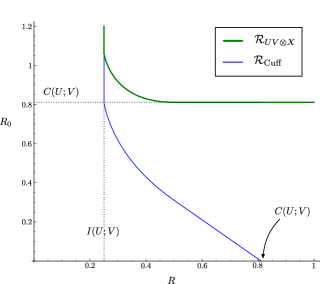
Figure 9: Comparison of the joint coordination region $\mathcal{R}_{UV\otimes X}$ with $\mathcal{R}_{\text{Cuff}}$ [12, 35]: boundaries of the regions for a binary erasure channel with erasure probability $p_{e}=0.75$ and a Bernoulli-half input.

Example 1

The difference in terms of rate of common randomness $R_{0}$ is better shown in an example: when separately coordinating the two blocks $X^{n}$ and $(U^{n},V^{n})$ without imposing a joint behavior $P_{U^{n}V^{n}X^{n}}$, the same bits of common randomness can be reused for both purposes, and the required rate $R_{0}$ is lower. We consider the case, already analyzed in [12, 35], of a Bernoulli-half source $U$, and $V$ which is an erasure with probability $p_{e}$ and is equal to $U$ otherwise. In [12] the authors prove that the optimal choice for the joint distributed $P_{UWV}$ is the concatenation of two erasure channels $\bar{P}_{W|U}$ and $\bar{P}_{V|W}$ with erasure probability $p_{1}$ and $p_{2}$ respectively. Then we have

$$p_{2}\in[0,\min\{1/2;p_{e}\}],\quad p_{1}=1-\frac{1-p_{e}}{1-p_{2}}$$

and therefore we obtain

$$I(U;W)=1-p_{1},\qquad I(UV;W)=h(p_{e})+(1-p_{1})(1-h(p_{2}))$$

where $h$ is the binary entropy function. Figure 9 shows the boundaries of the regions (55) (blue) and (56) (green) for $p_{e}=0.75$ and a Bernoulli-half input. The dotted bound $R\geq I(U;V)$ comes directly from combining $R\geq I(U;W)$ with the Markov chain $U-W-V$. At the other extreme, if $R_{0}=0$ in (55), $R+R_{0}\geq I(UV;W)\geq C(U;V)$ where $C(U;V):=\min_{U-W-V}I(U,V;W)$ is Wyner’s common information [35]. On the other hand, in our setting (56), $R_{0}\geq I(UV;W)\geq C(U;V)$ for any value of $R=H(X)$.

Moreover, note that as $R=H(X)$ tends to infinity, there is no constraint on the auxiliary random variable $W$ (aside from the Markov chain $U-V-W$) and similarly to [36] the minimum rate of common randomness $R_{0}$ needed for strong coordination is Wyner’s common information $C(U;V)$. In particular to achieve joint strong coordination of $(U,X,V)$ a positive rate of common randomness is required. The boundaries of the rate regions only coincide on one extreme, and $\mathcal{R}_{UV\otimes X}$ is strictly contained in $\mathcal{R}_{\text{Cuff}}$.

VI Polar coding schemes for strong coordination with no state and side information

Although our achievability results shed some light on the fundamental limits of coordination over noisy channels, the problem of designing practical codes for strong coordination in this setting is still open. In this section we focus on channels without state and side information for simplicity, and we show that the coordination region of Theorem 1 is achievable using polar codes, if an error-free channel of negligible rate is available between the encoder and decoder.

We note that polar codes have already been proposed for coordination in other settings: [19] proposes polar coding schemes for point-to-point empirical coordination with error free links and uniform actions, while [21] generalizes the polar coding scheme to the case of non uniform actions. Polar coding for strong point-to-point coordination has been presented in [20, 37]. In [22] the authors construct a joint coordination-channel polar coding scheme for strong coordination of actions. We present a joint source-channel polar coding scheme for strong coordination and we require joint coordination of signals and actions over a noisy channel.

For brevity, we only focus on the set of achievable distributions in $\mathcal{R}^{\prime}_{\text{in}}$ for which the auxiliary variable $W$ is binary. The scheme can be extended to the case of a non-binary random variable $W$ using non-binary polar codes [38].

Theorem 6

The subset of the region $\mathcal{R}^{\prime}_{\text{in}}$ defined in (3) for which the auxiliary random variable $W$ is binary is achievable using polar codes, provided there exists an error-free channel of negligible rate between the encoder and decoder.

To convert the information-theoretic achievability proof of Theorem 1 into a polar coding proof, we use source polarization [39] to induce the desired joint distribution. Inspired by [23], we want to translate the random binning scheme into a polar coding scheme. The key idea is that the information contraints and rate conditions found in the random binning proof directly convert into the definition of the polarization sets. In the random binning scheme we reduced the amount of common randomness $F$ by having the nodes to agree on an instance of $F$, here we recycle some common randomness using a chaining construction as in [24, 25].

Consider random vectors $U^{n}$, $W^{n}$, $X^{n}$, $Y^{n}$ and $V^{n}$ generated i.i.d. according to $\bar{P}_{UWXYV}$ that satisfies the inner bound of (3). For $n=2^{m}$, $m\in\mathbb{N}$, we note $G_{n}:=\footnotesize\begin{bmatrix}1&0\\ 1&1\end{bmatrix}^{\otimes m}$ the source polarization transform defined in [39]. Let $R^{n}:=W^{n}G_{n}$ be the polarization of $W^{n}$. For some $0<\beta<1/2$, let $\delta_{n}=2^{-n^{\beta}}$ and define the very high entropy and high entropy sets:

$$\begin{split}\operatorname{\mathcal{V}}_{W}:&=\left\{j\in\llbracket 1,n\rrbracket:H(R_{j}|R^{j-1})>1-\delta_{n}\right\},\\ \operatorname{\mathcal{V}}_{W|U}:&=\left\{j\in\llbracket 1,n\rrbracket:H(R_{j}|R^{j-1}U^{n})>1-\delta_{n}\right\},\\ \operatorname{\mathcal{V}}_{W|Y}:&=\left\{j\in\llbracket 1,n\rrbracket:H(R_{j}|R^{j-1}Y^{n})>1-\delta_{n}\right\},\\ \operatorname{\mathcal{H}}_{W|Y}:&=\left\{j\in\llbracket 1,n\rrbracket:H(R_{j}|R^{j-1}Y^{n})>\delta_{n}\right\}.\end{split}$$ (57)

Now define the following disjoint sets:

$$A_{1}:=\operatorname{\mathcal{V}}_{W|U}\cap\operatorname{\mathcal{H}}_{W|Y},\quad A_{2}:=\operatorname{\mathcal{V}}_{W|U}\cap\operatorname{\mathcal{H}}_{W|Y}^{c},$$

$$A_{3}:=\operatorname{\mathcal{V}}_{W|U}^{c}\cap\operatorname{\mathcal{H}}_{W|Y},\quad A_{4}:=\operatorname{\mathcal{V}}_{W|U}^{c}\cap\operatorname{\mathcal{H}}_{W|Y}^{c}.$$

Remark 16

We have:

• $\operatorname{\mathcal{V}}_{W|Y}\subset\operatorname{\mathcal{H}}_{W|Y}$ and $\lim_{n\rightarrow\infty}\frac{\lvert\operatorname{\mathcal{H}}_{W|Y}\setminus\operatorname{\mathcal{V}}_{W|Y}\rvert}{n}=0$ [39],

• $\lim_{n\rightarrow\infty}\frac{\lvert\operatorname{\mathcal{V}}_{W|U}\rvert}{n}=H(W|U)$ [40],

• $\lim_{n\rightarrow\infty}\frac{\lvert\operatorname{\mathcal{H}}_{W|Y}\rvert}{n}=H(W|Y)$ [39].

Since $H(W|U)-H(W|Y)=I(W;Y)-I(W;U),$ for sufficiently large $n$ the assumption $I(W;Y)\geq I(W;U)$ directly implies that $\lvert A_{2}\rvert\geq\lvert A_{3}\rvert$.

Encoding

The encoder observes $k$ blocks of the source $U^{n}_{(1:k)}:=(U^{n}_{(1)},\ldots,U^{n}_{(k)})$ and generates for each block $i\in\llbracket 1,k\rrbracket$ a random variable $\widetilde{R}^{n}_{(i)}$ following the procedure described in Algorithm 1. Similar to [2], the chaining construction proceeds as follows:

• let $A^{\prime}_{1}:=\mathcal{V}_{W|UXYV}$, observe that $A^{\prime}_{1}$ is a subset of $A_{1}$ since $\mathcal{V}_{W|UXYV}\subset\mathcal{V}_{W|U}$ and $\mathcal{V}_{W|UXYV}\subset\mathcal{V}_{W|Y}$ $\subset\mathcal{H}_{W|Y}$. The bits in $A^{\prime}_{1}\subset\operatorname{\mathcal{V}}_{W|U}$ in block $i\in\llbracket 1,k\rrbracket$ are chosen with uniform probability using a uniform randomness source $\bar{C}^{\prime}$ shared with the decoder, and their value is reused over all blocks;

• the bits in $A_{1}\setminus A^{\prime}_{1}\subset\operatorname{\mathcal{V}}_{W|U}$ in block $i\in\llbracket 1,k\rrbracket$ are chosen with uniform probability using a uniform randomness source $\bar{C}_{i}$ shared with the decoder;

• in the first block the bits in $A_{2}\subset\operatorname{\mathcal{V}}_{W|U}$ are chosen with uniform probability using a local randomness source $M$;

• for the following blocks, let $A^{\prime}_{3}$ be a subset of $A_{2}$ such that $\lvert A^{\prime}_{3}\rvert=\lvert A_{3}\rvert$. The bits of $A_{3}$ in block $i$ are sent to $A^{\prime}_{3}$ in the block $i+1$ using a one time pad with key $C_{i}$. Thanks to the Crypto Lemma [34, Lemma 3.1], if we choose $C_{i}$ of size $\lvert A_{3}\rvert$ to be a uniform random key, the bits in $A^{\prime}_{3}$ in the block $i+1$ are uniform. The bits in $A_{2}\setminus A^{\prime}_{3}$ are chosen with uniform probability using the local randomness source $M$;

• the bits in $A_{3}$ and in $A_{4}$ are generated according to the previous bits using successive cancellation encoding as in [39]. Note that it is possible to sample efficiently from $\bar{P}_{R_{i}\mid R^{i-1}U^{n}}$ given $U^{n}$ [39].

As in [23], to deal with unaligned indices, chaining also requires in the last encoding block to transmit $R_{(k)}[A_{3}]$ to the decoder. Hence the coding scheme requires an error-free channel between the encoder and decoder which has negligible rate since $\lvert R_{(k)}[A_{3}]\rvert\leq\lvert\operatorname{\mathcal{H}}_{W|Y}\rvert$ and

$$\lim_{n\rightarrow\infty\atop k\rightarrow\infty}\frac{\lvert\operatorname{\mathcal{H}}_{W|Y}\rvert}{kn}=\lim_{k\rightarrow\infty}\frac{H(W|Y)}{k}=0.$$

The encoder then computes $\widetilde{W}^{n}_{(i)}=\widetilde{R}^{n}_{(i)}G_{n}$ for $i=1,\ldots,k$ and generates $X^{n}_{(i)}$ symbol by symbol from $\widetilde{W}^{n}_{(i)}$ and $U^{n}_{(i)}$ using the conditional distribution

$$\bar{P}_{X_{j,(i)}|\widetilde{W}_{j,(i)}U_{j,(i)}}(x|\widetilde{w}_{j,(i)},u_{j,(i)})=\bar{P}_{X|WU}(x|w_{j,(i)},u_{j,(i)})$$

and sends $X^{n}_{(i)}$ over the channel.

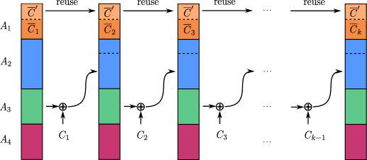
Figure 10: Chaining construction for block Markov encoding

Input :  $(U^{n}_{(1)},\ldots,U^{n}_{(k)})$, $M$ local randomness (uniform random bits), common randomness $(\bar{C}^{\prime},\bar{C}_{1:k},C_{1:k-1})$ shared with the decoder, where $\bar{C}^{\prime}$ has size $\lvert A^{\prime}_{1}\rvert$, $\bar{C}_{1:k}$ has size $k\lvert A_{1}\setminus A^{\prime}_{1}\rvert$, $C_{1:k-1}$ has size $(k-1)\lvert A_{3}\rvert$.

Output : $\left(\widetilde{R}_{(1)}^{n},\ldots,\widetilde{R}_{(k)}^{n}\right)$

if $i=1$ then

       $\widetilde{R}_{(1)}[A^{\prime}_{1}]\longleftarrow\bar{C}^{\prime}\qquad\widetilde{R}_{(1)}[A_{1}\setminus A^{\prime}_{1}]\longleftarrow\bar{C}_{1}\qquad\widetilde{R}_{(1)}[A_{2}]\longleftarrow M$

       for $j\in A_{3}\cup A_{4}$ do

             Given $U^{n}_{(1)}$, successively choose the bits $\widetilde{R}_{j,(1)}$ according to

$$\bar{P}_{R_{j}\mid R^{j-1}U^{n}}\left(\widetilde{R}_{j,(1)}\mid\widetilde{R}^{j-1}_{(1)}U^{n}_{(1)}\right)$$ (58)

       end for

      

end if

for $i=2,\ldots,k$ do

       $\widetilde{R}_{(i)}[A^{\prime}_{1}]\longleftarrow\bar{C}^{\prime}\qquad\widetilde{R}_{(i)}[A_{1}\setminus A^{\prime}_{1}]\longleftarrow\bar{C}_{i}$

       $\widetilde{R}_{(i)}[A^{\prime}_{3}]\longleftarrow\widetilde{R}_{(i-1)}[A_{3}]\oplus C_{i-1}\quad\widetilde{R}_{(i)}[A_{2}\setminus A^{\prime}_{3}]\longleftarrow M$

       for $j\in A_{3}\cup A_{4}$ do

             Given $U^{n}_{(i)}$, successively choose the bits $\widetilde{R}_{j,(i)}$ according to

$$\bar{P}_{R_{j}\mid R^{j-1}U^{n}}\left(\widetilde{R}_{j,(i)}\mid\widetilde{R}_{(i-1)}^{j}U^{n}_{(i)}\right)$$ (59)

       end for

      

end for

Algorithm 1 Encoding

Decoding

The deconding procedure described in Algorithm 2 proceeds as follows. The decoder observes $(Y^{n}_{(1)},\ldots,Y^{n}_{(k)})$ and $R_{(k)}[A_{3}]$ which allows it to decode in reverse order. We note $\widehat{R}^{n}_{(i)}$ the estimate of $R^{n}_{(i)}$ at the decoder, for $i\in\llbracket 1,k\rrbracket$. In block $i\in\llbracket 1,k\rrbracket$, the decoder has access to $\widehat{R}_{(i)}[A_{1}\cup A_{3}]=\widehat{R}_{(i)}[\operatorname{\mathcal{H}}_{W\mid Y}]$:

• the bits in $A_{1}$ in block $i$ correspond to shared randomness $\bar{C}^{\prime}$ and $\bar{C}_{i}$ for $A^{\prime}_{1}$ and $A_{1}\setminus A^{\prime}_{1}$ respectively;

• in block $i\in[1,k-1]$ the bits in $A_{3}$ are obtained by successfully recovering $A_{2}$ in block $i+1$.

Rate of common randomness

The rate of common randomness is $I(W;UXV|Y)$ since:

$$\lim_{n\to\infty}\frac{k\lvert A_{1}\rvert-(k-1)\lvert A^{\prime}_{1}\rvert+(k-1)\lvert A_{3}\rvert}{kn}=\lim_{n\to\infty}\frac{\lvert A_{1}\rvert+\lvert A_{3}\rvert-\lvert A^{\prime}_{1}\rvert}{n}$$

$$=H(W|Y)-H(W|UXYV)=I(W;UXV|Y).$$

Input : $(Y^{n}_{(1)},\ldots,Y^{n}_{(k)})$, $R_{(k)}[A_{3}]$ shared with the encoder, common randomness $(\bar{C}^{\prime},\bar{C}_{1:k-1},C_{1:k-1})$ shared with the encoder, where $\bar{C}^{\prime}$ has size $\lvert A^{\prime}_{1}\rvert$, $\bar{C}_{1:k}$ has size $k\lvert A_{1}\setminus A^{\prime}_{1}\rvert$ and $C_{1:k-1}$ has size $(k-1)\lvert A_{3}\rvert$.

Output : $(\widehat{R}_{(1)}^{n},\ldots,\widehat{R}_{(k)}^{n})$

for $i=k,\ldots,1$ do

       $\widehat{R}_{(i)}[A^{\prime}_{1}]\longleftarrow\bar{C}^{\prime}\qquad\widehat{R}_{(i)}[A_{1}\setminus A^{\prime}_{1}]\longleftarrow\bar{C}_{i}$

       if $i=k$ then

            $\widehat{R}_{(i)}[A_{3}]$ shared with the decoder

       end if

      else

            $\widehat{R}_{(i)}[A_{3}]\longleftarrow\widehat{R}_{(i+1)}[A^{\prime}_{3}]$

       end if

      for $j\in A_{2}\cup A_{4}$ do

             Successively choose the bits according to $\widehat{R}_{j,(i)}=\begin{cases}0\quad\mbox{if }L_{n}(Y_{(i)}^{n},R_{(i-1)}^{j})\geq 1\\ 1\quad\mbox{else}\end{cases}$

             where

$$L_{n}(Y_{(i)}^{n},R_{(i-1)}^{j})=\frac{\bar{P}_{R_{j,(i)}\mid R_{(i-1)}^{j}Y_{(i)}^{n}}\left(0\mid\widehat{R}_{(i-1)}^{j}Y_{(i)}^{n}\right)}{\bar{P}_{R_{j,(i)}\mid R_{(i-1)}^{j}Y_{(i)}^{n}}\left(1\mid\widehat{R}_{(i-1)}^{j}Y_{(i)}^{n}\right)}$$

       end for

      

end for

Algorithm 2 Decoding

Proof of Theorem 6

We note with $\tilde{P}$ the joint distribution induced by the encoding and decoding algorithm of the previous sections. The proof requires a few steps, here presented as different lemmas. The proofs are in Appendix H. First, we want to show that we have strong coordination in each block.

Lemma 13

In each block $i\in\llbracket 1,k\rrbracket$, we have

$$\operatorname{\mathbb{V}}\left(\widetilde{P}_{U^{n}_{(i)}\widetilde{W}_{(i)}^{n}X_{(i)}^{n}Y_{(i)}^{n}V_{(i)}^{n}},\bar{P}_{UWXYV}^{\otimes n}\right)\leq\delta_{n}^{(1)}$$ (60)

where $\delta_{n}^{(1)}:=2\mathbb{P}\left\{\widehat{W}_{(i)}^{n}\neq\widetilde{W}_{(i)}^{n}\right\}+\sqrt{2\log 2}\sqrt{n\delta_{n}}$.

Now, we want to show that two consecutive blocks are almost independent. To simplify the notation, we set

$$\begin{matrix}[ll]L:=U^{n}X^{n}Y^{n}W^{n}&\\ L_{i}:=U^{n}_{(i)}X_{(i)}^{n}Y_{(i)}^{n}V_{(i)}^{n}&i\in\llbracket 1,k\rrbracket\\ L_{a:b}:=U^{n}_{(a:b)}X^{n}_{(a:b)}Y^{n}_{(a:b)}V^{n}_{(a:b)}&\llbracket a,b\rrbracket\subset\llbracket 1,k\rrbracket\end{matrix}$$

Lemma 14

For $i\in\llbracket 2,k\rrbracket$, we have

$$\operatorname{\mathbb{V}}\left(\widetilde{P}_{L_{i-1:i}\bar{C}^{\prime}},\widetilde{P}_{L_{i-1}\bar{C}^{\prime}}\widetilde{P}_{L_{i}}\right)\leq\delta_{n}^{(3)}$$

where $\delta_{n}^{(3)}:=\sqrt{2\log 2}\sqrt{n\delta_{n}+2\delta_{n}^{(1)}(\log{\lvert\mathcal{U}\times\mathcal{X}\times\mathcal{W}\times\mathcal{Y}\times\mathcal{V}\rvert}-\log{\delta_{n}^{(1)}})}$ and $\delta_{n}^{(1)}$ is defined in Lemma 13.

Now that we have proven the asymptotical independence of two consecutive blocks, we use Lemma 14 to prove the asymptotical independence of all blocks. First we need an intermediate step.

Lemma 15

We have

$$\operatorname{\mathbb{V}}\left(\widetilde{P}_{L_{1:k}},\prod_{i=1}^{k}\widetilde{P}_{L_{i}}\right)\leq\sqrt{k-1}\delta_{n}^{(3)}$$

where $\delta_{n}^{(3)}$ is defined in Lemma 14.

Finally, we prove the asymptotical independence of all blocks.

Lemma 16

We have

$$\operatorname{\mathbb{V}}\left(\widetilde{P}_{L_{1:k}},\bar{P}_{UXYV}^{\otimes nk}\right)\leq\delta_{n}^{(5)}$$

where $\delta_{n}^{(5)}:=\sqrt{k}(\delta_{n}^{(3)}+\delta_{n}^{(2)})$ and $\delta_{n}^{(2)}$ and $\delta_{n}^{(3)}$ are defined in (71) and Lemma 14 respectively.

VII Conclusions and perspectives

In this paper we have developed an inner and an outer bound for the strong coordination region when the input and output signals have to be coordinated with the source and reconstruction. Despite the fact that we have fully characterized the region in some special cases in Section V, inner and outer bound differ in general on the information constraint. Closing this gap is left for future study.

The polar coding proof in Section VI, though it provides an explicit coding scheme, relies on a chaining construction over several blocks, which is not practical for delay-constrained applications. This is another issue that may be studied further.

Some important questions have not been addressed in this study and are left for future work. By coordinating signals and actions, the synthesized sequences would appear to be statistically indistinguishable from i.i.d. to an outside observer. As suggested in the example in Section V-D, this property could be exploited in a more general setting where two legitimate nodes wish to coordinate while concealing their actions from an eavesdropper who observes the signals sent over the channel.

Moreover, our results could be extended to a strategic coordination setting. This represents a scenario where the objectives of the two agents are not necessarily aligned, and has been investigated for empirical coordination in [41, 42].

Appendix A Proof of preliminary results

Proof:

We have

$$I(A_{t};A_{\sim t})=H(A_{t})-H(A)+H(A)-H(A_{t}|A_{\sim t})$$

and we prove separately that

$$H(A)-H(A_{t}|A_{\sim t})\leq f(\varepsilon),$$

$$H(A_{t})-H(A)\leq f(\varepsilon).$$

First, we need two results.

Lemma 17 ([43, Lemma 2.7])

Let $P$ and $Q$ two distributions on $\mathcal{A}$ such that $\operatorname{\mathbb{V}}(P,Q)=\varepsilon$ and $\varepsilon\leq 1/2$, then

$$\lvert H(P)-H(Q)\rvert\leq\varepsilon\log{\frac{\lvert\mathcal{A}\rvert}{\varepsilon}}.$$

Lemma 18 ([28, Lemma 3.2])

If $\operatorname{\mathbb{V}}(P_{A}P_{B|A},Q_{A}Q_{B|A})\leq\varepsilon$ then

$$\mathbb{P}\{A\in\mathcal{A}|\operatorname{\mathbb{V}}(P_{B|A=a},Q_{B|A=a})\leq\sqrt{\varepsilon}\}\geq 1-2\sqrt{\varepsilon}.$$

Now, consider the set $\mathcal{E}:=\{\mathbf{a}\in\mathcal{A}^{n-1}|\operatorname{\mathbb{V}}(P_{A_{t}|A_{\sim t}=\mathbf{a}},\bar{P}_{A})\leq\sqrt{\varepsilon}\}.$ By Lemma 18, $\mathbb{P}\{\mathcal{E}\}\geq 1-2\sqrt{\varepsilon}$.

Then, we have

$$H(A)-H(A_{t}|A_{\sim t})=H(A)-\!\!\!\!\!\!\sum_{\mathbf{a}\in\mathcal{A}^{n-1}}\!\!\!\!P_{A_{\sim t}}(\mathbf{a})H(A_{t}|A_{\sim t}=\mathbf{a})=\!\!\!\!\sum_{\mathbf{a}\in\mathcal{A}^{n-1}}\!\!\!\!\left(P_{A_{\sim t}}(\mathbf{a})H(A)\!-\!P_{A_{\sim t}}(\mathbf{a})H(A_{t}|A_{\sim t}=\mathbf{a})\right)$$

$$=\sum_{\mathbf{a}\in\mathcal{E}}\left(P_{A_{\sim t}}(\mathbf{a})H(A)-P_{A_{\sim t}}(\mathbf{a})H(A_{t}|A_{\sim t}=\mathbf{a})\right)+\sum_{\mathbf{a}\in\mathcal{E}^{c}}\left(P_{A_{\sim t}}(\mathbf{a})H(A)-P_{A_{\sim t}}(\mathbf{a})H(A_{t}|A_{\sim t}=\mathbf{a})\right)$$ (61)

$$\overset{(a)}{\leq}\sum_{\mathbf{a}\in\mathcal{E}}P_{A_{\sim t}}(\mathbf{a})\delta+\mathbb{P}\{\mathcal{E}^{c}\}\left(H(A_{t})+H(A)\right)\leq\delta+2\sqrt{\varepsilon}\left(2H(A)+\delta\right)$$

where $(a)$ comes from the fact that by Lemma 17 for $\mathbf{a}\in\mathcal{E}$

$$\lvert H(A_{t}|A_{\sim t}=\mathbf{a})-H(A)\rvert\leq\varepsilon\log{\frac{\lvert\mathcal{A}\rvert}{\varepsilon}}:=\delta.$$

Lemma 17 also implies that

$$\lvert H(A_{t})-H(A)\rvert\leq\delta.$$ (62)

Hence by (61) and (62), we have $I(A_{t};A_{\sim t})\leq 2\sqrt{\varepsilon}(2H(A)+\delta)+2\delta$. ∎

Proof:

The proof of (1) comes directly from Lemma 6:

$$\sum_{t=1}^{n}I(A_{t};A^{t-1}B_{\sim t}|B_{t})\leq\sum_{t=1}^{n}I(A_{t};A_{\sim t}B_{\sim t}|B_{t})\leq\sum_{t=1}^{n}I(A_{t}B_{t};A_{\sim t}B_{\sim t})\leq nf(\varepsilon).$$ (63)

To prove (2), we have

$$H(C|B^{n}) \geq I(A^{n};C|B^{n})=\sum_{t=1}^{n}I(A_{t};C|A^{t-1}B_{\sim t}B_{t})$$

$$=\sum_{t=1}^{n}I(A_{t};CA^{t-1}B_{\sim t}|B_{t})-\sum_{t=1}^{n}I(A_{t};A^{t-1}B_{\sim t}|B_{t})$$

$$\geq\sum_{t=1}^{n}I(A_{t};CB_{\sim t}|B_{t})-\sum_{t=1}^{n}I(A_{t};A^{t-1}B_{\sim t}|B_{t})$$

$$\overset{(a)}{\geq}\sum_{t=1}^{n}I(A_{t};CB_{\sim t}|B_{t})-nf(\varepsilon)=nI(A_{T};CB_{\sim T}|B_{T}T)-nf(\varepsilon)$$

$$=nI(A_{T};CB_{\sim T}T|B_{T})-nI(A_{T};T|B_{T})-nf(\varepsilon)$$

$$\geq nI(A_{T};CB_{\sim T}T|B_{T})-nI(A_{T}B_{T};T)-nf(\varepsilon)$$

where $(a)$ comes from Lemma 7.

∎

Appendix B Proof of Remark 7

We want to prove that there exists a fixed binning that satisfy both the conditions in Section IV-A2 and Section IV-A3. If we denote with $\mathbb{E}_{\varphi_{1}\varphi_{2}}$ and $\mathbb{E}_{\varphi_{2}}$ the expected value with respect to the random binnings, for all $\varepsilon$, there exists $\bar{n}$ such that $\forall n\geq\bar{n}$

$$\mathbb{E}_{\varphi_{1}\varphi_{2}}\left[\operatorname{\mathbb{V}}\left(\bar{P}^{\varphi_{1}\varphi_{2}}_{U^{n}S^{n}Z^{n}FC},Q_{F}Q_{C}\bar{P}_{U^{n}S^{n}Z^{n}}\right)\right]<\frac{\varepsilon}{2}$$

$$\mathbb{E}_{\varphi_{2}}[\operatorname{\mathbb{V}}(\bar{P}_{U^{n}S^{n}Z^{n}X^{n}Y^{n}V^{n}F}^{\varphi_{2}},Q_{F}\bar{P}_{U^{n}S^{n}Z^{n}X^{n}Y^{n}V^{n}})]<\frac{\varepsilon}{2}$$

which implies by Markov’s inequality

$$\mathbb{P}_{\varphi_{1}\varphi_{2}}\left\{\operatorname{\mathbb{V}}\left(\bar{P}^{\varphi_{1}\varphi_{2}}_{U^{n}S^{n}Z^{n}FC},Q_{F}Q_{C}\bar{P}_{U^{n}S^{n}Z^{n}}\right)<\varepsilon\right\}>\frac{1}{2}$$

$$\mathbb{P}_{\varphi_{2}}\{\operatorname{\mathbb{V}}(\bar{P}_{U^{n}S^{n}Z^{n}X^{n}Y^{n}V^{n}F}^{\varphi_{2}},Q_{F}\bar{P}_{U^{n}S^{n}Z^{n}X^{n}Y^{n}V^{n}})<\varepsilon\}>\frac{1}{2}.$$ (64)

In Section IV-A2 and IV-A3 we have chosen the binnings $(\varphi^{\prime}_{1},\varphi^{\prime}_{2})$ and $\varphi^{\prime\prime}_{2}$ respectively such that

$$\lim_{n\to\infty}\operatorname{\mathbb{V}}\left(\bar{P}^{\varphi^{\prime}_{1}\varphi^{\prime}_{2}}_{U^{n}S^{n}Z^{n}FC},Q_{F}Q_{C}\bar{P}_{U^{n}S^{n}Z^{n}}\right)=0$$

$$\lim_{n\to\infty}\operatorname{\mathbb{V}}(\bar{P}^{\varphi^{\prime\prime}_{2}}_{U^{n}S^{n}Z^{n}X^{n}Y^{n}V^{n}F},Q_{F}\bar{P}_{U^{n}S^{n}Z^{n}X^{n}Y^{n}V^{n}})=0.$$

It follows from (64) that the intersection of the two sets is non-empty, therefore there exists a binning $\varphi_{2}^{*}$ that satisfies both conditions. ∎

Appendix C Comparison between $I(XUS;YZ)$ and $I(XS;Y)+I(U;Z)$

Observe that

$$I(XUS;YZ) =I(XS;YZ)+I(U;YZ|XS)$$

$$\overset{(a)}{=}I(XS;Y)+I(U;Z)+I(SXY;Z)-I(Y;Z)+I(UZ;SXY)-I(SXY;Z)-I(U;XS)$$

$$\overset{(b)}{=}I(XS;Y)+I(U;Z)-I(Y;Z)+I(UZ;SX)-I(U;XS)$$

$$=I(XS;Y)+I(U;Z)-I(Y;Z)+I(Z;SX|U)+I(U;XS)-I(U;XS)$$

$$\overset{(c)}{=}I(XS;Y)+I(U;Z)-I(Y;Z)+I(Z;S|U)$$

where $(a)$ follows from basic properties of the mutual information, $(b)$ and $(c)$ from the Markov chains $Y-XS-UZ$ and $X-US-Z$ respectively. If we note $\Delta:=I(Z;S|U)-I(Y;Z)$, then $I(XUS;YZ)=I(XS;Y)+I(U;Z)+\Delta$ where $\Delta$ may be either positive or negative, for instance:

• in the special case where $S-U-Z$ holds and $Y=Z$, $\Delta=-H(Y)\leq 0$,

• if we suppose $Y$ independent of $Z$, $\Delta=I(Z;S|U)\geq 0$.

∎

Appendix D Proof of Lemma 11.

To prove that $I(Y_{t}{Z}_{t};C,X_{\sim t}U_{\sim t}S_{\sim t}Y_{\sim t}{Z}_{\sim t}|X_{t}U_{t}S_{t})=0$, we have

$$I(Y_{t}{Z}_{t};CX_{\sim t}S_{\sim t}U_{\sim t} Y_{\sim t}{Z}_{\sim t}|X_{t}S_{t}U_{t})$$

$$=I({Z}_{t};CX_{\sim t}S_{\sim t}U_{\sim t}Y_{\sim t}{Z}_{\sim t}|X_{t}S_{t}U_{t})+I(Y_{t};CX_{\sim t}S_{\sim t}U_{\sim t}Y_{\sim t}{Z}_{\sim t}|X_{t}S_{t}U_{t}{Z}_{t})$$

$$=I({Z}_{t};CX_{t}X_{\sim t}S_{\sim t}U_{\sim t}Y_{\sim t}{Z}_{\sim t}|S_{t}U_{t})-I({Z}_{t};X_{t}|S_{t}U_{t})$$

$$\quad+I(Y_{t};CU_{t}{Z}_{t}X_{\sim t}S_{\sim t}U_{\sim t}Y_{\sim t}{Z}_{\sim t}|X_{t}S_{t})-I(Y_{t};U_{t}{Z}_{t}|X_{t}S_{t})$$

$$\leq I({Z}_{t};CX^{n}S_{\sim t}U_{\sim t}Y_{\sim t}{Z}_{\sim t}|S_{t}U_{t})+I(Y_{t};CU^{n}Z^{n}X_{\sim t}S_{\sim t}Y_{\sim t}|X_{t}S_{t})$$

$$\leq I({Z}_{t};CX^{n}Y^{n}S_{\sim t}U_{\sim t}{Z}_{\sim t}|S_{t}U_{t})+I(Y_{t};CU^{n}Z^{n}X_{\sim t}S_{\sim t}Y_{\sim t}|X_{t}S_{t})$$

where both $I({Z}_{t};CX^{n}Y^{n}S_{\sim t}U_{\sim t}{Z}_{\sim t}|S_{t}U_{t})$ and $I(Y_{t};CU^{n}Z^{n}X_{\sim t}S_{\sim t}Y_{\sim t}|X_{t}S_{t})$ are equal to zero because by (14) the following Markov chains hold:

$${Z}_{t}-(U_{t},S_{t})-(C,X^{n},Y^{n},U_{\sim t},S_{\sim t},{Z}_{\sim t}),\qquad Y_{t}-(X_{t},S_{t})-(C,Z^{n},U^{n},X_{\sim t},S_{\sim t},Y_{\sim t}).$$

∎

Appendix E Proof of (45)

Define the event of error $E$ as follows:

$$E:=\begin{cases}0\quad\mbox{ if }\quad U^{n}=V^{n}\\ 1\quad\mbox{ if }\quad U^{n}\neq V^{n}\end{cases}.$$

We note $p_{e}:=\mathbb{P}\{U^{n}\neq V^{n}\}$ and recall that by hypothesis the distribution $P_{U^{n}S^{n}Z^{n}X^{n}Y^{n}V^{n}}$ is $\varepsilon$-close in total variational distance to the i.i.d. distribution $\bar{P}_{USZXYV}^{\otimes n}$ where the decoder is lossless. Then $\mathbb{V}(P_{V^{n}},\mathds{1}_{V=U}^{\otimes n})<\varepsilon$ and therefore $p_{e}$ vanishes. By Fano’s inequality [44], we have

$$H(U^{n}|C,Y^{n},Z^{n})\leq H_{2}(p_{e})+p_{e}\log{(\lvert\mathcal{U}^{n}\rvert-1)}.$$ (65)

Since $p_{e}$ vanishes, $H_{2}(p_{e})$ is close to zero and the right-hand side of (65) goes to zero. Hence, we have that $H(U^{n}|C,Y^{n},Z^{n})\leq nf(\varepsilon)$, where $f(\varepsilon)$ denotes a function which tends to zero as $\varepsilon$ does. ∎

Appendix F Proof of Proposition 2

F-A Achievability

We show that $\mathcal{R}_{UV\otimes X}$ is contained in the region $\mathcal{R}_{\text{PC}}\cap\mathcal{R}_{\text{SEP}}$ and thus it is achievable.

We consider the subset of $\mathcal{R}_{\text{SEP}}$ when $\bar{P}_{Y|X}(\mathbf{y}|\mathbf{x})={\mathds{1}}_{X=Y}\{\mathbf{x}=\mathbf{y}\}$ as the union of all $\mathcal{R}_{\text{SEP}}(W)$ with $W=(W_{1},W_{2})$ that satisfies

$$\bar{P}_{UW_{1}W_{2}XV}=\bar{P}_{U}\bar{P}_{W_{2}|U}\bar{P}_{V|W_{2}}\bar{P}_{X}\bar{P}_{W_{1}|X},$$

$$I(W_{1};X)\geq I(W_{2};U),$$ (66)

$$R_{0}\geq I(W_{2};UV).$$

Similarly, $\mathcal{R}_{\text{PC}}$ is the union of all $\mathcal{R}_{\text{PC}}(W)$ with $W$ that satisfies

$$\bar{P}_{UWXV}=\bar{P}_{U}\bar{P}_{W|U}\bar{P}_{X|UW}\bar{P}_{V|WX},$$

$$H(X)\geq I(WX;U),$$ (67)

$$R_{0}\geq I(W;UV|X).$$

If we choose $W=(W_{1},W_{2})$ and we add the hypothesis that $(W_{2},U,V)$ is independent of $(W_{1},X)$, (67) becomes

$$\bar{P}_{UW_{1}W_{2}XV}=\bar{P}_{U}\bar{P}_{W_{2}|U}\bar{P}_{V|W_{2}}\bar{P}_{W_{1}}\bar{P}_{X|W_{1}},$$

$$H(X)\geq I(W_{1}W_{2}X;U)=I(W_{2};U),$$ (68)

$$R_{0}\geq I(W_{1}W_{2};UV|X)=I(W_{2};UV).$$

Note that if we identify $X=W_{1}$, we have $H(X)=I(W_{1};X)$ and $\bar{P}_{W_{1}}\bar{P}_{X|W_{1}}=\bar{P}_{X}\bar{P}_{W_{1}|X}=\bar{P}_{X}{\mathds{1}}_{X=W_{1}}$. Then, there exists a subset of $\mathcal{R}_{\text{SEP}}$ and $\mathcal{R}_{\text{PC}}$ defined as the union over all $W_{2}$ such that

$$\bar{P}_{UW_{2}XV}=\bar{P}_{U}\bar{P}_{W_{2}|U}\bar{P}_{V|W_{2}}\bar{P}_{X},$$

$$H(X)\geq I(W_{2};U),$$ (69)

$$R_{0}\geq I(W_{2};UV).$$

Finally, observe that, by definition of the region (56), $\mathcal{R}_{UV\otimes X}$ is the union over all the possible choices for $W_{2}$ that satisfy (69) and therefore $\mathcal{R}_{UV\otimes X}\subseteq\mathcal{R}_{\text{PC}}\cap\mathcal{R}_{\text{SEP}}$.

F-B Converse

Consider a code $(f_{n},g_{n})$ that induces a distribution $P_{U^{n}X^{n}V^{n}}$ that is $\varepsilon$-close in total variational distance to the i.i.d. distribution $\bar{P}_{UV}^{\otimes n}\bar{P}_{X}^{\otimes n}$. Let $T$ be the random variable defined in Section IV-B.

Then, we have

$$nR_{0} \geq H(C)\overset{(a)}{\geq}I(U^{n}V^{n};C|X^{n})=I(U^{n}V^{n};CX^{n})-I(U^{n}V^{n};X^{n})$$

$$\overset{(b)}{\geq}I(U^{n}V^{n};CX^{n})-nf(\varepsilon)=\sum_{t=1}^{n}I(U_{t}V_{t};CX^{n}|U^{t-1}V^{t-1})-nf(\varepsilon)$$

$$=\sum_{t=1}^{n}I(U_{t}V_{t};CX^{n}U^{t-1}V^{t-1})-\sum_{t=1}^{n}I(U_{t}V_{t};U^{t-1}V^{t-1})-nf(\varepsilon)$$

$$\overset{(c)}{\geq}\sum_{t=1}^{n}I(U_{t}V_{t};CX^{n}U^{t-1}V^{t-1})-2nf(\varepsilon)\geq\sum_{t=1}^{n}I(U_{t}V_{t};CX^{n}U^{t-1})-2nf(\varepsilon)$$

$$=nI(U_{T}V_{T};CX^{n}U^{T-1}|T)-2nf(\varepsilon)=nI(U_{T}V_{T};CX^{n}U^{T-1}T)-nI(U_{T}V_{T};T)-2nf(\varepsilon)$$

$$\overset{(d)}{\geq}nI(U_{T}V_{T};CX^{n}U^{T-1}T)-3nf(\varepsilon)$$

where $(a)$ follows from basic properties of entropy and mutual information and $(b)$ from the upperbound on the mutual information in Lemma 1 since we assume $\mathbb{V}(P_{U^{n}V^{n}X^{n}},\bar{P}_{UV}^{\otimes n}\bar{P}_{X}^{\otimes n})\leq\varepsilon$ and $\lvert\mathcal{U}\times\mathcal{V}\rvert\geq 4$. Finally, since the distributions are close to i.i.d. by hypothesis, $(c)$ and $(d)$ come from Lemma 6 and [12, Lemma VI.3] respectively.

For the second part of the converse, observe that

$$0=H(X^{n})-I(X^{n};U^{n}C)-H(X^{n}|U^{n}C)\leq\sum_{t=1}^{n}H(X_{t})-\sum_{t=1}^{n}I(X^{n};U_{t}|U^{t-1}C)-H(X^{n}|U^{n}C)$$

$$\leq\sum_{t=1}^{n}H(X_{t})-\sum_{t=1}^{n}I(X^{n};U_{t}|U^{t-1}C)=\sum_{t=1}^{n}H(X_{t})-\sum_{t=1}^{n}I(X^{n}U^{t-1}C;U_{t})+\sum_{t=1}^{n}I(U^{t-1}C;U_{t})$$

$$\overset{(e)}{=}\sum_{t=1}^{n}H(X_{t})-\sum_{t=1}^{n}I(X^{n}U^{t-1}C;U_{t})=nH(X_{T}|T)-nI(X^{n}U^{T-1}C;U_{T}|T)$$

$$\leq nH(X_{T})-nI(X^{n}U^{T-1}CT;U_{T})+nI(T;U_{T})=nH(X_{T})-nI(X^{n}U^{T-1}CT;U_{T}).$$

where $(e)$ follows from the i.i.d. nature of the source $\bar{P}_{U}$.

Then, we identify the auxiliary random variable $W_{t}$ with $(C,X^{n},U^{t-1})$ for each $t\in\llbracket 1,n\rrbracket$ and $W$ with $(W_{T},T)=$ $(C,X^{n},U^{T-1},T)$. ∎

Appendix G Proof of cardinality bounds

Here we prove separately the cardinality bound for all the outer bounds in this paper. Note that since the proofs are basically identical we will prove it in the first case and then omit most details in all the other cases. First, we state the Support Lemma [29, Appendix C].

Lemma 19

Let $\mathcal{A}$ a finite set and $\mathcal{W}$ be an arbitrary set. Let $\mathcal{P}$ be a connected compact subset of probability mass functions on $\mathcal{A}$ and $P_{A|W}$ be a collection of conditional probability mass functions on $\mathcal{A}$. Suppose that $h_{i}(\pi)$, $i=1,\ldots,d$, are real-valued continuous functions of $\pi\in\mathcal{P}$. Then for every $W$ defined on $\mathcal{W}$ there exists a random variable $W^{\prime}$ with $\lvert\mathcal{W}^{\prime}\rvert\leq d$ and a collection of conditional probability mass functions $P_{A|W^{\prime}}\in\mathcal{P}$ such that

$$\sum_{w\in\mathcal{W}}P_{W}(w)h_{i}(P_{A|W}(a|w))=\sum_{w\in\mathcal{W}^{\prime}}P_{W^{\prime}}(w)h_{i}(P_{A|W^{\prime}}(a|w))\quad i=1,\ldots,d.$$

Proof:

We consider the probability distribution $\bar{P}_{U}\bar{P}_{W|U}\bar{P}_{X|UW}\bar{P}_{Y|X}\bar{P}_{V|WY}$ that is $\varepsilon$-close in total variational distance to the i.i.d. distribution. We identify $\mathcal{A}$ with $\{1,\ldots,\lvert\mathcal{A}\rvert\}$ and we consider $\mathcal{P}$ a connected compact subset of probability mass functions on $\mathcal{A}=\mathcal{U}\times\mathcal{X}\times\mathcal{Y}\times\mathcal{V}$. Similarly to [14], suppose that $h_{i}(\pi)$, $i=1,\ldots,\lvert\mathcal{A}\rvert+4$, are real-valued continuous functions of $\pi\in\mathcal{P}$ such that:

$$h_{i}(\pi)=\begin{cases}\pi(i)&\mbox{for }i=1,\ldots,\lvert\mathcal{A}\rvert-1\\ H(U)&\mbox{for }i=\lvert\mathcal{A}\rvert\\ H(UXV|Y)&\mbox{for }i=\lvert\mathcal{A}\rvert+1\\ H(Y|UX)&\mbox{for }i=\lvert\mathcal{A}\rvert+2\\ H(V|Y)&\mbox{for }i=\lvert\mathcal{A}\rvert+3\\ H(V|UXY)&\mbox{for }i=\lvert\mathcal{A}\rvert+4\\ \end{cases}.$$

Then by Lemma 19 there exists an auxiliary random variable $W^{\prime}$ taking at most $\lvert\mathcal{U}\times\mathcal{X}\times\mathcal{Y}\times\mathcal{V}\rvert+4$ values such that:

$$H(U|W)=\sum_{w\in\mathcal{W}}P_{W}(w)H(U|W\!=\!w)=\sum_{w\in\mathcal{W}^{\prime}}P_{W^{\prime}}(w)H(U|W^{\prime}\!=\!w)=H(U|W^{\prime}),$$

$$H(UXV|YW)=\sum_{w\in\mathcal{W}}P_{W}(w)H(UXV|YW\!=\!w)=\sum_{w\in\mathcal{W}^{\prime}}P_{W^{\prime}}(w)H(UXV|YW^{\prime}\!=\!w)=H(UXV|YW^{\prime}),$$

$$H(Y|UXW)=\sum_{w\in\mathcal{W}}P_{W}(w)H(Y|UXW\!=\!w)=\sum_{w\in\mathcal{W}^{\prime}}P_{W^{\prime}}(w)H(Y|UXW^{\prime}\!=\!w)=H(Y|UXW^{\prime}),$$

$$H(V|YW)=\sum_{w\in\mathcal{W}}P_{W}(w)H(V|YW\!=\!w)=\sum_{w\in\mathcal{W}^{\prime}}P_{W^{\prime}}(w)H(V|YW^{\prime}\!=\!w)=H(V|YW^{\prime}),$$

$$H(V|UXYW)=\sum_{w\in\mathcal{W}}P_{W}(w)H(V|UXYW\!=\!w)=\sum_{w\in\mathcal{W}^{\prime}}P_{W^{\prime}}(w)H(V|UXYW^{\prime}\!=\!w)=H(V|UXYW^{\prime}).$$

Then the constraints on the conditional distributions, the information constraints and the Markov chains are still verified since we can rewrite the inequalities in (4) and the Markov chains in (5) as

$$H(U)-H(U|W)\leq I(X;Y),$$

$$R_{0}\geq H(UXV|Y)-H(UXV|WY),$$

$$I(Y;UW|X)=H(Y|X)-H(Y|UXW)=0,$$

$$I(V;UX|YW)=H(V|YW)-H(V|UXYW)=0.$$

Note that we are not forgetting any constraints: to preserve $H(U)-H(U|W)\leq I(X;Y)$ we only need to fix $H(U|W)$ because the other quantities depend only on the joint distribution $P_{UXYV}$ (which is preserved). Similarly, once the distribution $\bar{P}_{UXYV}$ is preserved, the difference $H(UXV|Y)-H(UXV|WY)$ only depends on the conditional entropy $H(UXV|WY)$ and the difference $H(Y|X)-H(Y|UXW)$ only depends on $H(Y|UXW)$. ∎

Proof:

Here let $\mathcal{A}=\mathcal{U}\times\mathcal{S}\times\mathcal{Z}\times\mathcal{X}\times\mathcal{Y}\times\mathcal{V}$ and suppose that $h_{i}(\pi)$, $i=1,\ldots,\lvert\mathcal{A}\rvert+5$, are real-valued continuous functions of $\pi\in\mathcal{P}$ such that:

$$h_{i}(\pi)=\begin{cases}\pi(i)&\mbox{for }i=1,\ldots,\lvert\mathcal{A}\rvert-1\\ H(U)&\mbox{for }i=\lvert\mathcal{A}\rvert\\ H(USXV|YZ)&\mbox{for }i=\lvert\mathcal{A}\rvert+1\\ H(Y|USX)&\mbox{for }i=\lvert\mathcal{A}\rvert+2\\ H(V|YZ)&\mbox{for }i=\lvert\mathcal{A}\rvert+3\\ H(V|YZUSX)&\mbox{for }i=\lvert\mathcal{A}\rvert+4\\ H(Z|YUSX)&\mbox{for }i=\lvert\mathcal{A}\rvert+5\end{cases}.$$

By the Markov chain $Z-(U,S)-(X,Y,W)$, the mutual information $I(Z;XYW|US)$ is zero and once the distribution $\bar{P}_{USZXYV}$ is preserved, the mutual information $I(Z;XYW|US)=H(Z|US)-H(Z|USXYW)$ only depends on $H(Z|YUSX)$. Therefore there exists an auxiliary random variable $W^{\prime}$ taking at most $\lvert\mathcal{U}\times\mathcal{S}\times\mathcal{Z}\times\mathcal{X}\times\mathcal{Y}\times\mathcal{V}\rvert+5$ values such that the constraints on the conditional distributions and the information constraints are still verified. ∎

Proof:

Similarly, here let $\mathcal{A}=\mathcal{U}\times\mathcal{Z}\times\mathcal{X}\times\mathcal{V}$ and suppose that $h_{i}(\pi)$, $i=1,\ldots,\lvert\mathcal{A}\rvert+4$, are real-valued continuous functions of $\pi\in\mathcal{P}$ such that:

$$h_{i}(\pi)=\begin{cases}\pi(i)&\mbox{for }i=1,\ldots,\lvert\mathcal{A}\rvert-1\\ H(U|XZ)&\mbox{for }i=\lvert\mathcal{A}\rvert\\ H(UV|XZ)&\mbox{for }i=\lvert\mathcal{A}\rvert+1\\ H(V|XZ)&\mbox{for }i=\lvert\mathcal{A}\rvert+2\\ H(V|ZUX)&\mbox{for }i=\lvert\mathcal{A}\rvert+3\\ H(Z|UX)&\mbox{for }i=\lvert\mathcal{A}\rvert+4\end{cases}.$$

The information constraint in Theorem 3 can be written as

$$H(X)+I(W;Z|X)-I(WX;U)=H(X)+I(WX;Z)-I(Z;X)-I(WX;U)$$

$${\overset{{(a)}}{=}}H(X)-I(Z;X)+I(WX;Z)-I(WX;UZ)=H(X)-I(Z;X)+I(WX;U|Z)$$

$$=H(X)-I(Z;X)+H(U|Z)-H(U|WXZ)\geq 0$$

where $(a)$ follows from the fact that $I(WX;UZ)=I(WX;U)$ by the Markov chain $Z-U-(W,X)$. By fixing $H(UV|XZ)$ the constraint on the bound for $R_{0}$ is satisfied and similarly to the previous cases the Markov chains are still verified. Thus there exists an auxiliary random variable $W^{\prime}$ taking at most $\lvert\mathcal{U}\times\mathcal{Z}\times\mathcal{X}\times\mathcal{V}\rvert+4$ values. ∎

Proof:

For the lossless decoder, we rewrite the constraints in the equivalent characterization of the region (46) as:

$$H(U) \leq H(YZ)-H(YZ|UW),$$

$$R_{0} \geq I(W;USX|YZ)+H(U|WYZ)=H(USX|YZ)-H(USX|WYZ)+H(U|WYZ)$$

$$=H(USX|YZ)-H(USX)+H(U)+H(SX|U)-H(SX|UWYZ).$$

Then let $\mathcal{A}=\mathcal{U}\times\mathcal{S}\times\mathcal{Z}\times\mathcal{X}\times\mathcal{Y}$ and suppose that $h_{i}(\pi)$, $i=1,\ldots,\lvert\mathcal{A}\rvert+3$, are real-valued continuous functions of $\pi\in\mathcal{P}$ such that:

$$h_{i}(\pi)=\begin{cases}\pi(i)&\mbox{for }i=1,\ldots,\lvert\mathcal{A}\rvert-1\\ H(YZ|U)&\mbox{for }i=\lvert\mathcal{A}\rvert\\ H(SX|UYZ)&\mbox{for }i=\lvert\mathcal{A}\rvert+1\\ H(Y|USX)&\mbox{for }i=\lvert\mathcal{A}\rvert+2\\ H(Z|YUSX)&\mbox{for }i=\lvert\mathcal{A}\rvert+3\end{cases}.$$

and therefore there exists an auxiliary random variable $W^{\prime}$ taking at most $\lvert\mathcal{U}\times\mathcal{S}\times\mathcal{Z}\times\mathcal{X}\times\mathcal{Y}\rvert+3$ values. ∎

Proof:

For case of separation between channel and source, we consider the following equivalent characterization of the information constraints:

$$0\leq H(YZ)-H(YZ|W_{1}W_{2})-H(US)+H(US|W_{1}W_{2}),$$

$$R_{0}\geq H(USXV|YZ)-H(USXV|YZW_{1}W_{2})$$

In this case we have $W=(W_{1},W_{2})$. Let $\mathcal{A}=\mathcal{U}\times\mathcal{S}\times\mathcal{Z}\times\mathcal{X}\times\mathcal{Y}\times\mathcal{V}$ and suppose that $h_{i}(\pi)$, $i=1,\ldots,\lvert\mathcal{A}\rvert+3$, are real-valued continuous functions of $\pi\in\mathcal{P}$ such that:

$$h_{i}(\pi)=\begin{cases}\pi(i)&\mbox{for }i=1,\ldots,\lvert\mathcal{A}\rvert-1\\ H(US)&\mbox{for }i=\lvert\mathcal{A}\rvert\\ H(USXV|YZ)&\mbox{for }i=\lvert\mathcal{A}\rvert+1\\ H(V|Z)&\mbox{for }i=\lvert\mathcal{A}\rvert+2\\ H(V|UZ)&\mbox{for }i=\lvert\mathcal{A}\rvert+3\\ \end{cases}.$$

Then there exists an auxiliary random variable $W^{\prime}=(W^{\prime}_{1},W^{\prime}_{2})$ taking at most $\lvert\mathcal{U}\times\mathcal{S}\times\mathcal{Z}\times\mathcal{X}\times\mathcal{Y}\times\mathcal{V}\rvert+3$ values. ∎

Appendix H Polar coding achievability proofs

Here we prove the results used in the achievability proof of Theorem 6.

Proof:

Similarly to [2, Lemma 5], we first prove that in each block $i\in\llbracket 1,k\rrbracket$

$$\operatorname{\mathbb{D}}\left(\bar{P}_{UW}^{\otimes n}\Big{\Arrowvert}\widetilde{P}_{U^{n}_{(i)}\widetilde{W}_{(i)}^{n}}\right)=n\delta_{n}.$$ (70)

In fact, we have

$$\operatorname{\mathbb{D}}\left(\bar{P}_{UW}^{\otimes n}\Big{\Arrowvert}\widetilde{P}_{U^{n}_{(i)}\widetilde{W}_{(i)}^{n}}\right) {\overset{{(a)}}{=}}\mathbb{D}\left(\bar{P}_{UR}^{\otimes n}\Big{\Arrowvert}\widetilde{P}_{U^{n}_{(i)}\widetilde{R}_{(i)}^{n}}\right){\overset{{(b)}}{=}}\mathbb{D}\left(\bar{P}_{R^{n}|U^{n}}\Big{\Arrowvert}\widetilde{P}_{\widetilde{R}_{(i)}^{n}|U^{n}_{(i)}}\Big{|}\bar{P}_{U^{n}}\right)$$

$${\overset{{(c)}}{=}}\sum_{j=1}^{n}\mathbb{D}\left(\bar{P}_{R_{j}|R^{j-1}U^{n}}\Big{\Arrowvert}\widetilde{P}_{\widetilde{R}_{(i),j}|\widetilde{R}_{(i)}^{j-1}U_{(i)}^{n}}\Big{|}\bar{P}_{R^{j-1}U^{n}}\right)$$

$${\overset{{(d)}}{=}}\sum_{j\in A_{1}\cup A_{2}}\mathbb{D}\left(P_{R_{j}|R^{j-1}U^{n}}\Big{\Arrowvert}\widetilde{P}_{\widetilde{R}_{(i),j}|\widetilde{R}_{(i)}^{j-1}U_{(i)}^{n}}\Big{|}\bar{P}_{R^{j-1}U^{n}}\right)$$

$${\overset{{(e)}}{=}}\sum_{j\in A_{1}\cup A_{2}}\left(1-H(R_{j}\mid R^{j-1}U^{n})\right){\overset{{(f)}}{<}}\delta_{n}\lvert\mathcal{V}_{W\mid U}\rvert\leq n\delta_{n},$$

where $(a)$ comes from the invertibility of $G_{n}$, $(b)$ and $(c)$ come from the chain rule, $(d)$ comes from (58) and (59), $(e)$ comes from the fact that the conditional distribution $\widetilde{P}_{\widetilde{R}_{(i),j}|\widetilde{R}_{(i)}^{j-1}U_{(i)}^{n}}$ is uniform for $j$ in $A_{1}$ and $A_{2}$ and $(f)$ from (57). Therefore, applying Pinsker’s inequality to (70) we have

$$\operatorname{\mathbb{V}}\left(\widetilde{P}_{U^{n}_{(i)}\widetilde{W}_{(i)}^{n}},\bar{P}_{UW}^{\otimes n}\right)\leq\sqrt{2\log 2}\sqrt{n\delta_{n}}:=\delta_{n}^{(2)}\to 0.$$ (71)

Note that $X_{(i)}^{n}$ is generated symbol by symbol from $U^{n}_{(i)}$ and $\widetilde{W}_{(i)}^{n}$ via the conditional distribution $\bar{P}_{X|UW}$ and $Y_{(i)}^{n}$ is generated symbol by symbol via the channel $\bar{P}_{Y|X}$. By Lemma 3, we add first $X_{(i)}^{n}$ and then $Y_{(i)}^{n}$ and we obtain that for each $i\in\llbracket 1,k\rrbracket$,

$$\operatorname{\mathbb{V}}\!\left(\!\widetilde{P}_{U^{n}_{(i)}\widetilde{W}_{(i)}^{n}X_{(i)}^{n}Y_{(i)}^{n}},\bar{P}_{UWXY}^{\otimes n}\right)\!=\!\operatorname{\mathbb{V}}\left(\!\widetilde{P}_{U^{n}_{(i)}\widetilde{W}_{(i)}^{n}},\bar{P}_{UW}^{\otimes n}\right)\!\leq\!\delta_{n}^{(2)}$$ (72)

and therefore the left-hand side of (72) vanishes.

Observe that we cannot use Lemma 3 again because $V_{(i)}^{n}$ is generated using $\widehat{W}_{(i)}^{n}$ (i.e. the estimate of $W_{(i)}^{n}$ at the decoder) and not $\widetilde{W}_{(i)}^{n}$. By the triangle inequality for all $i\in\llbracket 1,k\rrbracket$

$$\operatorname{\mathbb{V}}\left(\widetilde{P}_{U^{n}_{(i)}\widehat{W}_{(i)}^{n}X_{(i)}^{n}Y_{(i)}^{n}},\bar{P}_{UWXY}^{\otimes n}\right)\!\!\leq\!\operatorname{\mathbb{V}}\left(\widetilde{P}_{U^{n}_{(i)}\widehat{W}_{(i)}^{n}X_{(i)}^{n}Y_{(i)}^{n}},\widetilde{P}_{U^{n}_{(i)}\widetilde{W}_{(i)}^{n}X_{(i)}^{n}Y_{(i)}^{n}}\right)\!\!+\!\operatorname{\mathbb{V}}\left(\widetilde{P}_{U^{n}_{(i)}\widetilde{W}_{(i)}^{n}X_{(i)}^{n}Y_{(i)}^{n}},\bar{P}_{UWXY}^{\otimes n}\right).$$ (73)

We have proved in (72) that the second term of the right-hand side in (73) goes to zero, we show that the first term tends to zero as well. To do so, we apply Proposition 1 to

$$\begin{matrix}[ll]A=U^{n}_{(i)}\widehat{W}_{(i)}^{n}X_{(i)}^{n}Y_{(i)}^{n}&A^{\prime}=U^{n}_{(i)}\widetilde{W}_{(i)}^{n}X_{(i)}^{n}Y_{(i)}^{n}\\ P=\widetilde{P}_{U^{n}_{(i)}\widehat{W}_{(i)}^{n}X_{(i)}^{n}Y_{(i)}^{n}}&P^{\prime}=\widetilde{P}_{U^{n}_{(i)}\widetilde{W}_{(i)}^{n}X_{(i)}^{n}Y_{(i)}^{n}}\\ \end{matrix}$$

on $\mathcal{A}=\mathcal{U}\times\mathcal{W}\times\mathcal{X}\times\mathcal{Y}$. Since it has been proven in [39] that

$$p_{e}:=\mathbb{P}\left\{\widehat{W}_{(i)}^{n}\neq\widetilde{W}_{(i)}^{n}\right\}=O(\delta_{n})$$

we find that $\operatorname{\mathbb{V}}\left(\widetilde{P}_{U^{n}_{(i)}\widehat{W}_{(i)}^{n}X_{(i)}^{n}Y_{(i)}^{n}},\widetilde{P}_{U^{n}_{(i)}\widetilde{W}_{(i)}^{n}X_{(i)}^{n}Y_{(i)}^{n}}\right)\leq 2p_{e}$ and therefore

$$\operatorname{\mathbb{V}}\left(\widetilde{P}_{U^{n}_{(i)}\widehat{W}_{(i)}^{n}X_{(i)}^{n}Y_{(i)}^{n}},\bar{P}_{UWXY}^{\otimes n}\right)\leq 2p_{e}+\delta_{n}^{(2)}=\delta_{n}^{(1)}\to 0.$$

Since $V^{n}_{i}$ is generated symbol by symbol from $\widehat{W}^{n}_{i}$ and $Y^{n}_{i}$, we apply Lemma 3 again and find

$$\operatorname{\mathbb{V}}\left(\widetilde{P}_{U^{n}_{(i)}\widehat{W}_{(i)}^{n}X_{(i)}^{n}Y_{(i)}^{n}V_{(i)}^{n}},\bar{P}_{UWXYV}^{\otimes n}\right)\leq\delta_{n}^{(1)}\to 0.$$ (74)

∎

Proof:

For $i\in\llbracket 2,k\rrbracket$, we have

$$\operatorname{\mathbb{D}}\left(\widetilde{P}_{L_{i-1:i}\bar{C}^{\prime}}\Big{\Arrowvert}\widetilde{P}_{L_{i-1}\bar{C}^{\prime}}\widetilde{P}_{L_{i}}\right) =I(L_{i-1}\bar{C}^{\prime};L_{i}){\overset{{(a)}}{=}}I(L_{i};\bar{C}^{\prime})+I(L_{i-1};L_{i}|\bar{C}^{\prime})$$

$${\overset{{(b)}}{=}}I(L_{i};\bar{C}^{\prime})=I(L_{i};\widetilde{R}_{i}[A^{\prime}_{1}]){\overset{{(c)}}{=}}\lvert A^{\prime}_{1}\rvert-H(\widetilde{R}_{i}[A^{\prime}_{1}]|L_{i})$$

$${\overset{{(d)}}{=}}\lvert A^{\prime}_{1}\rvert-H(R[A^{\prime}_{1}]|W)+\delta_{n}^{(4)}{\overset{{(e)}}{\leq}}\lvert A^{\prime}_{1}\rvert-\sum_{j\in A^{\prime}_{1}}H(R_{j}|R^{j-1}L)+\delta_{n}^{(4)}$$ (75)

$${\overset{{(f)}}{\leq}}\lvert A^{\prime}_{1}\rvert-\lvert A^{\prime}_{1}\rvert(1-\delta_{n})+\delta_{n}^{(4)}\leq n\delta_{n}+\delta_{n}^{(4)}$$

where $(a)$ comes from the chain rule, $(b)$ from the Markov chain $L_{i-1}-\bar{C}^{\prime}-L_{i}$, $(c)$ from the fact that the bits in $A^{\prime}_{1}$ are uniform. To prove $(d)$ observe that

$$H(\widetilde{R}_{i}[A^{\prime}_{1}]|L_{i})-H(R[A^{\prime}_{1}]|L) =H(\widetilde{R}_{(i)}[A^{\prime}_{1}]L_{i})-H(R[A^{\prime}_{1}]L)-H(L_{i})+H(L)$$

$${\overset{{(g)}}{\leq}}\delta_{n}^{(1)}\log{\frac{\lvert\mathcal{U}\times\mathcal{X}\times\mathcal{W}\times\mathcal{Y}\times\mathcal{V}\rvert}{\delta_{n}^{(1)}}}\!+\!\delta_{n}^{(1)}\log{\frac{\lvert\mathcal{U}\times\mathcal{X}\times\mathcal{Y}\times\mathcal{V}\rvert}{\delta_{n}^{(1)}}}$$

$$\leq 2\delta_{n}^{(1)}(\log{\lvert\mathcal{U}\times\mathcal{X}\times\mathcal{W}\times\mathcal{Y}\times\mathcal{V}\rvert}-\log{\delta_{n}^{(1)}}):=\delta_{n}^{(4)}$$

where $(g)$ comes from Lemma 17 since

$$\operatorname{\mathbb{V}}\left(\widetilde{P}_{L_{i}},\bar{P}_{UXYV}^{\otimes n}\right)\leq\operatorname{\mathbb{V}}\left(\widetilde{P}_{L_{i}\widetilde{W}_{(i)}^{n}},\bar{P}_{UWXYV}^{\otimes n}\right)\leq\delta_{n}^{(1)}$$

that vanishes as $n$ goes to infinity. Finally $(e)$ is true because conditioning does not increase entropy and $(f)$ comes by definition of the set $A^{\prime}_{1}$. Then from Pinsker’s inequality

$$\operatorname{\mathbb{V}}\left(\widetilde{P}_{L_{i-1:i}\bar{C}^{\prime}},\widetilde{P}_{L_{i-1}\bar{C}^{\prime}}\widetilde{P}_{L_{i}}\right)\leq\sqrt{2\log 2}\sqrt{n\delta_{n}+\delta_{n}^{(4)}}=\delta_{n}^{(3)}\to 0.$$ (76)

∎

Proof:

We have

$$\operatorname{\mathbb{D}}(\widetilde{P}_{L_{1:k}}\Big{\Arrowvert}\prod_{i=1}^{k}\widetilde{P}_{L_{i}}) {\overset{{(a)}}{=}}\sum_{i=2}^{k}I(L_{i};L_{1:i-1})\leq\sum_{i=2}^{k}I(L_{i};L_{1:i-1}\bar{C}^{\prime})$$

$$=\sum_{i=2}^{k}\left(I(L_{i};L_{i-1}\bar{C}^{\prime})+\sum_{j=1}^{i-2}I(L_{i};L_{i-j-1}|L_{i-j:i-1}\bar{C}^{\prime})\right)$$

$$\leq\sum_{i=2}^{k}\left(I(L_{i};L_{i-1}\bar{C}^{\prime})+\sum_{j=1}^{i-2}I(L_{i};L_{i-j-1:i-2}|L_{i-1}\bar{C}^{\prime})\right)$$

$${\overset{{(b)}}{=}}\sum_{i=2}^{k}I(L_{i};L_{i-1}\bar{C}^{\prime}){\overset{{(c)}}{\leq}}(k-1)(n\delta_{n}+\delta_{n}^{(4)})$$

where $(a)$ comes from [37, Lemma 15], $(b)$ is true because the dependence structure of the blocks gives the Markov chain $L_{i-j-1:i-2}-L_{i-1}\bar{C}^{\prime}-L_{i}$ and $(c)$ follows from (75). We conclude with Pinsker’s inequality. ∎

Proof:

By the triangle inequality

$$\begin{split}&\operatorname{\mathbb{V}}\left(\widetilde{P}_{L_{1:k}},\bar{P}_{UXYV}^{\otimes nk}\right)\leq\operatorname{\mathbb{V}}\left(\widetilde{P}_{L_{1:k}},\prod_{i=1}^{k}\widetilde{P}_{L_{i}}\right)+\operatorname{\mathbb{V}}\left(\prod_{i=1}^{k}\widetilde{P}_{L_{i}},\bar{P}_{UXYV}^{\otimes nk}\right)\end{split}$$ (77)

where the first term is smaller than $\sqrt{k-1}\delta_{n}^{(3)}$ by Lemma 15. To bound the second term, observe that

$$\begin{split}&\operatorname{\mathbb{D}}\left(\prod_{i=1}^{k}\widetilde{P}_{L_{i}}\Big{\Arrowvert}\bar{P}_{UXYV}^{\otimes nk}\right)=\operatorname{\mathbb{D}}\left(\prod_{i=1}^{k}\widetilde{P}_{L_{i}}\Big{\Arrowvert}\prod_{i=1}^{k}\bar{P}_{UXYV}^{\otimes n}\right)=\sum_{i=1}^{k}\operatorname{\mathbb{D}}\left(\widetilde{P}_{L_{i}}\Big{\Arrowvert}\bar{P}_{UXYV}^{\otimes n}\right).\end{split}$$ (78)

By the chain rule we have that $\operatorname{\mathbb{D}}\left(\widetilde{P}_{L_{i}}\Big{\Arrowvert}\bar{P}_{UXYV}^{\otimes n}\right)\leq\operatorname{\mathbb{D}}\left(\widetilde{P}_{L_{i}W_{(i)}^{n}}\Big{\Arrowvert}\bar{P}_{UWXYV}^{\otimes n}\right)$. Since $X_{(i)}^{n}$, $Y_{(i)}^{n}$ and $V_{(i)}^{n}$ are generated symbol by symbol via the conditional distributions $\bar{P}_{X|UW}$, $\bar{P}_{Y|X}$ and $\bar{P}_{V|WY}$ respectively, by Lemma 4 we have that

$$\operatorname{\mathbb{D}}\left(\widetilde{P}_{L_{i}W_{(i)}^{n}}\Big{\Arrowvert}\bar{P}_{UWXYV}^{\otimes n}\right)=\operatorname{\mathbb{D}}\left(\widetilde{P}_{U^{n}_{(i)}W_{(i)}^{n}}\Big{\Arrowvert}\bar{P}_{UW}\right).$$ (79)

Hence, we have

$$\operatorname{\mathbb{D}}\left(\prod_{i=1}^{k}\widetilde{P}_{L_{i}}\Big{\Arrowvert}\bar{P}_{UXYV}^{\otimes kn}\right)=\sum_{i=1}^{k}\operatorname{\mathbb{D}}\left(\widetilde{P}_{L_{i}}\Big{\Arrowvert}\bar{P}_{UXYV}^{\otimes n}\right){\overset{{(a)}}{\leq}}\sum_{i=1}^{k}\operatorname{\mathbb{D}}\left(\widetilde{P}_{U^{n}_{(i)}W_{(i)}^{n}}\Big{\Arrowvert}\bar{P}_{UW}^{\otimes n}\right){\overset{{(b)}}{=}}kn\delta_{n}$$

where $(a)$ follows from the chain rule and (79) and $(b)$ comes from (70).

Then, by Pinsker’s inequality, (77) becomes:

$$\operatorname{\mathbb{V}}\left(\widetilde{P}_{L_{1:k}},\bar{P}_{UXYV}^{\otimes nk}\right)\leq\sqrt{k-1}\delta_{n}^{(3)}+\sqrt{k}\delta_{n}^{(2)}\leq\sqrt{k}(\delta_{n}^{(3)}+\delta_{n}^{(2)})=\delta_{n}^{(5)}\to 0.$$

∎

References

- [1] G. Cervia, L. Luzzi, M. L. Treust, and M. R. Bloch, “Strong coordination of signals and actions over noisy channels,” in Proc. of IEEE International Symposium on Information Theory (ISIT), 2017.
- [2] G. Cervia, L. Luzzi, M. R. Bloch, and M. L. Treust, “Polar coding for empirical coordination of signals and actions over noisy channels,” in Proc. of IEEE Information Theory Workshop (ITW), 2016, pp. 81–85.
- [3] P. W. Cuff, H. H. Permuter, and T. M. Cover, “Coordination capacity,” IEEE Transactions on Information Theory, vol. 56, no. 9, pp. 4181–4206, 2010.
- [4] C. H. Bennett, P. W. Shor, J. A. Smolin, and A. V. Thapliyal, “Entanglement-assisted capacity of a quantum channel and the reverse Shannon theorem,” IEEE Transactions on Information Theory, vol. 48, no. 10, pp. 2637–2655, 2002.
- [5] E. Soljanin, “Compressing quantum mixed-state sources by sending classical information,” IEEE Transactions on Information Theory, vol. 4, no. 8, pp. 2263–2275, 2002.
- [6] G. Kramer and S. A. Savari, “Communicating probability distributions,” IEEE Transactions on Information Theory, vol. 53, no. 2, pp. 518–525, 2007.
- [7] A. Winter, “Compression of sources of probability distributions and density operators,” 2002. [Online]. Available: http://arxiv.org/abs/quant-ph/0208131
- [8] O. Gossner, P. Hernandez, and A. Neyman, “Optimal use of communication resources,” Econometrica, pp. 1603–1636, 2006.
- [9] B. Larrousse, S. Lasaulce, and M. Bloch, “Coordination in distributed networks via coded actions with application to power control,” 2015. [Online]. Available: http://arxiv.org/abs/1501.03685
- [10] M. H. Yassaee, A. Gohari, and M. R. Aref, “Channel simulation via interactive communications,” IEEE Transactions on Information Theory, vol. 61, no. 6, pp. 2964–2982, 2015.
- [11] F. Haddadpour, M. H. Yassaee, S. Beigi, A. Gohari, and M. R. Aref, “Simulation of a channel with another channel,” IEEE Transactions on Information Theory, vol. 63, no. 5, pp. 2659–2677, 2017.
- [12] P. Cuff, “Distributed channel synthesis,” IEEE Transactions on Information Theory, vol. 59, no. 11, pp. 7071–7096, 2013.
- [13] P. Cuff and C. Schieler, “Hybrid codes needed for coordination over the point-to-point channel,” in Proc. of Allerton Conference on Communication, Control and Computing, 2011, pp. 235–239.
- [14] M. Le Treust, “Joint empirical coordination of source and channel,” IEEE Transactions on Information Theory, vol. 63, no. 8, pp. 5087–5114, 2017.
- [15] S. Satpathy and P. Cuff, “Secure cascade channel synthesis,” IEEE Transactions on Information Theory, vol. 62, no. 11, pp. 6081–6094, 2016.
- [16] M. Le Treust, “Correlation between channel state and information source with empirical coordination constraint,” in Proc. of IEEE Information Theory Workshop (ITW), 2014, pp. 272–276.
- [17] ——, “Empirical coordination with two-sided state information and correlated source and state,” in Proc. of IEEE International Symposium on Information Theory (ISIT), 2015, pp. 466–470.
- [18] B. Larrousse, S. Lasaulce, and M. Wigger, “Coordinating partially-informed agents over state-dependent networks,” in Proc. of IEEE Information Theory Workshop (ITW), 2015, pp. 1–5.
- [19] R. Blasco-Serrano, R. Thobaben, and M. Skoglund, “Polar codes for coordination in cascade networks,” in Proc. of International Zurich Seminar on Communications, 2012, pp. 55–58.
- [20] M. R. Bloch, L. Luzzi, and J. Kliewer, “Strong coordination with polar codes,” in Proc. of Allerton Conference on Communication, Control and Computing, 2012, pp. 565–571.
- [21] R. A. Chou, M. R. Bloch, and J. Kliewer, “Polar coding for empirical and strong coordination via distribution approximation,” in Proc. of IEEE International Symposium on Information Theory (ISIT), 2015, pp. 1512–1516.
- [22] S. A. Obead, J. Kliewer, and B. N. Vellambi, “Joint coordination-channel coding for strong coordination over noisy channels based on polar codes,” in Proc. of Allerton Conference on Communication, Control and Computing, 2017.
- [23] R. A. Chou and M. R. Bloch, “Polar coding for the broadcast channel with confidential messages: A random binning analogy,” IEEE Transactions on Information Theory, vol. 62, no. 5, pp. 2410–2429, 2016.
- [24] S. H. Hassani and R. Urbanke, “Universal polar codes,” in Proc. of IEEE International Symposium on Information Theory (ISIT), 2014, pp. 1451–1455.
- [25] M. Mondelli, S. H. Hassani, I. Sason, and R. Urbanke, “Achieving Marton’s region for broadcast channels using polar codes,” IEEE Transactions on Information Theory, vol. 61, no. 2, pp. 783–800, 2015.
- [26] I. Csiszár, “Almost independence and secrecy capacity,” Problems of Information Transmission, vol. 32, no. 1, pp. 48–57, 1996.
- [27] P. Cuff, “Communication in networks for coordinating behavior,” Ph.D. dissertation, Stanford University, 2009.
- [28] M. H. Yassaee, M. R. Aref, and A. Gohari, “Achievability proof via output statistics of random binning,” IEEE Transactions on Information Theory, vol. 60, no. 11, pp. 6760–6786, 2014.
- [29] A. El Gamal and Y. H. Kim, Network information theory. Cambridge University Press, 2011.
- [30] R. Ahlswede and I. Csiszár, “Common randomness in information theory and cryptography - Part II: CR capacity,” IEEE Transactions on Information Theory, vol. 44, no. 1, pp. 225–240, 1998.
- [31] A. J. Pierrot and M. R. Bloch, “Joint channel intrinsic randomness and channel resolvability,” in Proc. of IEEE Information Theory Workshop (ITW), 2013, pp. 1–5.
- [32] T. Lindvall, Lectures on the Coupling Method. John Wiley & Sons, Inc., 1992. Reprint: Dover paperback edition, 2002.
- [33] M. Le Treust, “Coding theorems for empirical coordination,” Tech. Rep., 2015. [Online]. Available: https://cloud.ensea.fr/index.php/s/X9e5x8EzJfI7I4Q
- [34] M. R. Bloch and J. Barros, Physical-layer security: from information theory to security engineering. Cambridge University Press, 2011.
- [35] P. Cuff, “Communication requirements for generating correlated random variables,” in Proc. of IEEE International Symposium on Information Theory (ISIT), 2008, pp. 1393–1397.
- [36] A. Lapidoth and M. Wigger, “Conditional and relevant common information,” in IEEE International Conference on the Science of Electrical Engineering (ICSEE), 2016, pp. 1–5.
- [37] R. A. Chou, M. R. Bloch, and J. Kliewer, “Empirical and strong coordination via soft covering with polar codes,” to appear in IEEE Transactions on Information Theory. [Online]. Available: http://arxiv.org/abs/1608.08474
- [38] E. Şaşoğlu, “Polar codes for discrete alphabets,” in Proc. of IEEE International Symposium on Information Theory (ISIT), 2012, pp. 2137–2141.
- [39] E. Arıkan, “Source polarization,” in Proc. of IEEE International Symposium on Information Theory (ISIT), 2010, pp. 899–903.
- [40] R. A. Chou, M. R. Bloch, and E. Abbe, “Polar coding for secret-key generation,” IEEE Transactions on Information Theory, vol. 61, no. 11, pp. 6213–6237, 2015.
- [41] M. Le Treust and T. Tomala, “Information design for strategic coordination of autonomous devices with non-aligned utilities,” in Proc. of Allerton Conference on Communication, Control and Computing, 2016, pp. 233–242.
- [42] ——, “Persuasion with limited communication capacity,” 2017. [Online]. Available: http://arxiv.org/abs/1711.04474
- [43] I. Csiszár and J. Körner, Information theory: coding theorems for discrete memoryless systems. Cambridge University Press, 2011.
- [44] R. M. Fano, Transmission of Information: A Statistical Theory of Communications. The M.I.T. Press and John Wiley & Sons, Inc., 1961.