On the Interactive Communication Cost of the Distributed Nearest Lattice Point Problem

Abstract

We consider the problem of distributed computation of the nearest lattice point for a two dimensional lattice. An interactive two-party model of communication is considered. Algorithms with bounded, as well as unbounded, number of rounds of communication are considered. For the algorithm with a bounded number of rounds, expressions are derived for the error probability as a function of the total number of communicated bits. We observe that the error exponent depends on the lattice. With an infinite number of allowed communication rounds, the average cost of achieving zero error probability is shown to be finite.

Given a lattice  $\Lambda\subset\mathbb{R}^{n}$, and $\mathbf{x}=(x_{1},x_{2},\ldots,x_{n})\in\mathbb{R}^{n}$, the lattice point $\mathbf{y}_{v}(x)$ which minimizes the Euclidean distance $\|\mathbf{x}-\mathbf{y}\|$, $\mathbf{y}\in\Lambda$ is called the nearest lattice point to $\mathbf{x}$. The nearest lattice point problem is to find $\mathbf{y}_{v}(\mathbf{x})$ for each $\mathbf{x}\in\mathbb{R}^{n}$.

Our objective is to study the communication cost of finding the nearest lattice point in a distributed network under the assumption that $x_{i}$ is only available at node-$i$, $i=1,2,\ldots,n$, in a network of $n$ nodes. We consider an interactive communication model in which nodes exchange information according to a pre-arranged protocol. When communication ends, each node has sufficient information to determine $\mathbf{y}(\mathbf{x})$, an approximation to $\mathbf{y}_{v}(\mathbf{x})$. We restrict our work to lattices of dimension 2, since this captures most of the main geometric insights required for the analysis.

We view our problem as a distributed function computation problem, the function being the nearest lattice point to $\mathbf{x}$ and consider interactive communication protocols for the computation of this function. In an interactive protocol, a communication session is broken up into rounds and in each round a node is allowed to compute its message based on local information and all the information that it has received from other nodes in previous rounds. Interactive protocols are more powerful than one-way protocols [26].

The cost of communication for any function depends on the nature of the function, the error criterion used if an approximate solution is sought, and the correlation structure of the source. In order to pay attention to the function alone, we will assume throughout this work that the information available at each node is statistically independent. The main contributions of the paper are as follows.

1. We consider interactive protocols with a single-round as well as interactive protocols with an unbounded number of rounds.

2. For a single round protocol we develop analytic expressions for the tradeoff between rate and error probability.

3. For interactive protocols with an unbounded number of rounds, we exhibit a construction which results in zero error probability with finite average bit cost.

4. We study the dependence of the communication cost of our protocols on the lattice structure.

Since the problem of finding the nearest lattice point can be viewed as a classification problem, where a class is the Voronoi cell of a lattice point, our results are of value for distributed classification problems in general. Given the current focus on data analytics and cloud computing, the communication costs of distributed classification problems are expected to play an important role in practice.

In a companion paper [5] we have developed upper bounds for the communication complexity of constructing a specific rectangular partition for a given lattice along with a closed form expression for the error probability $P_{e}$. The partition is referred to as a Babai partition and is an approximation to the Voronoi partition for a given lattice.

The probability of an event $E$ is written $Pr(E)$ or $P_{\mathbf{X}}(E)$, when the distribution is to be emphasized. The probability density function (pdf) of $\mathbf{X}$ is denoted by $p_{\mathbf{X}}(\cdot)$. The conditional pdf of $\mathbf{X}$ given $\mathbf{Z}$ is denoted $p_{\mathbf{X}|\mathbf{Z}}(\cdot|\cdot)$. The entropy function is denoted by $H(\cdot)$, with argument being either a random variable or a probability distribution. The differential entropy function is denoted by $h(\cdot)$ with similar convention regarding its argument. If $\mathcal{B}\subset\mathbb{R}^{2}$, then we define $\mathcal{B}^{i}=\{x_{i}~{}:~{}(x_{1},x_{2})\in\mathcal{B}\}$, $i=1,2$ to be its projection on the $i$th coordinate axis.

The remainder of the paper is organized as follows. Previous work is reviewed in Sec. I, assumptions and a preliminary analysis are presented in Sec. III, the interactive model is analyzed and quantizer design is presented for a single round of communication in Sec. IV, and for an unbounded number of rounds of communication in Sec. V. Numerical results and a discussion are in Sec. VI. A summary and conclusions is provided in Sec. VII.

I Previous Work

The problem considered here is related to the following bodies of prior work: interactive communication, distributed function computation, distributed hypothesis testing and quantization, in particular, asymptotic quantization theory. We briefly review prior work in each of these areas. Loosely speaking, communication complexity is the minimum amount of communication required to achieve a specific objective, whether it be distributed compression or distributed function computation.

Two-party interactive communication is considered in a series of papers [25],[26], [27]. When worst-case complexity is considered, infinite message complexity can be as small, but no better than, the logarithm of the one-message complexity, and the one-message complexity is the logarithm of the strong chromatic number of a graph that is derived from the support set of the joint distribution of the pair of random variables. It is also shown that two messages suffice to achieve communication within a constant factor of the best possible using an infinite number of messages. For the average case, when random variables are uniformly distributed over their support set, average case communication close to the conditional entropy can be acheived using four or more messages [27].

Given a function $f$ of several variables, the communication complexity of computing $f$ in a distributed setting is considered in [35], [16]. Early information theoretic work on communication complexity for distributed function computation includes [34]. In [28] the problem of computing $f(X,Y)$ at node-$Y$ is considered and it is shown that $H_{G}(X|Y)$ bits are necessary and sufficient, where $H_{G}$ is a conditional entropy defined on $G$ the characteristic graph of $X$, $Y$ and $f$. A characterization of the two-message rate region is also provided. More recently, two terminal interactive communication is studied in considerable detail in [21], [24], and the benefit of an unbounded number of messages is demonstrated. In particular tight bounds for computing the Boolean AND function are obtained.

If $X$ and $Y$ are iid Gaussian with unit variance, with correlation coefficient $\rho$, $f(X,Y)=(X+Y)/2$, the objective is to calculate $f$ at node-$Y$, and only a single round of communication is allowed from node-$X$ to node-$Y$ then node-$X$ must send $(1/2)\log_{2}((1-\rho^{2})/4D)$ bits to achieve mean squared error distortion $D$ [34]. If $\rho=0$, the minimum rate required coincides with the rate for communicating $X/2$ with mse distortion $D$, as can be seen from the rate distortion function for the source. If the objective is to determine $(X+Y)/2$ at both nodes with mse distortion $D$, the minimum sum rate is $\log_{2}((1-\rho^{2})/4D)$, which is twice the rate required for calculating $f$ at one node. Once again, when $\rho=0$ this coincides with the minimum rate for sending $X/2$ to $Y$ and $Y/2$ to $X$, even if multiple rounds of interactive coding are allowed [30].

Our work is based on analysis techniques for quantization [4], [9],[36] some applications of which to detection problems have already appeared in [29], [3] and  [11]. More recently, the design of fine scalar quantizers for distributed function computation with a squared error distortion measure is considered in [23] and succeeding works.

II Applications

While the problem considered in this paper is of fundamental importance, it also has potential applications to emerging systems for network security and machine learning.

The need for large scale distributed systems has been noted, by security researchers, as a foil to distributed and coordinated attacks. Examples of such attacks and pre-cursors to attacks are distributed denial of service attacks  [33], distributed port scans and fragmented worms. This is enabled by the increased sophistication of attackers, who are able to commandeer multiple resources and attack a network in a distributed manner, so as to evade localized detection techniques. A common feature of these attacks is that detection requires global information. The communication cost of detecting such attacks is high and the bottleneck is the network bandwidth, which is a few orders of magnitude smaller than memory bandwidth [2]. In response, researchers have considered the design of distributed, collaborative intrusion detection systems and several survey papers on this important subject have appeared recently, e.g [32], [22].

A similar trend towards collaborative distributed systems is observed in the area of machine learning, e.g. [15]. Machine learning systems can serve as a subsystem in an intrusion detection system, but are also of interest in a host of other applications. Primitives provided in such systems include gradient and stochastic gradient descent, map-reduce (for developing divide and conquer strategies) and graph parallel primitives. The problem of reducing the communications overhead in datacenter implementations of large scale machine learning problems has been addressed in several works, e.g. [19]. As a specific example consider the design of a neural network classifier for data that is distributed across many physical locations [18]. The focus in  [18] is on understanding the statistical performance of the proposed distributed learning algorithm—there is no explicit accounting of the communication cost of the proposed algorithm. Our work aims to fill this gap.

Finally, we would like to note that when detecting an attack in a large network, the first attack is often very hard to detect. It is only after anomalous behavior is noted that an effort is made to discover the mode of the attack, after which an attack signature is obtained for preventing further spread. Thus, the availability of network data that precedes the attack is crucial for discovering the mode of an unseen attack. Such data can take the form of counts of packets with specific source, destination IP addresses, as in [13]. However, since uncompressed network logs will consume a lot of network bandwidth, it makes sense to have available a compressed representation of a network log. In the example of packet counts, lossy compression is an acceptable and necessary step in reducing the network bandwidth requirements. The emphasis on low delay is also important here. We may not have the luxury of accumulating data for a month at each sensor node, but may wish to encode data daily.

The problem considered here has applications to the above-mentioned distributed systems and our expectation is that the communication efficiencies obtained through their solution will contribute to system efficiencies.

III Lattice Setup

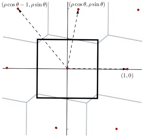
Figure 1: Voronoi region, Babai partition and three relevant vectors

Our analysis is for lattices in dimension 2. We summarize here, some of the necessary and relevant facts about two dimensional lattices. We will assume that generator matrix $\mathbf{V}$ of lattice $\Lambda$ is of full rank (the associated lattice is called a full rank lattice) and has the upper triangular form

$$\mathbf{V}=\begin{pmatrix}1&\rho\cos\theta\\ 0&\rho\sin\theta\end{pmatrix}$$ (1)

where the columns of $\mathbf{V}$ are basis vectors for the lattice. The associated quadratic form is $f(x,y)=x^{2}+2\rho\cos\theta~{}xy+\rho^{2}y^{2}$. It is known that this form is reduced if and only if $2|\rho\cos\theta|\leq 1\leq\rho^{2}$ and the three smallest values taken by $f$ over $(x,y)\in\mathbb{Z}^{2}-\{0\}$ are $1$, $\rho^{2}$, and $1-2|\rho\cos\theta|+\rho^{2}$ see e.g. Th. II, Ch. II, [7]. Based on a result due to Voronoi, Th. 10, Ch. 21, [8], it follows that the relevant vectors, i.e. the vectors which determine the faces of the Voronoi cell, are $\pm(1,0)$, $\pm(\rho\cos\theta,\rho\sin\theta)$ and $\pm(\rho\cos\theta-1,\rho\sin\theta)$. We thus consider lattices with generator matrix $\mathbf{V}$ as above, with $\rho\geq 1$. From an additional symmetry, and in order to avoid indeterminate solutions we restrict $\theta$ such that $0<\rho\cos\theta<1/2$. Performance at the endpoints $0$ and $1/2$ can be obtained by taking limits. More generally, the generator matrix of the lattice is represented by matrix $\mathbf{V}$ with $i$th column $\mathbf{v}_{i}$, $i=1,2,\ldots,n$. Thus $\Lambda=\{\mathbf{V}\mathbf{u},~{}\mathbf{u}\in\mathbb{Z}^{n}\}$. The $(i,j)$ entry of V is $v_{i,j}$, thus $\mathbf{v}_{i}=(v_{1i},v_{2i},\ldots,v_{ni})$. The Voronoi cell $\mathcal{V}_{\mathbf{y}}$ is defined as the set of all $\mathbf{x}$ for which $\mathbf{y}\in\Lambda$ is the closest lattice point. When $\mathbf{y}=\mathbf{0}$, we will write $\mathcal{V}$ as shorthand for $\mathcal{V}_{\mathbf{0}}$.

A fundamental region of a lattice $\Lambda$ is a set with the property that distinct points in the set are distinct, modulo translations by lattice vectors. The volume of any fundamental region is $|\det V|$. The Voronoi cell $\mathcal{V}_{\mathbf{y}}$ is a fundamental region for the lattice $\Lambda$. For the lattice $\Lambda$ with generator matrix (1), it is not hard to show that any translate of the rectangle $[0,1)\times[0,\rho\sin\theta)$ is also a fundamental region for $\Lambda$ and that these are the only axis-aligned rectangular fundamental regions for this lattice. Given a lattice $\Lambda$ and a rectangular fundamental region $\mathcal{R}$, a partition of $\mathbb{R}^{n}$ of the form $\mathcal{R}+\mathbf{y}$, $\mathbf{y}\in\Lambda$ will be referred to as a rectangular fundamental partition of $\Lambda$. A simple method for obtaining a fundamental rectangular partition is to partition $\mathbb{R}^{n}$ into rectangles for which $\mathbf{u}=(u_{1},u_{2},\ldots,u_{n})$ is constant, where

$$u_{i}=[(x_{i}-\sum_{j=i+1}^{n}v_{ij}u_{j})/v_{ii}],~{}i=n,n-1,\ldots,1,$$ (2)

($[x]$ is the nearest integer to $x$). This partition is referred to as the nearest-plane or Babai partition, the lattice point

$$\mathbf{y}_{np}(\mathbf{x})=\mathbf{V}\mathbf{u}$$ (3)

is referred to as the Babai point, the set of $\mathbf{x}$ mapped to $\mathbf{y}$ by (2) and (3) is called the Babai cell associated with $\mathbf{y}$, denoted $\mathcal{B}_{\mathbf{y}}$. The Babai cell at the origin $\mathcal{B}_{\mathbf{0}}$ is abbreviated $\mathcal{B}$.

IV Interactive, Nearest-Plane, Single Round of Communication

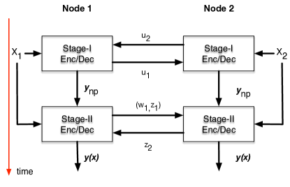
Figure 2: Two stages in the computation of $\mathbf{y}(\mathbf{x})$. At the end of Stage-I, both nodes have determined $\mathbf{y}_{np}(\mathbf{x})$. Stage-II then refines the approximation. Shown here is the 12 order for Stage-II communication. In the 21 order for Stage-II communication, $z_{2}$ is sent before $z_{1}$ and is calculated differently.

Our algorithm computes $\mathbf{y}(\mathbf{x})$ in two stages, as illustrated in Fig. 2. In the first stage, a Babai partition of $\mathbb{R}^{2}$ is constructed. This is accomplished by first sending $u_{2}$ from node-2 to node-1 and then sending $u_{1}$ from node-1 to node-2 calculated according to (2). At the conclusion of this stage of the protocol, both nodes have determined an approximate nearest lattice point, ${\mathbf{y}}_{np}(\mathbf{x})$, thus localizing $\mathbf{x}$ to the Babai cell $\mathcal{B}_{\mathbf{y}_{np}(\mathbf{x})}$. In the second stage, we allow only a single round of communication. This round consists of sending a bin index $(w_{1},z_{1})$ from node-1 to node-2 and another bin index $z_{2}$ from node-2 to node-1. Computation of $w_{1}$ and $z_{i}$’s is explained later in this section. Different results are obtained depending on the order in which the $z_{i}$ are communicated. Both possibilities are analyzed. At the end of the second stage, each node has determined a better approximation to $\mathbf{y}_{v}(\mathbf{x})$ than $\mathbf{y}_{np}(\mathbf{x})$. We call this common lattice point ${\mathbf{y}}(\mathbf{x})$.

Let $\mathcal{E}=\{\mathbf{y}(\mathbf{X})\neq\mathbf{y}_{v}(\mathbf{X})\}$ and let $P_{e}=P_{\mathbf{X}}(\mathcal{E})$ denote the error probability. The total number of bits communicated in Stages I and II is denoted by $R_{I}$, $R_{II}$, respectively and $R_{sum}=R_{I}+R_{II}$. Our objective is to determine the error probability as a function of $R_{sum}$.

Since $X_{1}$ and $X_{2}$ are assumed to be independent and the Babai cell satisfies $\mathcal{B}_{\mathbf{y}}=\mathcal{B}^{1}_{\mathbf{y}}\times\mathcal{B}^{2}_{\mathbf{y}}$, the pdf of $\mathbf{X}=(X_{1},X_{2})$ conditioned on the event $\{\mathbf{X}\in\mathcal{B}_{\mathbf{y}}\}$ or equivalently $\{\mathbf{Y}=\mathbf{y}\}$ satisfies $p_{\mathbf{X}|\mathbf{Y}}(\mathbf{x}|\mathbf{y})=p_{X_{1}|\mathbf{Y}}(x_{1}|\mathbf{y})p_{X_{2}|\mathbf{Y}}(x_{2}|\mathbf{y})$.

IV-A Analysis of Rate in Stage-I

The Stage-I rate is given by $H(\mathbf{U})$, where $\mathbf{U}=(U_{1},U_{2})$ and the $U_{i}$ are obtained in (2). For general probability distributions $H(U_{1},U_{2})$ must be obtained computationally. However, when the lattice is scaled by $\alpha$ (i.e. the generator matrix for the lattice is $\alpha\mathbf{V}$) and $\det\mathbf{V}=1$ it is easy to show that the Stage-I rate satisfies [5]

$$\lim_{\alpha\to 0}\left(R_{I}+2\log_{2}(\alpha)\right)=h(p_{X_{1}})+h(p_{X_{2}}).$$ (4)

IV-B Analysis: Stage-II, 12 Order

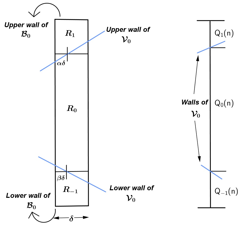
Figure 3: A typical vertical strip created by $S_{1}$ and its partition into three parts by $S_{2}$ (left). Probability distribution $Q(x)$ which underlies the calculation of $H(U_{2}|U_{1})$ is on the right.

We now describe the scheme for the $12$ order for the second stage. Node-1 partitions $\mathcal{B}^{1}$ into bins and sends a message to node-1 to indicate which bin $x_{1}$ lies in, in effect partitioning $\mathcal{B}$ into vertical rectangular strips. Node-2 partitions each vertical rectangular strip into at most three parts using at most two horizontal cuts or thresholds. The location of each cut is determined by the location of the appropriate boundary wall of a Voronoi cell. A typical situation is illustrated in Fig. 3. Here a rectangle is intersected by the boundary lines of the Voronoi cell $\mathcal{V}$, and is partitioned into three smaller rectangles. The partitioning of a rectangle into smaller rectangles is determined by the optimum decoding or decision rule, which associates a lattice point with every rectangle in the final partition. Consider a rectangle $\mathcal{R}$ and let $\mathbf{y}(\mathcal{R})$ be the lattice point that it is decoded to. From elementary considerations it follows that $\mathbf{y}(\mathcal{R})=\arg\max_{\mathbf{y}^{\prime}}P_{\mathbf{X}}(\mathcal{R}\cap\mathcal{V}_{\mathbf{y}^{\prime}})$. Thus the optimum decision rule decodes region $\mathcal{R}$ to the lattice point whose Voronoi region has the largest probability of intersection with $\mathcal{R}$.

Assume that the upper and lower boundary lines of $\mathcal{V}$ are described by $u(x)$ and $l(x)$, respectively, when $\mathbf{x}\in\mathcal{B}$. In case one or more of the Voronoi boundary lines is absent, $u(\cdot)$ and $l(\cdot)$ coincide with the boundary of the Babai cell and the slopes are zero. Let $\mathcal{R}$ have width $\delta$ and let $\alpha$ and $\beta$, both in $[0,1]$, be as shown in Fig. 3. Then

$$Pr[\mathcal{E}|\mathbf{X}\in\mathcal{R}] \approx \frac{1}{2}\delta^{2}p_{X_{1}|\mathbf{X}\in\mathcal{R}}(x_{1})\left[(\alpha^{2}+(1-\alpha)^{2})|u^{\prime}(x_{1})|p_{X_{2}|\mathbf{X}\in\mathcal{R}}(u(x_{1}))+\right.$$ (5)

$$\left.(\beta^{2}+(1-\beta)^{2})|l^{\prime}(x_{1})|p_{X_{2}|\mathbf{X}\in\mathcal{R}}(l(x_{1}))\right]$$

$$\geq \frac{1}{4}\delta^{2}p_{X_{1}|\mathbf{X}\in\mathcal{R}}(x_{1})\left[|u^{\prime}(x_{1})|p_{X_{2}|\mathbf{X}\in\mathcal{R}}(u(x_{1}))+|l^{\prime}(x_{1})|p_{X_{2}|\mathbf{X}\in\mathcal{R}}(l(x_{1}))\right]$$

and equality holds when $\alpha=\beta=1/2$. This determines the best location of two horizontal cuts for each vertical rectangular strip.

We now describe the partition of $\mathcal{B}^{1}$ in a hierarchical manner, using random variables $W_{1}$ and $Z_{1}$. The function $|u^{\prime}(x)|+|l^{\prime}(x)|$ is constant on $2m+1$ sub-intervals of $\mathcal{B}^{1}$, for some $m\geq 0$. $W_{1}$ describes the sub-interval that $X$ lies in. The sub-interval indexed by $w_{1}=0$ is special in that $|u^{\prime}(x)|+|l^{\prime}(x)|$ is zero over this sub-interval and $P(\mathcal{E}|\mathbf{U}=\mathbf{u},W_{1}=0)=0$ for each $\mathbf{u}$. No further partitioning of a sub-interval $W_{1}=0$ is required, and Stage-II communication ends. Each subinterval $W_{1}\neq 0$ is further partitioned into bins and the random variable $Z_{1}$ describes the bin index of the bin that $X_{1}$ lies in. Thus each bin is indexed by $(\mathbf{u},w_{i},i)$, where $\mathbf{u}$ is the index of the Babai cell, $w_{i}$ is the sub-interval index, $i$ is the bin index relative to the sub-interval, and

$$P_{e} = \sum_{\mathbf{u}}\sum_{w_{1}}P_{\mathbf{U},W_{1}}(\mathbf{u},w_{1})P(\mathcal{E}|\mathbf{U}=\mathbf{u},W_{1}=w_{1})$$ (6)

$$= (1-P_{W_{1}}(0))\sum_{\mathbf{u}}\sum_{w_{1}\neq 0}\frac{P_{\mathbf{U},W_{1}}(\mathbf{u},w_{1})}{(1-P_{W_{1}}(0))}P(\mathcal{E}|\mathbf{U}=\mathbf{u},W_{1}=w_{1})$$

where $P(\mathcal{E}|\mathbf{U}=\mathbf{u},W_{1}=w_{1})$ is given by averaging the minimum value achieved by (5) with appropriate bin size $\delta$.

The information rate from node-1 in Stage-II is $H(W_{1},Z_{1}|\mathbf{U})$. The sum information rate for all communication (Stages I and II) is given by

$$R_{sum}=\underbrace{H(\mathbf{U})}_{R_{I}}+\underbrace{H(Z_{1}|W_{1},\mathbf{U})+H(W_{1}|\mathbf{U})}_{R_{II,12}}+\underbrace{H(Z_{2}|Z_{1},W_{1},\mathbf{U})}_{R_{II,21}},$$ (7)

where, for convenience, we mention again that $U_{1}$ and $U_{2}$ are the random variables associated with communication in Stage-I, given by (2) and $Z_{1}$, $W_{1}$ and $Z_{2}$ are random variables associated with communication in Stage-II.

Since the quantization in Stage-II is assumed to be fine (for a lattice at any scale), we can obtain useful approximations for $H(Z_{1}|\mathbf{U},W_{1})$. Specifically, for a realization of $(\mathbf{U},W_{1})=(\mathbf{u},w_{1})$

$$H(Z_{1}|\mathbf{u},w_{1})=\sum_{i=1}^{N_{\mathbf{u},w_{1}}}\int_{\mathcal{I}_{i}}p_{X_{1}|\mathbf{U},W_{1}}(x)\log_{2}\frac{1}{\int_{\mathcal{I}_{i}}p_{X_{1}|\mathbf{U},W_{1}}(t)dt}dx,$$ (8)

where $N_{\mathbf{u},w_{1}}$, the number of bins and $\mathcal{I}_{i}$, the $i$th bin of the $w_{1}$th sub-interval of the Babai cell indexed by $\mathbf{u}$. Note that $\mathcal{I}_{i}$ may depend on $(\mathbf{u},w_{1})$ though this is not reflected in the notation.

The partition constructed by node-2 is described next. Suppose $x_{1}$ lies in the rectangle $\mathcal{R}=\mathcal{I}_{i}\times\mathcal{B}^{2}$. As shown in Fig. 3, $\mathcal{R}$ is partitioned into at most three rectangles labeled $\mathcal{R}_{j}$, $j=-1,0,1$. Define the probability distribution $Q_{\mathbf{u},w_{1}}(x_{1})=(Q_{-1},Q_{0},Q_{1})$, where $Q_{j}=P_{X_{2}|X_{1}}(R_{j}|x_{1})$. Node-2 sends $H(Z_{2}|Z_{1},\mathbf{U})$ bits to node-1 where

$$H(Z_{2}|Z_{1},\mathbf{U})\approx\sum_{\mathbf{u}}\sum_{j}P_{\mathbf{U},W_{1}}(\mathbf{u},j)\sum_{i=1}^{N_{\mathbf{u},j}}H(Q_{\mathbf{u},w_{1}}(x_{i}))p_{\mathbf{y}}(x_{i,\mathbf{u}})\delta_{i,\mathbf{u}},$$ (9)

where $x_{i,\mathbf{u}}$ lies in the $i$th bin of the $j$th sub-interval of the Babai cell indexed by $\mathbf{u}$, having length $\delta_{i,\mathbf{u}}$.

In order to derive limiting expressions for (5)–(9), we follow the approach in [4], [9],[36] and introduce the bin-length function $\delta(x)$ and the point density function $\rho(x)=(N\delta(x))^{-1}$, where $N$ is the number of bins that a sub-interval is partitioned into and $\delta(x)$ is the length of a bin that contains $x$. Observe that $\rho(x)$ measures the density of bins at $x$ within a sub-interval and integrates to unity over that sub-interval. Wherever needed $\rho$ will be indexed by the Babai cell index $\mathbf{u}$ and sub-interval $w_{1}$.

In terms of the point density function $\rho(x)$ and

$$\gamma_{\mathbf{u},w_{1}}(x):=\frac{|u^{\prime}(x)|p_{X_{2}|\mathbf{U},W_{1}}(u(x)|\mathbf{u},w_{1})+|l^{\prime}(x)|p_{X_{2}|\mathbf{U},W_{1}}(l(x)|\mathbf{u},w_{1})}{4}$$ (10)

we obtain

$$P(\mathcal{E}|\mathbf{U}=\mathbf{u},W_{1}=w_{1}) \approx \left\{\begin{array}[]{cc}E\left[\frac{\gamma_{\mathbf{u},w_{1}}(X_{1})}{\rho_{\mathbf{u},w_{1}}(X_{1})N_{\mathbf{u},w_{1}}}\left|W_{1}=w_{1},\mathbf{U}=\mathbf{u}\right.\right],&w_{1}\neq 0\\ 0,&w_{1}=0,\end{array}\right.$$ (13)

$$H(Z_{1}|\mathbf{u},w_{1}) \approx \left\{\begin{array}[]{cc}E\left[\log\left(\frac{\rho_{\mathbf{u},w_{1}}(X_{1})N_{\mathbf{u},w_{1}}}{p_{X_{1}|\mathbf{U},W_{1}}(X_{1}|\mathbf{u},w_{1})}\right)|W_{1}=w_{1},\mathbf{U}=\mathbf{u}\right],&w_{1}\neq 0,\\ 0,&w_{1}=0,\end{array}\right.$$ (16)

and

$$\lim_{m\rightarrow\infty}H(Z_{2}|Z_{1},W_{1},\mathbf{U})=\sum_{\mathbf{u}}P_{\mathbf{U}}(\mathbf{u})\sum_{w_{1}}P_{W_{1}|\mathbf{U}}(w_{1}|\mathbf{u})E\left[H(Q_{\mathbf{u},w_{1}}(X_{1})|W_{1}=w_{1},\mathbf{U}=\mathbf{u}\right].$$ (17)

Observe that (17) does not depend on $\rho$.

We minimize $P_{e}$ with respect to the sum rate $R_{sum}$ in two steps. First we obtain a lower bound on (13) through an application of Jensen’s inequality [12],  [36], [10]. We follow this with another application of Jensen’s inequality to determine the optimal rate allocation $R(\mathbf{u},w_{1})$. Thus for $w_{1}\neq 0$

$$P(\mathcal{E}|\mathbf{U}=\mathbf{u},W_{1}=w_{1})\approx$$

$$\approx E\left[\exp\left(\log\left(\frac{\gamma_{\mathbf{u},w_{1}}(X_{1})}{\rho_{\mathbf{u},w_{1}}(X_{1})N_{\mathbf{u},w_{1}}}\right)\right)\left|W_{1}=w_{1},\mathbf{U}=\mathbf{u}\right.\right]$$

$$\geq \exp\left(E\left[\log\left(\gamma_{\mathbf{u},w_{1}}(X_{1})-\log\left(\rho_{\mathbf{u},w_{1}}(X_{1})N_{\mathbf{u},w_{1}}\right)\right)|W_{1}=w_{1},\mathbf{U}=\mathbf{u}\right]\right)$$

$$\approx \exp\left(E\left[\log\left(\gamma_{\mathbf{u},w_{1}}(X_{1})\right)|\mathbf{U}=\mathbf{u},W_{1}=w_{1}\right]\right)\exp(-H(Z_{1}|\mathbf{u},w_{1}))\exp(h(X_{1}|\mathbf{U}=\mathbf{u},W_{1}=w_{1})$$

and equality holds if and only if $\rho_{\mathbf{u},w_{1}}(x_{1})N_{\mathbf{u},w_{1}}=\gamma_{\mathbf{u},w_{1}}(x_{1})/K_{\mathbf{u},w_{1}}$, for some constant $K_{\mathbf{u},w_{1}}$. Let

$$A_{\mathbf{u},w_{1}}:=\left\{\begin{array}[]{cc}E\left[\log\left(\gamma_{\mathbf{u},w_{1}}(X_{1})\right)|\mathbf{U}=\mathbf{u},W_{1}=w_{1}\right],&w_{1}\neq 0,\\ 0,&w_{1}=0\end{array}\right.$$ (19)

and let

$$\tilde{P}(\mathbf{u},w_{1})=\frac{P_{\mathbf{U},W_{1}}(\mathbf{u},w_{1})}{(1-P_{W_{1}}(0))},~{}w_{1}\neq 0.$$ (20)

From (6) it follows that

$$P_{e} \geq (1-P_{W_{1}}(0))\sum_{\mathbf{u}}\sum_{w_{1}\neq 0}\tilde{P}(\mathbf{u},w_{1})\exp(A_{\mathbf{u},w_{1}}-H(Z_{1}|\mathbf{u},w_{1})+h(X_{1}|\mathbf{u},w_{1}))$$

$$\geq (1-P_{W_{1}}(0))\exp\left(\sum_{\mathbf{u}}\sum_{w_{1}\neq 0}\tilde{P}(\mathbf{u},w_{1})\left(A_{\mathbf{u},w_{1}}-H(Z_{1}|\mathbf{u},w_{1})+h(X_{1}|\mathbf{u},w_{1})\right)\right)$$

$$\geq (1-P_{W_{1}}(0))\exp\left(\sum_{\mathbf{u}}\sum_{w_{1}\neq 0}\tilde{P}(\mathbf{u},w_{1})\left(A_{\mathbf{u},w_{1}}+h(X_{1}|\mathbf{u},w_{1})\right)\right)\exp\left(-\frac{H(Z_{1}|\mathbf{U},W_{1})}{(1-P_{w_{1}}(0))}\right)$$

and equality holds when $H(Z_{1}|\mathbf{u},w_{1})=A_{\mathbf{u},w_{1}}+h(X_{1}|\mathbf{u},w_{1})+K$ for some constant $K$. From here it follows directly that

$$\lim_{R_{sum}\rightarrow\infty}\log\left(P_{e}e^{\frac{R_{sum}}{(1-P_{W_{1}}(0))}}\right)=$$ (22)

$$\log(1-P_{W_{1}}(0))+\tilde{E}[\log\gamma_{\mathbf{U},W_{1}}+h(X_{1}|\mathbf{u},w_{1})]+\frac{H(W_{1}|\mathbf{U})}{1-P_{W_{1}}(0)}+\frac{H(\mathbf{U})+H(Z_{2}|Z_{1},\mathbf{U},W_{1})}{1-P_{W_{1}}(0)},$$

where $\tilde{E}[\cdot]$ is the expectation with respect to the probability distribution $\tilde{P}$ defined in (20) and $h(X_{1}|\mathbf{u},w_{1})$ is the differential entropy of the probability density $p_{X_{1}|\mathbf{U},W_{1}}(x|\mathbf{u},w_{1})$.

Remark 1.

From (6) we see that in order to achieve $P_{e}=0$ it is necessary that $P(\mathcal{E}|\mathcal{R}(\mathbf{u},j,i))=0$ for all $\mathcal{R}(\mathbf{u},j,i)$ which have positive probability. This is impossible unless the bin size (the $x_{1}$ dimension) is zero, which requires an infinite rate.

Remark 2.

Conditions for convergence in (22) are less stringent than those required in the analysis of quantizers under difference distortion measures since the error measure considered here is the error probability. It suffices to assume that the marginal pdf’s satisfy smoothness conditions (53(a)-(c)) in [9].

IV-C Special Case: 12 Order and $\mathbf{X}\sim\mbox{Unif}(\mathcal{B}_{\mathbf{0}})$

Figure 4: Babai and Voronoi cells, with key points labeled. $x_{1},x_{2}$ are the horizontal, vertical coordinates, resp. We have reduced the clutter by labeling only one of a pair of vertices $\mathbf{x}$, $-\mathbf{x}$.

We now specialize the analysis to the simplest case where we assume that $\mathbf{X}$ is uniformly distributed over $\mathcal{B}_{\mathbf{0}}$. Thus $H(\mathbf{U})=0$ in (22) and the remaining terms are derived in the sequel. We note here that this analysis also applies in a limiting sense when applied to lattice $\alpha\Lambda$ and $\alpha\to 0$. The only modification required is that $H(\mathbf{U})$ be computed using (4). Thus the analysis presented here is applicable in the limiting case for general source distributions. The benefit is that it allows us to study explicity, the dependence on geometric parameters of the Babai and Voronoi cell.

The Voronoi cell $\mathcal{V}_{\mathbf{0}}$ and Babai cell $\mathcal{B}_{\mathbf{0}}$ are shown with all the significant boundary points and intervals in Fig. 4. We identify four thresholds $t_{-2}=(\rho\cos\theta-1)/2$, $t_{-1}=(-\rho\cos\theta)/2$, $t_{1}=-t_{-1}$ and $t_{2}=-t_{-2}$ and five intervals $I_{-2}=(-1/2,t_{-2}]$, $I_{-1}=(t_{-2},t_{-1}]$, $I_{0}=(t_{-1},t_{1}]$, $I_{1}=(t_{1},t_{2}]$ and $I_{2}=(t_{2},1/2]$ with lengths $L_{-2}=L_{2}=(1/2)\rho\cos\theta$, $L_{-1}=L_{1}=1/2-\rho\cos\theta$, $L_{0}=\rho\cos\theta$, $L=L_{0}+2L_{1}+2L_{2}=1$. Let $H_{-2}=H_{2}=(1/2)\cos\theta/\sin\theta$. Note that $H_{-2}=H_{-2u}+H_{-2l}$ in Fig. 4. Let $H_{-1}=H_{1}=\cos\theta(1-2\rho\cos\theta)/2\sin\theta$. Note that $H_{-1}=H_{-1l}$ in Fig. 4. Let the height of the Babai cell be $H=\rho\sin\theta$. Thus

$$\gamma_{{\mathbf{0}},w_{1}}(x)=\left\{\begin{array}[]{cc}\frac{H_{-2}}{4L_{-2}H}=1/(4\rho^{2}\sin^{2}\theta),&x\in I_{-2}(\equiv w_{1}=-2)\\ \frac{H_{-1}}{4L_{-1}H}=\cos\theta/(4\rho\sin^{2}\theta),&x\in I_{-1}(\equiv w_{1}=-2)\\ 0,&x\in I_{0}(\equiv w_{1}=0)\\ \frac{H_{1}}{4L_{1}H}=\cos\theta/(4\rho\sin^{2}\theta),&x\in I_{1}(\equiv w_{1}=1)\\ \frac{H_{2}}{4L_{2}H}=1/(4\rho^{2}\sin^{2}\theta),&x\in I_{2}(\equiv w_{1}=2),\end{array}\right.$$

Then

$$\tilde{E}[\log\gamma_{\mathbf{U},W_{1}}]=\sum_{j=-2,j\neq 0}^{2}\frac{L_{j}}{1-L_{0}}\log\frac{H_{j}}{4HL_{j}}$$ (23)

$$H(W_{1}|\mathbf{U})=-\sum_{j=-2}^{2}L_{j}\log L_{j}$$ (24)

and

$$\tilde{E}[h(X_{1}|\mathbf{u},w_{1})]=\sum_{j=-2,j\neq 0}^{2}\frac{L_{j}}{1-L_{0}}\log L_{j}$$ (25)

Let random variable $W_{2}$ which takes values $j=-2,-1,0,1,2$ with probability $H_{j}/H$. We thus obtain

$$P_{e}\exp\left(\frac{R_{sum}}{1-P_{W_{1}}(0)}\right)=$$ (26)

$$= \frac{(1-P_{W_{1}}(0))}{4}\left(\frac{1}{P_{W_{1}}(0)}\right)^{\frac{P_{W_{1}}(0)}{1-P_{W_{1}}(0)}}\left(\prod_{j=-2,j\neq 0}^{2}\left(\frac{P_{W_{2}}(0)}{P_{W_{1}}(0)}\right)^{\frac{P_{W_{1}}(0)}{1-P_{W_{1}}(0)}}\right)\exp\left\{\frac{E[H(Q(X_{1}))]}{(1-P_{W_{1}}(0))}\right\}$$

$$= \frac{(1-L_{0})}{4}\left(\frac{1}{L_{0}}\right)^{\frac{L_{0}}{1-L_{0}}}\left(\prod_{j=-2,j\neq 0}^{2}\left(\frac{H_{j}}{L_{j}H}\right)^{\frac{L_{j}}{1-L_{0}}}\right)\exp\left\{\frac{E[H(Q(X_{1}))]}{(1-L_{0})}\right\}.$$ (27)

It is worth noting that for the special case considered here, namely, $\mathbf{X}$ uniformly distributed on $\mathcal{B}_{\mathbf{0}}$, (27) can be obtained more directly by partitioning $I_{-2}$ into $N_{2}$ equal-length intervals, $I_{-1}$ into $N_{1}$ equal-length intervals, $I_{0}$ into $1$ interval, $I_{1}$ into $N_{1}$ equal-length intervals and $I_{2}$ into $N_{2}$ equal-length intervals [31].

IV-D Interactive: Single Round, Reversed Steps, $\mathbf{X}\sim\mbox{Unif}(\mathcal{B}_{\mathbf{0}})$

Analysis is now presented for $21$ order of communication. The general formula (27) continues to apply here, but with $W_{2}$, $Z_{2}$ and $X_{2}$ replacing $W_{1}$, $Z_{1}$, and $X_{1}$, respectively. We thus derive an expression for the special case with $\mathbf{X}$ uniformly distributed on $\mathcal{B}_{\mathbf{0}}$, since this captures the essential geometric differences between the two orderings of communication in Stage-II.

The support for $X_{2}$ is partitioned into $3$ subintervals $\mathcal{J}_{0}:=(\tau_{-1},\tau_{1}]$, $\mathcal{J}_{-1}:=(-\rho\sin\theta/2,\tau_{-1}]$ and $\mathcal{J}_{1}=(\tau_{1},\rho\sin\theta/2]$ and the bin that $X_{2}$ lies in is communicated to node-1 by random variable $W_{2}$. Conditioned on $W_{2}\neq 0$, random variable $Z_{2}$ indicates a bin for interval $\mathcal{J}_{j}$, $j\neq 0$ that $X_{2}$ lies in. Also let $H=\rho\sin\theta$, the vertical ($X_{2}$) dimension of $\mathcal{B}_{\mathbf{0}}$ and $H_{i}=\mbox{length}(\mathcal{J}_{i})$, $i=-1,0,1$ as in Fig. 4.

Node-2 sends $W_{2},Z_{2}$, the index of the bin that $X_{2}$ lies in, and thus partitions $\mathcal{B}_{\mathbf{0}}$ into horizontal strips. Node-1 then partitions each horizontal strip into at most three parts using at most two vertical cuts or thresholds, referred to as the left and right thresholds, and sends $Z_{1}$ to node-2. For a given $x_{2}$, let $P_{-1}(x_{2})$ be the probability that $X_{1}$ lies to the left of the left threshold ($Z_{1}=-1$), $P_{1}(x_{2})$ the probability that $X_{1}$ lies to the right of the right threshold ($Z_{1}=1$) and $P_{0}(x_{2})$ the probability that $X_{1}$ lies in between the two thresholds ($Z_{1}=0$). Let $P(x)=(P_{-1}(x),P_{0}(x),P_{1}(x))$. Then

$$\lim_{m\rightarrow\infty}H(Z_{1}|Z_{2},W_{2},U_{1},U_{2})=E[H(P(X_{2})].$$ (28)

It follows that

$$\lim_{N\rightarrow\infty}P_{e,II}2^{R_{sum}/(1-P_{W_{2}}(0))}=\frac{1-H_{0}}{4H}\left(\frac{H}{H_{0}}\right)^{\frac{H_{0}}{1-H_{0}}}\left(\prod_{j=-1,j\neq 0}^{1}\frac{HL_{j}}{H_{j}}\right)\exp\left\{\frac{E[H(P(X_{2}))]}{(1-H_{0})}\right\}.$$ (29)

IV-E The Optimum Offset

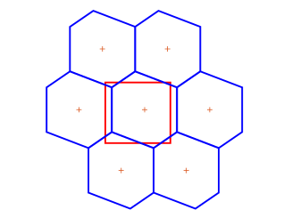
Figure 5: Shifted Babai cell (red) and Voronoi cells (blue) and lattice points ’+’. Observe that the lattice is not shifted and a lattice point remains at the center of every Voronoi cell. Also, the lattice point $\mathbf{y}$ lies in the shifted Babai cell because of our restriction on $\mathbf{x}_{0}$. A single Babai cell will intersect at most six Voronoi cells.

Figure 6: An illustration of the Voronoi cell $\mathcal{V}_{\mathbf{0}}$ an offset Babai cell (dashed rectangle) and the Babai cell with zero offset (solid rectangle).

We consider the possibility that the Babai partition constructed on $\mathbf{x}-\mathbf{x}_{0}$ for some fixed offset vector $\mathbf{x}_{0}=(x_{01},x_{02})$ might lead to improved performance. Notice that the lattice and Voronoi partition remain unchanged; only the rectangular partition has shifted. It suffices to restrict $\mathbf{x}_{0}$ to the rectangle $\prod_{i=1}^{n}[-v_{ii}/2,v_{ii}/2)$ and with this restriction $\mathbf{y}\in\mathcal{B}_{\mathbf{x}_{0}}(\mathbf{y})$. For 2D lattice considered here $\mathbf{x}_{0}\in[-1/2,1/2)\times[-(\rho/2)\cos\theta,(\rho/2)\cos\theta)$.

(a)	(b)	(c)

Figure 7: Variation with offset for $\theta=2\pi/5$ and $R_{sum}=4.0$ bits for 12 order of communication. (a) $L_{0}$ as a function of $d_{1}$, (b) $P_{e}$ given in (29) as a function of $d_{1}$ shows that $d_{1}=\rho\cos\theta(1-\rho\cos\theta)$ is optimum. (c) 21 order of communication. $P_{e}$ is minimum at zero offset.

First consider the 12 order to communication. We have already shown that the error probability decreases as $2^{-R_{sum}/(1-L_{0})}$ and thus the maximum rate of decay is obtained by choosing an offset $\mathbf{x}_{0}$ for which $L_{0}$ is maximized. In terms of the distances shown in Fig. 6, $L_{0}=1-\max(d_{1},d_{4})-\max(d_{2},d_{3})$ and $d_{1},...,d_{4}$ depend on the vertical offset $x_{02}$. For $0<d_{1}\leq\rho\cos\theta$, $d_{2}=\frac{d_{1}(1-\rho\cos\theta)}{\rho\cos\theta}$, $d_{3}=\rho\cos\theta-d_{1}$ and $d_{4}=\frac{(1-\rho\cos\theta)}{\rho\cos\theta}(\rho\cos\theta-d_{1})$. Note that offset $\mathbf{x}_{\mathbf{0}}=0$ corresponds to $d_{1}=(1/2)\rho\cos\theta$. $L_{0}$ is maximized for any $d_{1}$ which satisfies $(\rho\cos\theta)^{2}\leq d_{1}\leq\rho\cos\theta(1-\rho\cos\theta)$, as shown in Fig. 7. Thus $\mathbf{x}_{\mathbf{0}}=0$ is optimal in terms of rate of decay. A further optimization is possible in terms of the constant term. This has been calculated numerically and is shown in Fig. 7(b). For the 12 order of communication $d_{1}=\rho\cos\theta(1-\rho\cos\theta)$ is optimum (for all $\theta$ in $(\pi/3,\pi/2)$) and results in significant improvements in the error probability.

A similar, but simpler analysis for the reverse order shows that in this case the zero offset is indeed optimal, as shown in Fig. 7(c).

V Interactive: Infinite Rounds

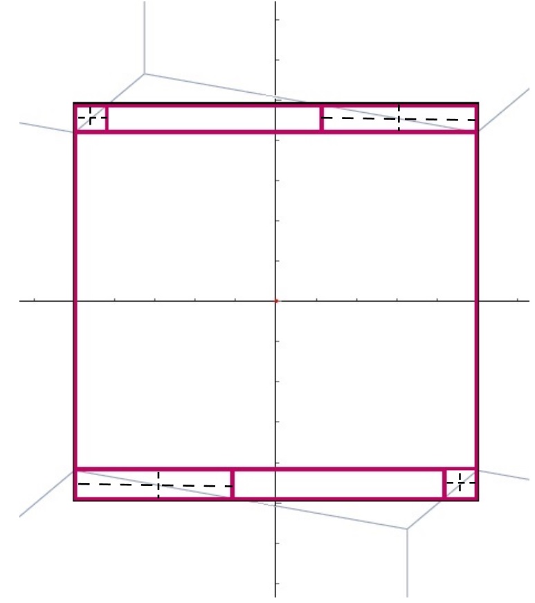
Figure 8: Red solid lines show partition after the first round of communication. Dashed lines are created in the second round of communication.

We now analyze the interactive model in which an infinite number of communication rounds are allowed. We provide an analysis under the assumption that $\mathbf{X}$ is uniformly distributed over $\mathcal{B}_{\mathbf{0}}$. As we have noted earlier, the analysis with this restriction also applies when the lattice is fine, i.e. when $|\det V|$, the volume of a fundamental region is small. The construction and performance analysis is presented is described in Sec. V-A. The optimum offset is investigated in Sec. V-B.

V-A Interactive:Infinite rounds: A Bit-Excahnge Protocol

Node-2 communicates first. In Round-1, Node-2 partitions the support of $X_{2}$ into three intervals as in Sec. IV-D (see Figs. 8 and 4), $\mathcal{J}_{-1}$, and $\mathcal{J}_{0}$, and $\mathcal{J}_{1}$. Let random variable $W_{2}$ be the index of the interval in which $X_{2}$ lies. In Round-1, upon receiving $W_{2}$ and if $W_{2}=1$, Node-1 partitions the support of $X_{1}$ into three intervals $\mathcal{I}_{-1}=(-1/2,t_{-2}]$, $\mathcal{I}_{0}=(t_{-2},t_{1}]$ and $\mathcal{I}_{1}=(t_{1},1/2]$ (see Fig. 4). If $W_{2}=-1$, the support of $X_{2}$ is partitioned into intervals $-\mathcal{I}_{1},-\mathcal{I}_{0},-\mathcal{I}_{-1}$. If $W_{2}=0$, no partitioning step is taken. Random variable $W_{1}$ describes the interval in which $X_{1}$ lies. Let $Pr(W_{2}=i)=:Q_{i}$, $i=-1,0,1$. Let $P_{i}=Pr(W_{1}=i|W_{2}=1)$, $i=-1,0,1$. Let $Q=(Q_{0},Q_{1},Q_{2})$ and $P=(P_{0},P_{1},P_{2})$.

We assume that for every round, upon sending $U_{i}$, Node-$i$ updates $X_{i}$ by subtracting the lower endpoint of the interval that it lies in.

The partition of $\mathcal{B}_{\mathbf{0}}$ into rectangular cells after a single, and after two rounds of communication is shown in Fig. 8. Define a rectangular cell to be error-free if its interior does not contain a boundary of $\mathcal{V}_{\mathbf{0}}$. Of the seven rectangles in the partition at the conclusion of Round-1, all but four are error-free. If $\mathbf{X}=(X_{1},X_{2})$ lies in an error-free rectangle, communication halts after Round-1. Else a second round of communication occurs, during which a total of 2 bits are communicated. This process of partitioning and communication continues until each node determines that $X$ lies in an error free rectangle of the current partition. When the algorithm halts, $P_{e}=0$. Let $N(\mathbf{X})$, $R(\mathbf{X})$ denote the number of rounds, and number of bits communicated, respectively, when the algorithm halts. Let $\bar{R}=E[R(\mathbf{X})]$ and $\bar{N}=E[N(\mathbf{X})]$ denote averages over $\mathbf{X}$.

Theorem 1.

For the interactive model with unlimited rounds of communication, a nearest plane partition can be transformed into the Voronoi partition using, on average, a finite number of bits and rounds of communication. Specifically,

$$\bar{R}=H(Q)+(1-Q_{0})H(P)+4(1-P_{0})(1-Q_{0})$$ (30)

and

$$\bar{N}=1+2(1-P_{0})(1-Q_{0}).$$

Proof.

We assume that an optimum entropy code is used (thus if $W_{2}=0$, the codeword length is $\log_{2}(1/Q_{0})$ bits). The term $H(Q)+(1-Q_{0})H(P)$ in (30) is the cost of resolving the Round-1 partition. At the conclusion of Round-1, if $\mathbf{X}$ belongs to a region which is not error-free, then the average number of bits transmitted is obtained by the following argument. At the conclusion of Round-1, there are two kinds of error rectangles, determined by the sign of the slope of the boundary of $\mathcal{V}_{\mathbf{0}}$ in the rectangle. Note that error rectangles are designed so that the boundary of $\mathcal{V}_{\mathbf{0}}$ is a diagonal of the corresponding rectangle. Let an error rectangle have length $L$ and height $H$. If the slope is positive, construct the binary expansion $1-x_{1}/L=\sum_{i=1}^{\infty}b_{i}2^{-i}$, else construct $x_{1}/L=\sum_{i=1}^{\infty}b_{i}2^{-i}$. In both cases construct the binary expansion $x_{2}/H=\sum_{i=1}^{\infty}c_{i}2^{-i}$. From the independence and uniformity of $X_{1}$ and $X_{2}$ it follows that the bits $B_{i}$ and $C_{i}$ are independent unbiased Bernoulli random variables. Further, the algorithm halts after $n$ rounds, with $2n$ total bits communicated if and only if $B_{i}\neq C_{i}$, $i<n$ and $B_{n}=C_{n}$. Thus, given $\mathbf{X}$ in an error rectangle, $Pr(R(\mathbf{X})=2n)=Pr(N(\mathbf{X})=n)=2^{-n}$. The result follows immediately by computing the average. ∎

V-B Infinite Rounds: Optimum Offset for the Babai Partition

With reference to Fig. 6, define the probability distributions $Q=[Q_{-1},Q_{0},Q_{1}]$, with $Q_{i}=H_{i}/H$, $i\neq 0$, $Q_{0}=(1-(Q_{1}+Q_{-1})$, $P_{1}=[P_{1,-1},P_{1,0},P_{1,1}]=[d_{1}/L,1-(d_{1}+d_{2})/L,d_{2}/L]$ and $P_{-1}=[P_{-1,-1},P_{-1,0},P_{-1,1}]=[d_{4}/L,(1-(d_{4}+d_{3})/L,d_{3}/L]$. In terms of parameters for the basis, $H=\rho\sin\theta$, $L=1$, $H_{1}=d_{1}(1-\rho\cos\theta)/(\rho\sin\theta)$, $H_{-1}=d_{3}(1-\rho\cos\theta)/(\rho\sin\theta)$ and for $0<d_{1}\leq\rho\cos\theta$, $d_{2}=\frac{d_{1}(1-\rho\cos\theta)}{\rho\cos\theta}$, $d_{3}=\rho\cos\theta-d_{1}$ and $d_{4}=\frac{(1-\rho\cos\theta)}{\rho\cos\theta}(\rho\cos\theta-d_{1})$ (replicated here for convenience).

The sum rate for Stage-II communication is given by

$$R_{II}=H(Q)+Q_{1}H(P_{1})+Q_{-1}H(P_{-1})+(Q_{1}(1-P_{1,0})+Q_{-1}(1-P_{-1,0}))4$$ (31)

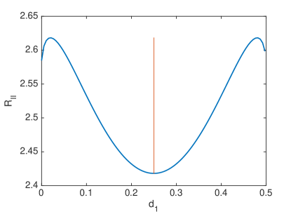
Figure 9: Variation of rate with $d_{1}$ shows that zero offset is optimum for 21 order infinite round communication for $\rho=1$ and $\theta=2\pi/5$. The vertical line shows $d_{1}$ at zero offset.

The sum rate plotted in in Fig. 9, for the offset Babai partition shows that zero offset is optimal, consistent with the result for the 21 single-round result.

Remark 3.

The communication strategy is implicit in the proof. Note that the finite value for $\bar{R}$ is because of the rapid decrease with $n$ of the probability of halting at $n$ rounds.

Remark 4.

This result has interesting implications when viewed in the context of distributed classification problems. Suppose we have an optimum two-dimensional classifier with separating boundaries that are not axis aligned and also a suboptimal classifier with separating boundaries that are axis aligned, e.g. a $k$-$d$ tree. We expect the communication complexity of refining the approximate rectangular classifier to the optimum classifier to be finite.

VI Numerical Results and Discussion

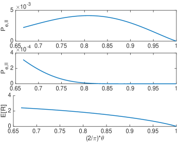
Figure 10: Variation of $P_{e,II}$ with $\theta$ for the single-round interactive model, 12 (top), 21 (middle) with $R=4.0$ bits. $\bar{R}=E[R]$ for the infinite-round interactive model is shown in the bottom panel for $\rho=1$.

Performance results for all models are summarized in Fig. 10, for $\rho=1$ and $\pi/3<\theta<\pi/2$. Under the 1-round interactive model the hexagonal lattice is not the worst case for the $12$ sequence, but is for the $21$ sequence. The large gap in performance at the same rate for the $12$ and $21$ sequences highlights the importance of selecting the sequence of order in which nodes communicate in this case. Under the infinite round interactive model, the hexagonal lattice is the worst case, with $\bar{R}=2.42$ bits.

VII Summary and Conclusions

For the nearest lattice point problem, we have considered the problem of interactively computing the nearest lattice point for a lattice in two dimensions. A two-party model of communication is assumed and expressions for the error probability have been obtained for a single round of communication (i.e. two messages). We have also considered an unbounded number of rounds of communication and shown that it is possible to achieve zero probability of error with a finite number of bits exchanged on average. In almost all cases, our results indicate that lattices which are better for quantization or for communication have a higher communication complexity.

References

- [1] L. Babai. “On Lovász lattice reduction and the nearest lattice point problem”, Combinatorica, vol. 6, No. 1, pp. 1-13. March 1986.
- [2] L. A. Barroso, J. Clidaras, and U. Hölzle. The datacenter as a computer: An introduction to the design of warehouse-scale machines. Synthesis lectures on computer architecture, vol. 8, no. 3, pp.1–154, 2013.
- [3] G. R. Benitz and J. A. Bucklew, “Asymptotically optimal quantizers for detection of iid data”, IEEE Transactions on Information Theory, vol. 35, No. 2, pp. 316-325, March 1989.
- [4] W. R. Bennett, “Spectra of quantized signals,” Bell Labs Technical Journal, vol. 27, No. 3, pp. 446-472, 1948.
- [5] M. Bollauf, V. A. Vaishampayan, and S. I. R. Costa, “On the communication cost of the determining an approximate nearest lattice point”, Proc. 2017 IEEE Int. Symp. Inform. Th., Aachen, Germany, pp. 1838-1842, July 2017.
- [6] S. Boyd and L. Vandenberghe. Convex optimization. Cambridge University Press, 2004.
- [7] J. W. S. Cassels, An Introduction to the Geometry of Numbers. Springer-Verelag, Berlin Heidelberg, 1997.
- [8] J. H. Conway and N. J. A. Sloane, Sphere Packings, Lattices and Groups, 3rd ed., Springer-Verlag, New York, 1998.
- [9] H. Gish and J. Pierce, “ Asymptotically efficient quantizing,” IEEE Transactions on Information Theory, vol. 14, No. 5, pp. 676-683, Sept. 1968.
- [10] R. Gray and A. Gray, “Asymptotically optimal quantizers”, IEEE Transactions on Information Theory, vol. 23, No. 1, pp.143-144, Jan. 1977.
- [11] R. Gupta, and A. O. Hero, “High-rate vector quantization for detection”, IEEE Transactions on Information Theory, vol. 49, No. 8, pp.1951-1969, Aug. 2003.
- [12] G. Hardy and J. E. Littlewood and G. Pólya, Inequalities, Cambridge University Press, 1952.
- [13] R. Keralapura, G. Cormode, and J. Ramamirtham. Communication-efficient distributed monitoring of thresholded counts. In Proceedings of the 2006 ACM SIGMOD international conference on Management of data, pp. 289–300. ACM, 2006.
- [14] J. Korner and K. Marton. “How to encode the modulo-two sum of binary sources”, IEEE Transactions on Information Theory, vol. 25, No. 2, pp. 219-221, March, 1979.
- [15] T. Kraska, A. Talwalkar, J. C. Duchi, R. Griffith, M. J. Franklin, and M. I. Jordan. Mlbase: A distributed machine-learning system. In CIDR, volume 1, pages 2–1, 2013.
- [16] E. Kushilevitz and N. Nisan, Communication Complexity. Cambridge, U.K.: Cambridge Univ. Press, 1997.
- [17] T. Lee and A. Shraibman, “Lower Bounds in Communication Complexity”, In Foundations and Trends in Theoretical Computer Science, vol. 3, pp. 263-399. 2009.
- [18] N. Lewis, S. Plis, and V. Calhoun. Cooperative learning: Decentralized data neural network. In 2017 International Joint Conference on Neural Networks (IJCNN), pages 324–331, May 2017.
- [19] M. Li, D. G. Andersen, A. J. Smola, and K. Yu. Communication efficient distributed machine learning with the parameter server. In Advances in Neural Information Processing Systems, pages 19–27, 2014.
- [20] L. Lovász, “Communication Complexity: A Survey”. In Paths, Flows, and VLSI Layout, Springer Verlag, Berlin, 1990.
- [21] N. Ma and P. Ishwar, “Infinite-message distributed source coding for two-terminal interactive computing”, 47th Annual Allerton Conf. on Communication, Control, and Computing, Monticello, IL,Sept. 2009.
- [22] G. Meng, Y. Liu, J. Zhang, A. Pokluda, and R. Boutaba. Collaborative security: A survey and taxonomy. ACM Computing Surveys (CSUR), vol. 48, no. 1, 2016.
- [23] V. Misra, V. K. Goyal, and L. R. Varshney. “Distributed scalar quantization for computing: high-resolution analysis and extensions”, IEEE Transactions on Information Theory, vol. 57, No. 8, pp. 5298-5325, Aug. 2011.
- [24] M. Nan, and P. Ishwar. “Some results on distributed source coding for interactive function computation”, IEEE Transactions on Information Theory, vol. 57, No. 9, pp. 6180-6195, Sept. 2011.
- [25] A. Orlitsky, “Worst-case interactive communication I: Two messages are almost optimal,” IEEE Transactions on Information Theory, vol. 36, No. 5, pp. 1111-1126, Sep. 1990.
- [26] A. Orlitsky, “Worst-case interactive communication, II, Two messages are not optimal”, IEEE Transactions on Information Theory, vol. 37, No. 5, pp.995-1005, July 1991.
- [27] A. Orlitsky, “Average-case interactive communication,” IEEE Transactions on Information Theory, vol. 38, No. 5, pp.1534-1547. Sep. 1992.
- [28] A. Orlitsky and J. R. Roche, “Coding for Computing”, IEEE Transactions on Information Theory, vol. 47, no. 3, pp. 903–917, March 2001.
- [29] H. V. Poor, “Fine quantization in signal detection and estimation”, IEEE Transactions on Information Theory, vol. 34, No. 5, pp. 960-972, Sept. 1988.
- [30] H. I. Su and A. E. Gamal, “ Distributed lossy averaging,” IEEE Transactions on Information Theory, vol. 56, No. 7, pp. 3422-3437, July 2010.
- [31] V. A. Vaishampayan and M. F. Bollauf, “Communication Cost of Transforming a Nearest Plane Partition to the Voronoi Partition”, Proc. 2017 IEEE Int. Symp. Inform. Th., Aachen, Germany, pp. 1843-1847, July 2017.
- [32] E. Vasilomanolakis, S. Karuppayah, M. Mühlhäuser, and M. Fischer. Taxonomy and survey of collaborative intrusion detection. ACM Computing Surveys (CSUR), vol. 47, no. 4, pp. 55:1-33, 2015.
- [33] W. Wei, F. Chen, Y. Xia, and G. Jin. “A rank correlation based detection against distributed reflection DOS attacks”, IEEE Communications Letters, vol. 17, no. 1, pp. 173–175, 2013.
- [34] H. Yamamoto, ”Wyner-Ziv theory for a general function of the correlated sources,” IEEE Transactions on Information Theory, vol. 28, No. 5, pp. 803-807, Sept. 1982.
- [35] A. C. Yao, “Some Complexity Questions Related to Distributive Computing(Preliminary Report)”. In Proceedings of the Eleventh Annual ACM Symposium on Theory of Computing, STOC ’79, 209-213. 1979.
- [36] P. Zador, “Asymptotic quantization error of continuous signals and the quantization dimension”, IEEE Transactions on Information Theory. vol 28, No. 2, pp. 139-49, March 1982.