The CARMENES search for exoplanets around M dwarfs

Stellar activity is ubiquitously encountered in M dwarfs and often characterised by the H$\alpha$ line. In the most active M dwarfs, H$\alpha$ is found in emission, sometimes with a complex line profile. Previous studies have reported extended wings and asymmetries in the H$\alpha$ line during flares. We used a total of 473 high-resolution spectra of 28 active M dwarfs obtained by the CARMENES (Calar Alto high-Resolution search for M dwarfs with Exo-earths with Near-infrared and optical Echelle Spectrographs) spectrograph to study the occurrence of broadened and asymmetric H$\alpha$ line profiles and their association with flares, and examine possible physical explanations. We detected a total of 41 flares and 67 broad, potentially asymmetric, wings in H$\alpha$. The broadened H$\alpha$ lines display a variety of profiles with symmetric cases and both red and blue asymmetries. Although some of these line profiles are found during flares, the majority are at least not obviously associated with flaring. We propose a mechanism similar to coronal rain or chromospheric downward condensations as a cause for the observed red asymmetries; the symmetric cases may also be caused by Stark broadening. We suggest that blue asymmetries are associated with rising material, and our results are consistent with a prevalence of blue asymmetries during the flare onset. Besides the H$\alpha$ asymmetries, we find some cases of additional line asymmetries in He i D₃, Na i D lines, and the He i line at 10830 Å  taken all simultaneously thanks to the large wavelength coverage of CARMENES. Our study shows that asymmetric H$\alpha$ lines are a rather common phenomenon in M dwarfs and need to be studied in more detail to obtain a better understanding of the atmospheric dynamics in these objects.

1 Introduction

Stellar activity is a common phenomenon in M dwarfs. In particular, the H$\alpha$ line is often used as an activity indicator for these stars because it is more easily accessible than more traditional activity tracers used for solar-like stars such as the Ca ii H&K lines. In all but the earliest M dwarfs, the photosphere is too cool to show the H$\alpha$ line in absorption. Therefore, H$\alpha$ emission and absorption must stem from the chromosphere. As the level of activity increases, the H$\alpha$ line first appears as a deepening absorption line, then fills in, and, finally, goes into emission for the most active stars (Cram & Mullan, 1979). These latter stars are called active “dMe”, while M dwarfs with H$\alpha$ in absorption are usually called inactive. M dwarfs with neither emission nor absorption in the H$\alpha$ line may either be very inactive or medium active; a different activity indicator is needed for a discrimination in this case (see e. g. Walkowicz & Hawley, 2009).

Newton et al. (2017) found a threshold in the mass–rotation-period plane, separating active and inactive M dwarfs. This is in line with Jeffers et al. (2018), who reported that the detection of H$\alpha$ active stars is consistent with the saturation rotational velocity observed in X-rays by Reiners et al. (2014). The saturation period increases from 10 d for spectral types ¡ 2.5 (Jeffers et al., 2018), to 30–40 d for M3.0 to M4.5 (Jeffers et al., 2018; Newton et al., 2017), and 80–90 d in late-M stars (¿ 5.0) (West et al., 2015; Newton et al., 2017).

For the more slowly rotating active M dwarfs, where the emission profile is not dominated by rotation, the H$\alpha$ line can exhibit a complex double peaked profile, which is reproduced by non-local thermal equilibrium chromospheric models (Short & Doyle, 1998). Observations additionally often show an asymmetric pattern for which static models cannot account (e.g. Cheng et al., 2006).

The surface of the Sun can be resolved in great detail, and thus numerous reports of solar observations accompanied by broadened and asymmetric chromospheric line profiles exist (e. g. Schmieder et al. (1987); Zarro et al. (1988); Cho et al. (2016); see also the review by Berlicki (2007)). While symmetric line broadening can be caused by the Stark effect or turbulence (Švestka, 1972; Kowalski et al., 2017b), asymmetric line broadening is sometimes attributed to bulk motion, for example in the form of so-called coronal rain (e. g. Antolin & Rouppe van der Voort, 2012; Antolin et al., 2015; Lacatus et al., 2017) or chromospheric condensations (Ichimoto & Kurokawa (1984); Canfield et al. (1990); see also Sect. 6.3). Following previous studies, we use the terms red and blue asymmetry to refer to line profiles with excess emission in each respective part of the line profile.

While red-shifted excess emission is frequently observed on the Sun, blue asymmetries are less often observed in solar flares. In fact, Švestka et al. (1962) found that of 92 studied flares only $23$ % showed a blue asymmetry, while $80$ % exhibited a red asymmetry. A similar result was derived by Tang (1983), who reported an even lower fraction of $5$ % of flares with blue asymmetries.

Other stars are far less intensively monitored with high-resolution spectroscopy than the Sun, so that spectral time series of stellar flares often result from chance observations (e.g. Klocová et al., 2017). Also, flares on other stars are generally only observed in disk-integrated light. Nonetheless, also during stellar flares, H$\alpha$ line profiles with broad wings and asymmetric profiles have been observed (e.g. Fuhrmeister et al., 2005, 2008).

In a systematic flare study of the active M3 dwarf AD Leo, Crespo-Chacón et al. (2006) detected a total of 14 flares, out of which the strongest three showed Balmer line broadening and two also showed red wing asymmetries, with the more pronounced asymmetry for the larger flare. Additionally, the same authors detected weaker red asymmetries during the quiescent state, which they tentatively attributed to persistent coronal rain. Notably, Crespo-Chacón et al. (2006) did not find any asymmetry or broad wings for Ca ii H&K.

During a flare on the M dwarf Proxima Centauri, Fuhrmeister et al. (2011) found blue and red asymmetries in the Balmer lines, the Ca ii K line, and one He i line. A similar observation was made during a mega-flare on CN Leo, where Fuhrmeister et al. (2008) detected asymmetries in the Balmer lines, in two He i lines, and the Ca ii infrared triplet lines. Both studies reported a blue asymmetry during flare onset and a red asymmetry during decay, along with temporal evolution in the asymmetry pattern on the scale of minutes.

Montes et al. (1998) studied the H$\alpha$ line of highly active binary stars and weak-line T Tauri stars and reported the detection of numerous broad and asymmetric wings in H$\alpha$, possibly related to atmospheric mass motion. In a study of two long-lasting ($>$ 1 day) flares on the RS Canum Venaticorum binary II Peg, Berdyugina et al. (1999) found broad, blue-shifted components in the He i D₃ line as well as many other strong absorption lines. The narrow components of these lines exhibited a red shift. The authors attributed these phenomena to up- and down flows. A blue wing asymmetry during a long duration flare on the active K2 dwarf LQ Hydrae was reported by Flores Soriano & Strassmeier (2017). The blue excess emission persisted for two days after the flare and was interpreted as a stellar coronal mass ejection. Gizis et al. (2013) observed a broadened H$\alpha$ line during a strong flare on the field L1 ultra-cool dwarf WISEP J190648.47+401106.8 accompanying amplified continuum and He emission. Therefore, also very late-type objects undergo these type of event. As an example of line broadening on a more inactive M dwarf, we point out the observations of a flare on Barnard’s star by Paulson et al. (2006). During the event, the Balmer series went into emission up to H13 and showed broadening, which the authors attributed to the Stark effect. A marginal asymmetry may also have been present.

All these examples of searches on individual stars or serendipitous flare observations show that M dwarfs regularly exhibit broadened and asymmetric Balmer lines though even strong flares do not need to produce broad components or asymmetries (e. g. Worden et al., 1984). We are not aware of any systematic study of such effects using high-resolution spectroscopy in a large sample of active M dwarf stars. Therefore, we utilise the stellar sample monitored by the CARMENES (Calar Alto high-Resolution search for M dwarfs with Exo-earths with Near-infrared and optical Echelle Spectrographs) consortium for planet search around M dwarfs (Quirrenbach et al., 2016) to systematically study chromospheric emission-line asymmetries. The CARMENES sample spans the whole M dwarf regime from M0 to M9 and comprises inactive as well as active stars. Since the most active M dwarfs are known to flare frequently, we focus on a sub-sample of active objects, which we consider the most promising sample for a systematic study of chromospheric line profile asymmetries. Specifically, we want to study how often such asymmetries occur, if they are always associated with flares, and if there are physical parameters such as fast rotation that favour their occurrence.

Our paper is structured as follows: in Sect. 2 we describe the CARMENES observations and data reduction. In Sect. 3 we give an overview of our stellar sample selection, and we describe our flare search criterion in Sect. 4. In Sect. 5 we present the detected wing asymmetries and discuss them in Sect. 6. Finally, we provide our conclusions in Sect. 7.

2 Observations and data reduction

All spectra discussed in this paper were taken with CARMENES (Quirrenbach et al., 2016) . The main scientific objective of CARMENES is the search for low-mass planets (i.e. super- and exo-earths) orbiting mid to late M dwarfs in their habitable zone. For this purpose, the CARMENES consortium is conducting a 750-night exo-planet survey, targeting $\sim$300 M dwarfs (Alonso-Floriano et al., 2015; Reiners et al., 2017). The CARMENES spectrograph, developed by a consortium of eleven Spanish and German institutions, is mounted at the 3.5 m Calar Alto telescope, located in the Sierra de Los Filabres, Almería, in southern Spain, at a height of about 2200 m. The two-channel, fibre-fed spectrograph covers the wavelength range from 0.52 $\mu$m to 0.96 $\mu$m in the visual channel (VIS) and from 0.96 $\mu$m to 1.71 $\mu$m in the near infrared channel (NIR) with a spectral resolution of R $\sim$ 94 600 in VIS and R $\sim$ 80 400 in NIR.

The spectra were reduced using the CARMENES reduction pipeline and are taken from the CARMENES archive (Caballero et al., 2016b; Zechmeister et al., 2017). For the analysis, all stellar spectra were corrected for barycentric and stellar radial velocity shifts. Since we were not interested in high-precision radial velocity measurements, we used the mean radial velocity for each star computed from the pipeline-measured absolute radial velocities given in the fits headers of the spectra; the wavelengths are given in vacuum. We did not correct for telluric lines since they are normally weak and rather narrow compared to the H$\alpha$ line, which is the prime focus of our study. The exposure times varied from below one hundred seconds for the brightest stars to a few hundred seconds for most of the observations, with the maximum exposure time being 1800 s for the faintest stars in the CARMENES sample.

3 Stellar sample

Since line wing asymmetries in H$\alpha$ have so far been reported primarily during flares, we selected only active stars with H$\alpha$ in emission. For the selection we used the CARMENES input catalogue Carmencita (Caballero et al., 2016a), which lists H$\alpha$ pseudo-equivalent widths, pEW(H$\alpha$), from various sources (see Table 1). The term pseudo-equivalent width is used here since around H$\alpha$ there is no true continuum in M dwarfs, but numerous molecular lines, defining a pseudo-continuum. We took into consideration all stars with a negative pEW(H$\alpha$) in Carmencita and ten or more observations listed in the archive as of 28 February 2017. Since pEW(H$\alpha$) values higher than $-1.0$ Å  need not correspond to true emission lines, but are sometimes due to flat or even shallow absorption lines, we visually inspected all such H$\alpha$ lines in the CARMENES spectra and excluded stars showing absorption lines or flat spectra. Moreover, we rejected one known binary star. There is another star, Barta 161 12, which was listed by Malo et al. (2014) as a very young double-line spectroscopic binary candidate based on observations with ESPaDOnS, and which indeed shows suspicious changes in the H$\alpha$ line but not in the photospheric lines in CARMENES spectra. Since its H$\alpha$ profile shows in many cases a more complex behaviour than the other stars (see Sect. 6.10) we excluded it from the general analysis but list it for reference in the tables and the appendix.

We did not exclude stars with an H$\alpha$ line profile consisting of a central absorption component and an emission component outside the line centre, since we interpret these stars to be intermediate cases with H$\alpha$ between absorption and emission; the corresponding stars are V2689 Ori, BD–02 2198, GJ 362, HH And, and DS Leo. These selection criteria left us with a sample of 30 stars listed in Table 1, where we specify the Carmencita identifier, the common name of the star, its spectral type, the pEW(H$\alpha$), the projected rotation velocity ($v\sin i$), and a rotation period, all taken from Carmencita with the corresponding references.

Table 1: Basic information on the investigated stars.

Karmn	Name	SpT	Ref.	pEW(H$\alpha$)	Ref.	$v\sin{i}$ a	$P$	Ref.
			(SpT)	[Å]	pEW(H$\alpha$)	[km s-1]	[d]	($P$)
J01033+623	V388 Cas	M5.0 V	AF15	-10.1	AF15	10.5	…	…
J01125-169	YZ Cet	M4.5 V	PMSU	-1.15	PMSU	¡2.0	69.2	SM16
J01339-176	LP 768-113	M4.0 V	Sch05	-1.68	Gai14	¡2.0	…	…
J01352-072	Barta 161 12	M4.0 V	Ria06	-5.36	Shk10	51.4	…	…
J02002+130	TZ Ari	M3.5 V	AF15	-2.34	Jeff17	¡2.0	…	…
J04153-076	GJ 166 C	M4.5 V	AF15	-4.16	Jeff17	¡2.0	…	…
J05365+113	V2689 Ori	M0.0 V	Lep13	-0.25	Jeff17	3.8	…	…
J06000+027	G 099-049	M4.0 V	PMSU	-2.31	Jeff17	4.8	…	…
J07361-031	BD–02 2198	M1.0 V	AF15	-0.58	Jeff17	3.1	12.16	Kira12
J07446+035	YZ CMi	M4.5 V	PMSU	-7.31	Jeff17	3.9	2.78	Chu74
J09428+700	GJ 362	M3.0 V	PMSU	-1.08	PMSU	¡2.0	…	…
J10564+070	CN Leo	M6.0 V	AF15	-9.06	Jeff17	¡2.0	…	…
J11026+219	DS Leo	M2.0 V	Mon01	-0.14	Jeff17	2.6	15.71	FH00
J11055+435	WX UMa	M5.5 V	AF15	-10.2	AF15	8.3	…	…
J12156+526	StKM 2-809	M4.0 V	Lep13	-7.18	Jeff17	35.8	…	…
J12189+111	GL Vir	M5.0 V	PMSU	-6.2	Jeff17	15.5	0.49	Irw11
J15218+209	OT Ser	M1.5 V	PMSU	-2.22	Jeff17	4.3	3.38	Nor07
J16313+408	G 180-060	M5.0 V	PMSU	-7.7	Jeff17	7.3	0.51	Har11
J16555-083	vB 8	M7.0 V	AF15	-6.0	AF15	5.3	…	…
J18022+642	LP 071-082	M5.0 V	AF15	-4.67	Jeff17	11.3	0.28	New16a
J18174+483	TYC 3529-1437-1	M2.0 V	Ria06	…	…	¡2.0	…	…
J18356+329	LSR J1835+3259	M8.5 V	Schm07	-3.2	RB10	48.9	…	…
J18363+136	Ross 149	M4.0 V	PMSU	-1.61	Jeff17	¡2.0	…	…
J18482+076	G 141-036	M5.0 V	AF15	-4.42	Jeff17	2.4	2.756	New16a
J19169+051S	vB 10	M8.0 V	AF15	-9.5	AF15	2.7	…	…
J22012+283	V374 Peg	M4.0 V	PMSU	-5.48	Jeff17	36.0	0.45	Kor10
J22468+443	EV Lac	M3.5 V	PMSU	-4.54	New	3.5	4.376	Pet92
J22518+317	GT Peg	M3.0 V	PMSU	-3.26	Lep13	13.4	1.64	Nor07
J23419+441	HH And	M5.0 V	AF15	-0.6	AF15	¡2.0	…	…
J23548+385	RX J2354.8+3831	M4.0 V	Lep13	-0.31	Lep13	3.4	4.76	KS13

AF15: Alonso-Floriano et al. (2015); Chu74: Chugainov (1974); FH00: Fekel & Henry (2000); Gai14: Gaidos et al. (2014); Har11: Hartman et al. (2011); Irw11: Irwin et al. (2011); Kira12: Kiraga (2012); Kor10: Korhonen et al. (2010); KS13: citetKS13; Lep13: Lépine et al. (2013); Mon01: Montes et al. (2001); New:Newton et al. (2017);  New16a: Newton et al. (2016); Nor07: Norton et al. (2007); PMSU: Reid et al. (1995); Ria06: Riaz et al. (2006); Sch05: Scholz et al. (2005); Jeff17: Jeffers et al. (2018); Schm07: Schmidt et al. (2007); Shk10: Shkolnik et al. (2010); SM16: Suárez Mascareño et al. (2016); Pet92: Pettersen et al. (1992).
^a All rotational velocities are measured by Reiners et al. (2017) and also included in the catalogue of Jeffers et al. (2018).

For technical reasons, such as too low signal-to-noise ratio in the region of H$\alpha$, we had to exclude a number of spectra from the analysis. Unfortunately, this affected all spectra of the latest object in our sample, namely LSR J1835+2839, reducing the number of stars in our sample to 28 with a total of 473 usable spectra (not counting Barta 161 12). The final sample then comprised stars with spectral types ranging from M0 through M8, among which the mid M spectral types are the most numerous.

4 Characterisation of the activity state

To assess the activity state of the star for each spectrum we define an H$\alpha$ index following the method of Robertson et al. (2016). In particular, we use the mean flux density in a spectral band centred on the spectral feature (the so-called line band) and divide by the sum of the average flux density in two reference bands. We use the definition

$$I_{\rm line}=w\,\left(1-\frac{\overline{F_{\rm line}}}{\overline{F_{\rm ref1}}+\overline{F_{\rm ref2}}}\right)\;,$$ (1)

where $w$ is the width of the line band, and $F_{\rm line}$, $F_{\rm ref1}$, and $F_{\rm ref2}$ are the mean flux densities in the line and the two reference bands. Our definition slightly differs from that of Robertson et al. (2016). For equidistant wavelength grids, which are an accurate approximation for the spectra used in our study, the index $I_{\rm{H}\alpha}$ can easily be converted into pEW(H$\alpha$) by the relation pEW(H$\alpha$) = 2$I_{\rm{H}\alpha}-w$ and, therefore, carries the same information content. In $I_{\rm{H}\alpha}$, the transition between absorption and emission occurs at $0.5\,w$. According to its definition, changes in $I_{\rm{H}\alpha}$ can be caused by variations of the line, a shift in the continuum level, or both.

For the definition of the width $w$ of the line band we follow Robertson et al. (2016) and Gomes da Silva et al. (2011), adopting 1.6 Å for the (full) width of the line band. We note that during flares the line width can easily amount to 5 Å  or even more. In that case, line flux is left unaccounted for and the true value of $I_{\rm line}$ is underestimated. However, using a larger bandwidth reduces the sensitivity of the index, and since we are not interested in a detailed study of the index evolution during flares, but only want to identify more active phases, we refrain from adapting the width of the line band. We use the red reference band of the H$\alpha$ line to locally normalise our spectra for graphical display. The two reference bands are centred on 6552.68 and 6582.13 Å  and are 10.5 and 8.5 Å  wide, respectively.

Because line asymmetries have been reported to occur during flares, we coarsely categorise the spectra as flare or quiescent spectra according to the H$\alpha$ index I_Hα. Since the sequencing of the CARMENES observations is driven by the planet search (Garcia-Piquer et al., 2017), we lack a continuous time series, which precludes a search for the characteristic flare temporal behaviour with a short rise and a longer decay phase. Finding flares based on a snapshot spectrum and especially on H$\alpha$ emission line strength alone is difficult, since there is intrinsic non-flare variation. Other studies (e.g. Hilton et al., 2010) used H$\beta$ (4861.28 Å) additionally in flare searches, but this is not covered by our spectra. We therefore define a threshold for I_Hα below which we define the star to be in a flaring state. Since especially the more active stars display a considerable spread in the values of the I_Hα also during their bona-fide quiescent state, we had to empirically define this threshold. In particular, we mark all spectra with an I_Hα lower than 1.5 times the median I_Hα as flaring. This flare definition is thus compatible with the 30% variability during quiescence found by Lee et al. (2010) and adopted also by Hilton et al. (2010). We are aware that this method is insensitive to small flares, and also to the very beginning and end of stronger flares where the lines show relatively little excess flux. To identify these cases one would need a continuous time series and shorter exposure times.

In Fig. 1 we show, as an example, the temporal behaviour of the I_Hα time series of EV Lac and YZ CMi. Both stars show continuous variability in their I_Hα also during the quiescent state, which is, in fact, more reminiscent of the quiescent flickering observed in the X-ray emission of active M dwarfs (Robrade & Schmitt, 2005). Nonetheless, we continue to refer to this state as quiescent. While for EV Lac the four flares in the I_Hα time series are set apart from the quiescent state, the I_Hα light curve of YZ CMi reveals the difficulty of finding small flares without continuous observations. Following our flare definition, there are no flares in the YZ CMi light curve. Yet the star seems to be more variable in the second half of the light curve, indicating some transition in its state of activity.

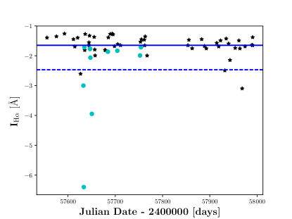
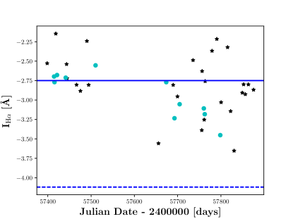
Figure 1: Time series of the H$\alpha$ index I_Hα for the stars EV Lac (top) and YZ CMi (bottom) as black asterisks. Spectra with detected asymmetries are marked by cyan circles. The solid (blue) line marks the median index and the dashed line marks our flare threshold.

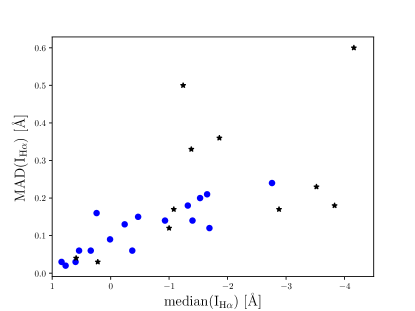
Figure 2: Variability (MAD) of I_Hα as a function of its median value for spectral type M0.0 – M4.0 (blue circles) and M5.0 and later (black asterisks).

In Table 2 we provide the minimum and maximum of the measured I_Hα, as well as its median and median absolute deviation (MAD) for all our sample stars. While for the stars EV Lac and YZ CMi the spread in I_Hα during quiescence as measured by MAD is about the same ($\approx 0.22$ Å; cf. Table 2), the sample stars show a considerable range with DS Leo and CN Leo marking the lower and upper bounds with MADs of $0.02$ Å and $0.6$ Å.

Both the median(I_Hα) and its dispersion as measured by the MAD describe the stellar activity level, and we compare both values in Fig. 2. A correlation seems to be present, indicating lower variability levels for less active stars. This is consistent with the results reported by Bell et al. (2012) and Gizis et al. (2002), who also found larger scatter for more active stars. For our sample, Fig. 2 suggests a flattening of the variability distribution for higher activity levels, which was found neither by Bell et al. (2012) nor Gizis et al. (2002). We therefore consider this to be a spurious result, attributable to the low number statistics for high-activity stars in our sample or to the underestimation of I_Hα for broadened profiles in the stars with the highest activity level.

5 Line wing asymmetries

5.1 Overview

In our M dwarf CARMENES spectra we find diverse examples of H$\alpha$ lines with broad line wings with both relatively symmetric or highly asymmetric profiles. An example of a symmetric profile is given in Fig. 3, which shows four out of the 17 spectra of OT Ser considered in this study. In particular, we show two spectra representing the typical quiescent state of OT Ser (in black), while the spectra plotted in red and cyan represent a more active state. As is shown in Fig. 3, the states are nearly identical in the line core, yet the cyan spectrum exhibits rather broad line wings, reaching about 4 Å beyond the emission core.

To quantify the profile and its asymmetry, we follow Fuhrmeister et al. (2008), Flores Soriano & Strassmeier (2017), and other studies and first obtain a residual spectrum by subtracting the spectrum with the highest (i.e. least active) I_Hα. By subtraction of the spectrum representing the quiescent state, we infer the additional (potentially flaring) flux density and how it is distributed between the narrow line core and the broad line component. We then fit the residual flux density with a narrow and a broad Gaussian profile, representing the line core and wing. The fit with this two-component model results in a reasonably good description of the line profile even in the most asymmetric cases. We nevertheless caution that the fit may be not unique. For example this may happen when one Gaussian flank of the broad component is hidden in the narrow component (see the example in the next section and Fig. 5).

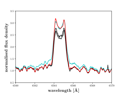
Figure 3: Four normalised H$\alpha$ line profiles of OT Ser. The two black spectra represent the quiescent state of the star, while the red and the cyan spectrum correspond to an enhanced level of activity.

5.2 Red and blue line asymmetries: CN Leo and vB 8

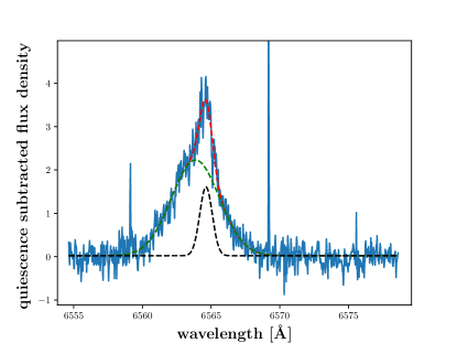
Figure 49: Strongest blue asymmetry was found for vB 8 corresponding to asymmetry no. 44 in Table The CARMENES search for exoplanets around M dwarfs.

A rather striking example of line asymmetries can be found in the CARMENES spectra of vB 8 shown in Fig. 4 (and with two-Gaussian fit in Fig. 49). Three example spectra show the typical variation during the quiescent state. One spectrum shows an extreme blue line asymmetry with only marginal emission in the line core. Two more example spectra both exhibit nearly identical line cores with large amplitudes, but only one of them shows an additional red asymmetry. This demonstrates the variety of profiles encountered in our analysis.

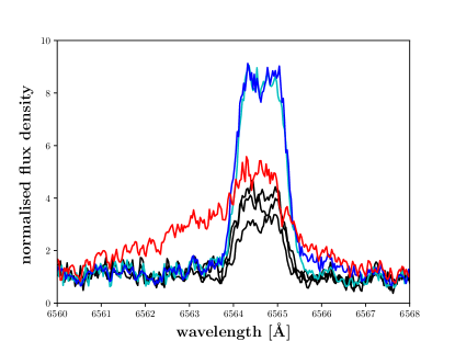
Figure 4: Normalised H$\alpha$ line profiles spectra of vB 8. The three black spectra are typical for the quiescent state, while the red, blue, and cyan spectra show profiles corresponding to enhanced activity levels.

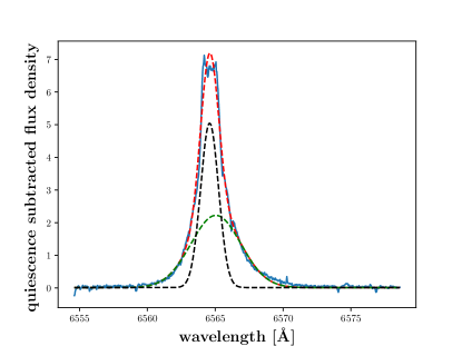
Figure 47: Strongest red asymmetry was found for EV Lac corresponding to asymmetry no. 55 in Table The CARMENES search for exoplanets around M dwarfs.

To illustrate our fits of red and blue line asymmetries, we consider the case of CN Leo. In Fig. 5 we plot the residual H$\alpha$ line profile (i.e. the profile after subtraction of the quiescent state) with a rather moderate red asymmetry along with a two-component fit; in this case we require both the Gaussian component representing the line core and the one representing the wing to be rather narrow. The profile of the emission line core is not entirely Gaussian, especially at the top. Nonetheless, we consider the resulting characterisation of the width and area of the line core sufficiently accurate for our purposes. The problem of the non-uniqueness of the fit is apparent: the width of the wing component cannot tightly be constrained because the blue flank of this component is hidden in the core component. Fortunately, this problem occurs only rarely and the parameters derived for most of the broad components are trustworthy. To further illustrate the quality of our fits, we show the strongest and weakest asymmetry with its corresponding fit for blue and red asymmetries and for more symmetric profiles in Appendix D in Figs. 47 to 52.

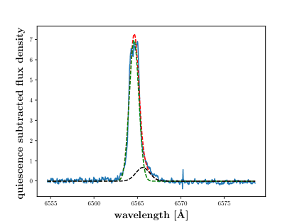
Figure 5: Residual H$\alpha$ line profile of CN Leo (blue) along with best-fit model with two Gaussian components. The dashed red line represents the best-fit two-component Gaussian model, and the dashed black and green lines represent the individual Gaussian components.

5.3 CARMENES sample of broad and asymmetric H$\alpha$ line profiles

In the fashion described above we analysed all H$\alpha$ line profiles. In Table The CARMENES search for exoplanets around M dwarfs we list all detected asymmetries for all sample stars, number them for reference, and provide the best-fit parameters for each of the two Gaussian components: the area in Å, the shift of the central wavelength with respect to the nominal wavelength of the H$\alpha$ line $v_{\rm central}$, and the standard deviation $\sigma$ in Å. Moreover, we list the full width at half maximum (FWHM), the ratio of the Gaussian area $A$ determined for the broad and total components, the epoch of each observation as Julian Date-2 400 000 in days, and the exposure time in seconds. In Appendix A we show all H$\alpha$ line profiles with detected asymmetries, and in Table 2 we summarise statistical aspects of our findings. Specifically, we give the number of detected flares and broad components (categorised into red, blue, and symmetric) and how often both coincide.

6 Discussion

6.1 Overview: statistics

In the 473 CARMENES spectra selected for our study we find a total of 41 flares and 67 line wing asymmetries. Only in eight out of the 28 sample stars, we do not find any H$\alpha$ line observations with broad wings. This indicates a mean duty cycle of $9$ % and $15$ % for flares (following our definition) and H$\alpha$ line asymmetries averaged over the studied sample, respectively. Therefore, broad and asymmetric H$\alpha$ line profiles appear to be a rather common phenomenon among active M stars. Also, line asymmetries are not necessarily linked to flares; in fact, we observe flares without line asymmetries and line asymmetries without flares. Red asymmetries occur more often than blue asymmetries, and symmetric broadening is detected least frequently.

6.2 Limits of the line-profile analysis

The CARMENES observations provide a comprehensive and temporally unbiased sample of M dwarf line profiles, the nature of which imposes, however, some limitations on the analysis. As we lack continuous spectral time series, the course of spectral evolution cannot be resolved, and because integration times vary between less than $100$ s and up to $1800$ s for the faintest objects, variability on short timescales remains elusive. In the specific case of flares, we remain ignorant of the phase covered by the spectrum. Nonetheless, the spectra allow both a statistical evaluation of the sample properties and meaningful analyses of individual profiles. In particular, any sufficiently strong or long-lived structure will be preserved in the individual spectra.

6.3 Physical scenario for line broadening with potential asymmetry

6.3.1 Symmetrically broadened lines

Symmetric line broadening can be caused by the Stark effect or non-thermal turbulence. For the Sun, Švestka (1972) argued that symmetric Balmer line broadening is caused by Stark broadening and not Doppler broadening. More recently, Kowalski et al. (2017b) introduced a new method to handle the Balmer line broadening caused by the elevated charge density during flares to better reconcile modelling and observations.

Another explanation for the more symmetric lines is the long exposure time, possibly blurring phases with blue and red shifts into relatively symmetric, broad lines. Indeed, we see a tendency for broader lines to be more symmetric in our data, but that may be caused by Stark broadening as well (see Sect. 6.9).

6.3.2 Red line asymmetries

As to line asymmetries, Lacatus et al. (2017) presented solar Mg ii h and k line profiles with a striking red asymmetry, observed with the Interface Region Imaging Spectrograph (IRIS) following an X2.1-class flare; the relevant data and fits are shown in their Fig. 2. The authors ascribed the observed line profiles to coronal rain, which is cool plasma condensations travelling down magnetic field lines from a few Mm above the solar surface.

This coronal rain is thought to result from catastrophic cooling and is not only observed in the context of flares, but appears to be a rather ubiquitous coronal phenomenon (Antolin & Rouppe van der Voort, 2012; Antolin et al., 2015). In fact, Antolin & Rouppe van der Voort (2012) supposed that coronal rain is an important mechanism in the balance of chromospheric and coronal material and estimated the fraction of the solar corona with coronal rain to be between $10$ % and $40$ %.

Based on the Mg ii line profiles, Lacatus et al. (2017) derived a net red shift of $60$ km s^-1, which they attributed to bulk rain motion. Velocities on the order of $100$ km s^-1 are, indeed, rather typical for such condensations (e.g. Schrijver, 2001; de Groof et al., 2005; Antolin & Rouppe van der Voort, 2012; Verwichte et al., 2017), which is also the maximum shift we observed.

Along with the red shift, Lacatus et al. (2017) observed broad wings with a Doppler width of $\approx 100$ km s^-1, appearing about six minutes after the impulsive flare phase. Their lines are far broader than the net red shift, which is also true for the majority of our measurements. The authors argue that these widths are best explained by unresolved Alfvénic fluctuations. Broadening by Alfvénic wave turbulence was first suggested by Matthews et al. (2015), based on observations of a solar flare associated with a Sun-quake in the Mg ii h & k lines (see also Judge et al. (2014)).

In a study of spatially resolved H$\alpha$ emission during a solar flare, Johns-Krull et al. (1997) found quiescence subtracted spectra exhibiting weak asymmetries with slightly more flux in the red wing. We completely lack spatial resolution, and the amount of asymmetry reported by Johns-Krull et al. (1997) is so small that we would most likely not have detected it in our spectra. Johns-Krull et al. (1997) interpreted the red wing asymmetry as being caused by rising material absorbing at the blue side of the line.

Besides coronal rain, also chromospheric condensations produce red asymmetries on the Sun. Such condensations normally occur during the impulsive phases of flares driven by non-thermal downward electron beams (e. g. Ichimoto & Kurokawa, 1984; Canfield et al., 1990). These so-called red streaks reach velocities between 40 to 100 km s^-1 with the velocities decreasing on short timescales and the emission ceasing before H$\alpha$ emission reaches its maximum. Canfield et al. (1990) measured only velocities up to 60 km s^-1 and ascribed this low maximum velocity to their comparably low time resolution of 15 s. Also Graham & Cauzzi (2015) found lower velocities and very short decay times of only about one minute, which even partially preceded the also observed up-flows.

For the Si iv and C ii transition region lines, Reep et al. (2016) found red emission asymmetries lasting more than 30 min and attributed these to the successive energisation of multiple threads in an arcade-like structure. The authors argue against coronal rain because no blue shifts were detected at the beginning of the flare. Instead, the red shifts started simultaneously with a hard X-ray burst. Reep et al. (2016) further argue that a loop needs some time to destabilise for coronal rain to start after the heating ceases. Rubio da Costa et al. (2016) and Rubio da Costa & Kleint (2017) modelled solar flare observations in H$\alpha$, Ca ii 8542 Å, and Mg ii h & k with multi-threaded down-flows but still had trouble reproducing the observed wing flux in their models.

Since we lack information about when during the flare the emission responsible for the broad components occurred (and if at all in some cases), we cannot properly distinguish between the coronal rain and chromospheric condensation scenario. While coronal rain is expected to take place later in the decay phase, chromospheric condensations are thought to be associated with the impulsive phase. We consider it improbable though that transient events lasting only about a minute can account for the strongest asymmetric signatures in our up to 30-minutes-long exposures. Moreover, the blue asymmetries found in our sample are never associated with large amplitudes in the narrow main component, suggesting coverage of the flare onset only (as expected; see Sect. 6.3.3 and 6.3.1). In contrast, elevated emission in the narrow component was detected for some lines with red asymmetries, which indicates that at least the onset of the decay phase was covered; however, the impulsive phase may be covered, too. While it appears to us that the coronal rain scenario is more easily compatible with the majority of our observations, we cannot ultimately discriminate between the scenarios on the basis of our data, and both phenomena may actually have occurred.

6.3.3 Blue line asymmetries

On the Sun, blue asymmetries are also observed. For instance, Cho et al. (2016) reported the appearance of a blue asymmetry in the H$\alpha$ line associated with the start of a rising filament preceding a solar flare. The authors attribute the asymmetry to a mixture of material moving at velocities between $-138$ km s^-1 and $38$ km s^-1. While Cho et al. (2016) reported an excess absorption in H$\alpha$, blue shifted emission has also been observed on the Sun (Švestka et al., 1962; Tang, 1983). In fact, the flare observations of the mid-M dwarfs CN Leo and Proxima Centauri, which also cover the flare onset, show both blue asymmetries during flare onset, followed by red asymmetries later on during the decay phase (Fuhrmeister et al., 2008, 2011). Accordingly, we ascribe the blue shifted components to chromospheric evaporation.

6.4 Strength of the asymmetries

As a way to measure the strength of the asymmetry, we compute the area of the broad Gaussian multiplied by the shift of its central wavelength. We show this asymmetry strength in Fig. 6.

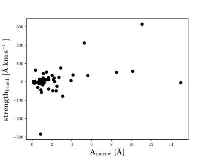
Figure 6: Strength of the asymmetries as a function of the narrow component amplitude.

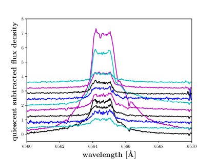
Figure 33: Spectra with asymmetry for EV Lac; from bottom to top the spectra correspond to entry nos. 54 – 64 in Table The CARMENES search for exoplanets around M dwarfs.

Based on this measure, we find three outstandingly strong asymmetries. The one with the blue shift belongs to vB 8 and the corresponding spectrum is shown in Fig. 4. The remaining two correspond to asymmetries no. 50 and 55 in Table The CARMENES search for exoplanets around M dwarfs, are red shifted, and stem from EV Lac. The associated spectra are shown in Fig. 33 (and with Gaussian fit in Fig. 47). The first of these asymmetries (no. 50) also shows the second highest flux level in the narrow line along with broad wings in the Na i D lines. It is clearly associated with a large flare on EV Lac.

6.5 Connection of asymmetries to flares

As evidenced in Table 2, broad wings in H$\alpha$ with more or less pronounced asymmetries of the broad component appear to be quite common among M stars. In contrast to the literature, where wings and asymmetries therein are normally connected to flares, many asymmetries found in our study do not coincide with flares (using our flare definition). Assuming that stellar flares show a sufficiently uniform pattern of chromospheric line evolution, this finding shows that: (i) line asymmetries may not in all cases be connected to flares; (ii) they may be found also in smaller flares, (iii) they may persist up to or even beyond the end of the decay phase of stronger flares, or, (iv) they occur during the impulsive phase, where the chromospheric lines just start to react to the flare. We cannot distinguish these latter three scenarios since we do not have time series, but only snapshots. The last possibility is rather unlikely, since the impulsive phase of flares typically lasts only a few tens of seconds, while the typical exposure times of our sample stars is a few hundred seconds, so that in most cases also the flare peak should be covered by the exposure.

Despite the lack of a clear association between asymmetries and flares, asymmetries generally seem to be accompanied by somewhat enhanced activity states: only in six cases, where an asymmetry was detected, did the narrow Gaussian component area remain small (¡0.5 Å), indicating that the stellar activity state was only marginally higher than the minimum state that we subtracted. In all other cases, we found indications for enhanced emission in the narrow component, albeit not sufficiently strong to be qualified as a flare.

Moreover, we find that the pEW(H$\alpha$) of the broad component increases as the strength of the narrow component of the H$\alpha$ line increases (see Fig. 7). A similar correlation between the stellar activity state and the strength of the broad component was found by Montes et al. (1998). Formally, we obtain a Pearson correlation coefficient of 0.43, taking all spectra into account where we found a broad component. Excluding the four values pertaining to CN Leo and vB 8 (see Fig. 7), we compute a correlation coefficient of 0.88. CN Leo and vB 8 are the only two stars in the sample with spectral type M6 or later for which we found asymmetries, but we are not aware of any physical reason why these two stars should behave differently, though they may have higher contrast to photospheric emission in this wavelength region.

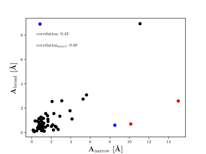
Figure 7: H$\alpha$ line residual pEW(H$\alpha$) in the broad component versus the narrow residual pEW(H$\alpha$) both measured by the Gaussian area, A, of the line fit. Red dots correspond to the two values for CN Leo and blue dots to the two values for vB 8. Correlation coefficients correspond to the whole sample and the sample excluding CN Leo and vB 8.

6.6 Occurrence rate of asymmetries and activity state or spectral type

According to our analysis the four fastest rotators in our sample (V374 Peg, LSR J1835+3259, StKM 2-809, and GL Vir) with $v\sin i$ ranging from 21 km s^-1 to 43 km s^-1 all show asymmetries. For the fastest rotator, V374 Peg, a member of the roughly 300 Myr old Castor moving group (Caballero (2010), but see Mamajek et al. (2013)), we also detect the highest fraction of asymmetries. On the other end of the activity range, we find that three out of the eight stars without any detected asymmetry are less active, showing weak H$\alpha$ emission (DS Leo, HH And, and BD–02 2198). Both hint at a relation between activity state and the frequency of asymmetries.

In Fig. 8 we show the fraction of spectra exhibiting asymmetries as a function of (projected) rotational velocity (top) and median(I_Hα) (bottom). With a mean fraction of 5 %, the probability of showing an asymmetry is smaller for slowly rotating stars ($<3.5$ km s^-1) than for fast rotators, where the mean fraction is 23 %. A t-test shows a probability of about 1 % that the two means are equal.

The picture is similar for the rate of asymmetries as a function of the median(I_Hα) (Fig. 8, bottom panel). We find the highest fractions of asymmetric line profiles among the more active stars. In fact, the distribution suggests the existence of an upper envelope indicated by the dashed line in Fig. 8. While we cannot determine any formal justification, the presence of an upper envelope appears to be plausible, if the asymmetries are related to the release of magnetic energy into the stellar atmosphere. At lower activity levels such releases would then be expected to occur less frequently than at higher activity levels, where they can – but apparently do not need to – lead to detectable line profile asymmetries.

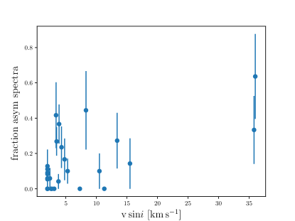
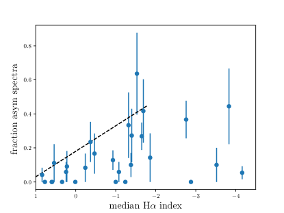
Figure 8: Fraction of spectra with asymmetries (blue circles) as a function of rotational velocity (top) and median(I_Hα) (bottom) with a tentative upper envelope (dashed black line).

Another parameter that may relate to the occurrence of asymmetries is spectral type. We plot the distribution of the fraction of asymmetries as a function of spectral type in Fig. 9. There seems to be a concentration of a high occurrence rate of asymmetries around the mid-M spectral types. The mean occurrence rate for early spectral types (M0 – M2.5 V) is 0.07, while for mid spectral type (M3 – M5.0 V) it is 0.17, and for even later spectral types it is 0.14. We caution though, that this may be caused by selection effects, since for example all our early stars are slow rotators.

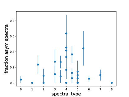
Figure 9: Fraction of spectra with asymmetries (blue circles) as a function of spectral type.

Table 2: Statistics of detected asymmetries and I_Hα measurements.

Star	Archived	Used	$N_{\rm flare}$	$N_{\rm asymmred}$	$N_{\rm asymmblue}$	$N_{\rm symm}$	$N_{\rm flare,asymm}$	IHα
								max	min	median	MAD
V388 Cas	11	10	0	1	0	0	0	-2.93	-5.06	-3.52	0.23
YZ Cet	17	17	4	1	0	0	1	0.48	-0.90	0.24	0.16
LP 768-113	10	10	5	0	0	0	0	0.17	-0.23	0.01	0.09
Barta 161 12	11	(11)	(1)	(1)	(3)	(1)	(0)	-0.93	-2.05	-1.32	0.34
TZ Ari	14	12	4	0	1	0	1	-0.08	-0.57	-0.24	0.13
GJ 166 C	49	39	1	2	1	2	0	-0.65	-1.53	-0.93	0.14
V2689 Ori	25	24	0	1	0	0	0	0.89	0.75	0.84	0.03
G099-049	13	12	2	1	0	1	1	-0.24	-0.79	-0.47	0.15
BD-022198	11	8	1	0	0	0	-	0.65	0.37	0.60	0.03
YZ CMi	32	29	0	5	4	2	0	-2.14	-4.41	-2.76	0.24
GJ 362	10	9	0	0	0	1	0	0.63	0.47	0.54	0.06
CN Leo	43	37	3	1	0	1	2	-2.17	-10.60	-4.16	0.60
DS Leo	27	26	0	0	0	0	0	0.81	0.70	0.77	0.02
WX UMa	12	9	0	1	2	1	0	-2.83	-4.05	-3.83	0.18
StKM 2-809	11	9	0	1	1	1	0	-0.98	-1.73	-1.32	0.18
GL Vir	10	7	0	1	0	0	0	-1.28	-2.25	-1.86	0.36
OT Ser	17	17	2	1	2	1	2	-0.23	-0.64	-0.37	0.06
G180-060	11	6	0	0	0	0	0	-2.52	-3.22	-2.88	0.17
vB 8	64	20	5	1	1	0	2	-0.32	-4.62	-1.38	0.33
LP 071-082	12	11	1	0	0	0	-	-0.87	-1.67	-1.00	0.12
J18174+483	11	11	0	0	1	0	0	0.34	0.18	0.22	0.03
Ross 149	11	11	2	0	0	0	-	0.42	-0.01	0.34	0.06
G141-036	19	17	1	1	0	0	1	-0.65	-3.57	-1.08	0.17
vB 10	22	16	0	0	0	0	-	0.83	-3.96	-1.24	0.50
V374 Peg	12	11	1	3	2	2	1	-1.14	-2.93	-1.53	0.20
EV Lac	45	41	4	6	3	2	3	-1.26	-6.40	-1.65	0.21
GT Peg	12	12	1	2	0	1	1	-1.04	-2.50	-1.40	0.14
HH And	30	30	3	0	0	0	0	0.74	0.01	0.59	0.04
RX J2354.8+3831	13	12	1	3	2	0	1	-1.31	-2.67	-1.69	0.12
Total		473	41	32	20	15	16

Note: The spectra of Barta 161 12 are not counted in the total.

6.7 The narrow Gaussian component

The mean width of the narrow Gaussian component as measured by its FWHM found in our analysis is $65$ km s^-1 with a standard deviation of $10$ km s^-1. The mean absolute shift of the narrow Gaussian core components is $3.9$ km s^-1, which is significantly lower than its mean width and about an order of magnitude less than the mean absolute shift of $35$ km s^-1 found for the broad component. For only nine spectra we measure a shift exceeding 10 km s^-1. Of these, five originate from the fast rotator V374 Peg, for which we suspect a rotational contribution to the shift (see also Sect. 6.10). The four remaining cases are due to TZ Ari, OT Ser, vB 8, and WX UMa, where the shift cannot be explained by rotation. In the specific case of OT Ser, the spectrum also appears to suffer from some spectral defects that may influence the fit.

We find only small shifts in the position of the core component of the H$\alpha$ line as measured by the narrow Gaussian component, in particular when compared with the line width. The shift in the position of the narrow Gaussian component is uncorrelated with its area. The distribution is shown in Fig. 10. At any rate, the two-component Gaussian model only provides an approximate representation of the true line profile, which is generally more complex, so that some residual shifts are expected. The scatter appears to decrease for stronger emission line cores, which may be due to a better constrained fit in these cases. Therefore, we consider the measurements consistent with a stationary emission line core.

6.8 Shift of the broad Gaussian component

The measured shift of the broad component varies between about $-100$ and $100$ km s^-1. There are 15 (22 %) spectra showing a shift of less than $\pm 10$ km s^-1 in the broad component. In analogy with the distribution of shifts in the narrow component (see Sect. 6.7), we consider these shifts insignificant and the profiles symmetric. In our sample, we also find a surplus of red shifted broad wings. Only considering broad components with an absolute shift larger than $10$ km s^-1, we find 20 blue shifted ($30$ %) and 32 red shifted ($48$ %) components, while for absolute shifts larger than 50 km s^-1, there are four (6 %) blue shifted and 13 (19 %) red shifted components. An excess of red asymmetries is also consistent with observations of solar flares (Švestka et al., 1962; Tang, 1983).

In the context of our envisaged scenario, the asymmetric line profiles do require atmospheric motions. We note that all measured velocities are far below the escape velocity of 500 to 600 km s^-1 for mid to early M dwarfs. Theoretically, a (radial) mass ejection at the limb would be observed at much lower velocity due to projection effects, but we consider improbable the possibility of observing ejections only at the stellar limb and not at the centre. Assuming a strictly radial motion and a true velocity of $500$ km s^-1, only $20$ % of all directions yield projected velocities of $\pm 100$ km s^-1 or less. Thus, we consider it unlikely that the observed blue shifts are exclusively due to limb ejections, although we cannot rule out the possibility in individual cases. However, even the extreme case of a blue asymmetry in vB 8 (Fig. 4) does not require any material near the escape velocity because the largest shifts in the line flank at about 6561 Å correspond to velocities of only 160 km s^-1.

Turning now to red shifts, the observed red shifts are comparable with the speeds measured for solar coronal rain, and we consider a phenomenon similar to coronal rain a viable explanation for the observed line shifts. An alternative explanation could be chromospheric condensations.

In the context of our scenario (see Sect. 6.3), blue asymmetries would be associated with rising material, primarily in the early phases of flares. In Fig. 10 we show the shift of the broad component as a function of continuum-normalised flux, which shows a striking absence of blue shifts for fluxes in the narrow component higher than about 3 Å. A single exception corresponds to a spectrum of CN Leo, showing a rather marginal blue shift (which anyway makes it a symmetric case). For weaker narrow components, the distribution is more balanced. We argue that spectra showing strong blue shifted asymmetries with weak narrow components cover primarily the onset of a flare, where the line cores do not yet show a strong response. The case of CN Leo may be explained by the exposure covering both the flare onset, peak, and potentially a fraction of the decay phase. Then, both blue and red asymmetries would mix and give the appearance of a broad line with only marginal net shift and substantial flux in the narrow component.

While the observed shifts can, therefore, be reconciled with our scenario, red and blue shifts are caused by completely different physical processes. In light of this, it appears remarkable that the maximum velocities of the observed blue and red shifts are so similar and we currently lack a concise physical explanation for this.

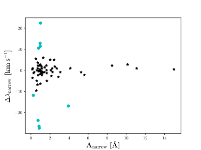
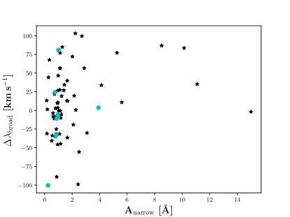
Figure 10: Shift of narrow (left panel) and broad (right panel) Gaussian component as a function of their continuum-normalised residual flux density (measured by the Gaussian area A of the residual line fit). Cyan dots mark outliers showing absolute shifts exceeding $10$ km s^-1 in the narrow component.

6.9 Width of the broad component

The fitted widths of the broad component vary between 0.5 and 3.6 Å with a mean of 1.72 Å, corresponding to a velocity of $184.9$ km s^-1 as FWHM. In Fig. 11 we show the distribution of the width of the broad and narrow Gaussian components as a function of their shift; the numbers are given in Table The CARMENES search for exoplanets around M dwarfs. Typical values range between $100$ and $200$ km s^-1 with a maximum of $390$ km s^-1. Visual inspection of the fits shows, however, that the top two widths of $390$ and $365$ km s^-1, corresponding to flares on EV Lac and GT Peg, are probably overestimated.

The distribution shown in Fig. 11 suggests a decrease in the width as the shift increases either to the red or the blue side. This impression is corroborated by a value of $-0.54$ for Pearson’s correlation coefficient between the width and the absolute value of the shift (excluding the two outliers); the p-value for a chance result is $3\times 10^{-6}$. A stronger contribution of Stark broadening at smaller shifts is conceivable. Also the coarse time resolution may play a role, because most exposures that cover the short flare onset should also cover the flare peak and the start of the decay phase. In our sample, we do not find strong blue asymmetries in combination with strong narrow components. We argue that this indicates that evaporation was accompanied by red asymmetries in all cases studied here. This could indicate that evaporated material increases the density in the coronal loops, leading to more efficient cooling, followed by H$\alpha$ rain. A red coronal rain asymmetry from the flare peak then adds to the broadening, making the profile more symmetric.

When the shift of the broad component is sufficiently small for the H$\alpha$ line to be considered symmetric, we cannot distinguish if the lines are broadened by high charge density, turbulence, or downward and upward moving material, whose distinct signatures are smeared out due to the long integration time. In fact, the latter effect may account for widths in excess of $300$ km s^-1, which appear high for an interpretation in terms of turbulence. However, the majority of the broadened lines show substantial asymmetry in the broad component for which Stark broadening does not appear to be a viable explanation. In their modelling of a chromospheric condensation computed to represent a solar flare event, Kowalski et al. (2017a) find that Stark broadening does play a significant role for the Balmer lines but not for other lines. The authors find red asymmetries with the line width from instantaneous model snapshots to be actually lower than that observed. The inclusion of moderate micro-turbulence, together with the velocity evolution of the shifts in the model accumulated over the exposure time, leads to a realistic broadening in their study. The determined widths of the broad component are comparable to those observed in the Mg ii lines by Lacatus et al. (2017) on the Sun. By analogy, we consider magnetic turbulence a viable broadening mechanism to explain the observed widths of the H$\alpha$ lines.

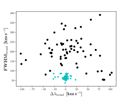
Figure 11: Width of the broad (black) and narrow (cyan) components as a function of their shift.

6.10 H$\alpha$ line profiles of the fast rotators Barta 161 12, StKM 2-809, and V374 Peg

The three fastest rotators Barta 161 12, StKM 2-809, and V374 Peg show complex features in the H$\alpha$ line profiles observed by CARMENES. For all three stars the H$\alpha$ line profile continuously varies. In Fig. 12 we show three H$\alpha$ line profiles (prior to subtraction) of StKM 2-809, namely, those with the weakest and strongest detected H$\alpha$ lines and a spectrum with intermediate line strength. The lowest-activity H$\alpha$ line profile shows a more pronounced blue wing than the intermediate-activity spectrum shown here. Subtracting the lowest-activity state spectrum produces relative absorption features in the residual spectrum in the blue flank of the H$\alpha$ line. For StKM 2-809, we find such features in two out of three spectra with asymmetry, but some spectra without marked asymmetry show also complex H$\alpha$ line profiles. In this case, the absorption features may influence our fits but not to a degree that would call the presence of additional shifted emission into question. Therefore, we include the star in our normal analysis since we believe that the main effect is similar to that in slower rotators.

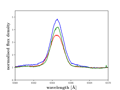
Figure 12: Normalised strongest (blue), weakest (red), and medium-activity (green) H$\alpha$ line profiles of StKM 2-809 observed by CARMENES.

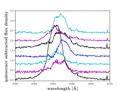
Figure 32: Spectra with asymmetry for V374 Peg; from bottom to top the spectra correspond to entry nos. 47 – 53 in Table The CARMENES search for exoplanets around M dwarfs.

For V374 Peg only one spectrum shows a significant relative absorption feature along with an asymmetry (see Fig. 32, fourth from bottom). Therefore, we believe that also for V374 Peg the asymmetries are mainly caused by the same mechanism, although some profiles also show plateaus and one profile is double-peaked (second from bottom in Fig. 32).

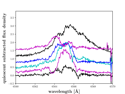
Figure 17: Spectra with asymmetries for Barta 161 12; from bottom to top the spectra correspond to entry nos. 3 – 7 in Table The CARMENES search for exoplanets around M dwarfs. The second spectrum from the top (black line) is shown in addition to the data in Table The CARMENES search for exoplanets around M dwarfs because it exhibits significant asymmetry but it could not be fitted satisfactorily with two Gaussians.

Barta 161 12 shows the most pronounced variety of H$\alpha$ profiles, which in many cases need more than two Gaussians for fitting (Fig. 17) representing a different case of asymmetries. Only one spectrum of this star seems to fall into the category of asymmetries discussed in this paper. Therefore, we exclude it from our analysis as already mentioned in Sect. 3. For the other two fast rotators the situation is less extreme. All three stars show significant shift in the narrow H$\alpha$ line component but never higher than their rotational velocity.

Whether or not the relative absorption features seen in the subtracted spectra of the three fast rotators are due to true absorption, for example caused by a prominence, or are the results of excess emission in the lowest-activity spectrum used in the subtraction cannot be determined on the basis of our data. We also want to note the possibility that the plateaus and multi-peaked spectra of especially Barta 161 12 (Fig. 17, top two spectra) may originate in distinct active regions, rotating along with the stellar surface.

6.11 Broad components and asymmetries in other lines

6.11.1 The optical Na i D and He i D₃ lines

The optical arm of CARMENES covers further known activity indicators beyond the H$\alpha$ line. In particular, we investigated the Na i D and He i D₃ lines and, indeed, found asymmetric components in a number of spectra of EV Lac, OT Ser, and StKM 2-809.

In Fig. 13 we show an example for the star OT Ser; the corresponding H$\alpha$ line profiles are presented in Fig. 3 with the same colour coding. While two enhanced spectra in the H$\alpha$ line are nearly identical, this is not true for the corresponding He i D₃ and Na i D lines, indicating a different state of the chromosphere at the two times.

Because the broad components of the two Na i D lines overlap, we fit them simultaneously with a total of four Gaussian components, representing two narrow and two broad components. We fix the offset in wavelength of the narrow and broad components to the known doublet separation and also couple their respective widths. The best-fit values for the three spectra with broad wings in Na i D and He i D₃ are given in Table 3; the spectra are also indicated in the notes column of Table The CARMENES search for exoplanets around M dwarfs.

The narrow Gaussian component is in all cases only slightly shifted, and its width stays about the same, with the He i D₃ line being slightly broader than the Na i D lines. Both lines are significantly narrower than the narrow component of the H$\alpha$ line, which is broader because it is optically thick for our sample stars. For the broad component, the picture is more complicated with most of the fit results for the individual lines – also compared to the broad component of the H$\alpha$ line – differing significantly.

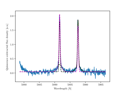
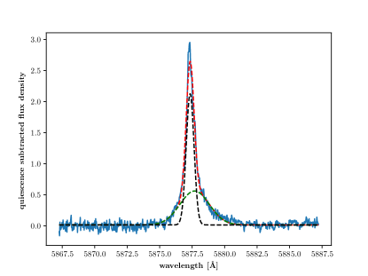
Figure 37: Spectrum with asymmetry for EV Lac.

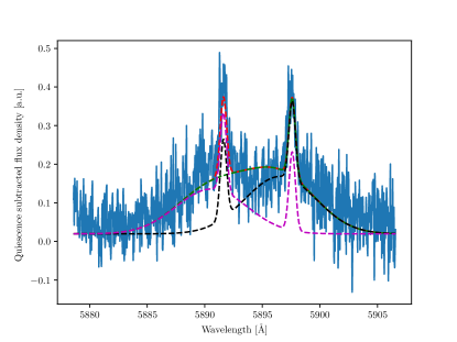
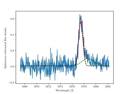
Figure 38: Spectrum with asymmetry for StKM2-809.

These differences may be caused by the different height at which the lines originate in the atmosphere; H$\alpha$ is thought to be formed in the upper chromosphere, while the Na i D lines originate in the lower chromosphere. Although we consider the fits satisfactory (see Figs. 36–38), part of the differences may also be attributable to problems in the fit itself such as the approximation by Gaussian profiles. However, Figs. 36–38 demonstrate that the He i D₃ line shows a red asymmetry in StKM 2-809, while the Na i D lines are more symmetric, exhibiting emission in the blue wing as well. Thus we are confident that a physical reason underlies the line profile differences, which may be related to distinct sites of line formation and radiative transfer. Again, however, we caution that the phenomena may actually not have occurred simultaneously, but arise from time averaging during the exposure (see Sect. 6.2).

The spectrum of OT Ser showing broadening in the Na i D lines also exhibits relatively symmetric, broad wings in the H$\alpha$ line. While the latter may be caused by Stark broadening, the Na i D lines are not thought to be affected by this. Therefore, the broadened Na i D lines suggest a different broadening mechanism, probably turbulence, at least in this individual case.

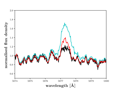
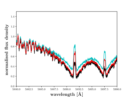
Figure 13: Line asymmetries in spectra of OT Ser. Normalised He i D₃ (top) and Na i D line profiles (bottom). In both cases, we show two typical quiescent spectra in black along with two spectra of enhanced activity in cyan and red (same spectra and colour coding as in Fig. 3).

Table 3: Detected asymmetries in Na i D (5891.58 and 5897.56 Å) and He i D₃ (5877.24 Å).

Star	Line	Gauss 1					Gauss 2
		Area	$\lambda_{\rm{central}}$	$v_{\rm{central}}$	$\sigma$	FWHM	Area	$\lambda_{\rm{central}}$	$v_{\rm{central}}$	$\sigma$	FWHM
			[Å]	[km s-1]	[Å]	[km s-1]		[Å]	[km s-1]	[Å]	[km s-1]
OT Ser	Na i D1	0.12	5897.54	$-1.0$	0.20	24.0	0.27	5897.64	4.1	1.97	236.
OT Ser	Na i D2	0.13	5891.56	$-1.0$	0.20	24.0	0.34	5891.66	4.1	1.97	236.
OT Ser	He i D3	0.37	5877.37	6.6	0.34	40.8	0.35	5878.47	62.7	2.74	329.0
EV Lac	Na i D1	0.70	5897.59	1.5	0.17	20.4	0.29	5897.59	1.5	0.80	95.8
EV Lac	Na i D2	0.72	5891.61	1.5	0.17	20.4	0.51	5891.61	1.5	0.80	95.8
EV Lac	He i D3	1.60	5877.34	5.1	0.30	36.0	1.5	5877.6	18.4	1.11	133.3
StKM 2-809	Na i D1	0.19	5897.55	0.	0.40	47.9	0.65	5897.04	$-26.5$	2.44	292.3
StKM 2-809	Na i D2	0.19	5891.58	0.	0.40	47.9	0.79	5891.06	$-26.5$	2.44	292.3
StKM 2-809	He i D3	0.47	5877.45	10.7	0.34	40.8	0.23	5878.49	63.7	0.85	102.1

6.11.2 The He i and Pa$\beta$ near-infrared lines

The infrared arm of CARMENES also covers known chromospherically-sensitive lines such as the Pa$\beta$ line and the He i line at $10833.31$ Å, the latter of which has primarily been used in the solar context (e.g. Andretta et al., 2017). We searched all 72 spectra with asymmetries in H$\alpha$ also for asymmetries in He i 10833 Å and Pa$\beta$. Unfortunately, not all available optical spectra have infrared counterparts (cf., Table The CARMENES search for exoplanets around M dwarfs). For the analysis, 40 spectra were available of which we discarded four because of the telluric contamination was too severe. Of the 36 usable spectra, 19 show no excess in the He i line, two show a weak excess, and 15 a clear excess. Unfortunately, the low excess flux in the Pa$\beta$ lines precludes a meaningful analysis of its symmetry here.

We show the 15 excess spectra in Appendix C in Figs. 39 to 46 along with the corresponding Pa$\beta$ excess fluxes. Also for the He i 10833 Å line, the degree of asymmetry is hard to assess in most cases because the red side of the line is contaminated by strong air glow or telluric lines.

In Fig. 14, we show the He i and Pa$\beta$ lines of EV Lac (the corresponding spectra are also marked by ‘IR’ in Table The CARMENES search for exoplanets around M dwarfs). The infrared regime is more heavily affected by telluric contamination and air glow lines (Rousselot et al., 2000). Because a number of strong lines are located in the direct vicinity of the He i line (cf., Fig. 14), and an appropriate correction is very challenging, we limit ourselves to a qualitative analysis. In Fig. 14, we show four spectra with enhanced emission in the quiescent subtracted flux density. While three spectra do not show clear signs of an asymmetry, one spectrum does exhibit a strong blue asymmetry (taken at JD 2 457 632.6289 d, cf., Table The CARMENES search for exoplanets around M dwarfs) and also the corresponding H$\alpha$ line shows a blue asymmetry in this case. In the Pa$\beta$ line, we find enhancements in the line flux for the three flare spectra as can be seen in the bottom panel of Fig. 14. Like the spectrum described above, this one also suggests a blue asymmetry.

The two infrared lines studied here clearly react to different activity states. In our spectra, emission in the He i 10833 Å line is clearly detected in $34$ % of the available infrared spectra also showing an H$\alpha$ asymmetry, while the Pa$\beta$ line appears to be less sensitive to chromospheric states causing broad wings. Asymmetries are difficult to assess in the Pa$\beta$ and He i 10833 Å line. Only in three cases, namely two spectra of EV Lac (first two) and the last spectrum of StKM 2-809, we are confident that a blue asymmetry is present in the He i 10833 Å line. These correspond also to blue shifts in H$\alpha$.

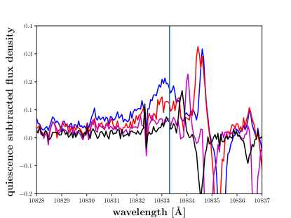
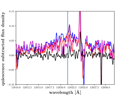
Figure 14: Line asymmetries in infrared spectra of EV Lac. Top: The quiescence subtracted He i 10833 Å  line profile. Bottom: The quiescence subtracted Pa$\beta$ line profiles smoothed over eight bins for reduction of noise. The colours indicate different active spectra of EV Lac but correspond to the same spectra for both lines. In both cases the reference central wavelength is marked by the blue vertical line.

7 Conclusions

We present the most comprehensive high-resolution spectral survey of wings and asymmetries in the profiles of H$\alpha$ and other chromospheric lines in M dwarfs to date. We found 67 asymmetries in 473 spectra of 28 emission-line M dwarf stars. Line wing asymmetries in the H$\alpha$ line, therefore, appear to be a wide-spread phenomenon in active M dwarfs, which we find in about 15 % of the analysed spectra. Only eight stars do not show any wings or asymmetries.

In contrast to that, asymmetries in other spectral lines seem to occur less frequently. In particular, only 4 % of the spectra with detected H$\alpha$ asymmetry show also an asymmetry in the optical Na i D and He i D₃ lines. In the He i 10833 Å line, we find broad wings for 34 % of the cases. Excess emission in the Pa$\beta$ line was found only in a few cases, but we considered a meaningful analysis of its asymmetry unfeasible.

While the occurrence rate of the asymmetries varies widely between stars, we find a relation with the stellar activity level. In particular, more active stars (as measured by rotational velocity or median(I_Hα)) also show a higher fraction of spectra with asymmetric H$\alpha$ line profiles. Nevertheless, we find that only 24 % of the asymmetries are associated with a flare, as defined by our flare criterion, and we conjecture that either asymmetries are not necessarily coupled to (large) flares or they can persist to the very end of the decay phase.

We find our results to be consistent with a scenario in which red asymmetries are associated with coronal rain or chromospheric condensations, two phenomena well known from the Sun. Unfortunately, they cannot be distinguished on the basis of the occurring velocities or line width, and we lack the timing information of when (and sometimes if) during a flare the asymmetry occurs. Lacatus et al. (2017) explain the width by Alfvénic turbulence, which may also cause the broadening in our case. Because of the relatively long exposure times for M dwarfs, however, we cannot rule out that the width is due to an evolution in the velocity field.

For the blue wing enhancements, we propose chromospheric evaporation as the mechanism responsible, which explains why we do not find substantially blue shifted broad components in combination with strong narrow core components. Supposedly, the chromospheric evaporation occurs during the early impulsive stage of a flare, while the largest amplitudes in chromospheric lines are typically observed at flare peak or early decay phase. While also symmetric line profiles may be explained by coronal rain with low (projected) velocities or time average effects, we cannot exclude Stark broadening as an alternative explanation. One exception here is the case of OT Ser, which exhibits a symmetrically broadened H$\alpha$ line along with broadened Na i D lines, which is not expected for the Stark effect; in fact, Stark broadening affects higher Balmer lines more strongly than H$\alpha$ itself. While CARMENES does not cover these lines, a dedicated study of the effect may take advantage of this fact.

While the data presented here are well suited for a statistical study of broadening and asymmetry in the H$\alpha$ line, there is a clear need for further observations. Any detailed modelling attempt would greatly benefit from dedicated observations that clarify whether asymmetries are coupled to flares in all cases and if so, which sort of asymmetry (red or blue) is associated to which phase of the flare. Therefore, to better understand the phenomenon of asymmetric line profiles, continuous spectral time series with a higher temporal cadence (or simultaneous photometry) and spectral coverage of the end of the Balmer series are definitely needed.

Table 4: Detected asymmetries.

no.	Name	Epoch	$t_{\rm exp}$	Gauss 1				Gauss 2				Abroad/	Remarksc
		Julian date		Area	$v_{\rm central}$	$\sigma$	FWHM	Area	$v_{\rm central}$	$\sigma$	FWHM	Atotal
		-2 400 000[d]	[s]	[Å]	[km s-1]	[Å]	[km s-1]	[Å]	[km s-1]	[Å]	[km s-1]
1	V388 Cas	57749.4020	1589	4.13	0.9	0.54	58.1	1.10	33.8	2.06	221.5	0.21	IR
2	YZ Cet	57622.5718	444	2.71	0.9	0.46	49.5	0.24	99.5	0.74	79.6	0.08	tech
3	Barta 161 12	57622.6627	1700	0.86	29.2	0.74	79.6	0.16	-37.4	0.5	53.8	0.16	tech
4		57642.6235	1800	1.72	25.1	0.54	58.1	0.74	-46.1	2.20	236.5	0.30	IR
5		57688.5189	1802	1.87	16.4	0.73	78.5	3.47	98.2	2.97	319.3	0.65	IR
6		57703.4290	1719	2.41	13.7	0.80	86.0	0.35	-90.4	1.00	107.5	0.13	IR
7		57763.3199	1802	0.42	-25.6	0.33	35.5	1.26	-1.4	1.61	173.1	0.75	IR
8	TZ Ari	57766.2898	504	0.87	0.	0.54	58.1	0.32	-11.0	1.51	162.3	0.42
9	GJ 166 C	57634.6243	263	0.97	2.7	0.69	74.2	0.96	10.5	2.11	226.9	0.50	tech
10		57636.6648	277	1.14	0.9	0.55	59.1	0.23	-0.5	1.54	165.6	0.17	tech
11		57705.5112	222	0.93	-0.5	0.58	62.3	0.69	9.6	1.86	200.0	0.43
12		57712.5133	551	1.24	-0.9	0.58	62.3	0.75	19.2	1.93	207.5	0.38
13		57799.3539	492	1.17	-1.4	0.49	52.7	0.52	-10.0	2.26	243.0	0.31
14	V2689 Ori	57414.3922	769	0.28	-1.4	0.50	53.8	0.07	44.3	1.61	173.1	0.2	tech
15	G 099-049	57694.6742	362	0.63	0.	0.54	58.1	0.31	-8.2	1.20	129.0	0.32	tech
16		57699.6356	702	0.96	0.	0.54	58.1	0.41	26.5	1.09	117.2	0.30
17	YZ CMi	57414.5293	1000	0.72	0.9	0.58	62.3	0.84	-11.0	1.61	173.1	0.54	tech
18		57415.4739	1100	1.11	-0.5	0.53	57.0	0.72	27.4	2.27	244.1	0.39	tech
19		57421.3962	650	0.96	-1.8	0.62	66.6	0.65	3.7	2.40	258.0	0.40	tech
20		57441.3985	1000	0.99	-6.3	0.57	61.3	0.26	46.6	0.80	86.0	0.21
21		57510.3330	800	0.57	-9.6	0.80	86.0	0.92	-33.8	1.80	193.5	0.62	tech
22		57673.6632	239	1.08	-1.4	0.56	60.2	0.55	-31.5	1.80	193.5	0.34
23		57692.7212	161	2.23	0.9	0.60	64.5	0.20	103.2	0.84	90.3	0.08
24		57704.5994	267	1.64	0.	0.59	63.4	0.57	39.7	1.88	202.1	0.26
25		57760.4882	262	1.66	-1.4	0.55	59.1	1.08	-36.5	2.02	217.2	0.39
26		57762.6101	234	2.15	-2.7	0.64	68.8	0.62	19.6	2.10	225.7	0.22	tech
27		57798.4688	424	2.27	-0.9	0.59	63.4	1.55	0.5	1.96	210.7	0.41	tech
28	GJ 362	57442.4760	1000	0.20	0.9	0.47	50.5	0.12	1.4	1.55	166.7	0.37	tech
29	CN Leo	57694.7164	511	10.14	2.7	0.60	64.5	0.69	83.5	0.51	54.8	0.06	tech
30		57792.5648	1602	15.00	0.5	0.55	59.1	2.58	-1.8	1.68	180.6	0.15	IR
31	WX UMa	57558.3800	1800	0.98	11.4	0.56	60.2	0.98	-8.2	2.19	235.4	0.50	tech
32		57763.6722	1801	2.43	5.0	0.55	59.1	0.50	-99.1	1.26	135.5	0.17
33		57766.6724	1802	2.51	1.8	0.80	86.0	0.43	-55.7	1.73	186.0	0.14
34		57787.5886	1802	2.02	5.0	0.80	86.0	0.49	72.1	0.90	96.8	0.20	tech
35	StKM 2-809	57449.6542	1500	1.21	-0.9	0.49	52.7	1.15	-5.5	2.23	239.8	0.49	tech
36		57530.4266	1501	0.35	-0.9	0.35	37.6	0.94	67.6	1.94	208.6	0.73	NaD. tech
37		57747.6647	1802	0.94	0.5	0.73	78.5	1.25	-45.7	2.25	241.9	0.57	IR
38	GL Vir	57466.5384	1801	1.67	-5.0	0.57	61.2	0.90	12.8	2.42	260.2	0.35
39	OT Ser	57555.4514	1500	0.15	0.5	0.54	58.1	0.18	13.2	2.13	229.0	0.54	tech
40		57608.3260	600	0.25	-11.9	0.80	86.0	0.07	-100.4	1.76	189.2	0.22	tech
41		57752.7040	373	0.74	2.3	0.76	81.7	1.13	-8.7	3.21	345.1	0.60	NaD, IR
42		57755.7238	526	0.52	5.5	0.64	68.8	0.13	-40.6	2.43	261.3	0.20	tech
43	vB 8	57584.4138	1800	8.51	2.3	0.53	57.0	0.59	86.7	0.50	53.8	0.06
44		57623.3675	1801	0.85	-26.5	0.80	86.0	8.91	-32.0	1.78	191.4	0.91	tech
45	TYC 3529a	57692.3211	711	0.17	-3.7	0.55	59.1	0.19	-31.0	1.62	174.2	0.53
46	G 141-036	57631.4553	1801	5.61	-2.3	0.67	72.0	3.08	11.0	2.11	226.9	0.35	IR
47	V374 Peg	57554.6214	1400	0.80	10.5	0.69	74.2	0.31	-34.7	0.93	100.0	0.28	tech
48		57558.6245	1100	0.69	-6.8	0.60	64.5	0.48	-10.5	1.27	136.5	0.41	tech
49		57588.5737	1500	1.01	22.4	0.50	53.8	0.14	80.8	0.92	98.9	0.12
50		57753.3254	602	0.96	12.8	0.67	72.0	1.26	-5.5	1.95	209.7	0.57	tech
51		57754.3237	712	3.92	-16.9	0.64	68.8	1.78	3.65	1.77	190.3	0.31
52		57762.3027	789	0.75	-23.7	0.63	67.7	0.59	24.2	1.28	137.6	0.44
53		57763.2727	803	1.29	5.9	0.55	59.1	0.10	84.9	0.50	53.8	0.07
54	EV Lac	57632.6289	119	3.08	-0.9	0.66	71.0	2.60	-30.1	1.94	208.6	0.45	IR
55		57633.4671	111	11.09	0.9	0.80	86.0	8.94	35.2	2.48	266.6	0.44	NaD, tech
56		57634.6314	105	0.88	-0.5	0.66	71.0	0.50	-89.0	1.45	155.9	0.36	tech
57		57646.4848	153	1.11	1.8	0.66	71.0	0.38	56.1	2.21	237.6	0.26
58		57646.4884	463	1.02	2.3	0.66	71.0	0.53	-0.5	3.11	334.4	0.34
59		57647.3730	307	1.44	1.4	0.61	65.6	1.55	34.2	3.05	327.9	0.52	IR
60		57650.5369	274	5.26	-0.9	0.59	63.4	2.74	77.2	1.66	178.5	0.34	tech
61		57684.3777	302	1.13	-1.4	0.58	62.4	0.80	56.6	3.40	365.1	0.41	IR
62		57704.4115	159	1.16	-2.3	0.55	59.1	0.14	-44.7	0.75	80.6	0.11	IR
63		57752.3258	154	1.40	-0.9	0.52	55.9	0.43	26.9	1.84	197.8	0.23
64		57754.2751	139	0.79	-0.5	0.59	63.4	0.53	2.7	1.83	196.8	0.40	tech
65	GT Peg	57587.5889	1500	1.12	-0.9	0.54	58.1	0.58	77.2	3.63	390.3	0.34	tech
66		57695.3379	584	0.61	-5.0	0.52	55.9	0.39	-3.7	2.94	316.1	0.39	IR
67		57762.2768	705	2.88	-3.2	0.59	63.4	1.33	56.6	1.69	181.7	0.32	IR
68	RX J235+38b	57643.5635	1800	2.09	0.	0.55	59.1	2.54	-19.2	2.20	236.5	0.55	tech
69		57659.6019	1201	0.85	2.3	0.50	55.9	0.33	-25.1	2.78	298.9	0.28
70		57673.4268	1801	0.72	3.7	0.72	77.4	0.32	21.9	2.99	321.5	0.31
71		57706.3457	1801	0.75	-2.3	0.64	68.8	0.54	24.2	2.38	255.9	0.42
72		57738.3102	1801	1.62	2.3	0.54	58.1	1.37	12.8	1.99	214.0	0.46	tech

Note. ^a Full designation is TYC 3529-1437-1. ^b Full designation is: RX J2354.8+3831. ^c In column Remarks: NaD: spectrum also exhibited Na i D wings. Tech: IR spectrum is not available due to technical reasons. IR: spectrum also exhibited wings in the IR Helium line at 10830 Å.

Appendix A Detected asymmetries

We present here all H$\alpha$ spectra with detected asymmetries in Figs. 15 to 35. The quiescent spectrum is already subtracted. Moreover, we plot a velocity scale in Fig. 15 for reference. If the star shows an asymmetry in more than one spectrum, the spectra are plotted with an offset for better comparison and in cycling colours.

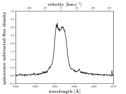
Figure 15: Spectrum with asymmetry for V388 Cas; the spectrum corresponds to entry no. 1 in Table The CARMENES search for exoplanets around M dwarfs.

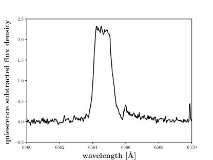
Figure 16: Spectrum with asymmetry for YZ Cet; the spectrum corresponds to entry no. 2 in Table The CARMENES search for exoplanets around M dwarfs.

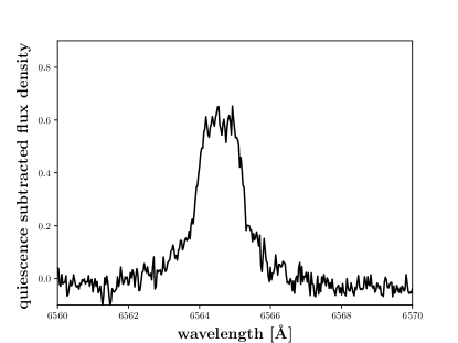
Figure 18: Spectrum with asymmetry for TZ Ari; the spectrum corresponds to entry no. 8 in Table The CARMENES search for exoplanets around M dwarfs.

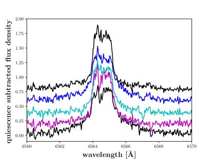
Figure 19: Spectra with asymmetry for GJ 166 C; from bottom to top the spectra correspond to entry nos. 9 – 13 in Table The CARMENES search for exoplanets around M dwarfs.

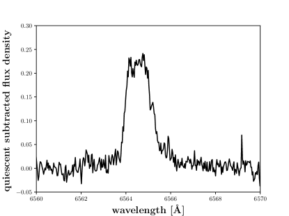
Figure 20: Spectrum with asymmetry for V2689 Ori; the spectrum corresponds to entry no. 14 in Table The CARMENES search for exoplanets around M dwarfs.

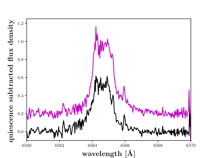
Figure 21: Spectra with asymmetry for G099-049; the spectrum corresponds to entry no. 15 in Table The CARMENES search for exoplanets around M dwarfs.

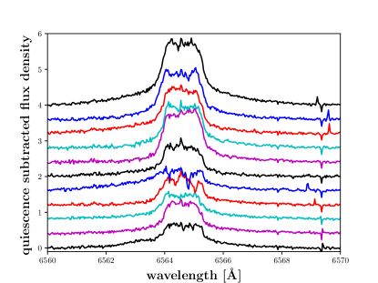
Figure 22: Spectra with asymmetry for YZ CMi; from bottom to top the spectra correspond to entry nos. 17 – 27 in Table The CARMENES search for exoplanets around M dwarfs.

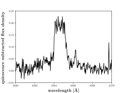
Figure 23: Spectrum with asymmetry for GJ 362; the spectrum corresponds to entry no. 28 in Table The CARMENES search for exoplanets around M dwarfs.

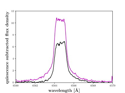
Figure 24: Spectra with asymmetry for CN Leo; from bottom to top the spectra correspond to entry nos. 29 – 30 in Table The CARMENES search for exoplanets around M dwarfs.

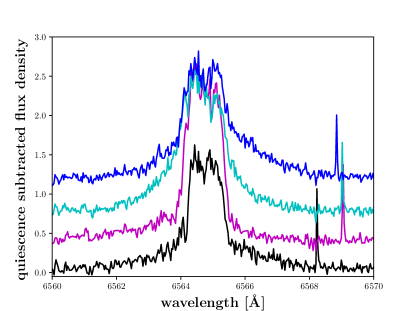
Figure 25: Spectra with asymmetry for WX UMa; from bottom to top the spectra correspond to entry nos. 31 – 34 in Table The CARMENES search for exoplanets around M dwarfs.

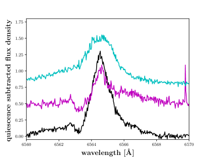
Figure 26: Spectra with asymmetry for StKM 2; from bottom to top the spectra correspond to entry nos. 35 – 37 in Table The CARMENES search for exoplanets around M dwarfs.

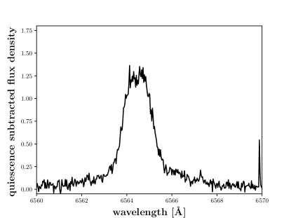
Figure 27: Spectrum with asymmetry for GL Vir; the spectrum corresponds to entry no. 38 in Table The CARMENES search for exoplanets around M dwarfs.

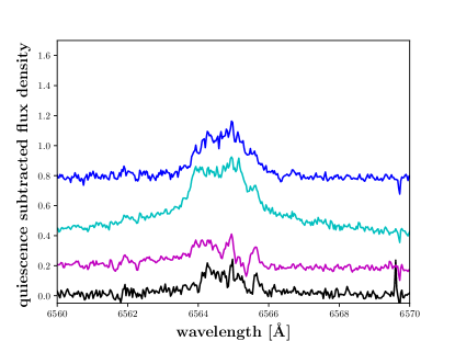
Figure 28: Spectra with asymmetry for OT Ser; from bottom to top the spectra correspond to entry nos. 39 – 42 in Table The CARMENES search for exoplanets around M dwarfs.

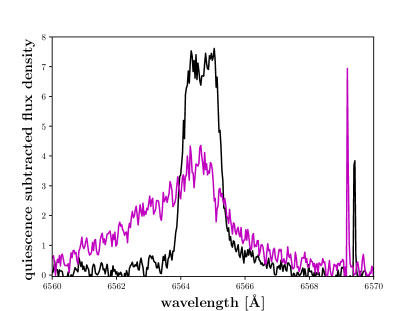
Figure 29: Spectra with asymmetry for vB 8; from bottom to top the spectra correspond to entry nos. 43 – 44 in Table The CARMENES search for exoplanets around M dwarfs.

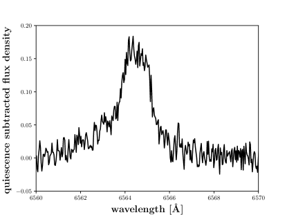
Figure 30: Spectrum with asymmetry for J18174+483; the spectrum corresponds to entry no. 45 in Table The CARMENES search for exoplanets around M dwarfs.

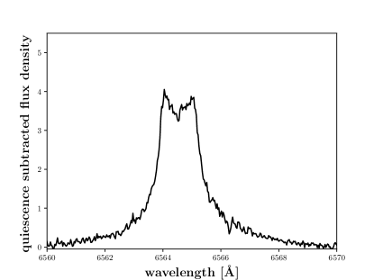
Figure 31: Spectrum with asymmetry for G141-036; the spectrum corresponds to entry no. 46 in Table The CARMENES search for exoplanets around M dwarfs.

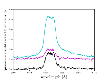
Figure 34: Spectra with asymmetry for GT Peg; from bottom to top the spectra correspond to entry nos. 65 – 67 in Table The CARMENES search for exoplanets around M dwarfs.

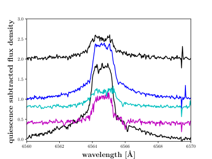
Figure 35: Spectra with asymmetry for J23548+385; from bottom to top the spectra correspond to entry nos. 68 – 72 in Table The CARMENES search for exoplanets around M dwarfs.

Appendix B Detected asymmetries in Na i D and He i D₃

We present here all Na i D and He i D₃ spectra with detected asymmetries with the quiescent spectrum subtracted and the best fit overlaid in Figs. 36 to 38.

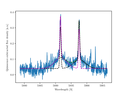
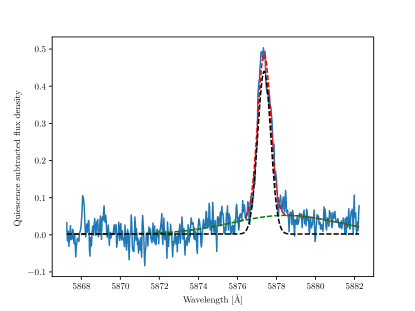
Figure 36: Spectrum with asymmetry for OT Ser.

Appendix C Detected asymmetries in He i 10833 Å  and corresponding excess fluxes in Pa$\beta$

Here we present all quiescent flux density subtracted spectra with a He i 10833 Å  broad wing in Figs. 39 to 46. We searched in all spectra exhibiting an H$\alpha$ asymmetry. The problem of the strong air glow and telluric lines in the region is apparent. Besides the broad wing spectra we also always present a quiescent spectrum. In the right panel we show the same for the corresponding Pa$\beta$ spectra. It is quite apparent that the line reacts in a much less sensitive manner. For both spectral lines we mark the reference central wavelength with a blue vertical line.

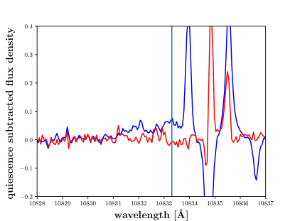
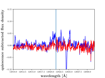
Figure 39: Spectrum with broad wing in He i 10833 Å  for V388 Cas in blue, a quiescent spectrum for comparison in red.

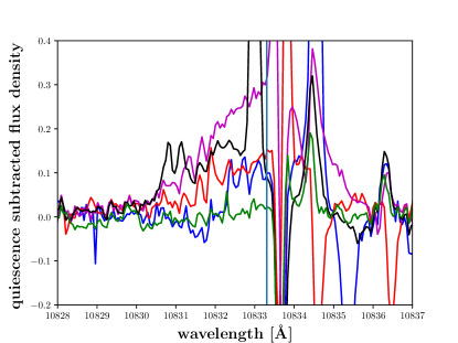
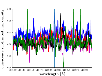
Figure 40: Spectrum with broad wing in He i 10833 Å  for Barta 161 12 in blue, black, red, and magenta, and a quiescent spectrum for comparison in green.

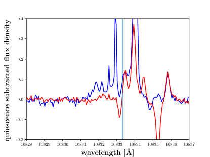
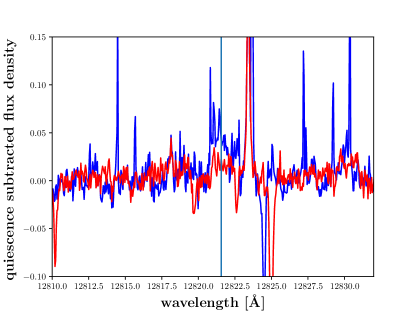
Figure 41: Spectrum with broad wing in He i 10833 Å  for CN Leo in blue, a quiescent spectrum for comparison in red.

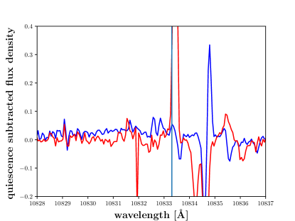
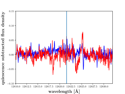
Figure 42: Spectrum with broad wing in He i 10833 Å  for StKM2-809 in blue, a quiescent spectrum for comparison in red.

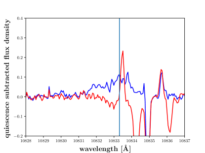
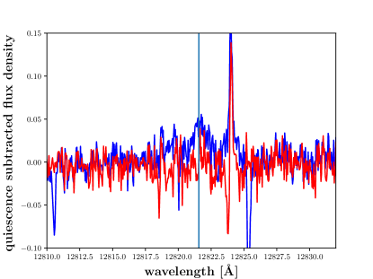
Figure 43: Spectrum with broad wing in He i 10833 Å  for OT Ser in blue, a quiescent spectrum for comparison in red.

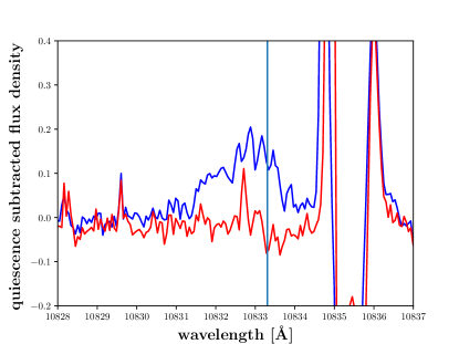
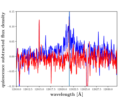
Figure 44: Spectrum with broad wing in He i 10833 Å  for G141-036 in blue, a quiescent spectrum for comparison in red.

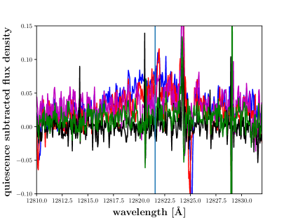
Figure 45: Spectra with broad wing in He i 10833 Å  for EV Lac, the green spectrum is the quiescent comparison spectrum.

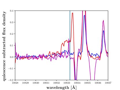
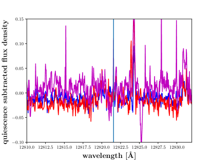
Figure 46: Spectra with broad wing in He i 10833 Å  for GT Peg, the magenta spectrum is the quiescent comparison spectrum.

Appendix D Examples of the H$\alpha$ profile fit for the weakest and strongest asymmetries

Here we present examples of our fits of the H$\alpha$ line profile. For each of the categories (i) red asymmetry, (ii) blue asymmetry, and (iii) symmetric broadening, we show the strongest and the weakest asymmetry and its fit.

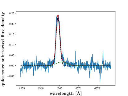
Figure 48: Weakest red asymmetry was found for V2689 Ori corresponding to asymmetry no. 14 in Table The CARMENES search for exoplanets around M dwarfs.

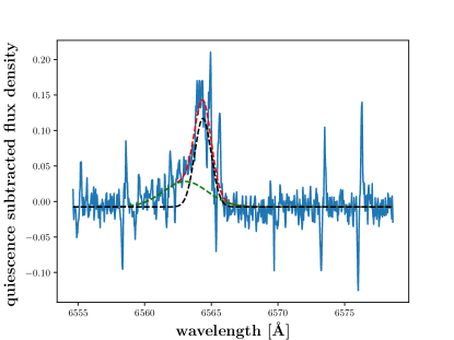
Figure 50: Weakest blue asymmetry was found for OT Ser corresponding to asymmetry no. 40 in Table The CARMENES search for exoplanets around M dwarfs.

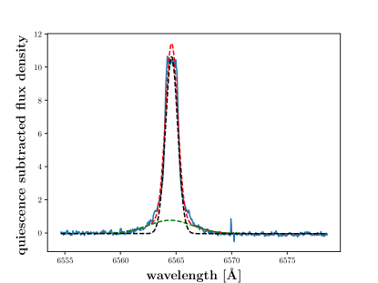
Figure 51: Strongest symmetric broadening was found for CN Leo corresponding to asymmetry no. 30 in Table The CARMENES search for exoplanets around M dwarfs.

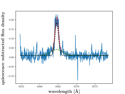
Figure 52: Weakest symmetric broadening was found for GJ 362 corresponding to asymmetry no. 28 in Table The CARMENES search for exoplanets around M dwarfs.