1.2in0.9in0.5in1.5in

Chapter 1 Introduction

In This days computer science communities Give more vigilance and focus for Quantum Algorithm Due to the Features it has and more affluent representation. mainly Because of they offer substantial speed-up over classical algorithms and furthermore have more affluent structure than classical counterparts .For example, Grover’s search [Gro96] algorithm is quadratically much quicker furthermore Shors factorization algorithm [Sho94] is also exponentially faster than renowned classical algorithms. Quantum algorithms furthermore have a more affluent structure than their classical counterparts since they use qubits rather than bits as the basic representational unit . I n this days Quantum walks have become a common well liked theme of study in different fields . The quantum computing community is interested in quantum walks due to the role it plays in certain algorithms. In quantum computing, quantum walks are the quantum analogue of classical random walks. Like the classical random walk, where the walker’s present state is described by a probability distribution over positions, the walker in a quantum walk is in a superposition of positions. The quantum walk differs from the classical walk in that its state vector is complex-valued rather than real-valued and its evolution is described by unitary rather than stochastic matrices. The evolution of the classical walk is random and a state vector can articulate the probabilities of all the likely outcomes. The evolution of the quantum walk, on the other hand, is deterministic and the randomness only manifests itself when measurements are made. That the state vector of the quantum walk is complex valued allows different routes in the walk to interfere, making amazingly different probability distributions on the vertices’s of the graph. Quantum walks have many applications in different areas of aspects. Among that I tried to show one of them and investigate how this well liked study theme is Feasible.

As we understand graph-based or Graphical advances are utilised extensively in computer vision areas . Much work has been concerned with developing effective graphical representations for diverse submissions and means of performing this tasks encompass exact and inexact graph equivalent , assessing graph distances , graph embedding and graph clustering broad variety of tasks utilising these representations . Some of the soonest work which made use of graphical representations of images was that carried out by Barrow and Popplestone[] and Fischler and Elschlager []. Their work demonstrated that high-level object acknowledgement could be achieved by representing images using graphs.

One of the most basic problem that we need to face in the graph domain is the of assessing likeness or the distance between the Graphs . How they are alike? Graph matching (GM) performances a central role in explaining correspondence problems in computer vision. thus I tried to investigate this well liked study area for this graph matching problems. These studies mostly consider attributed graphs. Graphs are routinely utilised as abstract representations for convoluted scenes, and numerous computer vision problems can be formulated as an attributed graph matching problem,where the nodes of the graphs represent features of the image and edges correspond to relational aspects between features (both nodes and edges can be attributed, i.e. they can encode characteristic/feature vectors). Graph matching/equivalent then comprises in finding a correspondence between nodes of the two graphs such that they look most alike when the vertices’s are labeled according to such a correspondence. An intriguing question arises in this context. If we are given two attributed graphs, let say G and G0, should the optimal match be uniquely determined? In this thesis I used Hungarian algorithm to find the cost and optimal between the matching i.e. minimum matching in terms of the cost of matching .The Hungarian algorithm allows a "minimum matching(optimal)" to be found.

In This paper I have to investigate the topic "How Continuous-time quantum walk (CTQW) or Quantum algorithm" can be directed for Graph matching problem .

1.1 Thesis Aim:

The aim of this study is to investigate one of the application of Quantum walks i.e. Quantum walks for graph matching .I introduce similarity measure between attributed graphs which is based on the evolution of continuous-time quantum walks .In specific, I mainly focused on the distance b/n the nodes and cost of the matching . Thus, given a pair of graph, i.e. attributed graph, then I conceived new structure by connecting edges of one graph to other. On this structure I defined two continues-time quantum walks which have density operators. Then to define this similarity assess, I used Quantum Jenson-Shannon Divergence, a assess which has been presented as a means to compute the distance between Quantums.then I utilised The Hungarian algorithm to find the optimal matching. Finally measuring the distance between two Graphs which might have different size and dimesions then classifying those Graphs by using nearest neighbour classification.

1.2 Thesis Overview:

The remainder of this thesis is coordinated as follows : chapter two provides brief overview and essential Introduction about quantum walks continues -time quantum walks, Random walks, Graph theory. In the third chapter i.e. methodology, I introduce the similarity measure and detailed overview how I did this research .In the fourth section I illustrate the experimental results and in the last chapter deduction is offered..

Chapter 2 Related Literature

A quantum walks are the quantum analogue of the classical random walks. In this thesis I Give , more focus only for continuous-time quantum walks. In this chapter I try to introduce the concept of a quantum walk, Continuous-time quantum walk (CTQW), Random walks, Graph theory. In Section 2.1, I presented basic notation, concepts and terminology of Graph especially the idea related to this thesis. In Section 2.2, I give an overview of random walk and then in section 2.3 I presented basic definitions and essential introduction to the rudimentary terminology needed to understand the suggested quantum framework like quantum walks and Continuous-time quantum walk (CTQW) and in the last part I recounted, about The Hungarian Algorithm and its significance.

2.1 Graph

Many real-world situations can conveniently be described by means of a diagram consisting of a set of points together with lines joining certain pairs of these points. For example, the points could represent people, with lines joining pairs of friends; or the points might be communication centres, with lines representing communication links. Notice that in such diagrams one is mainly interested in whether or not two given points are joined by a line; the manner in which they are joined is immaterial. A mathematical abstrac- tion of situations of this type gives rise to the concept of a graph.

Recently, several graph based approaches has been proposed to solve problems in computer vision and pattern recognition [TP18], authors in [ZDS12, DAS15, TZPP16, TZP⁺17, TP14] formulate multi-target tracking problem in a graph, visual geo-localization [ZTI⁺17, ZS10, ZS14] , outlier detections [ZTPP16], segmentation [ZAP16, ZAP17, ZP15] and so on.

A Graph, G, is defined as an organised pair formed from a set of vertices’s, V and a set E of edges. A forming set of edges is a subset of vertices’s, i.e. (x,y)$\varepsilon$V , where x and y are components of the set V . To be accurate , if the pair of A vertex in an edge is unordered, the graph we describe is then known as undirected. All the graph organisations we talk about will be this kind . An example of an undirected Graph is shown in fig.1.
We define the order of the graph to be the number of Vertices’s, V, and the size to be the number of edges, E. In fig.1.we can see that some vertices’s have more (or less) connections to other vertices’s than the other. The degree d of a vertex is defined as the number of edges incident upon it.Graphs offer a convenient way tocomprise diverse kinds of mathematical things.[5] Essentially, any graph is made up of two sets, a set of vertices and a set of Edges depending on the specific situation we are endeavouring to represent, although, we may desire to impose limits on the kind of Edge we allow. For some problems we desire the Edge to be directed from one vertex to another; while, in other ones the Edge are undirected
A graph G comprises of a finite set V (G) of vertices’s and a finite set of E (G) of edges.
* Each edge is associated with a set comprising of either one or two vertices’s ,endpoints
* An edge with just one endpoint is called a loop
* Two distinct Edge with the identical set of endpoints are said to be parallel.
* Two vertices’s that are connected by an edge are called adjacent.
* An Edge is said to be incident on each of its endpoints.
* Two Edge occurrence on the identical endpoint are adjacent.
* A vertex on which no edges are incident is isolated.
* A graph encompassing no vertices’s is called empty; and a graph with vertices’s is nonempty.

Figure 2.1: An example of a general, undirected graph. It consists of 5 vertices’s, of varying degree, and 6 edges

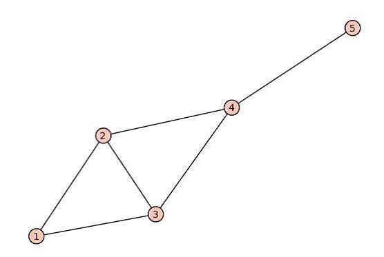
In this research paper , I only address graphs which have no self-loops. Most will be a single attached graph, that is there is a path, along edges, from any vertex to any other, i.e. there is one connected component. One way to characterise the connectivity of a structure is by the adjacency matrix. For a graph, G, of M vertices’s, this is a M$\times$ M matrix where the entries of the matrix, A_a,b, is nonzero if an edge exists between vertices’s a and b. In an undirected graph with no self loops, we characterise it

A_a,b= $\bigl{\{}_{0\ldots\ldots\ldots\ldots otherwise}^{1\ldots.........if\ldots\left\{a,b\right\}\in E}$

A similarity matrix of connectivity is the Laplacian of the graph. This can be defined as:

L=D-A_a,b                          (2.1)

where D_d is the diagonal matrix whose entries Da,a = d_a, where d_a is the degree of each vertex. As an example, you can see both the adjacency and Laplacian matrices of the graph in fig 2.2

Figure 2.2: the adjacency and Laplacian matrices of the above Graph

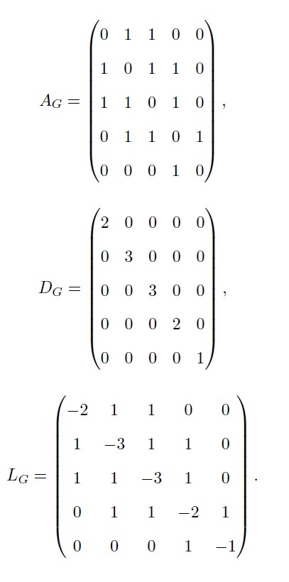
Graphical advances are utilised extensively in computer vision.Much work has been concerned with evolving effective graphical representations for diverse applications and means of accomplishing a wide variety of jobs using these representations. These jobs encompass exact and inexact graph equivalent, calculating graph distances and graph clustering . Some of the soonest work which made use of graphical representations of images illustrated that high-level object recognition could be accomplished by comprising images using graphs.

2.2 Random walks

Random walks are advantageous accoutrement in the assay of the structure of a Graphs. The stable state of the random walk on a graph is granted by the premier eigenvector of the transition probability matrix, and this in turn is related to the Eigen structure of the Laplacian matrix. therefore, the study of random walks has been the aim of maintained study activity in spectral graph theory. From a functional viewpoint, there have been a number of useful submissions of random walks . One of the most significant of these is the investigation of routing problems in network and circuit theory [THRP05] and more latest interest is the use of this notion for random walk by Brin and page [BP12]to characterise the page Rand index utilised by the Googlebot search engine [THRP05]. In the pattern recognition community, there have been some attempts to use random walks for graph matching . These include the work of Robles-Kelly and Hancock [RKH04, RKH05] which has used both a standard spectral method and a more complicated one based on concepts from graph seriation to alter graphs to strings, so that string matching procedures may be utilised to compare graphs. Gori, Maggini and Sarti [GMS05] on the other hand, have used ideas borrowed from Page Rank to associate a spectral index with the vertices’s of a graph and have then used standard attributed graph-matching procedures to agree the producing attributed graphs. Random walk methods have a close connection with graph spectral methods for image segmentation . For instance, Melia and Shi [MS01] have utilised random walks to reinterpret Shi and Maliks normalized cut method and continue the procedure to learn image segmentation. Grady has taken this work one step farther by evolving interactive segmentation schemes founded on the anticipations of random walks. At a higher level, Zhu, Ghahramani and Laerty [RKH05] have performed semi supervised learning utilising random walks on a marked/labeled graph structure. Borgwardt et al. have evolved a kernel that preserves the path length circulation of a random walk on a graph, and have utilised this to analyses protein data . This kernel has been utilised by Neuhaus and Bunke to kernelise the computation of graph edit distance and assess the similarity of graphs. eventually, Qiu and Hancock [QH07] have shown how the commute times of random walks can be used to render graph spectral clustering algorithms robust to edge weight errors, and have discovered the submission of the method to image segmentation, multimode motion tracking and graph matching. The commute time permits the vertices of a graph to be embedded in a low-dimensional space, and the geometry of this embedding permits the vertices’s to be clustered into disjoint subsets. A random walk consists of two constituents: a states space on which at, any point in time, there is a probability distribution giving the position of the walk, and a transition function which give the probabilities for transitions between one state and another. As such, random walks are most naturally defined on graphs since the connectivity structure of a graph defnes which transitions are allowed. Additionally, weighted graphs can be utilised if the walk is to be biased in some way. Given a graph and a starting point we select a neighbor of it at random and move to this neighbor ; then we select a neighbor of this point at random and move to it etc. The (random) sequence of points selected this way is a random walk on the graph. A random walk is a finite Markov chain of links that is time reversible In fact, there is not much difference between the idea of random walks on graphs and the idea of finite Markov chains; every Markov chain can be viewed as random walk on a directed graph if we permit weighted edges. likewise time reversible Markov chains can be viewed as random walks on undirected graphs and symmetric Markov chains,as random walks on regular symmetric graphs. Random walks are a model of diffusion which are important in, amongst other areas, statistical physics, applied probability and randomized algorithms .

Let G=(V, E) be a connected graph with n nodes and m edges. Consider a random walk on G we start at a node v₀ if at the t-th step we are at a node v_t we move neighbor of v_t with probability $\frac{1}{d(v_{t})}$ Clearly, the sequence of random nodes (v_t: t=0,1…) is a Markov chain.The node v₀ may be fixed but may itself be drawn from some initial distribution P₀ . We denote by Pt the distribution of vt

P_t(i) = Prob (v_t= i)                         (2.2)

We denote by M= (p_i,j)i,j$\in$V the matrix of transition probabilities of this Markov chain. So

                              p_i,j= $\bigl{\{}_{0\ldots\ldots\ldots\ldots otherwise}^{1/d(i)\ldots if\ldots i,j\in E}$

(2.3)

Let A_G be the adjacency matrix of G and let D denote the diagonal matrix with (D)_ii=1/d(i) then M= DA_G. If G is d-regular, then M=(1/d)A_G. The rule of the walk can be expressed by the simple equation:

P_t+1=M^TP_t                                     (2.4)

(the distribution of the t-th point is viewed as a vector in R^v), and hence:

P_t=(M^T)^tP₀                           (2.5)It follows the probability p_i,j^tthat starting at i we reach j in t steps is given by the i,j entry of the matrix M^t

2.3 Quantum walks

Quantum walks have been presented as quantum equivalent of random walks,and a good recent review of their properties is given by Kempe [Kem03]. The behavior of quantum walks is ruled by unitary ratherthan stochastic matrices. The stochastic matrix of a classical random walk is such that its columns sum to unity. A unitary matrix, on the other hand, has convoluted applications. For a unitary matrix the squares of the entries in the columns sum to unity. Quantum walks possess a number of interesting properties not displayed by classical random walks. For example, because of the evolution of the quantum walk is unitary and therefore reversible, the walks are non-ergodic, and what is more, they do not have a limiting distribution. Quantum walks provide an approach to designing quantum algorithms that lends itself more to physical intuition.There are two different models for the quantum random walk, both of which can be simulated on an arbitrary graph. The first of these is the continuous-time quantum walk proposed by Fahri and Guttmann [FG98]. The evolution of the walk is then granted by Schrodinger equation. Fahri and Guttmann [FG98] show that if a classical Markov process is able to penetrate a family of trees in polynomial time, then the quantum walk that they define is also able to. They go on to give an example of a family of trees that cannot be penetrated in polynomial time by the classical Markov process but can be by their quantum walk. Unfortunately, they are not able to use this walk to construct a solution to any classically hard problems. By making use of the exponentially faster hitting times that are discerned for continuous-time quantum walks on graphs.An exponential speedup for the hitting time was also furthermore discerned by Kempe [AAKV01] for the discrete-time quantum walk. The discrete time quantum walk is the quantum analogue of the classical random walk. The quantum type of the discrete-time quantum walk on an random graph was formalized by Aharonov, Ambainis and Kempe [AAKV01]. Kempe considered the walk on the n-dimensional Hypercube and was able to show that the hitting time from one vertex to the one opposite is polynomial in n . In general, the discrete-time quantum walk is not effortlessly analyzed. Kempe Was able to do so for the hypercube due to its regular structure. She demonstrates how this polynomial hitting time could be of use for a routing problem, and also, in a later paper, shows that it could be used to solve the 2-SAT problem effieciently (note that this problem can also be explained effciently using a classical algorithm). The many interesting properties exhibited by quantum walks,and the fact that their behavior is dictated by the structure of the graphs supporting them, proposes that they could be a very helpful tool for graph analysis. Having said this, there are, as yet,few algorithms for graph matching based on quantum random ‘walks. One approach is that proposed by Gudkov [GN02].who suggested modeling the graph as a set of point particles with an attractive force between adjacent vertices’s. The system is developed from a set initial state and the set of ordered separation distances calculated. They conjecture that this approach explains the graph isomorphism problem.

2.1.1 A Continuous-time quantum walk (CTQW)         
         Like the classical random walk on a graph, the state-space of the continuous-time quantum walk is the set of vertices’s of the graph. although, the probability of being at a certain state is given by the square of the amplitude of that state, rather then just the amplitude of the state (as is the case classically). This permit/allows destructive as well as constructive interference to take place. a walk on a given connected graph that is dictated by a time-varying unitary matrix that relies on the Hamiltonian of the quantum system and the adjacency matrix. CTQW belongs to what is renowned as Quantum walks, which also consists of the Discrete-time quantum walk.

A continuous-time quantum walk (CTQW) on a graph G = (V,E), where V is the set of vertices’s (nodes) and E is the set of edges connecting the nodes, is defined as follows: Let A be the of adjacency matrix of G with elements

A_u,v= $\bigl{\{}_{0\ldots\ldots\ldots\ldots otherwise}^{1\ldots.........if\ldots\left\{u,v\right\}\in E}$                       (2.6)

D be the degree matrix of G (for which the diagonal entry corresponding to vertex v is degree (v)), and let L = D - A, be the corresponding Laplacian matrix which is postive semi definite. The continuous-time quantum walk on the graph G is then defined by the unitary matrix

U(t)=$e^{-itL}$                                          (2.7)

Where i is the imaginary unit and t for time.

The evolution of the walk is then given by Schrodinger equation, where we take the Hamiltonian of the system to be the graph Laplacian, which yields

$\frac{d}{dt}$$|\psi_{t}>$ = -iL$|\psi_{t}>$                                 (2.8)

Given an initial state $|\psi_{0}>$, we can solve Equation 2.8 to determine the state vector at time t.

$|\psi_{t}>$=e^iLt$|\psi_{0}>$                                (2.9)

Given the Laplacian matrix we can compute its spectral decomposition L = $\Phi\Lambda\Phi^{T}$ , where $\Phi$ is the n$\times$n matrix $\Phi$= ($\Phi_{1}$|$\Phi_{2}$|$\ldots|\Phi_{n}$) with the ordered eigenvectors as columns and $\Lambda$ = diag($\Lambda{}_{1}$,$\Lambda{}_{2}$,$\ldots$$,\Lambda{}_{n}$) is the n$\times$ n diagonal matrix with the ordered eigenvalues as elements, such that 0 = $\Lambda$₁$\leq$$\Lambda_{2}$$\leq$$\ldots\leq\Lambda_{n}$.Using the spectral decomposition of the Graph Laplacian and the fact that   exp[-iLt] = $\Phi^{T}$exp[-i$\Lambda$t] $\Phi$ , we can finally write

$|\psi_{t}>$ = $\Phi^{T}$e^-iΛt$\Phi$$|\psi_{0}>$                      (2.10)

2.4 The Hungarian Algorithm

The Hungarian algorithm is an algorithm for explaining a matching difficulty or more generally an assignment linear programming difficulty. The name was granted by H.W.Kuhn in acknowledgement of the work of the two mathematicians J.Egervary and D.Konig. The Hungarian Algorithm is actually a exceptional case of the Primal-Dual Algorithm. It takes a bipartite graph and makes a maximal matching..                          
The Hungarian Algorithm:
1. Set S $\leftarrow$ $\emptyset$. (We can furthermore use some other initial matching.)
2. If every vertex in V₁ or in V₂ is agreed in S, then S is a maximum matching and we halt.
3. If there are unmatched vertices’s in S of V₁, then go through them in some order constructing alternating trees (the procedure of building is not significant as we claimed). If there is an augmenting tree, then augmenting the matching S by utilising the augmenting path we have another matching S1. Set S $\leftarrow$ S₁ and go to 2.
4. If all the alternating trees that have unmatched vertices’s in V₁ as roots are Hungarian, S is maximal and we halt.

Chapter 3 Methodologies

Quantum walks are the quantum analogue of classical random walks. I emphasized only continues-time quantum walks. Given a graph G= (V, E), the state space of the continuous -time quantum walkS defined on G is the set of the vertices’s V of the graph. Unlike the classical case, where the evolution of the walker conducted by stochastic matrix (i.e. a matrix whose columns sum to unity), in the quantum case the dynamics of the walker is ruled by a complex unitary matrix i.e. the matrix that multiplied by its conjugate transpose yields the identity matrix. therefore the evolution of the walk is reversible which suggests that quantum walks are non-ergodic and do not possess a limiting distribution. G = (V,E), where V is the set of vertices’s (nodes) and E is the set of edges connecting the nodes, is defined as follows: Let A be the of adjacency matrix of G with elements

A_u,v= $\bigl{\{}_{0\ldots\ldots\ldots\ldots otherwise}^{1\ldots.........if\ldots\left\{u,v\right\}\in E}$                       (3.1)

D be the degree matrix of G (for which the diagonal entry corresponding to vertex v is degree (v)), and let L = D - A, be the corresponding Laplacian matrix . The continuous time quantum walk on the graph G is then defined by the unitary matrix

U(t)=$e^{-itL}$                                          (3.2)

Where i is the imaginary unit and t for time.

The evolution of the walk is then given by Schrodinger equation, where we take the Hamiltonian of the system to be the graph Laplacian, yields

$\frac{d}{dt}$$|\psi_{t}>$ = -iL$|\psi_{t}>$                                 (3.3)

Given an initial state $|\psi_{0}>$, we can solve Equation 2.8 to determine the state vector at time t.

$|\psi_{t}>$=e^iLt$|\psi_{0}>$                                (3.4)

Given the Laplacian matrix we can compute its spectral decomposition L = $\Phi\Lambda\Phi^{T}$ , where $\Phi$ is the n$\times$n matrix $\Phi$= ($\Phi_{1}$|$\Phi_{2}$|$\ldots|\Phi_{n}$) with the ordered eigenvectors as columns and $\Lambda$ = diag($\Lambda{}_{1}$,$\Lambda{}_{2}$,$\ldots$$,\Lambda{}_{n}$) is the n$\times$ n diagonal matrix with the ordered eigenvalues as elements, such that 0 = $\Lambda$₁$\leq$$\Lambda_{2}$$\leq$$\ldots\leq\Lambda_{n}$.Using the spectral decomposition of the graph Laplacian and the fact that   exp[-iLt] = $\Phi^{T}$exp[-i$\Lambda$t] $\Phi$ , we can finally write

$|\psi_{t}>$ = $\Phi^{T}$e^-iΛt$\Phi$$|\psi_{0}>$                      (3.5)

Quantum Jenson Shannon Divergence:-A pure state can be described by the vector $|\psi_{i}>$.The generalization of probability distributions on density matrices allows to define quantum Jensen Shannon divergence (QJSD). the system is said to be the ensemble of pure states {$|\psi_{i}>$,P_i} . The density operator(or density matrix) of such a scheme is defined as

$\rho$=$\sum_{i}$ p_i$|\psi_{i}>$$<\psi_{i}|$                     (3.6)

The Von Neumann entropy of a density operator$\rho$ is:

H_N($\rho$)= -Tr($\rho$$\log$$\rho$)= -$\sum_{j}$ $\lambda_{j}$ $\log$$\lambda_{j}$                     (3.7)

where $\lambda_{j}$s are the Eigen values of $\rho$. on the basis of the Von Neumann entropy , I can use Quantum Jensen Shannon divergence(QJSD) b/n the density operators $\rho$ and $\sigma$ as the Two probability distributions let say $\rho$ = (p1,$\ldots,$ pn) and $\sigma$ = (q1,$\ldots$,qn)on a finite alphabet of size n $\geq$2,Quantum Jensen-Shannon divergence(QJSD) is a measure of divergence between P and Q. It measures the deviation between the Shannon entropy of the mixture ($\rho$ +$\sigma$)/2 and the mixture of the entropies, and is given by:- .

QJSD($\rho$,$\sigma$) = H_N$\left(\frac{\rho+\sigma}{2}\right)$-$\frac{1}{2}$H_N$\left(\rho\right)$-$\frac{1}{2}$H_N$\left(\sigma\right)$                        (3.8)

This quantity is always well defined , symmetric and negative definite.It can also be shown that QJSD($\rho$,$\sigma$) is bounded ,i.e

                                     0$\leq$ QJSD($\rho$,$\sigma$)$\leq$1                        (3.9)

Figure 3.1: Given two graphs G₁(V₁,E₁) and G₂(V₂,E₂), I build a new graph G=(V,E) where V=V₁$\cup$V₂,,E=E₁$\cup$E₂$\cup$E₁₂ and we add a new edge(u,v) between each pair of nodes u$\epsilon$V₁ and v$\epsilon$V₂

3.1 A likeness Measure for Attributed Graphs

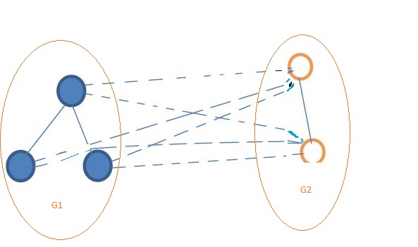
Granted two graphs G₁(V₁,E₁) and G₂(V₂,E₂). I construct a new graph G=(V,E)where V=V₁$\cup$V₂, E=E₁$\cup$E₂$\cup$E₁₂ and (u,v)$\epsilon$E₁₂ onlyif u$\epsilon$ V₁ and v$\epsilon$V₂. To hand this new structure , I define two continuous-time quantum walks
$|\psi_{t}$${}^{-}>$= $\sum_{u\epsilon V}$$\psi_{0u}^{-}|u>$ and $|\psi_{t}$${}^{+}>$= $\sum_{u\epsilon V}$$\psi_{0u}^{+}|u>$ on G with starting states.,
     $|\psi_{0u}^{-}>$=$\left\{\frac{+\frac{d_{u}}{C}.......if....u\epsilon G_{1}}{-\frac{d_{u}}{C}.......if......u\epsilon G_{2}}\right\}$                       $|\psi_{0u}^{+}>$=$\left\{\frac{+\frac{d_{u}}{C}.......if....u\epsilon G_{1}}{+\frac{d_{u}}{C}.......if......u\epsilon G_{2}}\right\}$                       (3.10)

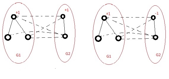
where d_u is the degree of the node u and C is the normalization constant such that the probabilities sum to one .Note that the walk will spread at a speed proportional to the edge weights, which means that given an edge(u,v)$\epsilon$E₁₂, the more similar V₁(u) and V₂(v) are , the faster the walker will propagate along the inter graph connection (u,v).
on the other hand , the intra-graph connection weights , which are not dependent on the nodes similarity , will not affect the propagation speed. Given this setting , allows the two quantum walks to evolve until a time T and we define the average density operators $\rho$_T and $\sigma$_T over this time as

$\rho$_T=$\frac{1}{T}$$\intop_{0}^{t}$$|\psi_{t}$${}^{-}>$$<\psi_{t}$${}^{-}|$dt          $\sigma$_T=$\frac{1}{T}$$\intop_{0}^{t}$$|\psi_{t}$${}^{+}>$$<\psi_{t}$${}^{+}|$dt                        (3.11)

In other words, I have to defined two mixed systems with equal probability of being in any of the pure states defined by the evolution of the quantum walks. then i will prove that, Graph G1 and Graph G2 are isomorphic , the Quantum Jenson-shannon divergnce between $\rho$_T and $\sigma$_T will be maximum,i.e it will be equal to 1.hence ,we can use this divergence scheme for measuring the similarity between two graphs .

Figure 3.2: Given two graphs which has different Inital point

3.2 QJSD for attributed Graphs

Given a pair of two attributed graphs G1, G2, then define the quantum Jensen-shannon Divergence between them as follows:

QJSD(G1,G2)=D_JS($\rho$_T,$\sigma$_T)                        (3.12)

where $\rho$_T and $\sigma$_T are the density operators defined as in Eq 3.11
corollary1 . given a pair of graphs G₁ and G₂ then QJSD between those graphs satisfies the following property
                                    0 $\leq$ QJSD(G₁,G₂)$\leq$ 1                        (3.13)

proof. according Eq. 3.12 the QJSD between G₁ and G₂ is defined as the quantum Jenson-Shannon divergence between two density operators and the value of quantum Jenson-Shannon divergence is bounded between 0 and 1 .

3.3 QJSD calculation/estimation

In this section I showed that the solution to Eq 3.12 can be Computed analytically, Particularlly how i did it computationaly .Recall that $|\psi_{t}>$=e^iLt$|\psi_{0}>$, then i rewrite Eq. as
                            $\rho_{T}$=$\frac{1}{T}$$\intop_{0}^{t}$ e^-iAt$|\psi$${}_{0}>$$<\psi$${}_{0}|$ e^-iAtdt                        (3.14)
since e^-iAt=$\Phi$e^-iAt$\Phi^{T}$, we can rewrite the previous equation in terms of the spectral decomposition of the adjacency matrix,
                            $\rho_{T}$=$\frac{1}{T}$$\intop_{0}^{t}$ $\Phi$e^-iAt$\Phi^{T}$$|\psi$${}_{0}>$$<\psi$${}_{0}|$ $\Phi$e^-iAt$\Phi^{T}$ dt                        (3.15)
The(r,c)element of $\rho$_T can be computed as
                            $\rho_{T}$(r,c)=$\frac{1}{T}$$\intop_{0}^{t}$($\Sigma$_k$\Sigma$_l$\phi$_rke${}^{-i\lambda_{k}t}$$\phi_{lk}$$\psi_{0l}^{-}$)
                                       =($\Sigma$_m$\Sigma$_n$\psi_{0m}^{+}$$\phi_{mn}$e${}^{-i\lambda_{n}t}$$\phi_{cn}$)dt                                (3.17)

let $\psi$_k=$\Sigma$_l$\phi$_lk$\psi$_0l and $\psi$_n= $\Sigma$_m$\phi$_mn$\psi$_0n⁺ then
                            $\rho_{T}$(r,c)=$\frac{1}{T}$$\intop_{0}^{t}$($\Sigma$_k$\phi$_rke${}^{-i\lambda_{k}t}$$\psi_{k}$$\Sigma$_n$\phi$_cne${}^{-i\lambda_{n}t}$$\psi_{n})$                                (3.18)
which can be finally rewritten as
$\rho_{T}$(r,c)=$\Sigma$_k$\Sigma$_n$\phi$_rk$\phi$_cn$\psi_{k}$$\psi_{n}$$\frac{1}{T}$$\intop_{0}^{t}$e${}^{i(\lambda_{n}-\lambda_{k})t}$dt.                               (3.19)

If we let T $\rightarrow$ $\infty$, Eq.3.19 further simplifies to

$\rho_{T}$(r,c)=$\Sigma$_λ$\Sigma$_kϵλ$\Sigma$_nϵλ$\phi$_rk$\phi$_cn$\psi_{k}$$\psi_{n}$

Chapter 4 Experimental Results

In this part, I evaluate the performance of the proposed approach and try to compare it with the value they have. The estimation I utilised for this enquiry is Quantum Jenson-Shannon Divergence value got by connecting two suggested( corresponding) node in the given time . I did a sequence of experiments on Different attributed graph and yields a worth b/n O and 1. for doing this experiment basically I used two Graph datasets (i.e COIL AND GRAPHS ) but among the two dataset I usually do this computation on the coil dataset , b/c it has more objects i.e 100 objects, with 72 views for each object. than the other one , therefore most of the tabular output that I putted here is comes from this data set .

4.1 Synthetic Data

I start by assessing the suggested approach on set of synthetically developed graphs. I developed 3 different weighted graph with different size and dimenastion . I took this weighted graph from coil dataset. In this dataset there is 100 objects with 72 views for each objects To this end , I randomly developed 3 different weighted graph prototypes with size 10, 20, 40 respectively .with this synthetic graphs to hand, then try to connect two Graph lets G and G0 (connect mean just make a connection b/n every vertice of G to every vertice of G0) this connection yields one graphs G1 as you can seen in fig.4.4.

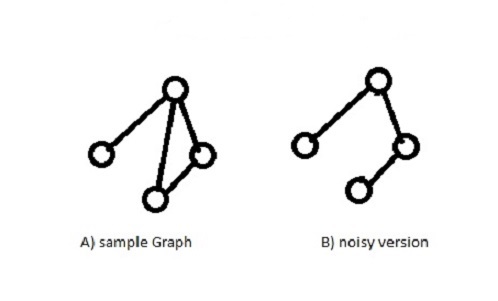
then after by utilising QJSD estimation schema I calculated QJSD between two Nodes found in different Graphs and I used Hungarian algorithm ,to know the cost and assignment of those graphs then I showed the optimal assignment between G and G0 in a tabular way. . fig 4.2 shows the distance (QJSD) b/n the node’s of the two graphs with different time interval . beside this I randomly pick a graph belonging to one class i.e among the 100 ones and I computed noisy version of that sample Graph. The nosie is applied to the edges only ,i.e adding or deleting edges, you can see in fig 4.1. then compute QJSD between G and its corrupted versions and plot it against time , the figure 4.1 shows .computed QJSD between G1 which has 30 nodes and its corrupted versions with limited time and second one with out limit.(i.e T$\rightarrow\infty$)

Figure 4.1: Sample Graph and its noisy version

Figure 4.2: QJSD measurement with different time in a given Graph and its noisy version , the first one in limited the value of time and the second one without

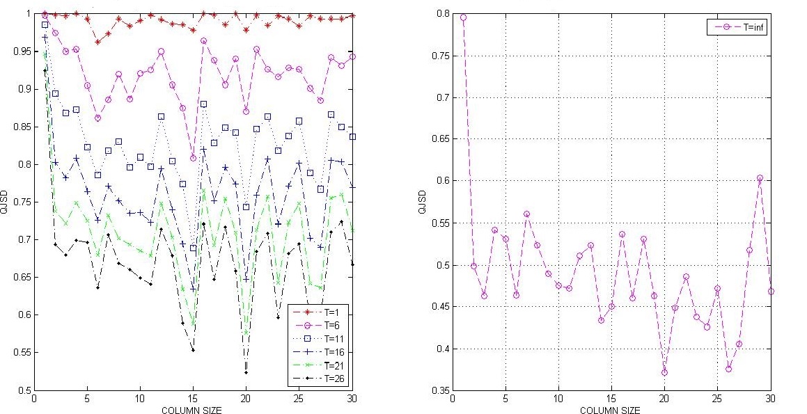
This specific tabular output with noise value of 3(three)(i.e adding or deleting 3 edge) to show the effect at different points(at different columan) I took the first Row and putted along with time difference

Figure 4.3: QJSD between two nodes found in Different Graphs with different values of time

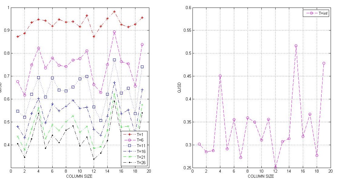
fig 4.2 shows the distance (QJSD) b/n the node’s of the two graphs with different time .i.e i selected two Graphs structure from Coil Dataset. then i connected and making one graphs G . then after by using QJSD measurement schema I calculated QJSD between two nodes found in different graphs and as i did in the previous one i took the first row and putted in tabular form along with time difference.

Figure 4.4: Making One Graph by connecting vertices’s of two graphs

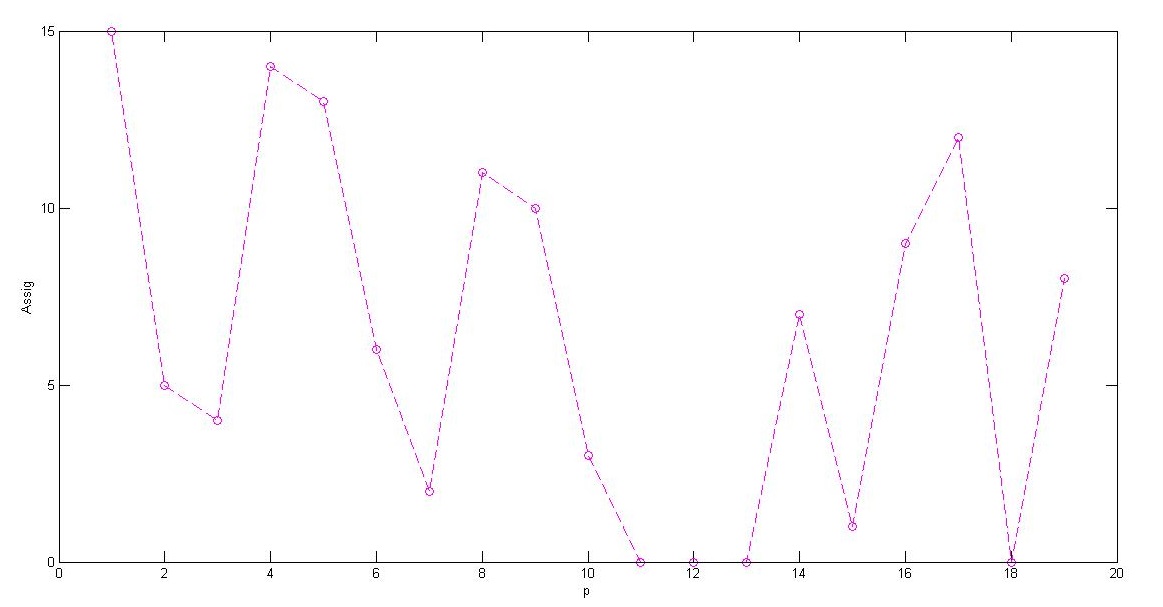
Fig 4.3 I selected two Graphs structure from Coil Dataset. then i connected and making one graphs G . then after by using QJSD measurement schema i calculated QJSD between two Nodes found in different Graphs and i used Hungarian algorithm to know the cost and assignment of those graphs then I tired to show optimal assignment between G and G0 in a tabular way .

Figure 4.5: Optimal Assignment between Different Graphs G1 and G2,

A crucial aspect of matching and recognition problems involves determining a suitable similarity measure between things. In numerous applications it is needed that such a assess possesses certain properties. In specific it is often desired that a distance assess d fulfills the following properties

• d(A, B) $\geq$ 0 (non negativity)
 • d(A, A) = 0 (identity)
 • d(A, B) = 0 $\Leftrightarrow$A = B (uniqueness)^a
 • d(A, B) = d(B, A) (symmetry)
 • d(A, B) + d(B, C) $\geq$d(A, C) (triangle inequality).

A distance function satisfying these five properties is called a metric [THRP05]

As second experiment , after knowing the QJSD Value b/n two nodes of two distinct graphs and b/n one graph and its noisy version. I should do some experiment pertaining with how this graphs are similar? In alignment to check that ,first i should calculate their distance with some formulas then classify those Graphs .The distance between the graph spectra is computed as pursues .for each graph G and G0 with adjacency matrix A, what i was doing for this experiment is xoring the two graphs and summing, when i did this may be the graphs has different dimensions or different lengths , therefor the vector are all made to be the same length by padding zeros to the end of the shorter vector.this yields The (i,j)th element of the distance matrix .

d(G₁,G₂) = 1 - $\frac{W(G_{12)}}{max(|G_{1}|,|G_{2}|)}$                               (4.1)

W₁₂=$\frac{\Sigma_{{}_{e1,e2}}xor(G_{1}(e1),G_{2}(e2))}{C(M,2)}$                               (4.2)
where
W₁₂= The weight between the Connected Graph
G₁ = Graph1
   G₂ = Graph2
M (The Number of Possible Edge b/n the Crossponding Nodes) = n(n-1)/2
n=Number of Nodes

After knowing the distance between the two Graphs by using the above formula I used the k-nearest neighbor (k-NN) method for classifying those graph based on closest training examples in the feature space. The nearest-neighbor procedure is perhaps the simplest of all algorithms for predicting the class of a test example. The training phase is trivial , simply store every training example, with its label. To make a prediction for a test example, first compute its distance to every training example. Then, keep the k closest training examples, where k $\geq$ 1 is a fixed integer. Look for the label that is most common among these examples. This label is the prediction for this test example.KNN has been involved in much research because of its simple calculation .

A major benefit of the kNN method is that it can be used to predict labels of any type.for example the training and test examples belong to some set X, while labels belong to some set Y . The common datasets which have been frequently used in the literature for evaluating this classification are COIL dataset.this dataset consists of 100 objects(class) with 72 views for each objects . when I did this experiment I selected sets as a traning set (50)and test set (50) randomly from different class of COIL DATASET AND yields 20 percent of the test data misclassified the rest classified properly.

Chapter 5 Conclusion

In this paper ,I have introduce new way of Graph Matching on attributed Graphs Specifcally I tried to investigate this proposed approch by utilising the time evolution of Continuous-time quantum walk i.e I conceive new structure by connecting edges of one graph to other. On this structure I define two continues-time quantum walks which have density operators. On this Given pair of Graphs I computed the quantum Jenson-shannon divergence .This yields the quantum Jensen-shannon Divergence b/n those Graphs Node’s then by using after this I used The Hungarian method that solves the assignment problem in polynomial time. then finding optimal assignement between those graphs Beside that Finding the Cost associated to Matching. In addition to this ,Ii did some Experiment pertaining/related to How this graphs are alike? In order to verfiy that ,first i should compute their distance with the overhead mentioned equations then classify those Graphs by using k-nearest neighbor (k-NN) method . Future work will be aim on revising time parameter more in deepness and furthermore assessing the performance by utilising distinct assessing schema.

References

- [AAKV01] Dorit Aharonov, Andris Ambainis, Julia Kempe, and Umesh Vazirani. Quantum walks on graphs. In Proceedings of the thirty-third annual ACM symposium on Theory of computing, pages 50–59. ACM, 2001.
- [Amb07] Andris Ambainis. Quantum walk algorithm for element distinctness. SIAM Journal on Computing, 37(1):210–239, 2007.
- [BP12] Sergey Brin and Lawrence Page. Reprint of: The anatomy of a large-scale hypertextual web search engine. Computer networks, 56(18):3825–3833, 2012.
- [DAS15] Afshin Dehghan, Shayan Modiri Assari, and Mubarak Shah. GMMCP tracker: Globally optimal generalized maximum multi clique problem for multiple object tracking. In IEEE Conference on Computer Vision and Pattern Recognition (CVPR), pages 4091–4099, 2015.
- [FG98] Edward Farhi and Sam Gutmann. Quantum computation and decision trees. Physical Review A, 58(2):915, 1998.
- [GMS05] Marco Gori, Marco Maggini, and Lorenzo Sarti. Exact and approximate graph matching using random walks. IEEE transactions on pattern analysis and machine intelligence, 27(7):1100–1111, 2005.
- [GN02] Vladimir Gudkov and Shmuel Nussinov. Graph equivalence and characterization via a continuous evolution of a physical analog. arXiv preprint cond-mat/0209112, 2002.
- [Gro96] Lov K Grover. A fast quantum mechanical algorithm for database search. In Proceedings of the twenty-eighth annual ACM symposium on Theory of computing, pages 212–219. ACM, 1996.
- [Kem03] Julia Kempe. Quantum random walks: an introductory overview. Contemporary Physics, 44(4):307–327, 2003.
- [MS01] Marina Meila and Jianbo Shi. A random walks view of spectral segmentation. 2001.
- [QH07] Huaijun Qiu and Edwin R Hancock. Clustering and embedding using commute times. IEEE Transactions on Pattern Analysis and Machine Intelligence, 29(11), 2007.
- [RKH04] Antonio Robles-Kelly and Edwin R Hancock. String edit distance, random walks and graph matching. International Journal of Pattern Recognition and Artificial Intelligence, 18(03):315–327, 2004.
- [RKH05] Antonio Robles-Kelly and Edwin R Hancock. Graph edit distance from spectral seriation. IEEE transactions on pattern analysis and machine intelligence, 27(3):365–378, 2005.
- [Sho94] Peter W Shor. Algorithms for quantum computation: Discrete logarithms and factoring. In Foundations of Computer Science, 1994 Proceedings., 35th Annual Symposium on, pages 124–134. Ieee, 1994.
- [SKW03] Neil Shenvi, Julia Kempe, and K Birgitta Whaley. Quantum random-walk search algorithm. Physical Review A, 67(5):052307, 2003.
- [THRP05] Andrea Torsello, Dzena Hidovic-Rowe, and Marcello Pelillo. Polynomial-time metrics for attributed trees. IEEE Transactions on Pattern Analysis and Machine Intelligence, 27(7):1087–1099, 2005.
- [TP14] Yonatan Tariku Tesfaye and Marcello Pelillo. Multi-target tracking using dominant sets. M.Sc. thesis, Università Ca’Foscari Venezia, 2014.
- [TP18] Yonatan Tariku Tesfaye and Andrea Prati. Applications of a graph theoretic based clustering framework in computer vision and pattern recognition. 2018.
- [TZP+17] Yonatan Tariku Tesfaye, Eyasu Zemene, Andrea Prati, Marcello Pelillo, and Mubarak Shah. Multi-target tracking in multiple non-overlapping cameras using constrained dominant sets. arXiv preprint arXiv:1706.06196, 2017.
- [TZPP16] Yonatan Tariku Tesfaye, Eyasu Zemene, Marcello Pelillo, and Andrea Prati. Multi-object tracking using dominant sets. IET computer vision, 10:289–298, 2016.
- [ZAP16] Eyasu Zemene, Leulseged Tesfaye Alemu, and Marcello Pelillo. Constrained dominant sets for retrieval. In 23rd International Conference on Pattern Recognition, ICPR 2016, Cancún, Mexico, December 4-8, 2016, pages 2568–2573, 2016.
- [ZAP17] Eyasu Zemene, Leulseged Tesfaye Alemu, and Marcello Pelillo. Dominant sets for "constrained" image segmentation. CoRR, abs/1707.05309, 2017.
- [ZDS12] Amir Roshan Zamir, Afshin Dehghan, and Mubarak Shah. Gmcp-tracker: Global multi-object tracking using generalized minimum clique graphs. In European Conference on Computer Vision (ECCV), pages 343–356, 2012.
- [ZP15] Eyasu Zemene and Marcello Pelillo. Path-based dominant-set clustering. In International Conference on Image Analysis and Processing, pages 150–160. Springer, 2015.
- [ZS10] Amir Roshan Zamir and Mubarak Shah. Accurate image localization based on google maps street view. In European Conference on Computer Vision (ECCV), pages 255–268. Springer, 2010.
- [ZS14] Amir Roshan Zamir and Mubarak Shah. Image geo-localization based on multiple nearest neighbor feature matching using generalized graphs. IEEE Transactions on Pattern Analysis and Machine Intelligence (PAMI), 36(8):1546–1558, 2014.
- [ZTI+17] Eyasu Zemene, Yonatan Tariku Tesfaye, Haroon Idrees, Andrea Prati, Marcello Pelillo, and Mubarak Shah. Large-scale image geo-localization using dominant sets. arXiv preprint arXiv:1702.01238, 2017.
- [ZTPP16] Eyasu Zemene, Yonatan Tariku Tesfaye, Andrea Prati, and Marcello Pelillo. Simultaneous clustering and outlier detection using dominant sets. In Pattern Recognition (ICPR), 2016 23rd International Conference on, pages 2325–2330. IEEE, 2016.