Molecular Gas Toward the Gemini OB1 Molecular Cloud Complex II: CO Outflow Candidates with Possible WISE Associations

Abstract

We present a large scale survey of CO outflows in the Gem OB1 molecular cloud complex and its surroundings using the Purple Mountain Observatory Delingha 13.7 m telescope. A total of 198 outflow candidates were identified over a large area ($\sim$ 58.5 square degrees), of which 193 are newly detected. Approximately 68% (134/198) are associated with the Gem OB1 molecular cloud complex, including clouds GGMC 1, GGMC 2, BFS 52, GGMC 3 and GGMC 4. Other regions studied are: Local Arm (Local Lynds, West Front), Swallow, Horn, and Remote cloud. Outflow candidates in GGMC 1, BFS 52, and Swallow are mainly located at ring-like or filamentary structures. To avoid excessive uncertainty in distant regions ($\gtrsim 3.8$ kpc), we only estimated the physical parameters for clouds in the Gem OB1 molecular cloud complex and in the Local arm. In those clouds, the total kinetic energy and the energy injection rate of the identified outflow candidates are $\lesssim 1$% and $\lesssim 3$% of the turbulent energy and the turbulent dissipation rate of each cloud, indicating that the identified outflow candidates cannot provide enough energy to balance turbulence of their host cloud at the scale of the entire cloud (several pc to dozens of pc). The gravitational binding energy of each cloud is $\gtrsim 135$ times the total kinetic energy of the identified outflow candidates within the corresponding cloud, indicating that the identified outflow candidates cannot cause major disruptions to the integrity of their host cloud at the scale of the entire cloud.

1 Introduction

Outflows are intrinsic process during the early stage of the star formation, and are related to the mass-loss phase of stars of all masses (e.g., Arce et al., 2007, and references therein). Outflowing supersonic winds can entrain and accelerate ambient gas and inject momentum and energy into the surrounding medium to produce an outflow, which in turn affects the dynamics and structure of its parent cloud (Arce et al., 2010; Norman & Silk, 1980). Observational studies have revealed that outflows, even from low mass protostars, play an important role through their physical and chemical impact on their environments within a few parsecs (Fuller & Ladd, 2002; Arce & Sargent, 2006; Arce et al., 2010). A detailed review for outflow feedback on parent cloud at the scale of 0.5–$10^{2}$ pc see Frank et al. (2014).

In 1970s and 1980s, the early studies of the impact of outflows on surrounding gas were primarily in small fields ($\lesssim$ 10$\arcmin$), such as the cases of Orion KL (Kwan & Scoville, 1976), L1551 (Snell et al., 1980) and GL490 (Kwan & Scoville, 1976). Later, in the 1980s, large-scale (unbiased) molecular outflow surveys were conducted of clouds with high-mass star formation activities, such as Mon OB1 (Margulis & Lada, 1986) and the Orion southern cloud (Fukui et al., 1986), by using small (4–5 m) millimeter telescopes with beam size of $\sim 2\arcmin.5$. Owing to the poor performance of these telescopes, CO emission was diluted by the large beam sizes, and as such, only a few high-velocity outflows ($v>10$ km s^-1) were detectable (Arce et al., 2010).

In recent years, some outflow surveys have been conducted of giant molecular clouds using search methods that cover different scales. Most studies search for outflows toward known star formation regions, covering scales of a few parsecs or less. While these methods see in great detail, they are necessarily limited in terms of providing a view of the outflow impact on the environments at larger scales. Outflow surveys by Hatchell et al. (2007) and Hatchell & Dunham (2009) are examples. A method to study outflows at large scales is the unbiased search based on their dynamical properties, which can provide information to study the outflow impact on the entire cloud. Several studies have used this method to conduct large-scale molecular outflow surveys and have discussed outflow impact on their surroundings. Many large-scale unbiased outflow surveys (e.g., Arce et al., 2010; Narayanan et al., 2012; Li et al., 2015) mainly focused on the famous star formation regions within $\sim 500$ pc to the solar system.

The outflows mentioned in the last paragraph are all powered by low-mass young stellar objects (YSOs). Fewer large scale (unbiased) molecular outflow surveys have been carried out on high mass star formation regions, let alone the study to investigate the impact of outflow activities on surrounding environments at large scales. The possible reasons are that they are relatively rare and far away from us (see e.g., Zapata et al., 2013; Sánchez-Monge et al., 2014; Bally, 2016, and reference therein). The well-known and also the nearest outflow powered by high-mass YSOs is in the Orion BN/KL region with a distance of $\sim$ 414 pc (Kwan & Scoville, 1976; Bally, 2016, and references therein). Most studies of this outflow have been carried out at the scale of less than 1 pc (e.g., Zapata et al., 2009; Plambeck et al., 2009; Peng et al., 2012). This is insufficient to investigate their impact on surrounding environments at large scales.

It is worth to note, as it was indicated in Beuther et al. (2002a, b), etc., that in most cases the detected outflows by single dish surveys (resolution angle larger than 5$\arcsec$) are actually the superposition of several outflows (Moscadelli et al., 2016). For instance, the outflow identified by Davis et al. (1998) with an angular resolution of $\sim$20$\arcsec$ is proved to be a composite of several outflows (Qiu et al., 2011) who observed with $\sim 3\arcsec$. Superposition is also found in interferometer researches, for example, a single outflow in the G31.41+0.31 (Araya et al., 2008; Cesaroni et al., 2011, the angular resolutions are several 0.1$\arcsec$) is actually a double jet system (Moscadelli et al., 2013, the angular resolution is $\sim$ 1 mas).

Despite all these cases, single dish surveys have the advantages in: 1) having wider field and mapping larger regions than interferometric instruments; 2) searching for (candidate bulk) outflows in much larger regions and therefore providing large samples for further detailed studies by interferometers; and 3) investigating the impact of (candidate bulk) outflows on their parent cloud at a large scale (i.e., few parsecs or larger). Therefore, large scale single dish surveys are still worth to be carried out.

Wang et al. (2017, hereafter Paper I) studied the structures and physical properties of molecular (¹²CO and its other two isotopic molecules) gas toward the Gem OB1 molecular cloud complex (Gem OB1 hereafter) and its surroundings (denote the whole observed region in this work as GOS for short hereafter). We have extended that study to a large-scale (unbiased) ¹²CO (frequently used outflow tracer) outflow survey of GOS. The distance of our study ranges from $\sim$ 400 pc to $\sim$ 8.7 kpc, which includes the Local arm, the Perseus arm, and may also include the Outer arm.

In Section 2, we describe the data used in this study, followed by the description of the Gem OB1 in the next section. We present our analysis and results in Section 4, and discussions is given in Section 5. Finally, the main results are summarized in Section 6.

2 Data

The observations of ¹²CO (1-0) (115.271 GHz) and ¹³CO (1-0) (110.201 GHz) were used to search for outflows in GOS. These data are a part of the Milky Way Imaging Scroll Painting Project (MWISP), which is a survey of the northern Galactic plane within $-10\arcdeg.25\leq l\leq 250\arcdeg.25$ and $-5\arcdeg.25\leq b\leq 5\arcdeg.25$, and other regions of interest. The ¹²CO and ¹³CO molecular lines were observed simultaneously between September 2012 and May 2013 using the Purple Mountain Observatory Delingha (PMODLH) 13.7 m telescope with the 9-beam superconducting array receiver (SSAR), which works on the sideband separation mode and uses a fast Fourier transform spectrometer (Shan et al., 2012). The pointing accuracy was better than $4\arcsec$ during the observations. The receiver provides a total bandwidth of 1 GHz over 16,384 channels for both the upper-sideband and lower-sideband, corresponding to a velocity resolution of about 0.16 km s^-1 for ¹²CO, and 0.17 km s^-1 for ¹³CO, respectively.

The data were made in 234 cells of dimension $30\arcmin\times 30\arcmin$ and covered 58.5 square degrees ($186\arcdeg.25\leq l\leq 195\arcdeg.25$, $-3\arcdeg.75\leq b\leq 2\arcdeg.75$). The half-power beam-width (HPBW) was about 49$\arcsec$ for ¹²CO, and 51$\arcsec$ for ¹³CO. The typical system temperature during the observations was $\sim 280$ K for ¹²CO, and $\sim 185$ K for ¹³CO. The data were re-gridded to 30$\arcsec$ pixels. The main beam root mean squared noise (RMS) after main beam efficiency correction was $0.45$ K for ¹²CO, and $0.25$ K for ¹³CO, respectively.

3 Overview of GOS

The Gem OB1 was covered by the large-scale ¹²CO(1-0) survey of the entire Galactic plane and specific nearby clouds performed by the CfA 1.2 m telescope (Dame et al., 1987, 2001). However, it was hard to obtain detailed knowledge of the Gem OB1 due to the poor resolution of these surveys (i.e. $\sim 8\arcmin$). Kawamura et al. (1998) conducted a survey toward this region in ¹³CO (1-0) using two 4 m telescopes at Nagoya University, and identified some star formation regions by using IRAS data. Carpenter et al. (1995a, b) also conducted a survey of this region in both ¹²CO (1-0) and ¹³CO (1-0) using the Five College Radio Astronomy Observatory (FCRAO) to study its star formation activities. However, outflow activities have not been studied yet.

GOS covers not only the Gem OB1, but also some other molecular clouds which are physically connected with each other in space. Paper I presented a detailed analysis of the composition of the molecular clouds in this region, which had greatly extended the studied region in Bieging et al. (2009). GOS can be decomposed to 10 sub-regions (all of them are molecular clouds, see details in Paper I). These sub-regions are listed in Table 1 (part of Table 1 in Paper I) that summarizes the distances and the main component velocity ranges (¹³CO). The molecular clouds GGMC 1, GGMC 2, BFS 52, GGMC 3 and GGMC 4 compose a molecular cloud complex: the Gem OB1. This complex is located in the Perseus arm at a distance of $\sim$2 kpc and is associated with HII regions SH247, SH252, SH254–258, and BFS 52. The Local Lynds dark clouds and the West Front clouds are located in the Local arm. The mean spectra of these 10 sub-regions are presented in Figure 1, including the ¹²CO and ¹³CO lines.

Table 1: Distances and Velocity Ranges (¹³CO) of the 10 Sub-regions

Sub-region	Distance	Velocity Range	Reference
	(kpc)	(km s-1)
GGMC 1	2.0	[0, 10]	1
GGMC 2	2.0	[-2, 16]	2, 3, 4
BFS 52	2.0	[-2, 16]	2, 3, 4
GGMC 3	2.0	[-2, 16]	2, 3, 4
GGMC 4	2.0	[-4, 14]	2, 3, 4
Local Lynds	0.4	[-5, 7]	5, 6
West Front	0.6	[-5, 8]	7
Swallow	3.8?	[11, 19]	8
Horn	3.8?	[11, 20]	8
Remote	8.7?	[16, 28]	8, 9

References. — (1) Carpenter et al. (1995a); (2) Reid et al. (2009); (3) Niinuma et al. (2011); (4) Rygl et al. (2010); (5) Bok & McCarthy (1974); (6) Eswaraiah et al. (2013); (7) Planck Collaboration et al. (2015); (8) Paper I; (9) Moffat et al. (1979).

Note. — ? = the distances are undetermined, we adopted the recommended distances in Paper I.

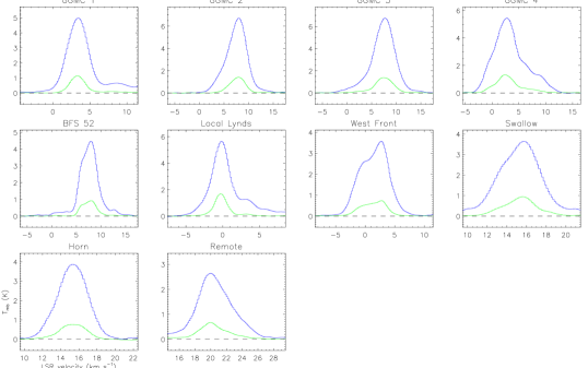
Figure 1: Mean spectra of the 10 sub-regions. Blue is ¹²CO and green is ¹³CO. The regions that contribute to the mean spectra are those where the ¹³CO emission is larger than 3$\times$RMS.

4 Data Analysis and Result

4.1 Outflow Identification

We conducted a large-scale molecular outflow survey of GOS, based on a set of semi-automated IDL scripts. we searched for and identified outflows using three-dimensional ¹²CO data (based on the longitude-latitude-velocity space), and traced the cores found in the three-dimensional ¹³CO data. We searched for the minimum velocity extents from the velocity characteristics of the three-dimensional contour diagram, conducted line diagnoses of positions with the minimum velocity extents, and finally obtained the outflow candidate samples in different quality level. The specific method is presented in Appendix A. Table 2 shows the results of the first five outflow candidates in GGMC 2. The details of each outflow candidate in each sub-region are shown Appendix C (table). We did not include outflow candidates with quality level D in Table 2 and Appendix C, because they were removed from the final sample (see Appendix A. 6, a scoring system with quality level A-D was introduced to classify all outflow candidates, where A denoted the most likely outflow candidates, and D denoted the abandoned outflow candidates).

Table 2: Examples of Outflow candidates in GGMC 2

Index	$l$	$b$	Blue Line Wing	Red Line Wing	Quality level	WISE Emission	New Detection
	(°)	(°)	(km s-1)	(km s-1)	Blue$|$Red
G2-1	192.455	0.005	$(1.2,3.5)$	$\cdots$	B	Y?	Y
G2-2	192.580	0.210	$\cdots$	$(10.2,12.4)$	B	Y?	Y
G2-3	192.598	-0.048	$(-0.2,4.3)$	$(11.0,15.9)$	A$|$A	Y	N
G2-4	192.608	-0.129	$(0.5,4.3)$	$\cdots$	C	Y?	Y
G2-5	192.655	-0.210	$\cdots$	$(11.0,13.0)$	A	Y?	Y

Note. — Y = Yes, Y? = possible, N = Not a new detection. The quality level see Appendix A. 6. Since the outflow candidates with score D were removed from the final sample, we do not include them in this table.

Table 3 summarizes the outflow survey results where outflow candidates with quality level D are not included. 134 outflow candidates are located in Gem OB1 which is located in the Perseus arm, 96% being newly detected. Twenty-one detected outflow candidates are associated with the Local arm, which includes Local Lynds and West Front. Forty-three outflow candidates were detected beyond the Perseus arm.

Table 3: Outflow candidate Sample Statistics

Sub-region	Numbers of Outflow	Numbers of	Quality Level
	Total(Blue$|$Red)	Bipolar Outflow	A	B	C
GGMC 1	34(22$|$18)	6	3$|$8%	19$|$48%	18$|$45%
GGMC 2	20(11$|$16)	7	7$|$26%	13$|$48%	7$|$26%
BFS 52	17(12$|$13)	8	8$|$32%	10$|$40%	7$|$28%
GGMC 3	45(28$|$31)	14	25$|$42%	28$|$47%	6$|$10%
GGMC 4	18(13$|$8)	3	8$|$38%	8$|$38%	5$|$24%
Local Lynds	2(2$|$1)	1	1$|$33%	2$|$67%	0$|$0%
West Front	19(13$|$11)	5	1$|$4%	13$|$54%	10$|$42%
Swallow	10(5$|$7)	2	4$|$33%	7$|$58%	1$|$8%
Horn	9(8$|$9)	8	7$|$41%	8$|$47%	2$|$12%
Remote	24(17$|$16)	9	9$|$27%	15$|$45%	9$|$27%
Total	198(131$|$130)	63	73$|$28%	123$|$47%	65$|$25%

Note. — In “Quality Level” column, we presented the numbers and percentages and separated them with a “$|$”. The definition of quality level see Appendix A. 6.

There are six previously known outflows in GOS. Five of them are included in the detected outflow candidates, the other which are associated with CB39 (Yun & Clemens, 1992; Wang et al., 1995) was manually removed from the outflow sample, because of the quality level (see Figure A. 4, and Appendix A. 6). The two works shared a similar HPBW ($\sim 48\arcsec$) and sensitivity (0.25 K per 250 kHz channel, corresponding to a velocity resolution of 0.65 km s^-1 at 115 GHz) to this work. However, they did not show an image of the outflow, we were unable to figure out the reason why this one was failed to be detected.

4.2 The Limitation of the Survey

Although we found a large number of outflow candidates, some with faint emission, low velocity, complex environment or small size could be missed. In addition, owing to the moderate resolution, the identified outflow candidates, especially for those at large distances, can in fact be multi-outflows. We reported specifically the limitation of this survey from three aspects in the following. First, the sensitivity is 0.45 K per 61 kHz channel (corresponding to $\sim$ 0.16 km s^-1 at 115.271 GHz) for ¹²CO, some fainter or low-velocity outflows could be missed. Second, the interaction between outflows and ambient gas at large scales makes their morphologies uncertain, which would present confused morphologies in the maps. Therefore, many outflow candidates detected with one lobe (either red or blue) does not indicate that they are genuine monopolars. Their counterflows can be too faint/confused to be detected.

Last and most important, owing to moderate resolution, small size outflows ($\lesssim$ 49$\arcsec$) cannot be detected, and the identified outflow candidates could be multi-outflows. Two CO (1-0) outflows surveys with the similar HPBW ($\sim$ 46$\arcsec$) were selected to estimate the possible multi-outflows. The two outflow surveys were toward Perseus and Taurus molecular clouds (hereafter PTC, Arce et al., 2010; Li et al., 2015). The mean outflow radius in PTC were $\sim$ 0.5 and $\sim$ 0.3 pc (Arce et al., 2010; Li et al., 2015), corresponding to $\gtrsim 154\arcsec$ and $\gtrsim 103\arcsec$ at 400–600 pc, respectively. These angular sizes are greatly larger than the HPBW of the current study ($\sim$ 49$\arcsec$), indicating that most outflow candidates in Local Lynds and West Front are resolvable. The mean angular outflows size in PTC corresponded to $\sim$ 31$\arcsec$ and $\sim$ 52$\arcsec$ at 2 kpc, respectively. These angular sizes are close to the HPBW, which indicates that some outflow candidates in Gem OB1 are bulk outflow candidates. Therefore, we expected a bias towards higher values of the derived quantities but lower detection rates. However, the mean angular outflows size in PTC corresponded to $\lesssim$ 22$\arcsec$ at $\geq$ 3.8 kpc, which is significantly less than the HPBW. Outflow candidates were highly clumpy in regions with distance $\geq$ 3.8 kpc.

What is more, the distances in Swallow, Horn or Remote are undetermined, see Paper I. To avoid the great uncertainties in physical parameters toward these three sub-regions, we did not investigate the outflow candidates’ properties and only studied the spatial distribution of outflow candidates in these regions in the following contents, see Section 5.1. The reserved information, especially the positions and line wing velocity ranges of outflow candidates presented in Appendix C (table), will contribute to future high-resolution investigations.

As a pilot outflow survey, this study probably underestimates outflow impact by mis-identifying outflow candidates. Higher resolution observations would be followed up to identify individual outflows.

4.3 The Amount of Possible Outflow Emission Missed

Outflows column density, $N_{\mathrm{o}}$, i.e., the number of outflows per square pc, can indicate the level of undetected outflows. Because YSO column density, $N_{\mathrm{Y}}$, in PTC ($\sim$ 1.3 pc^-2, Evans et al., 2009; Arce et al., 2010; Rebull et al., 2010) is slightly higher than that in the part of Gem OB1 that surrounds SH 252 (i.e., 0.5 pc^-2, Jose et al., 2012, 2013), indicating that star formation in Gem OB1 is less active than that in PTC. We therefore expected a smaller $N_{\mathrm{o}}$ in Gem OB1 (located in the Perseus arm) and the Local arm, where star formation in the Local arm is generally less active than that in the Perseus arm. Arce et al. (2010) and Li et al. (2015) found $N_{\mathrm{o}}\approx$ 0.2 pc^-2 in PTC. Given the same distance ($\sim$ 2 kpc) and a similar $N_{\mathrm{Y}}$ (0.6 pc^-2, Koenig et al., 2008) to Gem OB1, Ginsburg et al. (2011) only found 40 CO (2-1) outflows in W5 within $\sim$ 4060 pc², where the HPBW ($\sim$ 14$\arcsec$) and sensitivity (0.1 K per 0.4 km s^-1 channel) were superior to the current study. Combining the surveys in PTC and in W5, the actual number of outflows should be greater than the detected count by factors of no more than 16, 10, 8, 13, 11, 3, and 13 (i.e., scale-up factors, SUFs) for the first seven sub-regions in Table 1, respectively.

4.4 Physical Parameters

The estimated physical parameters included candidate outflow lobe velocity ($\langle\Delta v_{\mathrm{lobe}}\rangle$), length ($l_{\mathrm{lobe}}$), mass ($M_{\mathrm{lobe}}$), momentum ($P_{\mathrm{lobe}}$), kinetic energy ($E_{\mathrm{lobe}}$), dynamical timescale ($t_{\mathrm{lobe}}$), and luminosity ($L_{\mathrm{lobe}}$). The calculations were described in Appendix B. As an example, Table 4 lists the physical properties of the first five outflow candidates in GGMC 2, and the complete sample are cataloged in Appendix D (for the definition of the location of outflow candidates, see Appendix A. 5.).

Table 4: Physical Properties of the Outflow Candidate Samples

Index	Lobe	$l$	$b$	$\langle\Delta v_{\mathrm{lobe}}\rangle$	$l_{\mathrm{lobe}}$	$M_{\mathrm{lobe}}$	$P_{\mathrm{lobe}}$	$E_{\mathrm{lobe}}$	$t_{\mathrm{lobe}}$	$L_{\mathrm{lobe}}$
		($\arcdeg$)	($\arcdeg$)	(km s-1)	(pc)	(M⊙)	(M⊙ km s-1)	(1043 erg)	(105 yr)	(1030 erg s-1)
G2-1	Blue	192.455	0.005	3.0	2.75	0.99	2.99	8.97	6.8	4.2
G2-2	Red	192.580	0.210	1.9	1.34	0.65	1.24	2.32	4.1	1.8
G2-3	Blue	192.604	-0.054	5.4	1.49	1.19	6.44	34.50	2.0	53.9
	Red	192.589	-0.042	5.6	2.10	3.97	22.30	124.00	2.4	164.0
G2-4	Blue	192.608	-0.129	4.8	1.49	0.92	4.39	20.80	2.4	28.4
G2-5	Red	192.655	-0.210	4.2	1.83	0.84	3.53	14.70	3.4	14.1

Three major issues can affect the uncertainties of the derived outflow parameters, namely, inclination, blending, and opacity (Arce & Goodman, 2001b). The inclination is the angle between the long axis of the outflow and the line of sight. Assuming a random distribution of inclination angles, the mean value is given by $\langle\theta\rangle=\int^{\pi/2}_{0}\theta\sin\theta d\theta=57\arcdeg.3$ (Bontemps et al., 1996; Dunham et al., 2014). Then, the velocity, length, and dynamical timescale should be multiplied by a factor of about 1.9, 1.2, and 0.6, respectively. When we considered that some low-velocity outflowing gas blend into ambient gas, the outflow mass should be scaled up by a factor of $\sim$2.0, as previous studies have shown (Margulis & Lada, 1985; Arce et al., 2010; Narayanan et al., 2012). Caution was taken that those corrections were only applied to statistics. We did not estimate the correction for optical depth, which was discussed in Appendix B. Table 5 summarizes the correction factors, which also include corrections for outflow momentum, kinetic energy and luminosity. The following discussions is based on the physical parameters after correcting for inclination and blending. Table 6 shows the global physical properties (after correction) of outflow candidates in each sub-region.

Table 5: Correction Factors

Quantity	Inclination	Inclination	Blending	Total
	Dependence	Correction	Correction	Correction
$\langle\Delta v_{\mathrm{lobe}}\rangle$	1/$\cos\theta$	1.9	$\cdots$	1.9
$l_{\mathrm{lobe}}$	1/$\sin\theta$	1.2	$\cdots$	1.2
$M_{\mathrm{lobe}}$	$\cdots$	$\cdots$	2.0	2.0
$P_{\mathrm{lobe}}$	1/$\cos\theta$	1.9	2.0	3.8
$E_{\mathrm{lobe}}$	1/$\cos^{2}\theta$	3.4	2.0	6.8
$t_{\mathrm{lobe}}$	$\cos\theta/\sin\theta$	0.6	$\cdots$	0.6
$L_{\mathrm{lobe}}$	$\sin\theta/\cos^{3}\theta$	5.3	2.0	10.6

Note. — The physical quantities include outflow lobe’s velocity ($\langle\Delta v_{\mathrm{lobe}}\rangle$), length ($l_{\mathrm{lobe}}$), mass ($M_{\mathrm{lobe}}$), momentum ($P_{\mathrm{lobe}}$), kinetic energy ($E_{\mathrm{lobe}}$), the dynamical timescale ($t_{\mathrm{lobe}}$), and luminosity ($L_{\mathrm{lobe}}$).

Table 6: Global Outflow Candidate Properties (corrected) in Each Sub-region

Sub-region	Velocity	Mass	Momentum	Kinetic Energy	Luminosity	Dynamical Timescale
	(km s-1)	(M⊙)	(M⊙ km s-1)	(1044 erg)	(1032 erg s-1)	(105 yr)
GGMC 1	4.6	66.8	308.6	139.4	11.9	3.9
GGMC 2	6.5	108.6	608.2	457.6	69.2	3.2
BFS 52	3.9	34.8	144.4	61.2	6.0	3.9
GGMC 3	6.8	184.8	1394.6	1122.0	159.5	2.8
GGMC 4	7.2	48.6	471.2	474.6	113.0	2.8
Local Lynds	6.0	0.2	1.1	0.7	0.8	0.7
West Front	5.8	4.8	28.5	18.4	6.7	1.1

Note. — The physical parameter in the second and last column is the mean value of all lobes within each sub-region.

5 Discussion

5.1 The Spatial Distribution of Outflow candidates

Figures 2–11 map the outflow candidate distributions for the 10 sub-regions in Table 1 in order, and HII regions are marked. Then we inspected the locations of outflow candidates by eye in the context of ¹³CO gas emission.

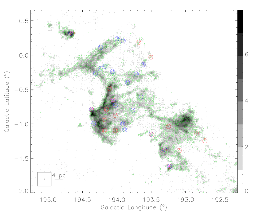
Figure 2: Outflow candidate distribution in GGMC 1. The background gray-scale map and contours are the integrated intensity map of ¹³CO in the range of [2, 9] km s^-1, and the color bar is in units of K km s^-1. The contours start at 5$\sigma$ with $\sigma=0.27$ K km s^-1, and the contour interval is 20% of the difference between the peak intensity and 5$\sigma$. The blue and red open circles denote the blue and red lobes, respectively. The blue/red numbers in the circles are the indexes of blue/red lobes, and the magenta numbers mark the bipolar outflow candidates. The definition of the location of outflow candidates refers to Appendix A. 5. The beam of the ¹³CO observations (the open circle in the insert) and physical scale bar are reported in the bottom left of the panel.

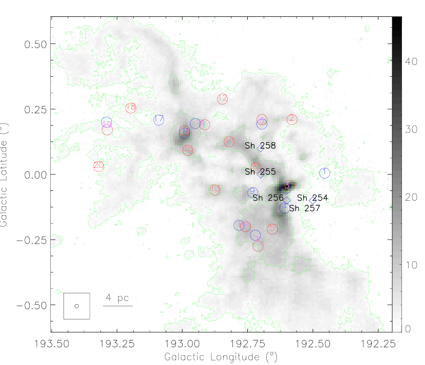
Figure 3: Outflow candidate distribution in GGMC 2. The background gray-scale map and contours are the integrated intensity map of ¹³CO in the range of [5, 11] km s^-1, and the color bar is in units of K km s^-1. The contour levels are 5, 30, 60, 90 120 $\times$ 0.25 K km s^-1 (1$\sigma$). The blue and red open circles denote the blue and red lobes, respectively. The blue/red numbers in the circles are the indexes of blue/red lobes, and the magenta numbers mark the bipolar outflow candidates. The definition of the location of outflow candidates refers to Appendix A. 5. Diamonds represent HII regions Sh 254–258 (Sharpless, 1959). The beam of the ¹³CO observations (the open circle in the insert) and physical scale bar are reported in the bottom left of the panel.

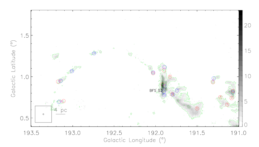
Figure 4: Outflow candidate distribution in BFS 52. The background gray-scale map and contours are the integrated intensity map of ¹³CO in the range of [5, 11] km s^-1, and the color bar is in units of K km s^-1. The contours start at 5$\sigma$ with $\sigma=0.25$ K km s^-1, and the contour interval is 20% of the difference between the peak intensity and 5$\sigma$. The blue and red open circles denote the blue and red lobes, respectively. The blue/red numbers in the circles are the indexes of blue/red lobes, and the magenta numbers mark the bipolar outflow candidates. The definition of the location of outflow candidates refers to Appendix A. 5. Diamond represents HII region BFS 52 (Blitz et al., 1982; Carpenter et al., 1995b). The beam of the ¹³CO observations (the open circle in the insert) and physical scale bar are reported in the bottom left of the panel.

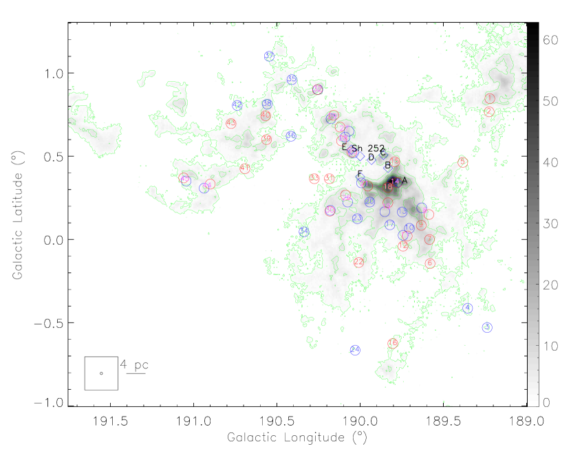
Figure 5: Outflow candidate distribution in GGMC 3. The background gray-scale map and contours are the integrated intensity map of ¹³CO in the range of [5, 11] km s^-1, and the color bar is in units of K km s^-1. The contour levels are 5, 20, 60, 100, 140 $\times$ 0.25 K km s^-1 (1$\sigma$). The blue and red open circles denote the blue and red lobes, respectively. The blue/red numbers in the circles are the indexes of blue/red lobes, and the magenta numbers mark the bipolar outflow candidates. The definition of the location of outflow candidates refers to Appendix A. 5. Diamonds represent HII regions Sh 252 (Sharpless, 1959), and A, B, C, D, E, F in Felli et al. (1977). The beam of the ¹³CO observations (the open circle in the insert) and physical scale bar are reported in the bottom left of the panel.

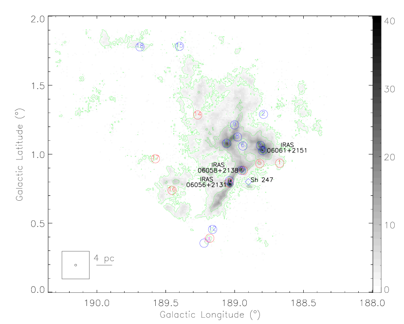
Figure 6: Outflow candidate distribution in GGMC 4. The background gray-scale map and contours are the integrated intensity map of ¹³CO in the range of [-3, 5] km s^-1, and the color bar is in units of K km s^-1. The contour levels are 5, 20, 60, 100, 140 $\times$ 0.29 K km s^-1 (1$\sigma$). The blue and red open circles denote the blue and red lobes, respectively. The blue/red numbers in the circles are the indexes of blue/red lobes, and the magenta numbers mark the bipolar outflow candidates. The definition of the location of outflow candidates refers to Appendix A. 5. Diamonds represent HII regions Sh 247 (Sharpless, 1959), and another three compact HII regions (IRAS 06051+2151, IRAS 06058+2138 and IRAS 06065+2131 in Ghosh et al., 2000). The beam of the ¹³CO observations (the open circle in the insert) and physical scale bar are reported in the bottom left of the panel.

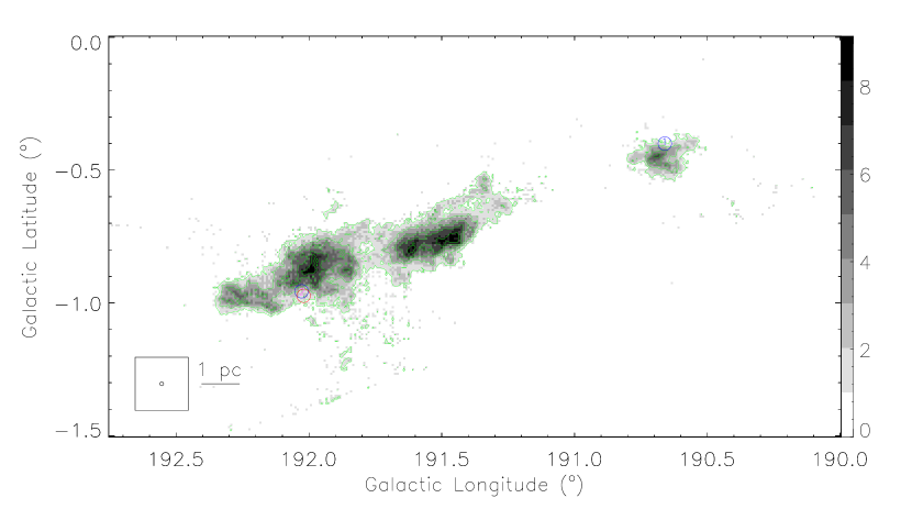
Figure 7: Outflow candidate distribution in Local Lynds. The background gray-scale map and contours are the integrated intensity map of ¹³CO in the range of [5, 11] km s^-1, and the color bar is in units of K km s^-1. The contours start at 5$\sigma$ with $\sigma=0.25$ K km s^-1, and the contour interval is 20% of the difference between the peak intensity and 5$\sigma$. The blue and red open circles denote the blue and red lobes, respectively. The blue/red numbers in the circles are the indexes of blue/red lobes, and the magenta numbers mark the bipolar outflow candidates. The definition of the location of outflow candidates refers to Appendix A. 5. The beam of the ¹³CO observations (the open circle in the insert) and physical scale bar are reported in the bottom left of the panel.

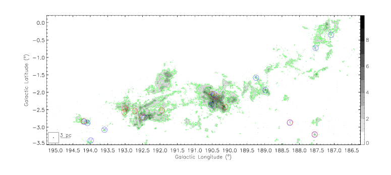
Figure 8: Outflow candidate distribution in West Front. The background gray-scale map and contours are the integrated intensity map of ¹³CO in the range of [-1, 4] km s^-1, and the color bar is in units of K km s^-1. The contours start at 5$\sigma$ with $\sigma=0.23$ K km s^-1, and the contour interval is 20% of the difference between the peak intensity and 5$\sigma$. The blue and red open circles denote the blue and red lobes, respectively. The blue/red numbers in the circles are the indexes of blue/red lobes, and the magenta numbers mark the bipolar outflow candidates. The definition of the location of outflow candidates refers to Appendix A. 5. The beam of the ¹³CO observations (the open circle in the insert) and physical scale bar are reported in the bottom left of the panel.

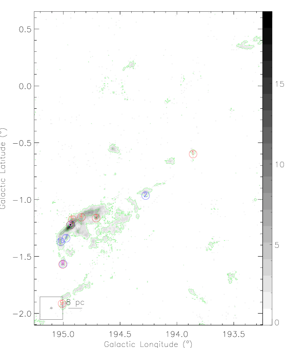
Figure 9: Outflow candidate distribution in Swallow. The background gray-scale map and contours are the integrated intensity map of ¹³CO in the range of [5, 11] km s^-1, and the color bar is in units of K km s^-1. The contours start at 5$\sigma$ with $\sigma=0.25$ K km s^-1, and the contour interval is 20% of the difference between the peak intensity and 5$\sigma$. The blue and red open circles denote the blue and red lobes, respectively. The blue/red numbers in the circles are the indexes of blue/red lobes, and the magenta numbers mark the bipolar outflow candidates. The definition of the location of outflow candidates refers to Appendix A. 5. The beam of the ¹³CO observations (the open circle in the insert) and physical scale bar are reported in the bottom left of the panel.

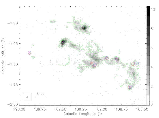
Figure 10: Outflow candidate distribution in Horn. The background gray-scale map and contours are the integrated intensity map of ¹³CO in the range of [12, 18] km s^-1, and the color bar is in units of K km s^-1. The contours start at 5$\sigma$ with $\sigma=0.25$ K km s^-1, and the contour interval is 20% of the difference between the peak intensity and 5$\sigma$. The blue and red open circles denote the blue and red lobes, respectively. The blue/red numbers in the circles are the indexes of blue/red lobes, and the magenta numbers mark the bipolar outflow candidates. The definition of the location of outflow candidates refers to Appendix A. 5. The beam of the ¹³CO observations (the open circle in the insert) and physical scale bar are reported in the bottom left of the panel.

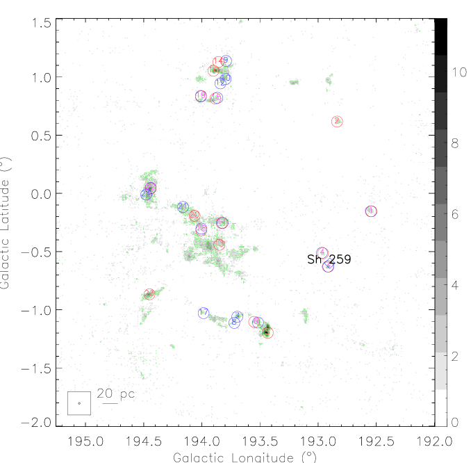
Figure 11: Outflow candidate distribution in Remote. The background gray-scale map and contours are the integrated intensity map of ¹³CO in the range of [18, 28] km s^-1, and the color bar is in units of K km s^-1. The contours start at 5$\sigma$ with $\sigma=0.33$ K km s^-1, and the contour interval is 20% of the difference between the peak intensity and 5$\sigma$. The blue and red open circles denote the blue and red lobes, respectively. The blue/red numbers in the circles are the indexes of blue/red lobes, and the magenta numbers mark the bipolar outflow candidates. The definition of the location of outflow candidates refers to Appendix A. 5. Diamond represents HII region Sh 259 (Sharpless, 1959). The beam of the ¹³CO observations (the open circle in the insert) and physical scale bar are reported in the bottom left of the panel.

Generally, outflow candidates in GGMC 1 (Figure 2), BFS 52 (Figure 4) and Swallow (Figure 9) are mainly associated with ¹³CO intensity peaks, and are preferentially located at ring-like or filamentary structures (see Paper I figures, marked by “A” and “F”, respectively). However, outflow candidates are ubiquitously distributed in GGMC 2 (Figure 3), GGMC 3 (Figure 5), GGMC 4 (Figure 6), Local Lynds (Figure 7), West Front (Figure 8), Horn (Figure 10) and Remote (Figure 11).

Table 7 summarizes the strong outflow candidates (who simultaneously have the top 25% values in each sub-region in velocity, momentum, energy, and luminosity) and their distributions. To better describe the outflow candidates distributions, we classified them into four groups as follows: group I is located in filamentary or ring-like structures; group II is close to ¹³CO intensity peaks (its distance from the local highest contour boundary is no more than 3$\arcmin$); group III is close to HII regions (the nearest HII regions is no more than 5$\arcmin$ away); group IV is deviated from the ¹³CO intensity peaks (opposite to group II). We did not consider outflow candidates in Local Lynds because there were only two outflow candidates in this region, or in Swallow, Horn or Remote, because their physical parameters were not calculated. Some strong outflow candidates in group I, and most of them are associated with ¹³CO intensity peaks (group II). The majority of the strong outflow candidates are in group II, and most of them are close to HII regions (group III) indicating that star formation was somewhat relative with HII regions. However, a few strong outflow candidates deviated from the ¹³CO intensity peaks (group IV).

Table 7: The Strong Outflow Candidates and Their Distributions

Sub-region	Amount	Indexes	Group I	Group II	Group III	Group IV
GGMC 1	3	G1-21, G1-22 G1-29	$\cdots$	G1-21	$\cdots$	G1-22, G1-29
GGMC 2	1	G2-3	$\cdots$	G2-3	G2-3	$\cdots$
BFS 52	2	B-3, B-12	B-3, B-12	B-3, B-12	B-12	$\cdots$
GGMC 3	4	G3-14, G3-17, G3-18, G3-21	$\cdots$	G3-14, G3-18, G3-21	G3-14, G3-18, G3-21	G3-17
GGMC 4	3	G4-7, G4-8, G4-10	G4-10	G4-7, G4-10	G4-7, G4-10	G4-8
West Front	2	W-7, W-9	$\cdots$	W-7	W-9	$\cdots$
Total	15	$\cdots$	$\cdots$	$\cdots$	$\cdots$	$\cdots$

5.2 Feedback of Outflow Candidates

In this section, we will discuss the feedback from outflow candidates. Table 8 shows the physical properties of each sub-region. Most clouds in Gem OB1, including GGMC 2, BFS 52, GGMC 3, GGMC 4, are massive star formation regions (Paper I). For massive molecular outflows, although the derived physical parameters include contributions from multi-outflows, they are most likely dominated by one massive flow (Beuther et al., 2002b; Tan & McKee, 2002). It is possible that, in most cases, the discovered outflow candidates are clustered outflow candidate systems as shown in Beuther et al. (2002b) and Tan & McKee (2002). We neglect the effects due to multiple sources in the following. Future high resolution study will be of great interest.

5.2.1 Impact of Outflow Candidates—Energy

We analyzed the impact of the total energy of outflow candidates on the whole cloud. The turbulent energy of the cloud is given by (Arce et al., 2010):

$$E_{\mathrm{turb}}=0.5M_{\mathrm{cloud}}\sigma^{2}_{\mathrm{3d}},$$ (1)

where $M_{\mathrm{cloud}}$ is the total mass of the cloud (see Paper I or Table 8). $\sigma_{\mathrm{3d}}=\sqrt{3}\Delta V/2\sqrt{2\ln 2}$, where $\Delta V$ is the line width of the mean ¹³CO spectrum of each sub-region (see Table 8).

Table 8: Global Physical Properties of the Sub-regions

Sub-region	$M_{\mathrm{cloud}}$	$R_{\mathrm{cloud}}$	$\Delta V$	$T$	$E_{\mathrm{turb}}$	$t_{\mathrm{ff}}$	$t_{\mathrm{diss}}$	$L_{\mathrm{turb}}$	$v_{\mathrm{esc}}$	$E_{\mathrm{grav}}$
	($10^{3}$ M⊙)	(pc)	(km s-1)	(K)	(erg)	($10^{6}$ yr)	($10^{6}$ yr)	(erg s-1)	(km s-1)	(erg)
GGMC 1	36	32	2.4	8.3	1.1E+48	15.8	6.9	5.1E+34	3.1	3.5E+48
GGMC 2	60	21	3.5	10.2	4.0E+48	6.5	4.9	2.6E+35	5.0	1.5E+49
BFS 52	14	21	3.5	7.8	9.2E+47	13.5	4.2	7.1E+34	2.4	8.0E+47
GGMC 3	110	27	4.0	10.2	9.5E+48	7.0	4.2	7.1E+35	5.9	3.8E+49
GGMC 4	55	21	4.2	8.8	5.2E+48	6.8	3.5	4.8E+35	4.7	1.2E+49
Local Lynds	1	4	1.9	9.2	1.9E+46	4.2	1.8	3.4E+33	1.5	2.1E+46
West Front	8	22	6.4	6.9	1.8E+48	19.1	0.8	6.5E+35	1.8	2.5E+47

Table 9: The Impact of outflow candidates (Corrected) on its Parent Cloud

Cloud	$E_{\mathrm{flow}}/E_{\mathrm{turb}}$	$L_{\mathrm{flow}}/L_{\mathrm{turb}}$	$E_{\mathrm{flow}}/E_{\mathrm{grav}}$	$M_{\mathrm{esc}}/$M⊙	$M_{\mathrm{esc}}/M_{\mathrm{flow}}$	$M_{\mathrm{esc}}/M_{\mathrm{cloud}}$
GGMC 1	1.2E-02	2.4E-02	4.0E-03	99	1.5	2.8E-03
GGMC 2	1.2E-02	2.8E-02	3.1E-03	137	1.3	2.3E-03
BFS 52	6.4E-03	8.5E-03	7.4E-03	60	1.8	4.3E-03
GGMC 3	1.2E-02	2.2E-02	2.9E-03	236	1.3	2.1E-03
GGMC 4	9.1E-03	2.4E-02	3.8E-03	99	2.0	1.8E-03
Local Lynds	3.2E-03	1.2E-02	2.9E-03	1	3.5	7.8E-04
West Front	1.0E-03	1.0E-03	7.4E-03	16	3.3	2.0E-03

Comparing Table 6 with Table 8 regions by regions, the total kinetic energy of these detected outflow candidates in each sub-region is much less than the total turbulent energy of the corresponding cloud, and ratio of the two parameters in each sub-region is $\leq$ 1.2% (see Table 9). The maximum $E_{\mathrm{flow}}/E_{\mathrm{turb}}=$ 19% when we considered the SUFs. This indicates that outflows cannot provide enough energy to balance the turbulent energy in each sub-region at the scale of the whole cloud. Therefore, there must be some other sources of energy that support the turbulence, such as expanding shells, stellar winds, and gravity-driven turbulence (Arce et al., 2011; Krumholz & Burkhart, 2016).

Brunt et al. (2009) showed that outflows can be important on small scales using principal component analysis on CO line maps. They found that the scale of the regions influenced by small scale driving by outflows was $\sim$ 0.3–0.6 pc in NGC 1333, assuming a distance of 235 pc (Hirota et al., 2008). Combined the ¹²CO and ¹³CO (1-0) data from the FCRAO (single dish) and CARMA (interferometry) observations, Plunkett et al. (2013) suggested that outflows are likely important agents to maintain the turbulence in this region at a scale of $\sim$ 0.5 pc. Specifically, $E_{\mathrm{flow}}/E_{\mathrm{turb}}\sim$ 35%, $L_{\mathrm{flow}}/L_{\mathrm{turb}}\sim 20$, $E_{\mathrm{flow}}/E_{\mathrm{grav}}\sim$ 1.4, where the definitions of the last two terms see Sections 5.2.2 and 5.2.3, respectively. Other studies, such as Fuller & Ladd (2002), Arce & Sargent (2006) and Arce et al. (2010), have also shown that outflows have significant impact on their environments within few parsecs. The cloud scale in current study (several pc to dozens of pc) is too large. That could be the main reason why outflows are insufficient to provide required power to maintain turbulence.

5.2.2 Impact of Outflow Candidates—Luminosity

To estimate the impact of outflow candidates on the surrounding environment, another important way is to compare the total energy injection rate of outflow candidates (the total luminosity of outflow candidates) with the turbulence luminosity (the turbulent dissipation rate $L_{\mathrm{turb}}$) of the clouds. As mentioned above, the luminosity of a single candidate outflow lobe is $L_{\mathrm{lobe}}=E_{\mathrm{lobe}}/t_{\mathrm{lobe}}$, and the total luminosity in each sub-region is the sum of all lobe candidates located within the corresponding sub-region.

The turbulent dissipation rate $L_{\mathrm{turb}}$ is given by

$$L_{\mathrm{turb}}=\frac{E_{\mathrm{turb}}}{t_{\mathrm{diss}}},$$ (2)

where $t_{\mathrm{diss}}$ is the turbulent dissipation timescale. The numerical study of Mac Low (1999) suggested that $t_{\mathrm{diss}}$ of the energy dissipation of uniformly driven magnetohydrodynamic turbulence is approximately given by:

$$t_{\mathrm{diss}}=\left(\frac{3.9\kappa}{M_{\mathrm{rms}}}\right)t_{\mathrm{ff}},$$ (3)

where $\kappa$ is the ratio of the driving wavelength over the Jean’s length of the cloud $\lambda_{\mathrm{J}}$. $t_{\mathrm{ff}}$ is the free-fall timescale, and $M_{\mathrm{rms}}$ is the Mach number in the turbulence.

In simulations the turbulence driving length of a continuous outflow is approximately equal to the outflow lobe (see Nakamura & Li, 2007; Cunningham et al., 2009), therefore the driving wavelength is set to be the mean outflow candidate length $\lambda_{\mathrm{d}}$, and

$$\kappa=\lambda_{\mathrm{d}}/\lambda_{\mathrm{J}}.$$ (4)

The Jean’s length of the cloud is defined as

$$\lambda_{\mathrm{J}}=c_{\mathrm{s}}\sqrt{\pi/G\rho_{\mathrm{reg}}},$$ (5)

where $G$ is the gravitational constant, $c_{\mathrm{s}}$ is the sound speed and $\rho_{\mathrm{reg}}$ is the mass density of the specific cloud. For an ideal gas, $c_{\mathrm{s}}$ reads (Mac Low, 1999)

$$c_{\mathrm{s}}=(3kT/m_{H}\mu)^{1/2},$$ (6)

where $T$ is the average excitation temperature of a specific cloud (see Table 8), $k$ is the Boltzmann’s constant, $m_{H}$ is the mass of atomic hydrogen, and $\mu=2.72$ is the mean molecular weight (Brunt, 2010). $\rho_{\mathrm{reg}}$ reads

$$\rho_{\mathrm{reg}}=3M_{\mathrm{cloud}}/\left(4\pi R^{3}_{\mathrm{cloud}}\right).$$ (7)

$M_{\mathrm{cloud}}$ and $R_{\mathrm{cloud}}$ are the mass and radius of the specific cloud (see Table 8). Finally,

$$t_{\mathrm{ff}}=\sqrt{3\pi/32G\rho_{\mathrm{reg}}},$$ (8)

and

$$M_{\mathrm{rms}}=\sigma_{\mathrm{3d}}/c_{\mathrm{s}}.$$ (9)

$\sigma_{\mathrm{3d}}$ see Section 5.2.1.

Using the formulas from (2) to (9), we determined the turbulent dissipation timescale and turbulent dissipation rate of the clouds (see Table 8). Table 9 shows that the outflow candidate total luminosity is much less than the turbulent dissipation rate of the clouds suggesting that the observed outflow activity is not enough to support the measured turbulence in each sub-region, even if we considered the SUFs (the maximum $L_{\mathrm{flow}}/L_{\mathrm{turb}}$ becomes 38%). The above estimation is not flawless. The major uncertainty of $L_{\mathrm{flow}}/L_{\mathrm{turb}}$ result from the uncertainties in the outflow candidate length and dynamical timescale.

As discussed in Section 5.2.1, the main reason why outflow candidates were insufficient to provide the required power to maintain turbulence may be that the cloud scales in the study were too large.

5.2.3 Disruption of the Parent Cloud by Outflow Candidates

The study of Arce & Goodman (2002) shows that outflows can have a disruptive impact on their parent clouds, which can be evaluated by comparing the outflow energy with cloud gravitational binding energy ($E_{\mathrm{grav}}$), where

$$E_{\mathrm{grav}}=\frac{GM^{2}_{\mathrm{cloud}}}{R_{\mathrm{cloud}}}.$$ (10)

The gravitational binding energy of each cloud is listed in Table 8. Table 9 shows that the outflow candidate’s total kinetic energy in each cloud occupies just a small fraction of cloud’s gravitational binding energy (ranges from 0.3% to 0.7%), which indicates that outflow candidates cannot provide enough power to disrupt its parent cloud. The maximum $E_{\mathrm{flow}}/E_{\mathrm{grav}}$ only rises to 6% if we considered the SUFs.

Another method to judge the importance of the disruptive effect of outflow candidates on clouds is using the “escape mass” $M_{\mathrm{esc}}$ (see details in Arce et al., 2010), which is given by

$$M_{\mathrm{esc}}=\frac{P_{\mathrm{flow}}}{v_{\mathrm{esc}}}=\frac{P_{\mathrm{flow}}}{\sqrt{2GM_{\mathrm{cloud}}/R_{\mathrm{cloud}}}}.$$ (11)

From Table 9, $M_{\mathrm{esc}}/M_{\mathrm{flow}}$ ranges from 1.3 to 3.5, which implies that the current outflow candidates have strong impacts on the environment immediately surrounding them within a small distance. However, in terms of $M_{\mathrm{esc}}/M_{\mathrm{cloud}}$, the current outflow candidate momentum could potentially disperse only $\leq$ 0.4% of the mass in their respective regions (see Table 9). The maximum $E_{\mathrm{esc}}/E_{\mathrm{cloud}}$ only rises to 5% if we considered the SUFs. All of these suggest that the current outflow candidates may disperse some gas from their parent clouds, but they do not have enough strength to make a serious impact at the scale of the whole cloud.

$E_{\mathrm{flow}}/E_{\mathrm{grav}}$ is $\sim$ 33%–65% at $\sim$ 0.2 pc scale in L1228 (Tafalla & Myers, 1997), where the uncertainty of this ratio depends on the power-law dependence of the density law (MacLaren et al., 1988). This ratio is $\sim$ 4%–40% at the $\sim$ 0.6–2.0 pc scale in sub-regions within the Perseus molecular cloud complex (Arce et al., 2010), and $\sim$ 0.3% at the $\sim$ 13.8 pc scale in the Taurus molecular cloud (Li et al., 2015). Therefore, scale is important for evaluating outflow impacts.

The scale of the interaction between the outflow candidates and clouds is of the order of dozens of pc in this study, hence it may not be suitable to discuss the impact of outflow candidates on the cores with size scales about a few tenths of a parsec. The results reported here do not rule out the possibility that outflows can be an important mechanism of mass-loss in cores (see e.g., Fuller & Ladd, 2002; Arce & Sargent, 2005, 2006).

6 Summaries and Conclusions

A large-scale survey of outflow features was conducted of the GOS (a total of 58.5 square degrees) using ¹²CO and ¹³CO molecular line maps, which are a part of MWISP.

We developed a set of semi-automated IDL scripts based on longitude-latitude-velocity (p-p-v) space to search for and evaluate outflows over a large area rapidly and efficiently. A total of 198 outflow candidates were identified, including 63 bipolar outflow candidates. Of these, 134 were located in the Perseus arm, which includes the Gem OB1, and 96% of them were newly detected. Twenty-one were located in the Local arm, which includes the Local Lynds dark clouds and West Front clouds, and the remaining outflow candidates were beyond the Perseus arm. Owing to the limited resolution, especially in regions with distances of $\gtrsim$ 3.8 kpc, many of the identified outflow candidates were probably multi-outflow candidates.

We analyzed the distribution of outflow candidates and discussed the impact of outflows on its surrounding gas. The limitation of this study could result in underestimating outflow impact by mis-identifying outflow candidates. The main summaries and conclusions are as follows:

1. Outflow candidates in GGMC 1, BFS 52 and Swallow were mainly associated with ¹³CO intensity peaks or located at ring-like or filamentary structures. However, outflow candidates were ubiquitously distributed in GGMC 2, GGMC 3, GGMC 4, Local Lynds, West Front, Horn and Remote. Strong outflow candidates were also mainly located at filamentary or ring-like structures, or close to ¹³CO intensity peaks or HII regions, but a few of them deviated from ¹³CO intensity peaks.

2. We obtained the ratio of the total outflow candidate kinetic energy to the turbulent energy of each host cloud, and the ratio of the outflow candidate luminosity (kinetic energy injection rate) to the luminosity (turbulence dissipation rate). Both of them were $\lesssim$ 3%, and rose to $\lesssim$ 38% if the undetected outflows were taken into consideration. These results showed that the identified outflow candidates cannot provide sufficient energy to balance turbulence for each sub-region, even undetected outflows were considered.

3. The two ratios—the total outflow candidate kinetic energy divided by cloud’s gravitational binding energy, and the “escape mass” (the cloud’s mass potentially dispersed by outflow candidates) divided by cloud’s mass—were both $\lesssim$ 1%, and rose to $\lesssim$ 6% if the undetected outflows were taken into consideration. The current outflow candidates may disperse some gas from their parent clouds, but did not have sufficient power to cause major disruptions to the cloud at the scale of the whole cloud, even accounting for undetected outflows.

Appendix A Outflow Identification Methodology

We conducted an unbiased, blind outflow survey toward studied region. To ensure efficiency and precision of the outflow identification, we developed a set of semi-automated IDL scripts for outflow searching. The scripts consist of seven steps. The example shown in this section is of sub-region GGMC 2.

A.1 The Distribution of ¹³CO Peak Velocity

The first step is to extract spectral data for each pixel from three-dimensional ¹³CO data of each sub-region. For each pixel, if the signal was larger than 3$\times$RMS in the velocity range, the velocity of the peak emission (peak velocity) would be extracted and a two-dimensional distribution map of ¹³CO peak velocity would be created (see e.g. Figure A. 1). Note that, if two or more extreme brightness temperatures were not be confused with each other, the corresponding number of peak velocity was extracted and corresponding velocity distribution diagram was created. However, when some signals with extreme brightness temperatures were blended, or the differences between the peak velocities was less than the minimum $1\sigma$ velocity dispersion (Gaussian fit) of each peak, we adopted the mean value of the peak velocities as the systemic velocity. All ¹²CO outflow candidates searched here had corresponding ¹³CO emission.

Figure A. 1: ¹³CO Peak-velocity in GGMC 2. The color-bar is in unit of km s^-1.

A.2 The Distribution of Extensional Velocities of Blue and Red Line Wings

Based on the first step, we then obtained the extensional velocities of the blue/red lobes of ¹²CO spectra of those pixels which had ¹³CO emission and obtained ¹³CO peak velocities. For a ¹²CO spectrum in a specific pixel, the scripts began with each ¹³CO peak velocity, and searched the velocity forward or backward until ¹²CO emission in three successive channels were less than the threshold temperature, and this cut-off velocity was regarded as the extensional velocity of red/blue line wings.

To facilitate the subsequent analysis, we used the maximum velocity minus the extensional velocity of the blue lobe of each pixel in each sub-region to obtain a distribution of relative velocities of blue line wings, which were in positive values. Similarly, the relative velocities of the red line wings obtained by subtracting the minimum velocity from the extensional velocity of the red lobe of each pixel in each sub-region.

It is worthwhile to note that three threshold temperatures were contained to calculate the weighted mean extensional velocities of the blue/red lobes with the weighted portion of 3:3:4. The three threshold temperatures were 1$\times$RMS, 2$\times$RMS and 0.2$\times$peak temperature (if it was larger than 3$\times$RMS, we adopted 3$\times$RMS). The threshold temperature of 1$\times$RMS was chosen to avoid missing some faint outflows. We then created the distribution of the extensional velocities of the blue and red lobes. Figure A. 2 shows the distribution of extensional velocities of the red lobes in GGMC 2.

A.3 The Positions of the Minimum Velocity Extents

We used the CUPID (Berry et al., 2007, part of the STARLINK software⁸) clump-finding algorithm FELLWALKER (Berry, 2015) to search for extreme points (i.e., the minimum velocity extents) from a distribution of extensional velocities of the blue and red lobes, and output their positions. The parameters setting in STARLINK CUPID FELLWALKER were based on the distance of a specific sub-region. The extensional velocity of a minimum velocity extent relative to ambient gases was set to be larger than 1 km s^-1. The preliminary positions of the blue and red lobes were obtained after we removed noise fluctuations. The positions of the red lobes in GGMC 2 are shown in Figure A. 2 as red pluses.

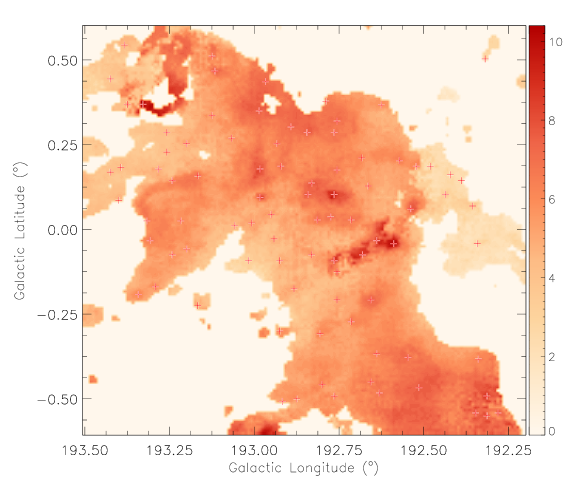
Figure A. 2: The distribution of line wing maximum velocity in GGMC 2. Red pluses mark the preliminary positions of red lobes. The color-bar is in unit of km s^-1.

A.4 Line Diagnoses of the Positions of the Minimum Velocity Extents

Inevitably, the contaminations from stellar winds and weak clouds could influence the results. Therefore, we conducted line diagnostics at every position of the minimum velocity extents, and removed outflow candidates which were obviously incompatible with the line profiles of the outflow line wings.

We preliminary estimated the velocity range of line wings in specific spectrum. The maximum line wing velocity relative to the peak velocity was the extensional velocity of the ¹²CO line wing, and the minimum one was the extensional velocity of the ¹³CO line wing or the maximum FWHM of ¹²CO. The line diagnostic criteria were as follows: first, to avoid mistaking core components as outflow components, the maximum velocity of a ¹²CO line wing relative to the peak velocity should be greater than 2 km s^-1 , and should be larger than the thermal velocity (taken as the FWHM of ¹²CO or the extensional velocity of the ¹³CO line wing). Second, to remove the interfering components along the line-of-sight, the ¹²CO profile in the velocity range of the line wing should decrease successively.

In spite of such strict criteria promote the reliability of outflow candidate samples, it could miss the outflow candidates blended with other components. To guarantee the completeness of outflow candidate samples, we slightly loosened the second criterion that the ¹²CO profile could contain non-obvious bumps which covered less than 6 channels (i.e., 1.0 km s^-1). This step obtained outflow candidate samples.

A.5 Plot Outflow Candidate’s Contours and P-V Map Diagrams

In this step, we plotted the integrated intensity map and contours over the entire line wing velocity range of the blue/red lobes for each outflow candidate, then plotted a position-velocity (P-V) diagram along four directions to investigate their velocity structure. This step was completed by eye. According to the contours and the P-V diagrams, we adjusted the line wing velocity ranges of the blue/red lobes or positions of outflow candidates to make the contours under an ideal state (i.e., make the score defined in A. 6 as high as possible). We then assigned the final position and the velocity range of outflow ling wings for each outflow candidate. Figure A. 3 and Figure A. 4 presents two examples from outflow candidates in GGMC 2 (red lobe of G2-3) and West Front (removed from our sample later), respectively. In Figure A. 3–A. 5, we arbitrarily chose $3\times 3$ pixels window to average spectra (both for ¹²CO and ¹³CO) to improve the signal-to-noise ratio of the spectra. Maps like Figure A. 3 and Figure A. 4 are the direct sources of the scoring system for outflow candidates in the next subsection.

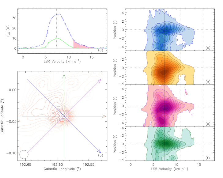
Figure A. 3: Red lobe of G2-3 in GGMC 2. (a), the blue and green spectra are the ¹²CO and ¹³CO averaged over $3\times 3$ pixels centered at the emission peak of ¹²CO red lobe, respectively; and the pink shaded part of the spectrum indicates the ¹²CO line wing velocity range. (b), red ¹²CO lobe contours, the lowest contour of the lobes is 20% of the peak intensity, the contour interval is 5% of the peak intensity, and the color lightness of the contours increase with the intensity. (c)–(f), position-velocity (P-V) diagrams along the arrows with the same colors showed in panel (b), specifically, panels (c)–(f) correspond to the blue (point to southwest), yellow (point to west), purple (point to northwest) and green (point to north) arrows in panel (b), respectively; the width to draw the P-V diagram is 1$\arcmin$ (2 pixels); the lowest contour level of the P-V diagram is 5% of the maximum value, as are the contour intervals. The open circle in the left-bottom corner indicates the size of HPBW of ¹²CO.

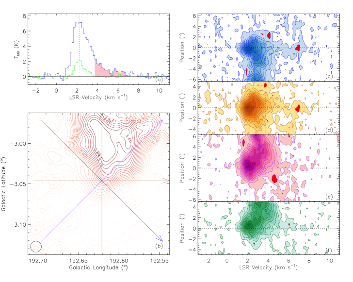
Figure A. 4: A red lobe in West Front which was removed from our sample. The description of this figure refers to Figure A. 3.

A.6 Scoring System and bipolar outflow candidates

To estimate the quality level of the outflow candidates obtained above, we set an artificial scoring system based on the line profiles, contour morphologies and P-V diagrams. Table A. 1 presents the detailed criteria. The overall score of a outflow lobe candidate calculated by adding all score of sub-items together. Table A. 2 presents the quality levels based on the overall scores.

Samples with quality levels of A are typically high-velocity outflows and the most reliable outflow candidates. Samples with quality levels of B are reliable, and the majority of outflow candidates belong to this classification. For samples with quality level C, the characteristics of the outflows are not obvious, but we cannot rule out the possibility of outflow activity in those candidates. We removed all outflow candidates with quality level D from our sample owing to their ambiguous outflow characteristics. The quality level is A for outflow candidate shown in Figure A. 3. However, for the example (associated with CB 39 in Yun & Clemens, 1992; Wang et al., 1995) shown in Figure A. 4, the quality level is D, thus being removed from our sample.

Table A. 1: Detail Criterion of Scoring System

Line Profile	P-V map	Contours	Sub-Item Score
Clear or Not	Minimum Velocity Extent	Isolate or Not (Morphology)
Clear	Obvious Bulge	Absolute Isolate	3
Non-obvious bumps	Bulge with contamination	Differentiable	2
Contamination	No bulge or chaotic	Confused with Ambient Gas	1

Note. — The four columns are the line profile of the line wings, P-V map, lobe contours, and sub-item score.

Table A. 2: Quality Level

Composite Score	Quality Level
8-9	A
6-7	B
4-5	C
3	D

In addition, blue and red lobes were paired up to form a bipolar outflow candidate if the two lobes were close (within 1.5 pc) or had similar core component structures (an example shows in Figure A. 5. of subsection A. 7). Column density of outflows (i.e., the number of outflows per square pc) was about 0.2 pc^-2 in previous studies (e.g., Arce et al., 2010; Li et al., 2015), therefore the average spatial interval of outflows was $\sim$ 4.5 pc indicating the threshold of 1.5 pc can be feasible.

Since the separation between the two lobes of R-6 is $\sim 5.1$ pc ($\sim 2\arcmin$), it is dubious to regard them as a bipolar outflow candidate. Another cases that remain to be determined include outflow candidates B-5 ($\sim 1.6$ pc apart), B-16 ($\sim 2.0$ pc apart), G3-8 ($\sim$ 2.0 pc apart), G3-11 ($\sim 1.6$ pc apart), G3-19 ($\sim 2.0$ pc apart), G3-27 ($\sim 2.0$ pc apart), G3-44 ($\sim$ 1.6 pc apart), G4-13 ($\sim 1.9$ pc apart), H-1 ($\sim 3.4$ pc apart), R-15 ($\sim 2.6$ pc apart) and R-18 ($\sim 2.1$ pc apart). We also cannot rule out the possibility that bipolar outflow candidates are several interacting outflows in some regions crowded with outflows (e.g., outflow candidates G3-21 and G3-22, etc.). Low spatial resolution of this work prevents further analysis of this problem. The total score and quality level of the bipolar outflow candidates were determined by the highest level.

A.7 Outflow Exhibition and Comparison with WISE False Color Maps

Figure A. 5 shows an example of outflow candidate G2-4 in GGMC 2. The green-filled contours in the left-bottom present the integrated intensity map of ¹³CO core components superimposed by the contours of outflow lobes (blue/red for blue/red lobe). For bipolar outflow candidates, the integral velocity range from the incipient velocity of the blue line wing (starting with the peak velocity to the left) to the incipient velocity of the red line wing (starting with peak velocity to the right). For a monopolar outflow candidate, the integral velocity range is from the incipient velocity of blue/red line wing to its symmetrical point, and the symmetry axis is the peak velocity. The number of contour levels of ¹³CO integrated intensity is 15, with a contour interval of 1/15 of the difference between the maximum and minimum integrated intensity in the mapped region. However, to sketch the contours of the main outflow candidate’s structure, the incipient value of an outflow candidate’s contour depends on the specific source, typical in the level of $\gtrsim 40$% of the maximum integrated intensity in the mapped region.

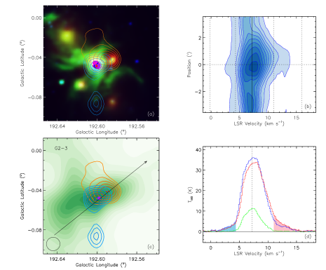
Figure A. 5: An exhibition of outflow candidate G2-3 in GGMC 2. (a): Wise 4.6 (blue), 12 (green), 22 (red) $\mu$m false color image, and blue/red lobe contours. (b): a position-velocity (P-V) diagram along the black arrow shown in panel (c); the width to draw the P-V diagram is 1$\arcmin$ (2 pixels). (c): blue/red ¹²CO lobe contours overlaid on the integrated intensity of ¹³CO cores depicted as green-filled contours. The black arrow begins from the position of a blue lobe and points to the red lobe for a bipolar outflow candidate, and for a monopolar outflow candidate the angle is 45$\arcdeg$. (d): the blue/red spectrum is the ¹²CO averaged over $3\times 3$ pixels centered at the blue/red emission peak positions, respectively; the green spectrum is the ¹³CO averaged over $3\times 3$ pixels centered at the purple point in the left-upper or left-bottom panel, which denotes the position of outflow candidate. The blue/red shaded part of the spectrum indicates the blue/red line wing velocity range of ¹²CO. The black dotted line in the center is of the peak velocity of ¹³CO. The open circle in the left-bottom corner shows the size of HPBW of ¹²CO.

Infrared source is located at/near the center of outflows (Zhang et al., 2001). The high-sensitivity mid-infrared images from the Wide-field Infrared Survey Explorer (WISE, Wright et al., 2010) indicate the protostar activity that likely drive outflows. We therefore superimposed the outflow candidate contours on the WISE image and checked by eye for a point of light in the WISE image, see an example in Figure A. 5 (a). We only considered the ¹³CO emission which associated with outflow lobe candidate (defined as ¹³CO emission whose peak is the closest to the outflow lobe candidate). If there are WISE spots within the first five contour levels of ¹³CO emission starting from the ¹³CO peak emission, the outflow candidate was regarded as having WISE associations (denote as “Y” in the column “WISE Detection” in Table C). If there are WISE spots within $30\arcsec$ (the pixel size of the current study) of the lowest contour of the ¹²CO outflow lobe, the outflow candidate was regarded as likely having WISE associations (denote as “Y?” in the column “WISE Detection” in Table C). Figure 3 in Paper I indicated that there is little overlap among these 10 sub-regions in terms of ¹³CO emission. Therefore, it is probable that the outflow candidates are associated with WISE emission (rather than happen to corresponding WISE spot lies along the line of sight). However, it is hard to rule out the possibility that the outflow candidates actually happen to coincide with a WISE spot in complicated cluster environments (e.g., Chen et al., 2016), future high resolution investigation will be of great interest.

The outflow candidates reported here are likely to have WISE associations. In most cases, ¹²CO wing emission of outflow candidates is spatially confined (i.e., has limited spatial extent, e.g., the blue/red ¹²CO lobe contours in Figure A. 5), which is an essential feature of a typical outflow (Zhang et al., 2001).

Appendix B Calculation of Outflow Candidate’s Parameters

The areas and lengths of outflow lobe candidates ($A_{\mathrm{lobe}}$ and $l_{\mathrm{lobe}}$) can be estimated by their contours. As Figure A. 5 shows, generally speaking, the area of a relatively isolated lobe candidate is decided by the 40% of peak integrated intensity. For outflow candidates which are contaminated by other components but can be resolved, we estimated the maximum areas of the vicinity of lobes where the outflow candidate components can be distinguished from other components. As a result of the limited resolution and great distance, the detailed structures of outflow candidates are usually unresolvable, so we calculated $l_{\mathrm{lobe}}$ by assuming a typical collimation factor of 2.45 (Wu et al., 2004). The outflow lobe candidate length reads $l_{\mathrm{lobe}}=1.77\sqrt{A_{\mathrm{lobe}}}$. For a bipolar outflow candidate, its area and length were estimated by averaging the area and length of its two lobes.

Similar to Beuther et al. (2002b), we adopted the line wing velocity which was the furthest away from the central systemic velocity to compute the dynamical timescale of outflow lobe candidates, see as follow:

$$t_{\mathrm{lobe}}=\frac{l_{\mathrm{lobe}}}{\Delta v_{\mathrm{max}}},$$ (B1)

where $l_{\mathrm{lobe}}$ is the outflow lobe candidate length, and $\Delta v_{\mathrm{max}}$ is the maximum outflow lobe candidate velocity. The value of $\Delta v_{\mathrm{max}}$ presented here is based on the sensitivity of our data, i.e., 0.45 K.

To estimate the mass of each lobe candidate, we computed the column density of each ¹²CO lobe line wing. Referring to Garden et al. (1990), and assuming that the excitation of all energy levels are the same, the column density of a linear, rigid rotor molecular from one transition under conditions of LTE is

$$N=\frac{3k}{8\pi^{3}B\mu^{2}}\frac{\exp[hBJ(J+1)/kT_{\mathrm{ex}}]}{J+1}\frac{T_{\mathrm{ex}}+hB/3k}{1-\exp({-h\nu/kT_{\mathrm{ex}}})}\int{\tau_{\nu}}dv,$$ (B2)

where $J$ is the quantum number of the lower rotational level, and $B$ and $\mu$ are the rotational constant and permanent dipole moment, respectively. For ¹²CO, we assume that the high-velocity gas is optically thin, and the area filling factor $f=1$, the total column density reads (see Snell et al., 1984)

$$N(^{12}\mathrm{CO})=4.2\times 10^{13}\frac{T_{\mathrm{ex}}}{\exp(-5.5/T_{\mathrm{ex}})}\int{T_{\mathrm{mb}}}dv,$$ (B3)

where the integrated range is the wing range. The excitation temperature $T_{\mathrm{ex}}$ is assumed to be 30 K. Arce & Goodman (2001a), Arce et al. (2010) used the main beam temperature in core centers to compute $T_{\mathrm{ex}}$; however, this approach would underestimate $T_{\mathrm{ex}}$ for the beam dilution effect in our moderate resolution.

Although we have ¹²CO and ¹³CO data, we did not estimate the optical depth, because in most cases ¹³CO emission is not strong enough as a signal in the velocity range of the ¹²CO line wing. Based on the assumption of optical thin ¹²CO line wing, the column density is underestimated to some extent. However, in fact, the errors of the column density arising from other factors are more significant, including: the error of the interception of outflow candidate velocity (for example, ignoring the low-velocity outflow candidate component that is blended with cores), and the error of the estimation of lobe candidate area.

The column density of H₂ gas, $N$, can be calculated by multiplying $N(^{12}\mathrm{CO})$ by a conversion factor $[\mathrm{H}]/[^{12}\mathrm{CO}]$ $=1\times 10^{4}$ (see e.g., Snell et al., 1984). The mass of the outflow lobe candidate is as follow:

$$M_{\mathrm{lobe}}=(N_{\mathrm{lobe}}\times A_{\mathrm{lobe}})m_{\mathrm{H_{2}}},$$ (B4)

where $M_{\mathrm{lobe}}$, $A_{\mathrm{lobe}}$ and $N_{\mathrm{lobe}}$ are the mass, area and column density of blue/red lobe of outflow candidates, respectively, and $m_{\mathrm{H_{2}}}$ is the mass of a hydrogen molecule. If the outflow candidate is bipolar, the mass $M_{\mathrm{out}}$ is the sum of the masses of blue and red lobes. However, in order to avoid inconsistent in statistics, we chose the maximum mass of the two lobes for a bipolar outflow candidate when we compared outflow candidates to each other. Note that the estimated mass is a lower limit for the outflow candidate.

The estimation of the momentum and energy of an outflow candidate are based on the outflow candidate velocity relative to the central cloud. We calculated the lobe candidate velocity in each spatial pixel using the temperature-weighted mean velocity of the wing channels, as follow:

$$\langle\Delta v_{\mathrm{lobe}}\rangle=\frac{\displaystyle\sum_{i}\left(v_{i}-v_{\mathrm{peak}}\right)T_{i}\Delta v_{\mathrm{res}}}{\displaystyle\sum_{i}T_{i}\Delta v_{\mathrm{res}}},$$ (B5)

where $i$ and $T_{i}$ are the channel index of the blue/red wing and the brightness temperature of each channel, and $\Delta v_{\mathrm{res}}$ is the velocity resolution of a channel. The square of lobe candidate velocity can be obtained similarly through

$$\langle\Delta v^{2}_{\mathrm{lobe}}\rangle=\frac{\displaystyle\sum_{i}\left(v_{i}-v_{\mathrm{peak}}\right)^{2}T_{i}\Delta v_{\mathrm{res}}}{\displaystyle\sum_{i}T_{i}\Delta v_{\mathrm{res}}},$$ (B6)

And the momentum, energy and luminosity of an outflow lobe candidate are

$$P_{\mathrm{lobe}}=\displaystyle\sum_{A_{\mathrm{lobe}}}M_{\mathrm{lobe}}\langle\Delta v_{\mathrm{lobe}}\rangle,$$ (B7)

$$E_{\mathrm{lobe}}=\frac{1}{2}\displaystyle\sum_{A_{\mathrm{lobe}}}M_{\mathrm{lobe}}\langle\Delta v^{2}_{\mathrm{lobe}}\rangle,$$ (B8)

$$L_{\mathrm{lobe}}=E_{\mathrm{lobe}}/t_{\mathrm{lobe}}.$$ (B9)

For a bipolar outflow candidate, the velocity was the mean value of the two lobes, but the momentum, energy and luminosity were the sum values. However, in order to avoid inconsistent in statistics, we chose the maximum velocity, momentum, energy and luminosity of the two lobes for a bipolar outflow candidate when we compared outflow candidates to each other.

Appendix C Outflow Samples

This appendix presents the outflows with possible WISE associations (total of 198) towards GOS. The quality level A denotes very reliable outflows, B denotes reliable outflows, and C denotes outflows whose characteristics are less obvious. In the column “Wise Detection”, “Y” present outflows that are associated with a WISE source, “Y?” present outflows are possible associated with a WISE source.

Table C: Outflow Sample Statistics

Index	$l$	$b$	Blue Line Wing	Red Line Wing	Quality Level	WISE Detection	New Detection
	($\arcdeg$)	($\arcdeg$)	(km s-1)	(km s-1)	Blue$|$Red
GGMC 1
G1-1	192.720	-1.245	$\cdots$	$(5.9,7.2)$	C	Y?	Y
G1-2	192.842	-1.133	$\cdots$	$(5.8,7.0)$	B	Y?	Y
G1-3	193.093	-1.388	$\cdots$	$(5.5,8.0)$	C	Y?	Y
G1-4	193.238	-1.619	$(1.5,3.0)$	$(5.1,6.5)$	C$|$C	Y?	Y
G1-5	193.250	-1.038	$\cdots$	$(5.2,6.3)$	C	Y?	Y
G1-6	193.310	-1.374	$(-1.1,1.0)$	$(4.5,7.0)$	C$|$C	Y	Y
G1-7	193.497	-1.155	$(-0.5,1.3)$	$(4.0,6.2)$	C$|$B	Y?	Y
G1-8	193.506	-0.029	$\cdots$	$(5.6,6.8)$	B	Y?	Y
G1-9	193.617	-0.138	$(0.8,2.0)$	$\cdots$	C	Y?	Y
G1-10	193.650	-0.610	$(-0.6,1.0)$	$\cdots$	C	Y?	Y
G1-11	193.680	0.185	$\cdots$	$(8.5,9.5)$	B	Y?	Y
G1-12	193.717	-0.275	$(0.0,2.5)$	$\cdots$	C	Y	Y
G1-13	193.767	-0.800	$(0.0,1.3)$	$\cdots$	C	Y	Y
G1-14	193.845	-0.395	$(1.1,3.0)$	$\cdots$	B	Y?	Y
G1-15	193.885	-1.086	$(-1.9,1.5)$	$\cdots$	C	Y?	Y
G1-16	193.908	0.205	$(1.9,3.4)$	$\cdots$	C	Y	Y
G1-17	193.915	-1.000	$(0.0,1.8)$	$\cdots$	B	Y	Y
G1-18	193.998	0.238	$(1.4,2.7)$	$\cdots$	B	Y?	Y
G1-19	194.017	-0.729	$(-0.6,1.1)$	$\cdots$	C	Y?	Y
G1-20	194.020	-1.095	$\cdots$	$(5.8,7.8)$	A	Y?	Y
G1-21	194.025	-0.875	$\cdots$	$(5.0,7.5)$	B	Y?	Y
G1-22	194.056	-0.663	$(-1.1,1.3)$	$(5.0,6.5)$	B$|$C	Y?	Y
G1-23	194.062	-0.238	$(0.0,2.0)$	$\cdots$	B	Y?	Y
G1-24	194.110	-0.485	$\cdots$	$(5.1,6.7)$	A	Y	Y
G1-25	194.150	-0.792	$\cdots$	$(4.6,7.0)$	B	Y?	Y
G1-26	194.175	-0.165	$(0.0,1.8)$	$\cdots$	B	Y?	Y
G1-27	194.180	-1.100	$\cdots$	$(5.5,7.5)$	B	Y?	Y
G1-28	194.185	-0.935	$\cdots$	$(5.0,7.1)$	A	Y?	Y
G1-29	194.235	0.113	$(-1.1,1.0)$	$\cdots$	B	Y?	Y
G1-30	194.246	-0.196	$(0.5,1.8)$	$\cdots$	B	Y?	Y
G1-31	194.310	-0.263	$(0.0,2.3)$	$\cdots$	C	Y	Y
G1-32	194.335	-0.990	$(-0.5,1.0)$	$\cdots$	B	Y?	Y
G1-33	194.370	-0.790	$(0.5,2.0)$	$(4.5,5.5)$	B$|$C	Y?	Y
G1-34	194.661	0.319	$(3.5,5.8)$	$(9.0,11.0)$	B$|$B	Y	Y
GGMC 2
G2-1	192.455	0.005	$(1.2,3.5)$	$\cdots$	B	Y?	Y
G2-2	192.580	0.210	$\cdots$	$(10.2,12.4)$	B	Y?	Y
G2-3	192.598	-0.048	$(-0.2,4.3)$	$(11.0,15.9)$	A$|$A	Y	N
G2-4	192.608	-0.129	$(0.5,4.3)$	$\cdots$	C	Y?	Y
G2-5	192.655	-0.210	$\cdots$	$(11.0,13.0)$	A	Y?	Y
G2-6	192.695	0.201	$(6.0,7.2)$	$(10.0,11.4)$	B$|$B	Y	Y
G2-7	192.715	-0.254	$(1.1,4.0)$	$(9.5,11.6)$	B$|$C	Y	Y
G2-8	192.718	0.025	$\cdots$	$(9.5,12.2)$	A	Y?	Y
G2-9	192.730	-0.070	$(2.2,4.5)$	$\cdots$	B	Y?	Y
G2-10	192.771	-0.197	$(1.3,4.0)$	$(9.4,12.2)$	B$|$B	Y?	Y
G2-11	192.820	0.125	$\cdots$	$(11.2,13.8)$	C	Y	Y
G2-12	192.846	0.288	$\cdots$	$(11.3,12.9)$	B	Y?	Y
G2-13	192.875	-0.060	$\cdots$	$(8.6,10.8)$	B	Y?	Y
G2-14	192.932	0.192	$(2.0,5.0)$	$(10.0,13.0)$	A$|$C	Y	Y
G2-15	192.979	0.092	$\cdots$	$(9.5,15.2)$	A	Y	Y
G2-16	192.992	0.162	$(-1.0,5.3)$	$(11.0,14.8)$	B$|$A	Y?	N
G2-17	193.090	0.208	$(4.1,6.0)$	$\cdots$	C	Y?	Y
G2-18	193.197	0.254	$\cdots$	$(9.0,10.6)$	B	Y?	Y
G2-19	193.288	0.185	$(4.0,6.0)$	$(8.8,10.4)$	C$|$C	Y?	Y
G2-20	193.320	0.030	$\cdots$	$(10.8,12.0)$	B	Y?	Y
BFS 52
B-1	191.066	0.819	$(2.4,5.6)$	$(9.5,11.4)$	C$|$A	Y	Y
B-2	191.083	0.740	$\cdots$	$(9.5,10.5)$	B	Y?	Y
B-3	191.137	0.662	$\cdots$	$(7.1,9.5)$	B	Y?	Y
B-4	191.220	0.752	$\cdots$	$(7.0,9.0)$	B	Y?	Y
B-5	191.304	0.956	$(5.7,6.8)$	$(9.5,10.8)$	B$|$A	Y?	Y
B-6	191.500	0.615	$\cdots$	$(10.2,11.5)$	B	Y	Y
B-7	191.742	0.833	$(4.3,6.3)$	$\cdots$	B	Y?	Y
B-8	191.796	0.785	$(4.7,5.7)$	$(8.0,9.7)$	B$|$C	Y?	Y
B-9	191.827	1.000	$\cdots$	$(10.2,11.7)$	B	Y?	Y
B-10	191.895	0.778	$(4.9,6.0)$	$\cdots$	C	Y?	Y
B-11	191.896	1.095	$(7.0,8.5)$	$(11.2,12.2)$	C$|$A	Y?	Y
B-12	191.905	0.894	$(4.1,6.0)$	$(10.0,13.6)$	A$|$A	Y	Y
B-13	192.030	1.046	$(5.2,6.5)$	$(8.6,10.2)$	A$|$A	Y	Y
B-14	192.742	1.282	$(6.5,7.6)$	$\cdots$	B	Y?	Y
B-15	193.009	1.067	$(7.6,8.8)$	$\cdots$	C	Y?	Y
B-16	193.139	0.700	$(3.3,5.0)$	$(9.6,10.8)$	C$|$C	Y?	Y
B-17	193.161	0.944	$(7.3,8.5)$	$(12.0,13.5)$	A$|$B	Y?	Y
GGMC 3
G3-1	189.221	0.846	$\cdots$	$(11.5,14.1)$	A	Y	Y
G3-2	189.225	0.767	$\cdots$	$(11.1,12.2)$	B	Y	Y
G3-3	189.237	-0.529	$(6.7,8.0)$	$\cdots$	B	Y?	Y
G3-4	189.354	-0.413	$(5.7,8.2)$	$\cdots$	B	Y?	Y
G3-5	189.383	0.463	$\cdots$	$(12.8,15.9)$	A	Y?	Y
G3-6	189.580	-0.145	$\cdots$	$(10.5,12.1)$	A	Y	Y
G3-7	189.583	0.000	$\cdots$	$(11.5,15.4)$	A	Y	Y
G3-8	189.609	0.170	$(1.5,3.5)$	$(11.0,12.7)$	B$|$C	Y	Y
G3-9	189.633	0.085	$\cdots$	$(11.0,13.0)$	B	Y?	Y
G3-10	189.704	0.067	$(1.3,4.0)$	$\cdots$	B	Y	Y
G3-11	189.729	0.023	$(1.6,3.5)$	$(10.8,12.5)$	C$|$B	Y?	Y
G3-12	189.742	-0.040	$\cdots$	$(9.8,11.9)$	B	Y?	Y
G3-13	189.747	0.165	$(1.0,4.0)$	$\cdots$	B	Y?	Y
G3-14	189.790	0.344	$(-0.5,3.8)$	$(11.8,15.9)$	A$|$A	Y	N
G3-15	189.792	0.467	$\cdots$	$(11.3,13.8)$	A	Y?	Y
G3-16	189.804	-0.625	$\cdots$	$(9.4,10.8)$	B	Y?	Y
G3-17	189.821	0.088	$(0.3,3.7)$	$\cdots$	A	Y?	Y
G3-18	189.833	0.313	$\cdots$	$(11.8,15.7)$	B	Y	Y
G3-19	189.842	0.194	$(1.4,3.5)$	$(12.5,14.6)$	B$|$A	Y?	Y
G3-20	189.942	0.225	$(1.9,3.8)$	$\cdots$	A	Y	Y
G3-21	189.973	0.331	$(0.8,5.5)$	$(10.8,15.1)$	B$|$A	Y?	Y
G3-22	190.008	-0.138	$\cdots$	$(13.0,15.7)$	B	Y?	Y
G3-23	190.017	0.125	$(2.5,4.8)$	$\cdots$	B	Y?	Y
G3-24	190.030	-0.665	$(2.4,4.5)$	$\cdots$	A	Y?	Y
G3-25	190.045	0.522	$(3.5,6.5)$	$(10.3,11.7)$	A$|$A	Y	Y
G3-26	190.081	0.246	$(1.1,4.0)$	$(11.0,12.5)$	A$|$A	Y?	Y
G3-27	190.094	0.663	$(1.0,4.6)$	$(10.1,12.2)$	B$|$B	Y?	Y
G3-28	190.101	0.604	$(3.5,5.5)$	$(9.5,11.2)$	A$|$A	Y?	Y
G3-29	190.167	0.735	$(2.5,4.6)$	$(10.3,12.2)$	A$|$A	Y	Y
G3-30	190.181	0.172	$(1.9,4.8)$	$(9.5,11.0)$	A$|$B	Y?	Y
G3-31	190.185	0.365	$\cdots$	$(10.0,11.5)$	A	Y?	Y
G3-32	190.255	0.900	$(4.6,7.6)$	$(10.7,12.9)$	B$|$B	Y?	Y
G3-33	190.275	0.365	$\cdots$	$(9.3,11.3)$	B	Y?	Y
G3-34	190.337	0.046	$(3.2,5.6)$	$\cdots$	B	Y?	Y
G3-35	190.410	0.960	$(2.4,4.6)$	$\cdots$	C	Y?	Y
G3-36	190.415	0.620	$(4.0,6.0)$	$\cdots$	C	Y?	Y
G3-37	190.546	1.100	$(3.0,4.5)$	$\cdots$	B	Y?	Y
G3-38	190.558	0.813	$(2.4,6.5)$	$\cdots$	A	Y	Y
G3-39	190.562	0.600	$\cdots$	$(9.0,10.6)$	B	Y?	Y
G3-40	190.567	0.743	$\cdots$	$(10.5,14.1)$	A	Y	Y
G3-41	190.692	0.425	$\cdots$	$(7.8,9.8)$	C	Y?	Y
G3-42	190.738	0.805	$(2.0,3.5)$	$\cdots$	B	Y?	Y
G3-43	190.775	0.696	$\cdots$	$(12.1,13.5)$	C	Y?	Y
G3-44	190.918	0.321	$(2.8,5.0)$	$(8.2,9.3)$	A$|$B	Y?	Y
G3-45	191.052	0.361	$(4.6,6.0)$	$(9.0,10.5)$	B$|$B	Y?	Y
GGMC 4
G4-1	188.673	0.935	$\cdots$	$(4.8,6.0)$	B	Y?	Y
G4-2	188.790	1.290	$(-2.1,-0.5)$	$\cdots$	B	Y?	Y
G4-3	188.796	1.026	$(-5.0,-3.0)$	$\cdots$	A	Y	Y
G4-4	188.812	1.063	$(-5.9,-3.2)$	$\cdots$	A	Y	Y
G4-5	188.817	0.933	$\cdots$	$(5.5,6.8)$	B	Y	Y
G4-6	188.940	1.060	$(-3.0,-1.0)$	$\cdots$	B	Y?	Y
G4-7	188.943	0.883	$(-6.0,-0.5)$	$(7.0,14.6)$	A$|$A	Y	N
G4-8	188.979	1.125	$(-5.7,-1.8)$	$\cdots$	B	Y?	Y
G4-9	189.000	1.213	$(-6.0,-2.8)$	$\cdots$	A	Y?	Y
G4-10	189.040	0.800	$(-7.0,-1.0)$	$(6.0,10.8)$	A$|$A	Y	N
G4-11	189.058	1.079	$(-4.4,-1.0)$	$\cdots$	A	Y	Y
G4-12	189.160	0.455	$(-0.0,1.0)$	$\cdots$	B	Y?	Y
G4-13	189.201	0.373	$(0.2,1.2)$	$(3.5,4.9)$	C$|$C	Y?	Y
G4-14	189.268	1.285	$\cdots$	$(8.5,10.2)$	C	Y?	Y
G4-15	189.400	1.783	$(-2.5,-0.5)$	$\cdots$	B	Y?	Y
G4-16	189.454	0.738	$\cdots$	$(6.5,8.1)$	C	Y?	Y
G4-17	189.575	0.968	$\cdots$	$(6.2,8.0)$	C	Y?	Y
G4-18	189.687	1.779	$(-3.7,-1.7)$	$\cdots$	B	Y?	Y
Local Lynds
L-1	190.660	-0.400	$(-3.7,-1.5)$	$\cdots$	B	Y?	Y
L-2	192.024	-0.964	$(-6.2,-3.5)$	$(1.5,3.0)$	A$|$B	Y?	Y
West Front
W-1	187.092	-0.352	$(-2.9,-1.5)$	$\cdots$	C	Y	Y
W-2	187.535	-0.728	$(-3.3,-0.3)$	$\cdots$	C	Y?	Y
W-3	187.562	-3.211	$(-1.9,0.3)$	$(3.7,4.8)$	B$|$B	Y	Y
W-4	188.271	-2.868	$(1.5,2.5)$	$(4.2,6.2)$	B$|$B	Y?	Y
W-5	188.970	-1.940	$(-6.7,-3.5)$	$\cdots$	A	Y	Y
W-6	189.244	-1.583	$(-1.7,0.2)$	$\cdots$	C	Y?	Y
W-7	190.133	-2.420	$\cdots$	$(6.0,8.3)$	C	Y?	Y
W-8	190.383	-2.120	$\cdots$	$(6.2,7.8)$	B	Y?	Y
W-9	190.481	-2.054	$(-5.4,-3.0)$	$(5.6,7.6)$	C$|$C	Y?	Y
W-10	190.529	-2.358	$(-4.8,-2.2)$	$\cdots$	C	Y?	Y
W-11	191.948	-2.520	$\cdots$	$(5.0,6.3)$	B	Y?	Y
W-12	192.477	-2.725	$(-1.0,1.5)$	$(4.0,5.9)$	B$|$B	Y?	Y
W-13	192.721	-2.538	$\cdots$	$(5.3,7.6)$	C	Y?	Y
W-14	193.008	-2.461	$\cdots$	$(5.0,7.8)$	B	Y?	Y
W-15	193.021	-2.575	$\cdots$	$(5.1,6.8)$	C	Y?	Y
W-16	193.592	-3.075	$(0.0,1.0)$	$\cdots$	B	Y?	Y
W-17	193.985	-3.380	$(-0.2,1.8)$	$\cdots$	B	Y?	Y
W-18	194.083	-2.880	$(-1.1,0.2)$	$\cdots$	B	Y?	Y
W-19	194.183	-2.836	$(-0.8,0.3)$	$(4.0,6.0)$	B$|$C	Y	Y
Swallow
S-1	193.858	-0.600	$\cdots$	$(13.9,16.2)$	B	Y	Y
S-2	194.275	-0.965	$(10.6,11.6)$	$\cdots$	B	Y?	Y
S-3	194.710	-1.163	$\cdots$	$(17.0,19.0)$	B	Y	Y
S-4	194.840	-1.155	$\cdots$	$(18.0,19.8)$	C	Y?	Y
S-5	194.920	-1.175	$\cdots$	$(18.4,20.4)$	B	Y?	Y
S-6	194.935	-1.223	$(8.7,13.0)$	$(18.8,23.8)$	A$|$A	Y	Y
S-7	194.975	-1.340	$(12.4,14.0)$	$\cdots$	B	Y	Y
S-8	195.003	-1.569	$(9.5,12.0)$	$(14.6,16.0)$	A$|$A	Y	Y
S-9	195.010	-1.915	$\cdots$	$(16.0,17.1)$	B	Y?	Y
S-10	195.021	-1.370	$(11.5,13.0)$	$\cdots$	B	Y?	Y
Horn
H-1	188.587	-1.496	$(11.6,13.0)$	$(16.5,17.5)$	B$|$B	Y?	Y
H-2	188.647	-1.786	$(8.5,11.5)$	$(14.3,18.3)$	A$|$C	Y	Y
H-3	188.807	-1.443	$(11.7,13.6)$	$(16.6,18.9)$	B$|$B	Y	Y
H-4	188.931	-1.427	$(13.0,14.3)$	$(17.0,19.4)$	A$|$B	Y	Y
H-5	189.083	-1.523	$(11.7,13.0)$	$(18.0,19.4)$	B$|$C	Y?	Y
H-6	189.115	-1.495	$\cdots$	$(18.5,19.7)$	A	Y?	Y
H-7	189.219	-1.065	$(9.2,12.0)$	$(16.3,17.9)$	A$|$B	Y	Y
H-8	189.467	-1.242	$(10.5,13.8)$	$(18.3,22.1)$	A$|$A	Y	Y
H-9	189.875	-1.363	$(14.0,15.2)$	$(17.4,19.8)$	B$|$A	Y	Y
Remote
R-1	192.544	-0.154	$(21.3,23.1)$	$(25.5,27.1)$	B$|$A	Y	Y
R-2	192.837	0.617	$\cdots$	$(21.1,22.2)$	B	Y?	Y
R-3	192.915	-0.629	$(19.2,21.1)$	$(23.9,25.7)$	A$|$A	Y	Y
R-4	192.962	-0.513	$(20.0,21.1)$	$(22.9,24.3)$	A$|$B	Y?	Y
R-5	193.433	-1.198	$\cdots$	$(27.5,30.0)$	A	Y	Y
R-6	193.534	-1.107	$(20.3,21.8)$	$(24.9,26.0)$	C$|$B	Y?	Y
R-7	193.695	-1.060	$(19.5,20.8)$	$\cdots$	B	Y	Y
R-8	193.721	-1.113	$(19.8,21.3)$	$\cdots$	B	Y?	Y
R-9	193.792	1.138	$(18.6,19.7)$	$\cdots$	B	Y?	Y
R-10	193.795	0.983	$(17.5,18.6)$	$\cdots$	A	Y?	Y
R-11	193.825	-0.255	$(17.0,19.0)$	$(22.2,23.5)$	B$|$C	Y	Y
R-12	193.840	0.945	$(18.0,19.0)$	$\cdots$	B	Y?	Y
R-13	193.850	-0.442	$\cdots$	$(21.8,23.2)$	C	Y?	Y
R-14	193.858	1.129	$\cdots$	$(22.5,23.5)$	B	Y?	Y
R-15	193.875	0.818	$(16.0,18.0)$	$(21.0,22.0)$	C$|$C	Y?	Y
R-16	193.900	1.054	$\cdots$	$(24.2,26.0)$	A	Y	Y
R-17	193.985	-1.029	$(21.0,22.7)$	$\cdots$	C	Y?	Y
R-18	194.004	-0.310	$(17.0,18.5)$	$(21.6,23.3)$	C$|$C	Y?	Y
R-19	194.008	0.836	$(17.0,19.0)$	$(21.3,22.5)$	B$|$B	Y?	Y
R-20	194.062	-0.192	$\cdots$	$(21.0,22.5)$	B	Y	Y
R-21	194.162	-0.117	$(16.3,18.3)$	$\cdots$	C	Y	Y
R-22	194.440	0.045	$(15.2,17.8)$	$(20.8,23.2)$	B$|$B	Y	Y
R-23	194.450	-0.867	$\cdots$	$(25.7,27.3)$	A	Y	Y
R-24	194.479	-0.010	$(14.3,17.1)$	$\cdots$	A	Y?	Y

Note. — Y = Yes, Y? = possible, N = Not a new detection. Because the outflow candidates with score D were removed from the final sample (see Appendix A. 6), we did not include them in this table.

Appendix D The Physical Properties of Outflow Samples

This appendix presents the physical properties of outflow samples, where the calculation of those physical parameters are presented in Section 4.3 and Appendix B. The definition of the location of outflow candidates refers to Appendix A. 5. All physical parameters presented here are not corrected. The distances of Swallow, Horn and remote are refer to Paper I.

Table D: Physical Properties of the Outflow Samples

Index	Lobe	$l$	$b$	$\langle\Delta v_{\mathrm{lobe}}\rangle$	$l_{\mathrm{lobe}}$	$M_{\mathrm{lobe}}$	$P_{\mathrm{lobe}}$	$E_{\mathrm{lobe}}$	$t_{d}$	$L_{\mathrm{m}}$
		($\arcdeg$)	($\arcdeg$)	(km s-1)	(pc)	(M⊙)	(M⊙ km s-1)	(1043 erg)	(105 yr)	(1030 erg s-1)
GGMC 1
G1-1	Red	192.720	-1.245	2.2	2.66	0.60	1.29	2.77	8.9	1.0
G1-2	Red	192.842	-1.133	2.4	1.71	0.43	1.06	2.57	5.2	1.6
G1-3	Red	193.093	-1.388	2.7	1.80	0.38	1.05	2.83	4.2	2.1
G1-4	Blue	193.235	-1.620	1.7	1.23	0.24	0.41	0.70	5.2	0.4
	Red	193.242	-1.618	1.9	1.33	0.26	0.50	0.93	4.8	0.6
G1-5	Red	193.250	-1.038	2.7	3.93	1.03	2.81	7.58	11.4	2.1
G1-6	Blue	193.310	-1.368	2.8	1.42	0.52	1.46	4.03	3.8	3.3
	Red	193.310	-1.380	3.0	1.24	0.62	1.88	5.60	2.7	6.6
G1-7	Blue	193.505	-1.150	2.5	2.74	1.79	4.44	10.90	8.3	4.1
	Red	193.490	-1.160	2.4	2.02	1.22	2.91	6.88	5.4	4.1
G1-8	Red	193.506	-0.029	1.7	2.02	0.49	0.85	1.47	8.0	0.6
G1-9	Blue	193.617	-0.138	2.8	1.33	0.25	0.71	1.99	3.9	1.6
G1-10	Blue	193.650	-0.610	2.3	1.85	0.79	1.79	4.02	6.2	2.1
G1-11	Red	193.680	0.185	1.3	2.54	0.33	0.42	0.54	13.3	0.1
G1-12	Blue	193.717	-0.275	3.0	1.85	0.88	2.64	7.87	4.5	5.5
G1-13	Blue	193.767	-0.800	2.3	1.42	0.24	0.54	1.21	4.9	0.8
G1-14	Blue	193.845	-0.395	2.3	2.37	1.74	4.04	9.32	7.5	4.0
G1-15	Blue	193.885	-1.086	4.2	1.25	0.46	1.96	8.24	2.3	11.9
G1-16	Blue	193.908	0.205	2.1	1.34	0.15	0.32	0.66	4.8	0.4
G1-17	Blue	193.915	-1.000	2.1	1.88	0.87	1.85	3.90	6.5	1.9
G1-18	Blue	193.998	0.238	1.6	1.95	0.58	0.92	1.46	9.0	0.5
G1-19	Blue	194.017	-0.729	2.8	1.48	0.31	0.87	2.40	4.2	1.8
G1-20	Red	194.020	-1.095	3.3	2.21	0.91	2.99	9.76	4.8	6.5
G1-21	Red	194.025	-0.875	2.8	2.33	1.49	4.19	11.70	5.4	7.0
G1-22	Blue	194.054	-0.671	3.2	2.41	1.20	3.89	12.50	5.6	7.0
	Red	194.058	-0.655	2.4	2.23	0.51	1.23	2.94	6.6	1.4
G1-23	Blue	194.062	-0.238	2.3	1.64	0.66	1.52	3.48	5.2	2.1
G1-24	Red	194.110	-0.485	1.6	3.34	2.26	3.72	6.07	12.5	1.6
G1-25	Red	194.150	-0.792	2.8	2.26	0.82	2.33	6.53	5.2	4.0
G1-26	Blue	194.175	-0.165	1.8	2.20	0.73	1.28	2.23	8.7	0.9
G1-27	Red	194.180	-1.100	2.8	1.34	0.41	1.16	3.24	3.2	3.1
G1-28	Red	194.185	-0.935	2.2	3.54	3.21	7.15	15.80	9.9	5.0
G1-29	Blue	194.235	0.113	3.0	2.72	1.38	4.17	12.50	6.9	5.8
G1-30	Blue	194.246	-0.196	1.7	1.40	0.18	0.30	0.49	6.2	0.3
G1-31	Blue	194.310	-0.263	2.3	4.00	2.01	4.53	10.10	12.4	2.6
G1-32	Blue	194.335	-0.990	2.2	2.43	0.91	1.98	4.29	8.5	1.6
G1-33	Blue	194.367	-0.790	2.2	1.58	0.48	1.06	2.33	5.5	1.3
	Red	194.373	-0.790	1.5	2.02	0.47	0.73	1.12	9.3	0.4
G1-34	Blue	194.672	0.318	3.0	2.48	1.08	3.22	9.50	6.2	4.8
	Red	194.650	0.320	2.4	1.30	0.45	1.08	2.54	3.5	2.3
GGMC 2
G2-1	Blue	192.455	0.005	3.0	2.75	0.99	2.99	8.97	6.8	4.2
G2-2	Red	192.580	0.210	1.9	1.34	0.65	1.24	2.32	4.1	1.8
G2-3	Blue	192.604	-0.054	5.4	1.49	1.19	6.44	34.50	2.0	53.9
	Red	192.589	-0.042	5.6	2.10	3.97	22.30	124.00	2.4	164.0
G2-4	Blue	192.608	-0.129	4.8	1.49	0.92	4.39	20.80	2.4	28.4
G2-5	Red	192.655	-0.210	4.2	1.83	0.84	3.53	14.70	3.4	14.1
G2-6	Blue	192.695	0.193	2.2	2.06	0.85	1.88	4.12	7.5	1.8
	Red	192.695	0.210	1.7	1.99	1.02	1.69	2.76	7.8	1.1
G2-7	Blue	192.720	-0.233	4.0	2.12	1.29	5.16	20.40	4.1	16.1
	Red	192.710	-0.275	3.5	3.48	6.85	24.10	83.80	7.2	37.3
G2-8	Red	192.718	0.025	3.0	1.73	1.74	5.18	15.30	3.7	13.1
G2-9	Blue	192.730	-0.070	3.3	2.31	1.73	5.69	18.50	5.4	10.9
G2-10	Blue	192.783	-0.195	3.7	1.52	0.90	3.35	12.40	3.1	12.6
	Red	192.758	-0.200	4.1	1.28	0.28	1.18	4.82	2.1	7.1
G2-11	Red	192.820	0.125	3.5	1.61	0.65	2.30	8.05	3.1	8.2
G2-12	Red	192.846	0.288	2.2	2.10	1.06	2.33	5.08	6.5	2.5
G2-13	Red	192.875	-0.060	2.8	1.83	1.51	4.15	11.30	4.4	8.1
G2-14	Blue	192.950	0.195	4.3	2.26	1.81	7.73	32.70	4.1	25.8
	Red	192.914	0.190	3.0	4.53	8.37	24.90	73.20	9.3	25.1
G2-15	Red	192.979	0.092	4.5	1.51	1.56	7.02	31.30	1.8	53.2
G2-16	Blue	192.992	0.158	6.5	1.48	1.27	8.32	54.00	1.6	107.2
	Red	192.992	0.167	4.4	2.61	3.03	13.20	56.70	3.8	46.7
G2-17	Blue	193.090	0.208	2.8	1.48	0.51	1.41	3.87	4.1	3.0
G2-18	Red	193.197	0.254	1.6	1.80	0.63	0.99	1.53	7.1	0.7
G2-19	Blue	193.290	0.200	2.6	1.35	0.62	1.60	4.08	3.9	3.3
	Red	193.287	0.171	1.5	5.65	9.23	14.10	21.30	22.3	3.1
G2-20	Red	193.320	0.030	1.8	2.58	0.81	1.45	2.59	10.0	0.9
BFS 52
B-1	Blue	191.067	0.810	3.8	1.21	0.49	1.88	7.10	2.4	9.7
	Red	191.065	0.827	2.5	1.76	0.56	1.41	3.47	4.8	2.3
B-2	Red	191.083	0.740	1.5	1.34	0.19	0.28	0.42	6.2	0.2
B-3	Red	191.137	0.662	2.3	3.07	1.20	2.76	6.30	8.0	2.5
B-4	Red	191.220	0.752	1.9	1.66	0.61	1.14	2.13	5.2	1.3
B-5	Blue	191.300	0.979	1.9	2.38	0.71	1.36	2.56	10.0	0.9
	Red	191.308	0.933	1.6	1.41	0.37	0.57	0.88	5.9	0.5
B-6	Red	191.500	0.615	1.5	2.90	1.94	2.98	4.53	12.3	1.2
B-7	Blue	191.742	0.833	2.3	1.85	0.92	2.08	4.65	5.9	2.5
B-8	Blue	191.790	0.783	1.6	1.76	0.66	1.04	1.60	8.7	0.6
	Red	191.803	0.786	2.0	1.73	0.90	1.84	3.71	5.5	2.1
B-9	Red	191.827	1.000	1.7	1.51	0.33	0.58	1.00	5.6	0.6
B-10	Blue	191.895	0.778	1.9	2.09	0.46	0.85	1.56	8.9	0.6
B-11	Blue	191.892	1.115	2.2	1.80	0.40	0.88	1.93	6.2	1.0
	Red	191.900	1.075	1.9	1.52	0.31	0.58	1.08	6.1	0.6
B-12	Blue	191.893	0.880	2.2	2.88	3.19	6.98	15.10	9.6	5.0
	Red	191.917	0.908	3.6	1.86	1.62	5.82	20.80	3.1	20.9
B-13	Blue	192.030	1.050	1.8	1.41	0.24	0.43	0.74	6.1	0.4
	Red	192.030	1.042	1.8	1.42	0.30	0.54	0.94	5.1	0.6
B-14	Blue	192.742	1.282	1.2	1.38	0.29	0.35	0.42	8.2	0.1
B-15	Blue	193.009	1.067	1.5	1.24	0.16	0.24	0.35	6.3	0.1
B-16	Blue	193.167	0.695	3.3	2.03	0.33	1.09	3.57	4.9	2.3
	Red	193.110	0.705	1.4	1.58	0.30	0.41	0.55	7.5	0.2
B-17	Blue	193.145	0.948	2.2	2.03	0.53	1.19	2.63	7.3	1.1
	Red	193.177	0.940	2.0	1.68	0.38	0.77	1.54	5.6	0.9
GGMC 3
G3-1	Red	189.221	0.846	4.6	1.72	0.78	3.57	16.20	2.7	18.7
G3-2	Red	189.225	0.767	1.8	1.89	0.34	0.59	1.03	7.6	0.4
G3-3	Blue	189.237	-0.529	1.9	1.80	0.39	0.73	1.35	7.3	0.6
G3-4	Blue	189.354	-0.413	2.8	2.37	0.99	2.76	7.63	6.2	4.0
G3-5	Red	189.383	0.463	3.8	1.23	0.35	1.32	4.91	2.1	7.3
G3-6	Red	189.580	-0.145	2.5	1.69	0.59	1.46	3.61	4.8	2.4
G3-7	Red	189.583	0.000	4.6	1.54	0.71	3.24	14.70	2.1	21.4
G3-8	Blue	189.630	0.190	5.1	1.86	1.35	6.93	35.30	3.1	36.4
	Red	189.587	0.150	3.5	2.27	1.00	3.50	12.10	4.9	7.8
G3-9	Red	189.633	0.085	3.6	2.48	1.57	5.63	20.00	5.1	12.6
G3-10	Blue	189.704	0.067	5.2	1.30	0.53	2.75	14.10	2.0	22.2
G3-11	Blue	189.742	0.025	4.5	1.86	0.28	1.25	5.51	3.5	5.0
	Red	189.717	0.021	4.5	1.85	0.69	3.11	14.00	3.2	13.6
G3-12	Red	189.742	-0.040	3.1	2.04	0.84	2.58	7.92	4.7	5.5
G3-13	Blue	189.747	0.165	4.8	2.23	1.65	7.82	36.90	3.7	32.0
G3-14	Blue	189.804	0.346	6.9	2.86	7.67	53.20	365.00	3.2	357.8
	Red	189.777	0.342	5.0	1.96	4.18	20.80	103.00	2.5	127.1
G3-15	Red	189.792	0.467	4.0	2.79	2.75	11.00	43.50	4.9	27.8
G3-16	Red	189.804	-0.625	2.1	1.93	0.44	0.91	1.87	6.5	0.9
G3-17	Blue	189.821	0.088	5.8	3.71	5.47	31.90	184.00	5.1	115.7
G3-18	Red	189.833	0.313	5.3	1.44	2.04	10.90	57.20	1.8	98.7
G3-19	Blue	189.852	0.167	5.4	1.85	0.66	3.61	19.40	2.8	21.4
	Red	189.833	0.221	5.7	1.65	0.38	2.14	12.00	2.4	16.3
G3-20	Blue	189.942	0.225	3.7	2.40	0.88	3.20	11.60	5.4	6.9
G3-21	Blue	189.992	0.340	5.8	1.75	3.32	19.10	109.00	2.3	154.8
	Red	189.954	0.321	4.5	1.47	1.81	8.09	35.90	2.0	56.2
G3-22	Red	190.008	-0.138	4.2	3.13	1.08	4.52	18.80	5.2	11.4
G3-23	Blue	190.017	0.125	4.2	3.71	4.55	19.00	78.80	7.2	35.1
G3-24	Blue	190.030	-0.665	3.0	1.89	0.65	1.94	5.72	4.8	3.8
G3-25	Blue	190.040	0.520	3.4	2.16	4.25	14.60	49.80	4.5	34.6
	Red	190.050	0.525	2.6	2.12	0.74	1.93	5.00	6.1	2.6
G3-26	Blue	190.075	0.225	5.1	2.52	1.83	9.27	46.50	3.9	37.3
	Red	190.087	0.267	3.4	2.26	0.73	2.44	8.10	5.2	5.0
G3-27	Blue	190.067	0.650	4.6	1.25	0.62	2.83	12.80	2.1	19.9
	Red	190.121	0.675	4.3	1.41	0.26	1.12	4.80	2.5	6.2
G3-28	Blue	190.090	0.615	3.0	1.99	3.03	8.95	26.20	5.2	16.0
	Red	190.112	0.592	2.5	2.17	1.01	2.51	6.19	6.1	3.3
G3-29	Blue	190.175	0.725	4.7	1.33	0.38	1.78	8.26	2.4	11.2
	Red	190.158	0.746	2.6	2.76	2.00	5.18	13.30	7.2	5.8
G3-30	Blue	190.179	0.175	3.8	1.72	0.92	3.50	13.30	3.4	12.4
	Red	190.182	0.170	3.2	1.38	0.45	1.45	4.64	3.2	4.5
G3-31	Red	190.185	0.365	1.8	1.52	0.45	0.81	1.44	5.5	0.9
G3-32	Blue	190.254	0.900	3.3	1.79	1.47	4.88	16.00	3.9	13.1
	Red	190.257	0.900	2.5	1.75	1.58	3.87	9.39	4.5	6.6
G3-33	Red	190.275	0.365	1.7	2.37	0.92	1.52	2.49	8.2	1.0
G3-34	Blue	190.337	0.046	2.9	1.82	0.71	2.09	6.10	4.5	4.3
G3-35	Blue	190.410	0.960	2.7	2.82	1.41	3.78	10.00	7.8	4.1
G3-36	Blue	190.415	0.620	1.8	2.79	2.58	4.50	7.79	10.7	2.3
G3-37	Blue	190.546	1.100	2.1	2.04	0.47	0.97	2.01	7.5	0.9
G3-38	Blue	190.558	0.813	4.2	1.64	1.10	4.59	19.00	2.8	21.9
G3-39	Red	190.562	0.600	1.4	2.81	1.76	2.52	3.56	11.4	1.0
G3-40	Red	190.567	0.743	2.9	4.58	11.40	33.40	96.60	8.9	34.6
G3-41	Red	190.692	0.425	2.0	2.82	1.44	2.93	5.91	8.6	2.2
G3-42	Blue	190.738	0.805	2.4	1.64	0.49	1.18	2.80	5.4	1.7
G3-43	Red	190.775	0.696	6.7	1.21	0.26	1.69	11.10	1.6	22.4
G3-44	Blue	190.937	0.308	3.1	1.58	0.58	1.77	5.35	3.9	4.3
	Red	190.900	0.333	1.8	1.21	0.16	0.29	0.52	4.8	0.4
G3-45	Blue	191.045	0.351	1.7	1.33	0.74	1.25	2.11	5.8	1.2
	Red	191.060	0.370	2.4	1.82	0.77	1.80	4.19	5.5	2.4
GGMC 4
G4-1	Red	188.673	0.935	1.8	2.45	0.90	1.65	2.99	9.4	1.0
G4-2	Blue	188.790	1.290	1.9	2.13	0.63	1.22	2.33	8.2	0.9
G4-3	Blue	188.796	1.026	3.9	1.49	0.70	2.74	10.70	3.1	10.9
G4-4	Blue	188.812	1.063	4.7	1.71	0.71	3.28	15.10	3.0	16.5
G4-5	Red	188.817	0.933	2.2	1.48	0.34	0.77	1.70	4.8	1.1
G4-6	Blue	188.940	1.060	4.2	2.16	1.49	6.32	26.50	4.2	20.0
G4-7	Blue	188.950	0.883	7.1	1.99	3.52	24.90	175.00	2.1	265.5
	Red	188.937	0.883	6.4	1.64	3.76	24.00	152.00	1.4	329.4
G4-8	Blue	188.979	1.125	5.2	1.86	1.67	8.66	44.60	2.7	52.3
G4-9	Blue	189.000	1.213	6.0	1.73	0.65	3.87	23.00	2.4	31.3
G4-10	Blue	189.037	0.808	6.8	1.51	2.03	13.80	92.30	1.6	182.5
	Red	189.042	0.792	5.3	1.96	3.32	17.50	91.10	2.4	122.8
G4-11	Blue	189.058	1.079	4.9	1.42	1.08	5.30	25.80	2.3	37.1
G4-12	Blue	189.160	0.455	1.1	1.88	0.32	0.36	0.40	12.1	0.1
G4-13	Blue	189.222	0.355	1.3	1.25	0.28	0.37	0.48	7.2	0.2
	Red	189.180	0.391	1.4	1.79	0.37	0.53	0.75	7.8	0.3
G4-14	Red	189.268	1.285	5.9	2.33	0.63	3.74	21.90	3.2	21.2
G4-15	Blue	189.400	1.783	2.0	1.76	0.50	1.02	2.06	6.1	1.1
G4-16	Red	189.454	0.738	2.6	2.14	0.65	1.72	4.49	5.8	2.5
G4-17	Red	189.575	0.968	2.4	1.55	0.51	1.23	2.92	4.4	2.1
G4-18	Blue	189.687	1.779	2.5	1.76	0.27	0.68	1.70	5.2	1.1
Local Lynds
L-1	Blue	190.660	-0.400	2.2	0.44	0.03	0.06	0.14	1.4	0.3
L-2	Blue	192.028	-0.956	4.8	0.28	0.02	0.09	0.42	0.4	2.8
	Red	192.020	-0.973	2.4	0.58	0.06	0.15	0.37	1.7	0.7
West Front
W-1	Blue	187.092	-0.352	2.3	0.97	0.08	0.18	0.39	3.4	0.4
W-2	Blue	187.535	-0.728	3.2	0.76	0.16	0.51	1.61	1.7	3.1
W-3	Blue	187.562	-3.215	2.8	0.55	0.04	0.11	0.30	1.4	0.6
	Red	187.562	-3.207	2.3	0.59	0.03	0.08	0.18	2.0	0.3
W-4	Blue	188.275	-2.875	1.2	0.52	0.05	0.05	0.06	3.2	0.1
	Red	188.267	-2.862	1.8	0.89	0.25	0.46	0.82	2.8	0.9
W-5	Blue	188.970	-1.940	4.1	0.37	0.05	0.19	0.76	0.7	3.6
W-6	Blue	189.244	-1.583	2.7	0.44	0.05	0.13	0.36	1.3	0.9
W-7	Red	190.133	-2.420	5.6	0.97	0.24	1.36	7.58	1.4	17.7
W-8	Red	190.383	-2.120	5.2	0.62	0.05	0.24	1.20	1.0	3.8
W-9	Blue	190.450	-2.058	5.1	0.82	0.14	0.69	3.45	1.3	7.8
	Red	190.512	-2.050	5.0	0.73	0.08	0.40	1.97	1.1	5.4
W-10	Blue	190.529	-2.358	4.2	0.55	0.04	0.18	0.75	1.0	2.3
W-11	Red	191.948	-2.520	2.1	0.82	0.11	0.24	0.50	2.7	0.6
W-12	Blue	192.450	-2.729	2.7	0.82	0.11	0.28	0.74	2.3	1.1
	Red	192.504	-2.721	1.8	0.80	0.14	0.24	0.41	2.7	0.5
W-13	Red	192.721	-2.538	2.7	0.86	0.17	0.45	1.21	2.1	1.8
W-14	Red	193.008	-2.461	4.2	0.45	0.08	0.33	1.36	0.7	5.8
W-15	Red	193.021	-2.575	2.2	0.85	0.11	0.24	0.52	2.5	0.6
W-16	Blue	193.592	-3.075	1.9	0.44	0.03	0.05	0.09	1.8	0.1
W-17	Blue	193.985	-3.380	3.4	0.79	0.09	0.31	1.04	1.8	1.8
W-18	Blue	194.083	-2.880	2.0	0.76	0.10	0.20	0.40	3.0	0.4
W-19	Blue	194.179	-2.846	2.6	0.87	0.11	0.30	0.77	2.8	0.9
	Red	194.187	-2.827	1.9	0.56	0.14	0.27	0.51	1.8	0.9

References

- Araya et al. (2008) Araya, E., Hofner, P., Kurtz, S., Olmi, L., & Linz, H. 2008, ApJ, 675, 420-426
- Arce et al. (2011) Arce, H. G., Borkin, M. A., Goodman, A. A., Pineda, J. E., & Beaumont, C. N. 2011, ApJ, 742, 105
- Arce et al. (2010) Arce, H. G., Borkin, M. A., Goodman, A. A., Pineda, J. E., & Halle, M. W. 2010, ApJ, 715, 1170
- Arce & Goodman (2001a) Arce, H. G., & Goodman, A. A. 2001A, ApJ, 551, L171
- Arce & Goodman (2001b) Arce, H. G., & Goodman, A. A. 2001B, ApJ, 554, 132
- Arce & Goodman (2002) Arce, H. G., & Goodman, A. A. 2002, ApJ, 575, 911
- Arce & Sargent (2005) Arce, H. G., & Sargent, A. I. 2005, ApJ, 624, 232
- Arce & Sargent (2006) Arce, H. G., & Sargent, A. I. 2006, ApJ, 646, 1070
- Arce et al. (2007) Arce, H. G., Shepherd, D., Gueth, F., et al. 2007, Protostars and Planets V, 245
- Bally & Lada (1983) Bally, J., & Lada, C. J. 1983, ApJ, 265, 824
- Bally (2016) Bally, J. 2016, ARA&A, 54, 491
- Berry (2015) Berry, D. S. 2015, Astronomy and Computing, 10, 22
- Berry et al. (2007) Berry, D. S., Reinhold, K., Jenness, T., & Economou, F. 2007, Astronomical Data Analysis Software and Systems XVI, 376, 425
- Beuther et al. (2002a) Beuther, H., Schilke, P., Gueth, F., et al. 2002A, A&A, 387, 931
- Beuther et al. (2002b) Beuther, H., Schilke, P., Sridharan, T. K., et al. 2002B, A&A, 383, 892
- Bieging et al. (2009) Bieging, J. H., Peters, W. L., Vila Vilaro, B., Schlottman, K., & Kulesa, C. 2009, AJ, 138, 975
- Blitz et al. (1982) Blitz, L., Fich, M., & Stark, A. A. 1982, ApJS, 49, 183
- Bok & McCarthy (1974) Bok, B. J., & McCarthy, C. C. 1974, AJ, 79, 42
- Bontemps et al. (1996) Bontemps, S., Andre, P., Terebey, S., & Cabrit, S. 1996, A&A, 311, 858
- Brunt (2010) Brunt, C. M. 2010, A&A, 513, A67
- Brunt et al. (2009) Brunt, C. M., Heyer, M. H., & Mac Low, M.-M. 2009, A&A, 504, 883
- Carpenter et al. (1995a) Carpenter, J. M., Snell, R. L., & Schloerb, F. P. 1995A, ApJ, 450, 201
- Carpenter et al. (1995b) Carpenter, J. M., Snell, R. L., & Schloerb, F. P. 1995B, ApJ, 445, 246
- Cesaroni et al. (2011) Cesaroni, R., Beltrán, M. T., Zhang, Q., Beuther, H., & Fallscheer, C. 2011, A&A, 533, A73
- Chen et al. (2016) Chen, Z., Zhang, S., Zhang, M., et al. 2016, ApJ, 822, 114
- Cunningham et al. (2009) Cunningham, A. J., Frank, A., Carroll, J., Blackman, E. G., & Quillen, A. C. 2009, ApJ, 692, 816
- Currie et al. (2014) Currie, M. J., Berry, D. S., Jenness, T., et al. 2014, Astronomical Data Analysis Software and Systems XXIII, 485, 391
- Dame et al. (2001) Dame, T. M., Hartmann, D., & Thaddeus, P. 2001, ApJ, 547, 792
- Dame et al. (1987) Dame, T. M., Ungerechts, H., Cohen, R. S., et al. 1987, ApJ, 322, 706
- Davis et al. (1998) Davis, C. J., Moriarty-Schieven, G., Eislöffel, J., Hoare, M. G., & Ray, T. P. 1998, AJ, 115, 1118
- Dunham et al. (2014) Dunham, M. M., Arce, H. G., Mardones, D., et al. 2014, ApJ, 783, 29
- Eswaraiah et al. (2013) Eswaraiah, C., Maheswar, G., Pandey, A. K., et al. 2013, A&A, 556, A65
- Evans et al. (2009) Evans, N. J., II, Dunham, M. M., Jørgensen, J. K., et al. 2009, ApJS, 181, 321-350
- Felli et al. (1977) Felli, M., Habing, H. J., & Israel, F. P. 1977, A&A, 59, 43
- Frank et al. (2014) Frank, A., Ray, T. P., Cabrit, S., et al. 2014, Protostars and Planets VI, 451
- Fuller & Ladd (2002) Fuller, G. A., & Ladd, E. F. 2002, ApJ, 573, 699
- Fukui et al. (1986) Fukui, Y., Sugitani, K., Takaba, H., et al. 1986, ApJ, 311, L85
- Garden et al. (1990) Garden, R. P., Russell, A. P. G., & Burton, M. G. 1990, ApJ, 354, 232
- Ghosh et al. (2000) Ghosh, S. K., Iyengar, K. V. K., Karnik, A. D., et al. 2000, Bulletin of the Astronomical Society of India, 28, 515
- Ginsburg et al. (2011) Ginsburg, A., Bally, J., & Williams, J. P. 2011, MNRAS, 418, 2121
- Hatchell & Dunham (2009) Hatchell, J., & Dunham, M. M. 2009, A&A, 502, 139
- Hatchell et al. (2007) Hatchell, J., Fuller, G. A., & Richer, J. S. 2007, A&A, 472, 187
- Hirota et al. (2008) Hirota, T., Bushimata, T., Choi, Y. K., et al. 2008, PASJ, 60, 37
- Jose et al. (2012) Jose, J., Pandey, A. K., Ogura, K., et al. 2012, MNRAS, 424, 2486
- Jose et al. (2013) Jose, J., Pandey, A. K., Samal, M. R., et al. 2013, MNRAS, 432, 3445
- Kawamura et al. (1998) Kawamura, A., Onishi, T., Yonekura, Y., et al. 1998, ApJS, 117, 387
- Koenig et al. (2008) Koenig, X. P., Allen, L. E., Gutermuth, R. A., et al. 2008, ApJ, 688, 1142-1158
- Krumholz & Burkhart (2016) Krumholz, M. R., & Burkhart, B. 2016, MNRAS, 458, 1671
- Kwan & Scoville (1976) Kwan, J., & Scoville, N. 1976, ApJ, 210, L39
- Li et al. (2015) Li, H., Li, D., Qian, L., et al. 2015, ApJS, 219, 20
- MacLaren et al. (1988) MacLaren, I., Richardson, K. M., & Wolfendale, A. W. 1988, ApJ, 333, 821
- Mac Low (1999) Mac Low, M.-M. 1999, ApJ, 524, 169
- Margulis & Lada (1985) Margulis, M., & Lada, C. J. 1985, ApJ, 299, 925
- Margulis & Lada (1986) Margulis, M., & Lada, C. J. 1986, ApJ, 309, L87
- Moffat et al. (1979) Moffat, A. F. J., Jackson, P. D., & Fitzgerald, M. P. 1979, A&AS, 38, 197
- Moscadelli et al. (2013) Moscadelli, L., Li, J. J., Cesaroni, R., et al. 2013, A&A, 549, A122
- Moscadelli et al. (2016) Moscadelli, L., Sánchez-Monge, Á., Goddi, C., et al. 2016, A&A, 585, A71
- Nakamura & Li (2007) Nakamura, F., & Li, Z.-Y. 2007, ApJ, 662, 395
- Narayanan et al. (2012) Narayanan, G., Snell, R., & Bemis, A. 2012, MNRAS, 425, 2641
- Niinuma et al. (2011) Niinuma, K., Nagayama, T., Hirota, T., et al. 2011, PASJ, 63, 9
- Norman & Silk (1980) Norman, C., & Silk, J. 1980, ApJ, 238, 158
- Peng et al. (2012) Peng, T.-C., Wyrowski, F., Zapata, L. A., Güsten, R., & Menten, K. M. 2012, A&A, 538, A12
- Plambeck et al. (2009) Plambeck, R. L., Wright, M. C. H., Friedel, D. N., et al. 2009, ApJ, 704, L25
- Planck Collaboration et al. (2015) Planck Collaboration, Ade, P. A. R., Aghanim, N., et al. 2015, arXiv:1502.01599
- Plunkett et al. (2013) Plunkett, A. L., Arce, H. G., Corder, S. A., et al. 2013, ApJ, 774, 22
- Qiu et al. (2011) Qiu, K., Zhang, Q., & Menten, K. M. 2011, ApJ, 728, 6
- Rebull et al. (2010) Rebull, L. M., Padgett, D. L., McCabe, C.-E., et al. 2010, ApJS, 186, 259
- Reid et al. (2009) Reid, M. J., Menten, K. M., Brunthaler, A., et al. 2009, ApJ, 693, 397
- Rygl et al. (2010) Rygl, K. L. J., Brunthaler, A., Reid, M. J., et al. 2010, A&A, 511, A2
- Sánchez-Monge et al. (2014) Sánchez-Monge, Á., Beltrán, M. T., Cesaroni, R., et al. 2014, A&A, 569, A11
- Shan et al. (2012) Shan, W., Yang, J., Shi, S., et al. 2012, IEEE Transactions on Terahertz Science and Technology, 2, 593
- Sharpless (1959) Sharpless, S. 1959, ApJS, 4, 257
- Snell et al. (1988) Snell, R. L., Huang, Y.-L., Dickman, R. L., & Claussen, M. J. 1988, ApJ, 325, 853
- Snell et al. (1980) Snell, R. L., Loren, R. B., & Plambeck, R. L. 1980, ApJ, 239, L17
- Snell et al. (1984) Snell, R. L., Scoville, N. Z., Sanders, D. B., & Erickson, N. R. 1984, ApJ, 284, 176
- Tafalla & Myers (1997) Tafalla, M., & Myers, P. C. 1997, ApJ, 491, 653
- Tan & McKee (2002) Tan, J. C., & McKee, C. F. 2002, Hot Star Workshop III: The Earliest Phases of Massive Star Birth, 267, 267